2D and Axisymmetric Incompressible Elastic Green’s Functions

Abstract

We compile a list of 2-D and axisymmetric Green’s functions for isotropic full and half spaces, to complement our letter Linear elasticity of incompressible solids. We also extend the isotropic exactly incompressible linear theory from our letter to include isotropic neo-Hookean solids subject to a large pre-strain, and present Green’s functions in these cases. The Green’s function for a pre-strained half-space reproduces the Biot instability.

The traditional approach to incompressible linear elasticity only enforces volume preservation to linear order, requiring that the divergence of the displacement be zero. In our letter Linear elasticity of incompressible solids we demonstrate one can do better by building a linear theory of elasticity with exact volume conservation in either two-dimensional or axisymmetric situations. We also assess the merits of the exact approach by considering explicitly the response of an incompressible 2D medium to a point force. As we discuss in our letter, in 2D or axisymmetric situations, traditional elasticity solutions are described by a stream-line function and a pressure field, both of which are functions of the reference state coordinates. The solution to the corresponding exactly volume preserving problem is the same pair of functions, but now they are functions of one reference coordinate and one target coordinate. Thus solutions from traditional linear elasticity can easily be converted into the exact framework and vice-versa.

Our purpose here is to document in one place all the main point-force solutions for incompressible 2D and axisymmetric elastic bodies. We express these solutions in the new exactly volume preserving framework but, as noted above, a trivial substitution will transform them into their traditional counterparts. We also extend the isotropic exactly incompressible theory to encompass the linearized response of an isotropic neo-Hookean material with a large pre-strain, and document point-force responses in this case. Many of the responses included in this manuscript have been calculated before within the traditional elastic framework, but we believe there is still considerable value in drawing them all together and expressing them in one language. This document is fairly discursive and should generally permit the reader to construct the solutions themselves. However, some of the solutions, particularly those involving pre-strains and half-spaces, are algebraically cumbersome, so we also provide with this document two mathematica notebooks that readers can use to automatically verify the the claimed solutions.

.1 Incrementally linear elasticity for planar systems with large pre-strains

In many situations associated with the deformation of soft materials, there are large homogeneous residual strains associated with polymerization, growth, swelling and shrinkage. Since many strictly incompressible systems are rather soft, such large deformations are easily achieved, and linearizing around a pre-strained state greatly increases the scope of the linear theory. Such calculations are likely to be required when evaluating the stability of a highly deformed state as, for example, in Biot’s celebrated compressive instability (Biot, 1965; Hohlfeld and Mahadevan, 2011) or the onset of director rotation in liquid-crystal elastomers (Biggins et al., 2008). We include an elastic pre-strain by taking our elastic reference state (with coordinates $(p,q)$) as already having undergone a large homogeneous deformation of the form $F_{0}=\mathrm{diag}(\lambda,1/\lambda)$, then undergoing an additional small displacement $\mathbf{u}(p,q)$ that leads to the additional deformation gradient $F_{1}$, so that the the total deformation gradient (from the undeformed state) is

$$F=F_{1}\cdot F_{0}.$$ (1)

The effective energy is then

$$\tilde{E}={\textstyle\frac{1}{2}}\mu{\rm Tr}\left(F_{1}\cdot F_{0}\cdot F_{0}^{T}\cdot F_{1}^{T}\right)+P({\rm Det}\!\left(F_{1}\right)-1)-\mathbf{f}\cdot\mathbf{u}.$$ (2)

Minimizing this with respect to $\mathbf{u}$ and $P$ gives

$$\nabla\cdot(\mu F_{1}\cdot F_{0}\cdot{F_{0}}^{T}-PF_{1}^{-T})=-\mathbf{f}\hskip 30.00005pt{\rm Det}\!\left(F_{1}\right)=1,$$ (3)

where, the divergence is taken in the $p-q$ state. As in our letter, we then implement the constraint ${\rm Det}\!\left(F_{1}\right)=1$ exactly by parameterising all the quantities in our problem via the mixed coordinates $x$ and $q$. We can then use the function $\psi(x,q)$ to describe $F_{1}(x,q)$, via eqn. (13) from our letter. To linearize about the pre-strained state we write $\psi(x,q)=xq+\alpha(x,q)$ and $P=\mu(P_{0}+\kappa(x,q))$, where $P_{0}$ is a constant (possibly large) pressure associated with the pre-strain, and, in the linear regime, we expect both $\kappa$ and $\alpha$ to be small. We then expand the above equation of equilibrium to first order in $\alpha$ and $\kappa$, noting, as in out letter, that, to linear order, the partial derivative identities $\frac{\partial}{\partial x}\big{|}_{z}=\frac{\partial}{\partial x}\big{|}_{q}$ and $\frac{\partial}{\partial z}\big{|}_{x}=\frac{\partial}{\partial q}\big{|}_{x}$ hold, and once again using use the linearized forms of $F_{1}$ and $F_{1}^{-T}$ (eqns (15-16) from our letter). Linearization yields

$$\frac{1}{\lambda^{2}}\left(\begin{array}[]{c}-\alpha_{{qqq}}-\lambda^{4}\alpha_{{xxq}}\\ \alpha_{{xqq}}+\lambda^{4}\alpha_{{xxx}}\end{array}\right)-\left(\begin{array}[]{c}\kappa_{x}\\ \kappa_{q}\end{array}\right)=-\mathbf{f}/\mu.$$ (4)

In a region with no external force ($\mathbf{f}=0$) we can eliminating $\kappa$ to find that $\alpha(x,q)$ satisfies an anisotropic analog of the biharmonic equation,

$$\alpha_{{qqqq}}+\left(1+\lambda^{4}\right)\alpha_{{xxqq}}+\lambda^{4}\alpha_{{xxxx}}=0,$$ (5)

(derived for swollen systems by Ben Amar and Ciarletta (2010)), which we can factorize as

$$\left(\frac{\partial^{2}}{\partial x^{2}}+\frac{\partial^{2}}{\partial q^{2}}\right)\left(\frac{\partial^{2}}{\partial x^{2}}+\lambda^{4}\frac{\partial^{2}}{\partial q^{2}}\right)\alpha=0.$$ (6)

In the case of no pre-stretch ($\lambda=1$) this reduces to the bi-harmonic discussed in our letter.

.2 Green’s functions for unstrained full space

In two dimensions we expect the stress (and strain) associated with a point force to vary inversely as the distance from its point of application, and hence the displacement to vary logarithmically with this distance. This leads us to try the form

$$\alpha(x,q)=Ax\log\left(q^{2}+x^{2}\right)+Bq\log\left(q^{2}+x^{2}\right),$$ (7)

a function that is biharmonic. Substituting this form into the equation of equilibrium (eqn. 4) we see that the incremental pressure must be given by

$$\kappa(x,q)=\frac{4(Bx-Aq)}{q^{2}+x^{2}}.$$ (8)

This $\alpha$ and $\kappa$ satisfy the equations of elasticity (eqn. 4) with a diverging stress at $x=q=0$, the point of application of the force. To find the force’s magnitude we imagine cutting out the infinite strip of material $|x|<a$ with the surface normals $(\pm 1,0)$. The stress tensor from eqn. (3), $\sigma=\mu F_{1}\cdot F_{0}\cdot{F_{0}}^{T}-PF_{1}^{-T})$, relates normals in the $p-q$ space to forces in $x-z$ space. For a space without pre-strain it reduces to the standard PK1 stress $\mu F-PF^{-T}$. Expanding $\sigma\cdot(\pm 1,0)$ to first order and integrating around the strip yields the force

$$\int_{-\infty}^{\infty}\sigma(a,q)\cdot(1,0)\mathrm{d}q+\int_{\infty}^{-\infty}\sigma(-a,q)\cdot(-1,0)\mathrm{d}q=\left(\begin{array}[]{c}-8B\pi\mu\\ 8A\pi\mu\end{array}\right).$$ (9)

Setting the component of the force in the $q$ direction to $f^{(q)}$, and the component of the force in the $x$ direction to $f^{(x)}$, the full space Green’s function is

$$\alpha(x,q)=\frac{(f^{(x)}q-f^{(q)}x)\log\left(q^{2}+x^{2}\right)}{8\pi\mu}\mathrm{\ \ \ \ and\ \ \ \ }\kappa(x,q)=\frac{f^{(q)}q+f^{(x)}x}{2\pi\mu(q^{2}+x^{2})}.$$ (10)

.3 Planar Green’s functions for pre-strained full space

The pre-strain breaks the symmetry between the two material directions making our material and hence our Green’s functions anisotropic. Indeed, eqn. (6) is analogous to the equation governing two dimensional transversely isotropic elastic systems (Ting, 1996). We note that the above equation for $\alpha$ factorizes into a pair of commuting operators, a Laplacian and a scaled Laplacian, so that we expect to see our Green’s functions to be a combination of harmonic or scaled harmonic functions. Scaling the unstrained case suggests functions of the form $x\log(x^{2}+q^{2})$ and $q\log(x^{2}+q^{2})$, but these are not harmonic. However, by taking the imaginary parts of $(x+iq)\log(x+iq)$ and $(ix+q)\log(ix+q)$ which are harmonic, we write

$$\alpha_{1}(x,q) ={\textstyle\frac{1}{2}}q\log(x^{2}+q^{2})+x\arctan(q/x)$$ (11)

$$\alpha_{2}(x,q) ={\textstyle\frac{1}{2}}x\log(x^{2}+q^{2})+q\arctan(x/q).$$ (12)

and further define the analogous functions for the scaled Laplacian

$$\alpha_{3}(x,q) ={\textstyle\frac{1}{2}}q\lambda^{2}\log(x^{2}+\lambda^{4}q^{2})+x\arctan(\lambda^{2}q/x)$$ (13)

$$\alpha_{4}(x,q) ={\textstyle\frac{1}{2}}x\log(x^{2}+\lambda^{4}q^{2})+q\lambda^{2}\arctan(x/(\lambda^{2}q)).$$ (14)

These functional forms all diverge at the origin with the correct scaling for a point force and obey eqn. (6). Substituting these forms into (4) allows us to deduce the pressure fields:

$$\kappa_{1}(x,q)=\frac{x\left(1-\text{$\lambda$}^{4}\right)}{\left(q^{2}+x^{2}\right)\text{$\lambda$}^{2}}\mathrm{,\ \ \ \ \ \ }\kappa_{2}(x,q) =\frac{q\left(1-\text{$\lambda$}^{4}\right)}{\left(q^{2}+x^{2}\right)\text{$\lambda$}^{2}}$$ (15)

$$\kappa_{3}(x,q)=0\mathrm{,\ \ \ \ \ \ \ \ \ \ \ \ \ \ \ \ \ \ \ \ \ \ \ }\kappa_{4}(x,q) =0.$$ (16)

We now have four functions all of which have the required properties, but our final answer should only have two degrees of freedom denoting the horizontal and vertical components of the applied force. The reason for this conundrum is that the functions above which are directly analogous to the “one component” Green’s functions in anisotropic elasticity (Ting, 1996) give rise to displacement fields with dislocations running through the origin that extend to infinity. They are associated with the behavior of $\arctan$ functions that appear in the expressions (11)-(14) when the denominator of the argument passes through zero. These can clearly be seen in a plot of the associated displacement field shown in fig. 1(a). To cancel out these discontinuities we add linear combinations of the two functions with the discontinuities in the same place, which allow us to define a pair of Green’s functions for the displacements

$$\alpha^{(q)}(x,q) \propto 2q\arctan\left(\frac{x}{q}\right)-2q\arctan\left(\frac{x}{q\lambda^{2}}\right)+x\log\left(q^{2}+x^{2}\right)-(x/\lambda^{2})\log\left(x^{2}+q^{2}\lambda^{4}\right)$$ (17)

$$\alpha^{(x)}(x,q) \propto-2x\arctan\left(\frac{q}{x}\right)+2x\arctan\left(\frac{q\lambda^{2}}{x}\right)-q\log\left(q^{2}+x^{2}\right)+q\lambda^{2}\log\left(x^{2}+q^{2}\lambda^{4}\right).$$ (18)

These functions do now give rise to continuous strain fields, and correspond to Green’s functions for a horizontal $(x)$ and vertical $(q)$ point force respectively. Normalizing these functions by requiring the $\lambda\to 1$ limit matches the isotropic result yields

$$\alpha^{(q)}(x,q) =\frac{f^{(q)}\lambda^{2}\left(2q\arctan\left(\frac{x}{q}\right)-2q\arctan\left(\frac{x}{q\lambda^{2}}\right)+x\log\left(q^{2}+x^{2}\right)-(x/\lambda^{2})\log\left(x^{2}+q^{2}\lambda^{4}\right)\right)}{4\pi\mu\left(1-\lambda^{4}\right)}$$ (19)

$$\alpha^{(x)}(x,q) =\frac{f^{(x)}\lambda^{2}\left(2x\arctan\left(\frac{q}{x}\right)-2x\arctan\left(\frac{q\lambda^{2}}{x}\right)+q\log\left(q^{2}+x^{2}\right)-q\lambda^{2}\log\left(x^{2}+q^{2}\lambda^{4}\right)\right)}{4\pi\mu\left(1-\lambda^{4}\right)}.$$ (20)

The associated pressure fields are given by:

$$\kappa^{(q)}(x,q)=\frac{f^{(q)}q}{2\pi\mu\left(q^{2}+x^{2}\right)}\mathrm{,\ \ \ \ \ and\ \ \ \ \ }\kappa^{(x)}(x,q)=\frac{f^{(x)}x}{2\pi\mu\left(q^{2}+x^{2}\right)}.$$ (21)

Plots of these Green’s functions are shown in fig. 1 for two different values of the pre-strains and show that for $\lambda<1$ corresponding to horizontal pre-compression transverse to a vertical force leads to a larger displacement response than when $\lambda>1$ corresponding to a horizontal pre-stretch and a vertical force. The traditional linear elastic Green’s function for a point force, found for in any prestrined initially isotropic hyper-elastic 2-D solid was found, using a traditional stream-line function, by Bigoni and Capuani (2002) and is plotted in fig. 1d. As expected, in regions of high strain, it suffers severe area changes, whereas our function does not.

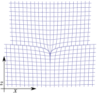
(a) $\alpha_{2}$

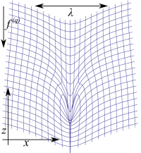
(b) $\lambda=0.6$

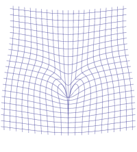
(c) $\lambda=1.2$

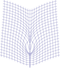
(d) Conventional, $\lambda=0.6$

Figure 1: (a) A plot of the deformation field associated with harmonic function $\alpha_{2}$ (eqn. (12)) showing promising point-force like behavior at the origin but also a discontinuity in displacement (corresponding to a dislocation) along the line $q=0$. Subfigures (b) and (c): Deformation caused by a point force of magnitude $2\mu$ in two dimensions after imposition of a large pre-strain (eqn. (19)) calculated using exact area preservation. The solutions are formed by taking superpositions of the fields $\alpha_{2}$ and $\alpha_{4}$ to cancel out their dislocations. The grids shown were square grids in the compressed base state with lattice-spacing 0.1, and the values of $\lambda$ given are the compression ratios of the pre-strain in the direction perpendicular to the direction of the force. Compression transverse to the direction of application of the force leads to substantially enhanced response. Subfigure (d): same as (b) but the traditional rather than area preserving solution.

.4 Planar Green’s functions for pre-strained half spaces

We now consider the Green’s functions for a force acting in the elastic half space $q<0$ and construct them from the full space Green’s functions via the superposition of image solutions outside of the elastic half space to satisfy the boundary conditions on the free surface. An elastic half-space has a free surface ($q=0$) which must be stress free. From eqn. (3), we see that in our case this requires

$$(\mu F_{1}\cdot F_{0}\cdot{F_{0}}^{T}-PF_{1}^{-T})\cdot(0,1)=(0,0).$$ (22)

Although this expression follows directly from eqn. (3), some readers may have been expecting it to involve the PK1 stress tensor, $\mu F_{1}\cdot F_{0}-PF_{1}^{-T})F_{0}^{-T}$, which relates reference state normals to final state forces. It does not because the unit normal in question is defined in our pre-strained elastic reference state, not the zero strain state. However, since in our case the normal is $(0,1)$ in both states (as the pre-strain does not rotate the free surface), one could in-fact use PK1 in the above expression without error. Linearizing the above in the incremental pressure $\kappa$ and the displacement potential $\alpha$ yields

$$\left(\begin{array}[]{c}-\alpha_{{qq}}+P_{0}\lambda^{2}\alpha_{{xx}}\\ 1-P_{0}\lambda^{2}-\kappa\lambda^{2}+\left(1+P_{0}\lambda^{2}\right)\alpha_{{xq}}\end{array}\right)_{q=0}=\left(\begin{array}[]{c}0\\ 0\end{array}\right).$$ (23)

Considering the case where there is no applied force, whence $\kappa=\alpha=0$, we see that $P_{0}=1/\lambda^{2}$. If $\kappa$ and $\alpha$ are given by eqn. (19) and (21) for the whole space Green’s functions corresponding to a vertical point force at $q=-d$, the left hand side of eqn. (23) is

$$\frac{f^{(q)}}{2\pi\mu\left(\lambda^{4}-1\right)}\left(\begin{array}[]{c}\frac{2x\lambda^{2}}{d^{2}+x^{2}}-\frac{x\left(1+\lambda^{4}\right)}{x^{2}+d^{2}\lambda^{4}}\\ \frac{d\lambda^{2}\left(1+\lambda^{4}\right)}{d^{2}+x^{2}}-\frac{2d\lambda^{4}}{x^{2}+d^{2}\lambda^{4}}\end{array}\right).$$ (24)

Since this is neither an even nor an odd function of $d$ we cannot use mirror image forces to satisfy the free boundary condition. However, a linear combination of four image solutions corresponding $\alpha_{2}(x,q-d),\alpha_{2}(x,q-d\lambda^{2})$ (eqn. 12 and 15) and $\alpha_{4}(x,q-d),\alpha_{4}(x,q-d/\lambda^{2})$ (eqn. (14) and (16)) gives four parameters with which to cancel out the four terms in eqn. (24). We may then write the vertical point force Green’s function for a half space as

$$\alpha^{(q)}_{hs}(x,q) =\alpha^{(q)}(x,q+d)+a_{1}\alpha_{2}(x,q-d)+a_{2}\alpha_{4}(x,q-d)+a_{3}\alpha_{2}(x,q-d\lambda^{2})+a_{4}\alpha_{4}(x,q-d/\lambda^{2}),$$

$$\kappa^{(q)}_{hs}(x,q) =\kappa^{(q)}(x,q+d)+a_{1}\kappa_{2}(x,q-d)+a_{2}\kappa_{4}(x,q-d)+a_{3}\kappa_{2}(x,q-d\lambda^{2})+a_{4}\kappa_{4}(x,q-d/\lambda^{2}),$$ (25)

and make the boundary stress-free by setting

$$a_{1}=-\frac{f^{(q)}\lambda^{2}\left(1+3\lambda^{2}-\lambda^{4}+\lambda^{6}\right)}{2\pi\mu\left(-1+\lambda^{2}\right)^{2}\left(-1+3\lambda^{2}+\lambda^{4}+\lambda^{6}\right)}\mathrm{,\ }a_{3} =\frac{2f^{(q)}\lambda^{2}\left(1+\lambda^{4}\right)}{\pi\mu\left(-1+\lambda^{2}\right)^{2}\left(1+\lambda^{2}\right)\left(-1+3\lambda^{2}+\lambda^{4}+\lambda^{6}\right)}$$

$$a_{2}=a_{1}/\lambda^{2}\mathrm{,\ \ \ \ \ \ \ \ \ \ \ \ \ \ \ \ \ \ \ \ \ \ \ \ \ \ \ \ \ \ \ \ \ \ \ \ \ \ \ \ \ \ \ \ \ \ }a_{4} =a_{3}.$$ (26)

Although these image charges are associated with line dislocations, they are along lines of constant $q$ and lie completely outside the elastic domain, so they are not physically important.

We calculate the half space Green’s function for a horizontal force in exactly the same way, now using a trial function of the form

$$\alpha^{(x)}_{hs}(x,q) =\alpha^{(x)}(x,q+d)+b_{1}\alpha_{1}(x,q-d)+b_{2}\alpha_{3}(x,q-d)+b_{3}\alpha_{1}(x,q-d\lambda^{2})+b_{4}\alpha_{3}(x,q-d/\lambda^{2})$$

$$\kappa^{(x)}_{hs}(x,q) =\kappa^{(x)}(x,q+d)+b_{1}\kappa_{1}(x,q-d)+b_{2}\kappa_{3}(x,q-d)+b_{3}\kappa_{1}(x,q-d\lambda^{2})+b_{4}\kappa_{3}(x,q-d/\lambda^{2}).$$ (27)

where the stress-free boundary condition, eqn. (23), is satisfied by the following choices of the constants:

$$b_{1}=\frac{f^{(x)}\lambda^{2}\left(1+3\lambda^{2}-\lambda^{4}+\lambda^{6}\right)}{2\pi\mu\left(-1+\lambda^{2}\right)^{2}\left(-1+3\lambda^{2}+\lambda^{4}+\lambda^{6}\right)}\mathrm{,\ }b_{3} =-\frac{2f^{(x)}\lambda^{4}\left(1+\lambda^{4}\right)}{\pi\mu\left(-1+\lambda^{2}\right)^{2}\left(1+\lambda^{2}\right)\left(-1+3\lambda^{2}+\lambda^{4}+\lambda^{6}\right)}$$

$$b_{2}=b_{1}\mathrm{,\ \ \ \ \ \ \ \ \ \ \ \ \ \ \ \ \ \ \ \ \ \ \ \ \ \ \ \ \ \ \ \ \ \ \ \ \ \ \ \ \ \ \ \ \ \ \ \ }b_{4} =b_{3}/\lambda^{2}.$$ (28)

In this case the line-dislocations associated with the image charges are all along the line $x=0$ and do penetrate the elastic half-space, so to restore the continuity of displacement in the half-space we must add a step function in displacement, by adding $\frac{f^{(x)}\lambda^{2}\left(\lambda^{2}-1\right)x(2\theta(xd)-1)}{2\mu(\lambda^{6}+\lambda^{4}+3\lambda^{2}-1)}$ to $\alpha(x,q)$ given by eqn. (27).

.5 Green’s functions for unstrained half space

Taking the isotropic limit ($\lambda\to 1$) of eqn. (25) gives the isotropic point force Green’s function as

$$\alpha(x,q) =-\frac{f^{(q)}}{8\pi\mu}\left(\frac{4dq}{(d-q)^{2}+x^{2}}+\log\left(\left((d-q)^{2}+x^{2}\right)\left((d+q)^{2}+x^{2}\right)\right)\right)$$ (29)

$$\kappa(x,q) =-\frac{f^{(q)}\left((d-q)^{2}(d+q)\left(d^{2}+2dq-q^{2}\right)-2q\left(2d^{2}-dq+q^{2}\right)x^{2}-(d+q)x^{4}\right)}{\pi\mu\left((d-q)^{2}+x^{2}\right)^{2}\left((d+q)^{2}+x^{2}\right)}.$$ (30)

for a vertical force at $(0,-d)$ in a half space, while, for a horizontal force we use of eqn. (27) to get

$$\alpha(x,q) =\frac{f^{(x)}}{8\pi\mu}\left(\frac{4\left(d^{3}-2dq^{2}+x^{2}(d+q)+q^{3}\right)}{(d-q)^{2}+x^{2}}+(d+q)\log\left(\left((d-q)^{2}+x^{2}\right)\left((d+q)^{2}+x^{2}\right)\right)\right)$$ (31)

$$\kappa(x,q) =\frac{f^{(x)}x\left(-d^{4}-4d^{3}q+4d^{2}q^{2}+\left(q^{2}+x^{2}\right)^{2}\right)}{\pi\mu\left((d-q)^{2}+x^{2}\right)^{2}\left((d+q)^{2}+x^{2}\right)}.$$ (32)

Once again, this matches the conventional Green’s functions for a point force in an elastic half-space (Melan, 1932) to linear order. In fig. 2 we compare this solution to the conventional linear elastic solution and see that while both solutions have divergent displacement and self-intersection in the neighborhood of the force, the conventional solution produces poor area conservation over a wide area, leading to substantially different forms for the free surfaces.

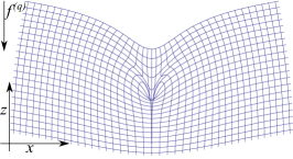
(a) Vertical area preserving solution (eqn. (29))

(b) Vertical traditional (Melan) solution

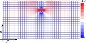
(c) Volume changes in traditional vertical solution.

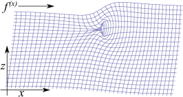
(d) Horizontal area preserving solution (eqn. (31))

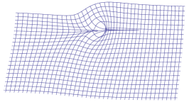
(e) Horizontal traditional (Melan) solution

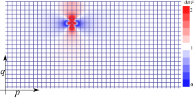
(f) Volume changes in traditional horizontal solution.

Figure 2: Deformation of a square grid with spacing 0.1 caused by a point force of strength $2\mu$ applied beneath the surface of an incompressible isotropic half-space at a location $(0,-1/2)$. Figures (a) and (d) are the exactly area preserving responses to forces applied perpendicular and parallel to the surface given by eqns. (29) and (31), while (b) and (e) are the responses given by the classical linear elastic (Melan) solutions showing severe area distortion near the point of application of the force. Figures (c) and (f) show the reference state for the two cases colored by the volume change caused by the corresponding Melan solutions.

.6 Planar higher order and surface Green’s functions

It is straightforward to combine the above Green’s functions to construct dipole and quadruple Green’s functions with and without moments. For example the Green’s function for a horizontal dipole in an uncompressed full two dimensional space is simply

$$\alpha(x,q) =\lim_{a\to 0}\left(\frac{f^{(x)}q\log\left(q^{2}+(x+a)^{2}\right)}{8\pi\mu}-\frac{f^{(x)}q\log\left(q^{2}+(x-a)^{2}\right)}{8\pi\mu}\right)=\frac{f^{(x)}qxa}{2\pi\left(q^{2}+x^{2}\right)\mu}$$ (33)

$$\kappa(x,q) =\lim_{a\to 0}\left(\frac{f^{(x)}(a+x)}{2\pi\mu\left(q^{2}+(a+x)^{2}\right)}-\frac{f^{(x)}(-a+x)}{2\pi\mu\left(q^{2}+(-a+x)^{2}\right)}\right)=\frac{f^{(x)}\left(q^{2}-x^{2}\right)a}{\pi\mu\left(q^{2}+x^{2}\right)^{2}}.$$ (34)

We can also look at the limit $d\to 0$ to find the Green’ s functions for a point force acting on the surface of a half space. Since taking these limits is straightforward, we do not explicitly calculate any examples here but some higher order and surface solutions are shown in tables 1 and 2.

Description	$\alpha(x,q)$	$\kappa(x,q)$
Isotropic full-space horizontal dipole	$\frac{qx}{2\pi\left(q^{2}+x^{2}\right)}$	$\frac{(q-x)(q+x)}{\pi\left(q^{2}+x^{2}\right)^{2}}$
Pre-strained full- Space horizontal dipole	$\frac{\lambda^{2}\left(\tan^{-1}\left(\frac{q\lambda^{2}}{x}\right)-\tan^{-1}\left(\frac{q}{x}\right)\right)}{\pi\left(\lambda^{4}-1\right)}$	$\frac{(q-x)(q+x)}{\pi\left(q^{2}+x^{2}\right)^{2}}$
Isotropic full-space vertical dipole	$\frac{qx}{2\pi\left(q^{2}+x^{2}\right)}$	$\frac{(q-x)(q+x)}{\pi\left(q^{2}+x^{2}\right)^{2}}$
Pre-strained full-space vertical dipole	$\frac{\lambda^{2}\left(\tan^{-1}\left(\frac{x}{q}\right)-\tan^{-1}\left(\frac{x}{q\lambda^{2}}\right)\right)}{\pi\left(\lambda^{4}-1\right)}$	$\frac{(q-x)(q+x)}{\pi\left(q^{2}+x^{2}\right)^{2}}$
Pre-strained full-space horizontal quadrupole	$\frac{q\lambda^{2}(-x+q\lambda)(x+q\lambda)}{2\pi\left(q^{2}+x^{2}\right)\left(1+\lambda^{2}\right)\left(x^{2}+q^{2}\lambda^{4}\right)}$	$\frac{x\left(-3q^{2}+x^{2}\right)}{\pi\left(q^{2}+x^{2}\right)^{3}}$
Pre-strained full-space vertical quadrupole	$\frac{x\lambda^{2}(x-q\lambda)(x+q\lambda)}{2\pi\left(q^{2}+x^{2}\right)\left(1+\lambda^{2}\right)\left(x^{2}+q^{2}\lambda^{4}\right)}$	$-\frac{q\left(q^{2}-3x^{2}\right)}{\pi\left(q^{2}+x^{2}\right)^{3}}$

Table 1: Full space higher order Green’s functions.

Description	$\alpha(x,q)$	$\kappa(x,q)$
Isotropic half-space vertical force	$\frac{-f^{(q)}x\log\left(q^{2}+x^{2}\right)}{4\pi\mu}$	$\frac{f^{(q)}q}{\pi\mu\left(q^{2}+x^{2}\right)}$
Isotropic half-space horizontal force	$\frac{f^{(x)}q\left(\log\left(q^{2}+x^{2}\right)+2\right)}{4\pi\mu}$	$\frac{f^{(x)}x}{\pi\mu\left(q^{2}+x^{2}\right)}$
Pre-strained half-space vertical force	$\frac{-f^{(q)}\lambda^{2}}{2\mu\pi\left(\lambda^{8}+2\lambda^{4}-4\lambda^{2}+1\right)}\left(2q\left(\lambda^{4}+1\right)\tan^{-1}\left(\frac{x}{q}\right)-4q\lambda^{2}\tan^{-1}\left(\frac{x}{q\lambda^{2}}\right)\right.$ $\left.+x\left(\lambda^{4}+1\right)\log\left(q^{2}+x^{2}\right)-2x\log\left(q^{2}\lambda^{4}+x^{2}\right)\right)$	$\frac{f^{(q)}q\left(1+\lambda^{2}\right)\left(1+\lambda^{4}\right)}{\pi\mu\left(q^{2}+x^{2}\right)\left(-1+3\lambda^{2}+\lambda^{4}+\lambda^{6}\right)}$
Pre-strained half-space horizontal force	$\frac{-f^{(x)}\lambda^{2}}{2\mu\pi\left(\lambda^{8}+2\lambda^{4}-4\lambda^{2}+1\right)}\left(4x\lambda^{2}\tan^{-1}\left(\frac{q}{x}\right)-2x\left(\lambda^{4}+1\right)\tan^{-1}\left(\frac{q\lambda^{2}}{x}\right)\right.$ $\left.-q\lambda^{2}\left(\left(\lambda^{4}+1\right)\log\left(q^{2}\lambda^{4}+x^{2}\right)-2\log\left(q^{2}+x^{2}\right)\right)\right.$ $\left.+x\pi\left(-1+\lambda^{2}\right)^{2}(1-2\theta(x))\right)$	$\frac{2f^{(x)}x\lambda^{2}\left(1+\lambda^{2}\right)}{\pi\mu\left(q^{2}+x^{2}\right)\left(-1+3\lambda^{2}+\lambda^{4}+\lambda^{6}\right)}$

Table 2: Half space surface force Green’s functions

I Exact volume conservation for three-dimensional axisymmetric deformations

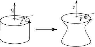
Figure 3: A three dimensional axisymmetric elastic body (left) labeled by the coordinates $(\rho,\theta,q)$ is deformed into the target state (right) labeled by the coordinates $(r,\phi,z)$.

We now turn to 3d axisymmetric deformations of incompressible materials. We consider a neo-Hookean elastic body labeled by the polar-coordinate system $(\rho,\theta,q)$ in the reference state that is deformed into a target or current state parameterized by $(r,\phi,z)$, depicted in fig. 3. We usually describe an axisymmetric deformation with functions $r(\rho,q)$ and $z(\rho,q)$, with axisymmetry requiring that $\phi=\theta$ for each point in the elastic body. Within this description, in a polar coordinate system, the deformation gradient tensor is

$$F_{1}(\rho,q)=\left(\begin{array}[]{ccc}\frac{\partial r}{\partial\rho}\big{|}_{q}&0&\frac{\partial r}{\partial q}\big{|}_{\rho}\\ \ 0&r/\rho&0\\ \frac{\partial z}{\partial\rho}\big{|}_{q}&0&\frac{\partial z}{\partial q}\big{|}_{\rho}\end{array}\right).$$ (35)

Once again the constraint of volume conservation requires that ${\rm det}F_{1}=1$. As in the 2-D case, we include the possibility that, in the $\rho-q$ elastic reference state the material has already undergone an axisymmetric and volume preserving pre-strain $F_{0}=\mathrm{diag}(\lambda,\lambda,1/\lambda^{2})$, so that the total deformation from the unstrained state is $F_{1}\cdot F_{0}$. Again, as in the 2-D case, the equations of equilibrium are then

$$\nabla\cdot(\mu F_{1}\cdot F_{0}\cdot{F_{0}}^{T}-PF_{1}^{-T})=-\mathbf{f}\hskip 30.00005pt{\rm Det}\!\left(F_{1}\right)=1,$$ (36)

with the divergence being taken in the $(\rho,\theta,q)$ reference state. Inspired by the Gaussian incompressible mapping in the two dimensional case, we choose to instead represent the deformation $F_{1}$ via the functions $\rho(r,q)$ and $z(r,q)$ that reside partly in the reference and partly in the current configurations, so that $F_{1}$ becomes

$$F_{1}(r,q)=\left(\begin{array}[]{ccc}\left(\frac{\partial\rho}{\partial r}\big{|}_{q}\right)^{-1}&0&-\frac{\partial\rho}{\partial q}\big{|}_{r}\left(\frac{\partial\rho}{\partial r}\big{|}_{q}\right)^{-1}\\ \ 0&r/\rho&0\\ \frac{\partial z}{\partial r}\big{|}_{q}\left(\frac{\partial\rho}{\partial r}\big{|}_{q}\right)^{-1}&0&\frac{\partial z}{\partial q}\big{|}_{r}-\frac{\partial\rho}{\partial q}\big{|}_{r}\frac{\partial z}{\partial r}\big{|}_{q}\left(\frac{\partial\rho}{\partial r}\big{|}_{q}\right)^{-1}\end{array}\right).$$ (37)

Assuming all quantities are functions of $r$ and $q$, so that $\rho_{r}=\frac{\partial\rho}{\partial r}\big{|}_{q}$, we can calculate

$$\det{F_{1}}=\frac{rz_{q}}{\rho\rho_{r}}.$$ (38)

To enforce perfect volume conservation, we introduce the scalar field $\chi(r,q)$ defined by the relations

$$z(r,q)=\frac{\chi_{r}}{r}\mathrm{\ \ \ \ \ and\ \ \ \ \ \ }\rho(r,q)=\sqrt{2\chi_{q}},$$ (39)

so that $\det{F}=\left.\left(r\frac{1}{r}\chi_{rq}\right)\middle/\left(\rho(2\chi_{q})^{-1/2}\chi_{rq}\right)\right.=1.$ In terms of this new field, the deformation gradient is

$$F_{1}(r,q)=\left(\begin{array}[]{ccc}\frac{\sqrt{2\chi_{q}}}{\chi_{{rq}}}&0&-\frac{\chi_{{qq}}}{\chi_{{rq}}}\\ 0&\frac{r}{2\sqrt{\chi_{q}}}&0\\ \frac{\sqrt{2\chi_{q}}\left(-\chi_{r}+r\chi_{{rr}}\right)}{r^{2}\chi_{{rq}}}&0&\frac{r\chi_{{rq}}^{2}+\chi_{{qq}}\left(\chi_{r}-r\chi_{{rr}}\right)}{r^{2}\chi_{{rq}}}\end{array}\right).$$ (40)

I.1 Incremental axisymmetric three dimensional elasticity

Before any additional displacement ($F_{1}=I$) we have $\chi={\textstyle\frac{1}{2}}r^{2}q$ and $P=\mu P_{0}$, where $\mu P_{0}$ may be a large pressure associated with the pre-strain. To linearize about this reference state, we write

$$\chi(r,q)={\textstyle\frac{1}{2}}r^{2}q+\beta(r,q)\mathrm{,\ \ \ \ and\ \ \ \ }P(r,q)=\mu P_{0}+\mu\kappa(r,q),$$ (41)

where $\beta,\mathrm{\ }\kappa<<1$. Expanding $F$ and $F^{-T}$ to linear order in $\beta$ give

$$F=\left(\begin{array}[]{ccc}1+\frac{\beta_{q}-r\beta_{qq}}{r^{2}}&0&-\frac{\beta_{qq}}{r}\\ 0&1-\frac{\beta_{q}}{r^{2}}&0\\ \frac{r\beta_{rr}-\beta_{r}}{r^{2}}&0&1+\frac{\beta_{qq}}{r}\\ \end{array}\right)\hskip 30.00005ptF^{-T}=\left(\begin{array}[]{ccc}1-\frac{\beta_{q}-r\beta_{qq}}{r^{2}}&0&\frac{\beta_{r}-r\beta_{rr}}{r^{2}}\\ 0&1+\frac{\beta_{q}}{r^{2}}&0\\ \frac{\beta_{qq}}{r}&0&1-\frac{\beta_{qq}}{r}\\ \end{array}\right).$$ (48)

As claimed in our letter, these forms are algebriacally identical to those that would be derived by introducing a traditional Stokes stream line function $\beta(\rho,q)$ such that $r=\rho-(1/\rho)\beta_{q}$ and $z=q+(1/r)\beta_{\rho}$, with the identification $\rho\to r$. We then find the linearized equations of equilibrium by substituting these results into eqn. (36), and expanding to first order. To conduct the expansion we must recall the form for the divergence of a tensor in cylindrical polars (see, for example Bower (2011) Appendix D) and make use of the first order partial derivative identities $\frac{\partial}{\partial\rho}\big{|}_{q}=\frac{\partial}{\partial r}\big{|}_{q}$ and $\frac{\partial}{\partial q}\big{|}_{\rho}=\frac{\partial}{\partial q}\big{|}_{r}$, to get

$$\frac{\mu}{\lambda^{4}r^{2}}\left(\begin{array}[]{c}-r^{2}\lambda^{4}\kappa_{r}-r\beta_{{qqq}}+\lambda^{6}\left(\beta_{{rq}}-r\beta_{{rrq}}\right)\\ -r^{2}\lambda^{4}\kappa_{q}+r\beta_{{rqq}}+\lambda^{6}\left(r\beta_{{rrr}}-\beta_{{rr}}+\beta_{r}/r\right)\end{array}\right)=-\mathbf{f}.$$ (49)

In a region with no external force ($\mathbf{f}=0$) we can once again eliminate $\kappa$ to get the axsysmetric version of the 2D eqn. (6),

$$\left(\lambda^{6}r\frac{\partial}{\partial r}\left(\frac{1}{r}\frac{\partial}{\partial r}\right)+\frac{\partial^{2}}{\partial q^{2}}\right)\left(r\frac{\partial}{\partial r}\left(\frac{1}{r}\frac{\partial}{\partial r}\right)+\frac{\partial^{2}}{\partial q^{2}}\right)\beta(r,q)=0.$$ (50)

In the case where there is no pre-strain ($\lambda=1$) these two equations reduce to

$$\frac{\mu}{r^{2}}\left(\begin{array}[]{c}\beta_{{rq}}-r(r\kappa_{r}+\beta_{{qqq}}+\beta_{{rrq}})\\ -r^{2}\kappa_{q}+r(\beta_{{rqq}}+\beta_{{rrr}})-\beta_{{rr}}+\beta_{r}/r\end{array}\right)=-\mathbf{f}.$$ (51)

and an axisymmetric analog of the biharmonic equation discussed in our letter,

$$\left(r\frac{\partial}{\partial r}\left(\frac{1}{r}\frac{\partial}{\partial r}\right)+\frac{\partial^{2}}{\partial q^{2}}\right)^{2}\beta=0.$$ (52)

I.2 Axisymmetric Green’s functions for unstrained full space

In three dimensions, for a force along the axis of symmetry, we expect the displacement to vary inversely as the distance from the point of application of the force, so $\beta$ should increase proportional to the distance from the point of application, leading us to the suggestion that

$$\beta(r,q)=A\frac{r^{2}}{(q^{2}+r^{2})^{1/2}}+B\frac{q^{2}}{(q^{2}+r^{2})^{1/2}}.$$ (53)

This function satisfies the equation of equilibrium (eqn. (52)), but axisymmetry requires that $\rho(0,q)=0$, so $B=0$. Substituting $\beta$ into eqn. (51), we find that $\kappa(r,q)=2Aq\left(q^{2}+r^{2}\right)^{-3/2}$. Normalizing this function so that it is the response to a total force $f$, the Green’s functions are

$$\beta(r,q)=\frac{fr^{2}}{8\pi\mu\sqrt{q^{2}+r^{2}}}\mathrm{\ \ \ \ and\ \ \ \ }\kappa(r,q)=\frac{fq}{4\pi\mu\left(q^{2}+r^{2}\right)^{3/2}},$$ (54)

which, at linear-order, match the elementary Kelvin solution (Thomson, Lord Kelvin) in linear elasticity.

Since we are restricted to axisymmetric situations we cannot consider point-forces in other directions acting on the axis, or point forces in any direction acting away from the axis. However, we can consider both radial and axial forces acting in rings around the axis. In these cases there are no simple scaling arguments that can be used to produce the solutions. In conventional linear elasticity the Green’s function for a ring-load can be found by using the elastic reciprocal theorem (Kermanidis, 1975) or integrating the point-force solution around a ring (Hanson and Wang, 1997). Here, we find these Green’s functions by taking these traditional results, expressing them (for the incompressible case) via the traditional Stokes streamline function then identifying $\rho\to r$. For a ring load applying a force along the axis, we get

$$\beta^{(Ra)}(r,q) =\frac{f^{(a)}}{8\pi^{2}\mu}\sqrt{(a+r)^{2}+q^{2}}\left(\left(\frac{2r(a+r)}{(a+r)^{2}+q^{2}}-1\right)K\left(\frac{4ar}{q^{2}+(a+r)^{2}}\right)+E\left(\frac{4ar}{q^{2}+(a+r)^{2}}\right)\right)$$ (55)

$$\kappa^{(Ra)}(r,q) =\frac{f^{(a)}}{4\pi^{2}\mu}\frac{2qE\left(\frac{4ar}{q^{2}+(a+r)^{2}}\right)}{\left((a-r)^{2}+q^{2}\right)\sqrt{(a+r)^{2}+q^{2}}},$$ (56)

where $f^{(a)}$ is the total force in the applied in the axial direction along a ring of radius $a$ and $K(m)=\int_{0}^{\pi/2}\frac{\mathrm{d}\theta}{\sqrt{1-m\sin^{2}{\theta}}}$ and $E(m)=\int_{0}^{\pi/2}\sqrt{1-m\sin^{2}{\theta}}\mathrm{d}\theta$ are the complete elliptic integrals of the first and second kind. Similarly, if the applied force is in the radial direction along the same ring, the Green’s function are:

$$\beta^{(Rr)}(r,q) =\frac{f^{(r)}q\left(\left((a+r)^{2}+q^{2}\right)E\left(\frac{4ar}{q^{2}+(a+r)^{2}}\right)-\left(a^{2}+q^{2}+r^{2}\right)K\left(\frac{4ar}{q^{2}+(a+r)^{2}}\right)\right)}{8\pi^{2}a\mu\sqrt{(a+r)^{2}+q^{2}}}$$ (57)

$$\kappa^{(Rr)}(r,q) =\frac{f^{(r)}\left(\left(-a^{2}+q^{2}+r^{2}\right)E\left(\frac{4ar}{q^{2}+(a+r)^{2}}\right)-\left((a-r)^{2}+q^{2}\right)K\left(\frac{4ar}{q^{2}+(a+r)^{2}}\right)\right)}{4\pi^{2}a\mu\left((a-r)^{2}+q^{2}\right)\sqrt{(a+r)^{2}+q^{2}}}.$$ (58)

These two solutions are plotted in fig. 4. As before there is some self intersection near the point of application of the force caused by the divergent stress, where the solution is expected to break down.

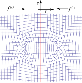
(a) Inward ring-load.

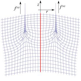
(b) Upward ring load.

Figure 4: Exactly volume preserving deformation caused by an inward radial ring load (left, eqn. (57)) and an upward radial ring load (right, eqn. (55)). The red line indicates the axis of symmetry, the grid was a square lattice with spacing $0.1$ in the reference state, the total force applied in both cases is $2\pi\mu$, and the ring is located at $r=0.55$.

I.3 Axisymmetric Green’s functions for pre-strained full space

As in the case without the pre-strain, we expect $\beta(r,q)$ to be proportional to distance from the point of application of the force. Taking inspiration from the analogous 2-D case, the simplest functions with this scaling at large distances which satisfy the equation (50) for $\beta$ are $\beta_{1}=\sqrt{r^{2}+q^{2}},$ and $\beta_{2}=\sqrt{r^{2}+\lambda^{6}q^{2}}$. Substituting these forms into eqn. (49), we see the incremental pressures associated with them are

$$\kappa_{1}(r,q)=\frac{q\left(-1+\lambda^{6}\right)}{\left(q^{2}+r^{2}\right)^{3/2}\lambda^{4}}\mathrm{\ \ \ \ and\ \ \ \ }\kappa_{2}(r,q)=0.$$ (59)

However, as in the 2-dimensional case, these are not admissible deformations because $\rho(0,q)\neq 0$. As in the 2-D case, we can take a linear combination of $\beta_{1}$ and $\beta_{2}$ that is admissible:

$$\beta^{(a)}(r,q)=\frac{f\lambda}{4\pi\mu\left(\lambda^{6}-1\right)}\left(\lambda^{3}\sqrt{q^{2}+r^{2}}-\sqrt{r^{2}+q^{2}\lambda^{6}}\right).$$ (60)

Taking the same linear combination of $\kappa_{1}$ and $\kappa_{2}$ we see the incremental pressure field is given by

$$\kappa^{(a)}(r,q)=\frac{fq}{4\pi\mu\left(q^{2}+r^{2}\right)^{3/2}}.$$ (61)

The pre factor has been chosen by integration of the stress over an infinite cylinder oriented along the axis of symmetry. The ring-load Green’s functions in the presence of a large pre-stress are not expressible in closed form, so they will not be presented here.

I.4 Green’s functions for half spaces with large pre-strains

We find the on-axis half-space Green’s function for an axially symmetric point force at $(0,-d)$ in an analogous way to the planar problem treated earlier. The bulk equations of equilibrium (eqns. (49)) are now supplemented by the condition that the free surface at $q=0$ be stress free, which, from eqn. (36), we see reads

$$(\mu F_{1}\cdot F_{0}\cdot F_{0}^{T}-PF_{1}^{-T})\cdot(0,0,1)=(0,0,0).$$ (62)

Linearizing this with respect to $\beta$ and $\kappa$ yields

$$\frac{\mu}{r^{2}\lambda^{4}}\left(\lambda^{4}P_{0}\left(r\beta_{rr}(r,0)-\beta_{r}(r,0)\right)-r\beta_{qq}(r,0),0,r\left(\left(\lambda^{4}P_{0}+1\right)\beta_{qq}(r,0)-\lambda^{4}r\kappa(r,0)\right)+r^{2}\left(1-\lambda^{4}P_{0}\right)\right)=\left(0,0,0\right).$$ (63)

Setting $\beta\to 0$ and $\kappa\to 0$, we see that $P_{0}=1/\lambda^{4}$. Inspired by the solution in the 2-D place, we then try for the 3-D half space solution the whole space Green’s function (eqns. (60) and (61)) at a depth $d$ below the free surface augmented by image forces above the half space, in the form

$$\beta(x,q) =\beta^{(a)}(r,q+d)+a_{1}\beta_{1}(r,q-d)+a_{2}\beta_{2}(r,q-d)+a_{3}\beta_{1}(r,q-d\lambda^{3})+a_{4}\beta_{2}(r,q-d/\lambda^{3})$$

$$\kappa(x,q) =\kappa^{(a)}(r,q+d)+a_{1}\kappa_{1}(r,q-d)+a_{2}\kappa_{2}(r,q-d)+a_{3}\kappa_{1}(r,q-d\lambda^{3})+a_{4}\kappa_{2}(r,q-d/\lambda^{3}),$$ (64)

analogous to eqn. (25). We can then satisfy the boundary condition with the choices:

$$a_{1}=\frac{f\lambda^{4}\left(1+3\lambda^{3}-\lambda^{6}+\lambda^{9}\right)}{4\pi\left(-1+\lambda^{3}\right)^{2}\left(-1+3\lambda^{3}+\lambda^{6}+\lambda^{9}\right)\mu}\mathrm{,\ }a_{3} =\frac{-f\lambda^{4}\left(1+\lambda^{6}\right)}{\pi\left(-1+\lambda^{3}\right)^{2}\left(1+\lambda^{3}\right)\left(-1+3\lambda^{3}+\lambda^{6}+\lambda^{9}\right)\mu}$$

$$a_{2}=a_{1}/\lambda^{3}\mathrm{,\ \ \ \ \ \ \ \ \ \ \ \ \ \ \ \ \ \ \ \ \ \ \ \ \ \ \ \ \ \ \ \ \ \ \ \ \ \ \ \ \ \ \ \ \ }a_{4} =a_{3}.$$ (65)

As in the two dimensional case, although these fields satisfy the equations of mechanical equilibrium (eqn. (49)) and the boundary condition (eqn. (62)), they are not admissible because they do not have continuous displacements since $\rho(0,q)\neq 0$. However, we can fix this by adding $\frac{qf\lambda^{4}\left(-1+\lambda^{3}\right)}{2\pi\left(-1+3\lambda^{3}+\lambda^{6}+\lambda^{9}\right)\mu}$ to $\beta$ given in eqn. (64), which does not give rise to any (first order) stress or strain but removes the discontinuity at the origin. No modification to $\kappa$ is required.

I.5 Axisymmetric Green’s functions for unstrained half space

Taking the isotropic limit ($\lambda\to 1$) of eqn. (64) gives the point force half space Green’s function as

$$\beta(r,q)=\frac{fr^{2}}{8\pi\mu}\left(\frac{1}{\sqrt{(d-q)^{2}+r^{2}}}+\frac{1}{\sqrt{(d+q)^{2}+r^{2}}}-\frac{2dq}{\left((d-q)^{2}+r^{2}\right)^{3/2}}\right)$$ (66)

$$\kappa(r,q)=\frac{f}{4\pi\mu}\left(\frac{d+q}{\left((d+q)^{2}+r^{2}\right)^{3/2}}-\frac{(d-q)^{2}(5d-q)-(d+q)r^{2}}{\left((d-q)^{2}+r^{2}\right)^{5/2}}\right),$$ (67)

which matches Mindlin’s solution (Mindlin, 1936) to linear order. Taking $d\to 0$ gives the surface Green’s functions, corresponding to those found by Boussinesq (Boussinesq, 1885) and Cerruti (Cerruti, 1893).

Isotropic half-space ring-load Green’s functions are known in conventional linear elasticity (Hanson and Wang, 1997). Ours will be the same combination of image forces. For an axial ring loading this is:

$$\beta(r,q) =\beta^{(Ra)}(r,q+d)+\beta^{(Ra)}(r,q-d)+\frac{2dq}{q-d}\beta^{(Ra)}_{q}(r,q-d)$$ (68)

$$\kappa(r,q) =\kappa^{(Ra)}(r,q+d)+\kappa^{(Ra)}(r,q-d)+2d\kappa^{(Ra)}_{q}(r,q-d),$$ (69)

while for a radial ring loading we have:

$$\beta(r,q) =\beta^{(Rr)}(r,q+d)+\beta^{(Rr)}(r,q-d)+\frac{2d(2q-d)}{(d-q)^{2}}\beta^{(Rr)}(r,q-d)+\frac{2dq}{d-q}\beta^{(Rr)}_{q}(r,q-d)$$

$$\kappa(r,q) =\kappa^{(Rr)}(r,q+d)+\kappa^{(Rr)}(r,q-d)-2d\kappa^{(Rr)}_{q}(r,q-d),$$ (70)

where $\beta^{(Rr)}$ etc. are the full space ring Green’s functions given in eqns. (55-58).

As in the full-space case, it is simple but algebraically very laborious to show that these fields satisfy the bulk and boundary equations (but see Supplementary Mathematica notebooks). These solutions are plotted in fig. 5. We find that the strains are higher than those in the full space case (fig. 4).

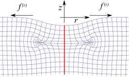
(a) Half-space outward ring-load.

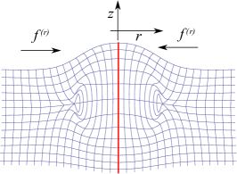
(b) Half-space inward ring-load.

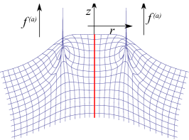
(c) Half-space upward ring load.

Figure 5: Deformation caused by outward and inward radial ring loads (subfigures a and b, eqn. (70) and an upward ring load (right, eqn. (68)) in an axisymmetric half-space. The red line indicates the axis of symmetry, the grid was a square lattice with spacing $0.1$ in the reference state and the ring is located at $r=0.55$. The force applied was $2\pi\mu$ for the inward and upward loadings and $\pi\mu$ for the outward loading.

II Surface instability deduced from half space Green’s functions

As first shown by Biot (Biot, 1965) the surface of compressed elastic half spaces become unstable to the formation of creases at a critical large compression, although recent results have shown that before this instability is reached, there is a sub-critical instability with no nucleation threshold (Hohlfeld and Mahadevan, 2011, 2012). While the nonlinear instability can not be deduced from a linear calculation as here, it is worth mentioning that the original Biot instability manifests itself in the half space Green’s functions for pre-strained solids. This is most clearly seen in the dependence of the functions via the pre-strain $\lambda$ in the image-charge potentials. At the point of instability the dependence lead to a diverging response and a reversal in the sign of the displacement caused by a force. In the two-dimensional case, the response of the half-space diverges when the denominator in eqn. (26) vanishes, which is when $-1+3\lambda^{2}+\lambda^{4}+\lambda^{6}=0$, so that the instability occurs when

$$\lambda^{*}=\frac{1}{3}\left(-1-2\left(17+3\sqrt{33}\right)^{-1/3}+\left(17+3\sqrt{33}\right)^{1/3}\right)\approx 0.543689...$$ (71)

The denominator also vanishes when $\lambda=1$, but in this case the images associated with $a_{1}$ and $a_{3}$ collapse onto the same point and cancel out, so there is no divergent response. Similarly, in the three-dimensional axisymmetric case, the onset of instability occurs when the denominator in eqn. (65) vanishes, which occurs when $-1+3\lambda^{3}+\lambda^{6}+\lambda^{9}=0$, giving

$$\lambda^{*}=\left(\frac{1}{3}\left(-1-4\times 2^{2/3}\left(13+3\sqrt{33}\right)^{-1/3}+\left(26+6\sqrt{33}\right)^{1/3}\right)\right)^{1/3}\approx 0.666142...$$ (72)

These thresholds agree with those originally found by Biot (Biot, 1965). This is expected in the planar case, but is perhaps surprising in the axisymmetric case where Biot included an axisymmetric pre-strain, but only accounted for two dimensional plane-strain perturbations. A recent numerical study of the axisymmetric Biot problem confirms this result (Tallinen et al., 2013). Our results are for the simplest possible non-linear elastic constitutive relation (neo-Hookean) but the surface instability is found in a very wide class of materials (Brun et al., 2003).

References

- Biot (1965) M. Biot, Mechanics of incremental deformations: theory of elasticity and viscoelasticity of initially stressed solids and fluids, including thermodynamic foundations and applications to finite strain (Wiley New York:, 1965).
- Hohlfeld and Mahadevan (2011) E. Hohlfeld and L. Mahadevan, Physical review letters 106, 105702 (2011).
- Biggins et al. (2008) J. Biggins, E. Terentjev, and M. Warner, Physical Review E 78, 041704 (2008).
- Ben Amar and Ciarletta (2010) M. Ben Amar and P. Ciarletta, J Mech Phys Solids 58, 935 (2010).
- Ting (1996) T. Ting, Anisotropic elasticity: theory and applications (Oxford University Press, USA, 1996).
- Bigoni and Capuani (2002) D. Bigoni and D. Capuani, Journal of the Mechanics and Physics of Solids 50, 471 (2002).
- Melan (1932) E. Melan, Z. Angew. Math. Mech 12, 343 (1932).
- Bower (2011) A. F. Bower, Applied mechanics of solids (CRC press, http://solidmechanics.org, 2011).
- Thomson (Lord Kelvin) W. Thomson (Lord Kelvin), Mathematical and Physical Papers (London) 1, 97 (1848).
- Kermanidis (1975) T. Kermanidis, International Journal of Solids and Structures 11, 493 (1975).
- Hanson and Wang (1997) M. Hanson and Y. Wang, International journal of solids and structures 34, 1379 (1997).
- Mindlin (1936) R. Mindlin, Physics 7, 195 (1936).
- Boussinesq (1885) J. Boussinesq, Application des potentiels à l’étude de l’équilibre et du mouvement des solides élastiques: principalement au calcul des déformations et des pressions que produisent, dans ces solides, des efforts quelconques exercés sur une petite partie de leur surface ou de leur intérieur: mémoire suivi de notes étendues sur divers points de physique, mathematique et d’analyse (Gauthier-Villars, 1885).
- Cerruti (1893) V. Cerruti, Il Nuovo Cimento (1877-1894) 34, 115 (1893).
- Hohlfeld and Mahadevan (2012) E. Hohlfeld and L. Mahadevan, Phys. Rev. Lett. 109, 025701 (2012).
- Tallinen et al. (2013) T. Tallinen, J. S. Biggins, and L. Mahadevan, Phys. Rev. Lett. 110, 024302 (2013).
- Brun et al. (2003) M. Brun, D. Capuani, and D. Bigoni, Computer methods in applied mechanics and engineering 192, 2461 (2003).