Periodic solutions to a mean-field model for electrocortical activity

Abstract

We consider a continuum model of electrical signals in the human cortex, which takes the form of a system of semilinear, hyperbolic partial differential equations for the inhibitory and excitatory membrane potentials and the synaptic inputs. The coupling of these components is represented by sigmoidal and quadratic nonlinearities. We consider these equations on a square domain with periodic boundary conditions, in the vicinity of the primary transition from a stable equilibrium to time-periodic motion through an equivariant Hopf bifurcation. We compute part of a family of standing wave solutions, emanating from this point.

1 Introduction

A salient, if ill-understood, feature of the human cortex is that it produces electrical fields that can be coherent on a length scale of millimetres to centimetres and a time scale of milliseconds to seconds. The biophysical origin of such fields can be explained accurately in terms of the physiology of the neurons, densely packed in the cortical layers Nunez2006 . When hundreds of thousands of neurons, spread out over a few square centimetres of cortical tissue, fire synchronously, they can produce an electrical field strong enough to measure on top of the scalp. This measurement is called the electroencephalograph (EEG), and has been used over the past century to uncover coherence in electrocortical activity. It is non-invasive and cheap compared to more recently introduced imaging techniques, such as functional Magnetic Resonance Imaging (fMRI). Although it does not have great spatial resolution, due to the spreading of signals in the scalp, its temporal resolution is high, and it has been used in countless experiments probing the processing of sensory stimuli, the generation of pathological states such as seizures and aspects of cognition.

From this body of experimental work, we have learned a lot about the phenomenology of electrical activity in the cortex. For instance, it is known that fluctuations at different frequencies play different roles in the processing of stimuli. Activity in the alpha band (8–13Hz) appears to indicate “readiness”, a state the cortex can easily move to and from during processing Liley2009 , while gamma-band oscillations (30-100Hz) are thought to facilitate the integration of networks of neurons into coherent activity (e.g. rolls2012 and references therein). Experimental work has also enabled the use of the EEG for diagnostic purposes, for instance when deciding on treatment for epilepsy or to assess the level of consciousness of patients under anaesthesia.

In contrast, questions pertaining to the organisation and dynamics of coherent electrical activity, as well as to its role in high-level brain function, are much harder to answer. Fundamental questions, such as whether alpha-band activity is generated by the cortex itself, or is a result of interaction with deeper brain structures like the thalamus, are, as yet, unanswered. To address such questions, phenomenology alone does not suffice; we need to integrate observations with predictive models.

The two most common approaches to modelling electrocortical activity are based on the simultaneous simulation of many individual, coupled neurons and on coarse-grained simulations of ensembles of neurons. In the former approach, a large, densely connected network of elementary neuronal units is time-stepped, and the macroscopic electrical potential can be reconstructed by summing over the individual outputs. Using state-of-the-art computing facilities, as many as one million units, tied together by half a billion connections, have been simulated and tuned to mimic output measured in vitro in small mammals izhi2008 . In the latter approach, mean properties of ensembles of neurons are modeled directly. The dependent variables can then be thought of as locally averaged over an area of about one square millimetre. This is often labeled the mean field approach. Under simplifying assumptions on the stochastic nature of individual neuron dynamics and on the density of their connections, mean field models can be derived from “many neuron models” as a kind of thermodynamic limit deco2008 .

Mean-field models, in turn, come in different flavours. One important distinction is that between convolution-based models and conductance-based models pinotsis2013 . In the former, the time derivatives of the mean fields are given directly by convolutions of these fields with kernels that specify the connectivity. A classical example is the Wilson-Cowan model wilson1973 , in which the fields represent the fractions of excitatory and inhibitory neurons that are firing. In the latter, the fields typically represent the mean excitatory and inhibitory membrane potential and the conductances associated with the synaptic coupling between them. Within the class of conductance-based models, there are several different types of models, distinguished by the way the input into a local cluster of neurons is computed from the global fields. This relation is most naturally expressed in terms of an integral over inputs, originating anywhere on the cortical surface, with a kernel that specifies the connection strength and delay time as a function of the distance to the source. This formulation results in a system of nonlinear integro-differential equations with distributed delays. Both the theoretical and the numerical treatment of such models is very challenging. Although much progress has been made in the analysis of simplified models, for instance with only a single neuronal population or only a single spatial dimension (see, e.g. meijer2014 ; bressloff2012 ), a direct analysis of full-fledged models of this kind is not yet feasible.

A great simplification is achieved by approximating the delay integro-differential equations by damped wave equations, a step explained in detail by Liley et al. liley2002 . The result is a system of nonlinear Partial Differential Equations (PDEs), which can be investigated in terms of the theory of continuous dynamical systems, not dissimilar to, for instance, the Navier-Stokes equations for fluid motion. This analysis is still quite challenging for a number of reasons, including

• the strong nonlinearities, in particular the sigmoidal functions that relate the change in conductance to pre-synaptic inputs;

• the large number of parameters, upon which the dynamics can depend very sensitively;

• the difficulty in determining physiologically acceptable boundary conditions and

• the presence of continuous and discrete symmetries, depending on the choice of boundary conditions.

For this reason, a lot of work on PDE-based mean field models focused on parameter regimes where a stable equilibrium state exists (e.g. bojak2005 ; pinotsis2013 ). In this work, the response of the mean-field models to noisy external input was investigated, and it was found that the models can reproduce realistic temporal spectra for the membrane potentials, which can be compared to EEG spectra.

In the current work, we attempt to study the dynamical repertoire of a PDE-based mean field model beyond the primary instability of the equilibrium state. We focus on Liley’s model, which describes both inhibitory and excitatory populations and their short range and long range connections liley2002 . In total, there are fourteen fields that satisfy either local equations or hyperbolic, semilinear PDEs. In earlier work, we reported on the software package MFM for the simulation of this model green2013 . Here, we present the computation of a spatially inhomogeneous, time-periodic solution, which takes the form of a standing wave, or a standing square in the language of equivariant bifurcation theory. As far as we are aware, this is the first such computation in a PDE-based mean field model with both excitatory and inhibitory populations and two spatial dimensions. We hypothesize that, when continued in an external input parameter, this periodic orbit will exhibit the formation of “hot spots” of gamma-band activity seen in the highly nonlinear regime of this model bojak2007 .

2 Brief description of the model

The dependent variables of Liley’s model are the mean inhibitory and excitatory membrane potential, $h_{i}$ and $h_{e}$, the four mean synaptic inputs, originating from either population and connecting to either, $I_{ee}$, $I_{ei}$, $I_{ie}$ and $I_{ii}$, and the excitatory axonal activity in long-range fibres, connecting to either population, $\phi_{ee}$ and $\phi_{ei}$. In this context, long-range means over one millimetre in length. Such connections originating from inhibitory neurons are excluded, based on in vitro measurements indicating that they are extremely rare (e.g. stepanyants2009 ).

The model equations are

$$\tau_{k}\frac{\partial h_{k}(\vec{x},t)}{\partial t}=h^{r}_{k}-h_{k}(\vec{x},t)+\frac{h^{eq}_{ek}-h_{k}(\vec{x},t)}{\left|h^{eq}_{ek}-h^{r}_{e}\right|}I_{ek}(\vec{x},t)+\frac{h^{eq}_{ik}-h_{k}(\vec{x},t)}{\left|h^{eq}_{ik}-h^{r}_{e}\right|}I_{ik}(\vec{x},t)$$ (1a)

$$\left(\frac{\partial}{\partial t}+\gamma_{ek}\right)^{2}I_{ek}(\vec{x},t)=e\Gamma_{ek}\gamma_{ek}\left\{N^{\beta}_{ek}S_{e}\left[h_{e}(\vec{x},t)\right]+p_{ek}+\phi_{ek}(\vec{x},t)\right\}$$ (1b)

$$\left(\frac{d}{dt}+\gamma_{ik}\right)^{2}I_{ik}(\vec{x},t)=e\Gamma_{ek}\gamma_{ek}\left\{N^{\beta}_{ik}S_{i}\left[h_{i}(\vec{x},t)\right]+p_{ik}\right\}$$ (1c)

$$\left[\left(\frac{\partial}{\partial t}+v\Lambda\right)^{2}-\frac{3}{2}v^{2}\nabla^{2}\right]\phi_{ek}(\vec{x},t)=N^{\alpha}_{ek}v^{2}\Lambda^{2}S_{e}\left[h_{e}(\vec{x},t)\right]$$ (1d)

$$S_{k}\left[h_{k}\right]=S^{max}_{k}\left(1+\exp\left[-\sqrt{2}\frac{h_{k}-\mu_{k}}{\sigma_{k}}\right]\right)^{-1}$$ (1e)

where index $k=\{e,i\}$ denotes excitatory or inhibitory. The meaning of the parameters, along with some physiological bounds and the values used in our tests, are given in Table (1). A detailed description of these equations can be found in references liley2002 ; frascoli2011 . Here, we will briefly discuss how the basic electrophysiology is represented. An in-depth discussion of the structure of mean-field models, and how it reflects observed neurodynamics, can be found in recent reviews by Coombes coombes2010 and Bressloff bressloff2012 .

Equations (1a) specify the time derivatives of the mean membrane potentials as originating from relaxation to their rest value and contributions from the currents associated with each kind of synaptic connection. Equations (1b)-(1c) describe the dynamics of the post-synaptic activation, forced by three input sources. Firstly, there is the input from nearby neurons, which is passed through the sigmoidal function (1e) so that far below threshold $\mu_{k}$ little or no activation is triggered, while far above this threshold, the activation saturates. This kind of nonlinearity is ubiquitous in single neuron and mean field neuronal models alike. Secondly, there is a constant external input that crudely models incoming pre-synaptic axonal input from any part of the brain other than the cortex. Finally, there are inputs from distant, excitatory neurons, in themselves obeying equations (1d). These are damped wave equations that describe the spreading of excitatory signals over the cortical surface at finite propagation speed $v$.

Parameter	Definition	Minimum	Maximum	Value	Units
$h^{r}_{e}$	resting excitatory membrane potential	$-80$	$-60$	-71.3473	mV
$h^{r}_{i}$	resting inhibitory membrane potential	$-80$	$-60$	-78.2128	mV
$\tau_{e}$	passive excitatory membrane decay time	$5$	$150$	112.891	ms
$\tau_{i}$	passive inhibitory membrane decay time	$5$	$150$	116.4642	ms
$h^{\mathrm{eq}}_{ee}$	excitatory reversal potential	$-20$	$10$	6.0551	mV
$h^{\mathrm{eq}}_{ei}$	excitatory reversal potential	$-20$	$10$	-16.8395	mV
$h^{\mathrm{eq}}_{ie}$	inhibitory reversal potential	$-90$	$h^{r}_{k}-5$	-88.0656	mV
$h^{\mathrm{eq}}_{ii}$	inhibitory reversal potential	$-90$	$h^{r}_{k}-5$	-88.6666	mV
$\Gamma_{ee}$	EPSP peak amplitude	$0.1$	$2.0$	0.3917	mV
$\Gamma_{ei}$	EPSP peak amplitude	$0.1$	$2.0$	1.4019	mV
$\Gamma_{ie}$	IPSP peak amplitude	$0.1$	$2.0$	1.4707	mV
$\Gamma_{ii}$	IPSP peak amplitude	$0.1$	$2.0$	1.4264	mV
$\gamma_{ee}$	EPSP characteristic rate constant‡	$100$	$1000$	551.6	$\mathrm{s}^{-1}$
$\gamma_{ei}$	EPSP characteristic rate constant‡	$100$	$1000$	912.9	$\mathrm{s}^{-1}$
$\gamma_{ie}$	IPSP characteristic rate constant‡	$10$	$500$	258.5	$\mathrm{s}^{-1}$
$\gamma_{ii}$	IPSP characteristic rate constant‡	$10$	$500$	96.7	$\mathrm{s}^{-1}$
$N^{\alpha}_{ee}$	no. of cortico-cortical synapses to excitatory	$2000$	$5000$	4129.3102	–
$N^{\alpha}_{ei}$	no. of cortico-cortical synapses to inhibitory	$1000$	$3000$	4129.3102	–
$N^{\beta}_{ee}$	no. of excitatory intracortical synapses	$2000$	$5000$	4204.8457	–
$N^{\beta}_{ei}$	no. of excitatory intracortical synapses	$2000$	$5000$	4204.8457	–
$N^{\beta}_{ie}$	no. of inhibitory intracortical synapses	$100$	$1000$	987.9069	–
$N^{\beta}_{ii}$	no. of inhibitory intracortical synapses	$100$	$1000$	210.0476	–
$v$	axonal conduction velocity	$100$	$1000$	251.4	$\mathrm{cm}\,\mathrm{s}^{-1}$
$1/\Lambda$	decay scale of cortico-cortical connectivity	$1$	$10$	3.6643	cm
$S^{\mathrm{max}}_{e}$	maximum excitatory firing rate	$50$	$500$	69.4	$\mathrm{s}^{-1}$
$S^{\mathrm{max}}_{i}$	maximum inhibitory firing rate	$50$	$500$	320.9	$\mathrm{s}^{-1}$
$\mu_{e}$	excitatory firing threshold	$-55$	$-40$	-40.9723	mV
$\mu_{i}$	inhibitory firing threshold	$-55$	$-40$	-42.5412	mV
$\sigma_{e}$	st. deviation of excitatory firing threshold	$2$	$7$	4.2276	mV
$\sigma_{i}$	st. deviation of inhibitory firing threshold	$2$	$7$	2.1897	mV
$p_{ee}$	extracortical synaptic input rate	$0$	$10,000$	1–10	$\mathrm{s}^{-1}$
$p_{ei}$	extracortical synaptic input rate	$0$	$10,000$	4.3634	$\mathrm{s}^{-1}$

Table 1: Meaning, ranges and values for the model parameters. The values used in the current work were taken from the data base of pysiologically admissible parameter sets described in Bojak and Liley bojak2005 .

We consider the model at the parameter values listed in table 1. This set of parameter values was selected from a list of about $80,000$ sets which resulted from an extensive search of parameter space discussed in Bojak and Liley bojak2005 . In this search, parameter sets were selected that give rise to stable equilibrium solutions with physiologically plausible properties. These properties include admissible values for all variables, a response to noisy input with a strong alpha peak and several other criteria.

In a subsequent paper, the parameter sensitivity of all admissible parameter sets was tested, and it was shown that the equilibrium turns unstable in a Hopf bifurcation and may, in addition, go through saddle-node bifurcations frascoli2011 . The former instability can give rise to complicated spatio-temporal behaviour, while the latter may cause multistability. Since it is our primary goal to compute time-periodic solutions, we selected an exemplary parameter set with a supercritical Hopf instability.

Following earlier work on this model, we take the spatial domain to be an $L\times L$ square with periodic boundary conditions in both dimensions. This is a common choice in the study of mean-field models, and is partially justified by the observation, that each part of the cortex is connected to each other part. A discussion of this argument can be found in Nunez & Srinivasan (Nunez2006 , ch. 11.4). A consequence of this choice, is that the resulting PDEs are equivariant under reflection in the mid lines and rotation over ninety degrees, as well as under translations. Equivariance under this rather large symmetry group greatly complicates the bifurcation scenarios. Solutions that can be created in an equivariant Hopf bifurcation, for instance, include standing patterns, traveling patterns, and patterns with a different orientation in two phases of the oscillation knobloch1992 . The periodic orbit we computed is called a standing square in this context.

3 Numerical treatment

The setup of the simulation and analysis code is described in detail in a previous paper green2013 . System (1a)-(1d) is rewritten as a set of 14 first-order-in-time PDEs, which are discretized by finite differences. The discretized system is implemented in PETSc petsc , so that the in-built linear and nonlinear solvers of that software package can be used on the boundary value problems that arise in the computation of invariant solutions such as periodic orbits. The solution of these boundary value problems invariably requires time-stepping of the linearized model, which describes the evolution of perturbations to the dependent variables. We have improved the handling of the nonlinear and linearized models in two ways.

Firstly, the time-stepping of the linearized equations has been implemented as a “monitor”, i.e. function that takes input from, but is otherwise independent of, time-stepping of the nonlinear system itself. As a consequence, we can now use any of the in-built time-stepping algorithms for the nonlinear system. The results presented below are based on the fourth-order Runge-Kutta scheme. At present, the linearized equations are still propagated using the implicit Euler scheme, and this may be one reason why we observe a linear, rather than a quadratic, decrease of the Newton residual of our periodic orbit computation.

Secondly, the boundary value problem for finding periodic orbits is now implemented as a Scalable Nonlinear Equations Solver (SNES) object. As a consequence, we can use various modified Newton methods implemented in PETSc. In particular, we used the Newton-line search algorithm for the computations below. The updated code is publicly available from our repository public

In the computations below, the system size is fixed to $L=23$(cm), at a resolution of $64\times 64$ grid points, which yields $57,344$ degrees of freedom. Approximate periodic states were found by forward time stepping, starting from perturbations from the equilibrium along an unstable eigenvector. We found it hard to obtain convergent Newton iterations using the boundary value problem with phase conditions to handle the translational symmetry, as described in Green and van Veen green2013 . This might be due to the presence of multiple solutions with different symmetry properties, as predicted by equivariant bifurcation theory knobloch1992 . To circumvent this problem, we switched to Dirichlet boundary conditions for the periodic orbit computation. We set the boundary values according to the bifurcating equilibrium, following the example of Ashwin et al. ashwin1995 . This step eliminates the translational symmetries, and the primary Hopf bifurcation, which leads to a standing square pattern, is no longer affected by the symmetries of the system. Close to the bifurcation point, the computed solution approximately satisfies the periodic boundary conditions. Using this setup, we performed Newton–line-search iterations until the dependent variables have converged up to seven significant digits.

4 The onset of periodic motion

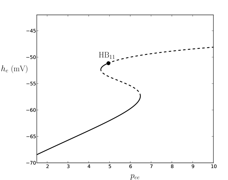
Figure 1: Bifurcation diagram of the spatially homogeneous equilibrium state. Solid lines correspond to stable families and dashed lines to unstable families. The first instability beyond the saddle-node points is a Hopf bifurcation with wave numbers $(1,\,1)$. The periodic orbits are computed in between this point and the second Hopf bifurcation, with wave numbers $(1,\,0)$, shown in figure 3.

In figure 1 a partial bifurcation diagram for the spatially homogeneous equilibrium is shown, constructed by varying only the external input to the excitatory population. A pair of saddle-node bifurcations causes multistability in a parameter interval around $p_{ee}=5$. The top part of the family of equilibria is stable up to the Hopf bifurcation. In fact, this bifurcation is the first of infinitely many, associated with different wave numbers, occurring in a small parameter interval.

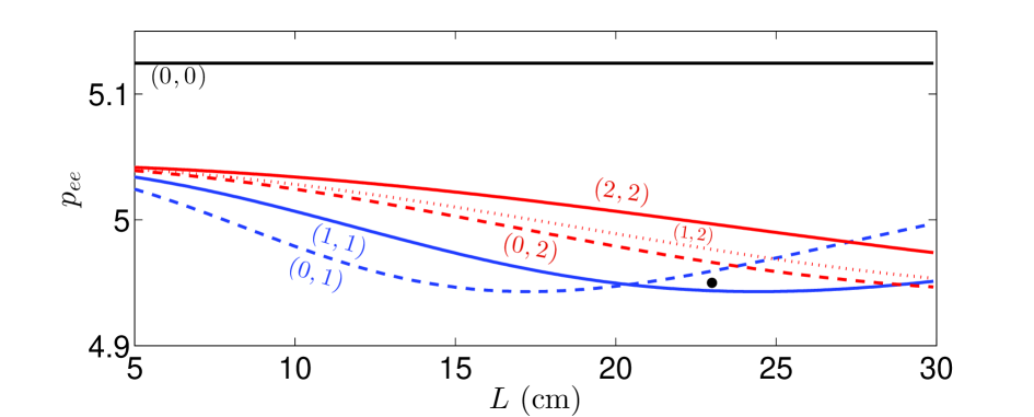
Figure 2: Neutral stability curves for Liley’s mean-field model. Shown are Hopf instabilities with wave numbers up to two (shown between brackets), as the system size $L$ and the external input $p_{ee}$ are varied. All other parameters are chosen as in table 1. The periodic orbit shown in figure 4 was computed at a system size and input parameter represented by the black dot.

Which wave number turns unstable first is determined by the system size, as can be seen from the neutral stability curves in figure 2. Each of the curves shown divides the two parameter plane into regions where perturbations with the specified wave numbers grow or decay. Below the union of these curves, only stable equilibrium solutions are expected to exist. As the system size increases, the wave numbers of the leading instability increase as well, while the length scale of the leading instability saturates at about $16$(cm), and its period around $100$(ms), in the alpha range. At our current system size, $L=23\,\text{(cm)}$, the primary instability has one sinusoidal oscillation in both spatial directions, i.e. it has wave numbers $(1,\,1)$ and thus satisfies both periodic and homogeneous Dirichlet boundary conditions.

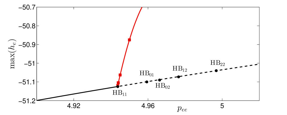
Figure 3: Detail of the bifurcation diagram around the first Hopf bifurcation, on the top branch of figure 1. The solid, black curve corresponds to a stable equilibrium, the dashed black curve to an unstable equilibrium and the red curve to a stable, spatially inhomogeneous periodic orbit. For the latter, the maximum of $h_{e}$ at $(x,\,y)=(L/4,\,L/4)$ is plotted. Red squares correspond to computed periodic orbits and the red line has been added for visibility. Black dots denote Hopf bifurcations for wave numbers up to two, indicated by the subscripts.

When increasing the forcing, $p_{ee}$, at this fixed system size, we cross infinitely many Hopf bifurcations with increasing wave numbers, accumulating at $p_{ee}\approx 5.04$. Those with wave numbers up to two are shown in the detailed bifurcation diagram 3. The red curve in this diagram denotes the standing square periodic solution that emanates from the leading Hopf bifurcation. Snapshots of this solution are shown in figure 4. This close to the bifurcation point, the pattern still looks very much like the sinusoidal eigenmode, and has a period of $98$(ms).

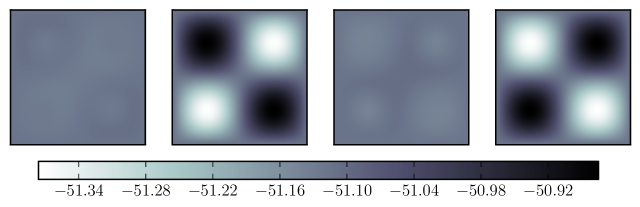
Figure 4: Snapshots of the standing square solution at $p_{ee}=4.95$. Displayed is the excitatory membrane potential ($h_{e}$) at 24.6 ms intervals. The grey scale is in mV.

If we increase the forcing beyond the accumulation point of Hopf bifurcations, complex spatio-temporal dynamics is observed. Figure 5 shows a transient, produced by perturbing the unstable equilibrium along the unstable eigenvector involved in the leading stability. Rings are forming around the four extrema of the sinusoidal pattern, corresponding to a difference in the phase of the oscillation. At the same time, the frequency of the oscillation at the centres increases. We conjecture, that this process will lead to the formation of “hot spots” seen in the onset of gamma band activity in this model bojak2007 . In ongoing work, we attempt to compute periodic solutions that exhibit hot spots. The standing square orbit may well show the initial stage of spot formation, but we may need to track the the attracting solution through a sequence of bifurcations, in which the behaviour becomes increasingly localized.

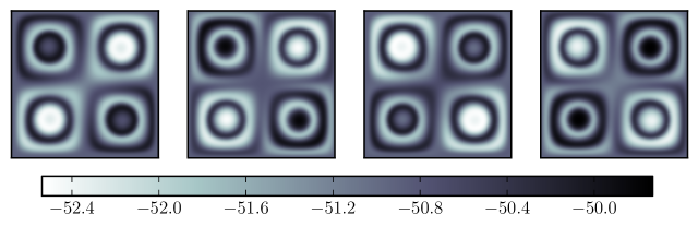
Figure 5: Snap shots the excitatory membrane potential, perturbed away from the equilibrium at $p_{ee}=5.1$ along the unstable eigenmode with wave numbers $(1,\,1)$. The snapshots are $24$(ms) apart. In this transient motion, the frequency of the oscillation at the centre of the four $L/4\times L/4$ squares increases, while rings form around them.

5 Conclusion

We report here on spatially inhomogeneous, time-periodic solutions to a full-fledged, PDE-based mean-field cortex model. To the best of our knowledge, ours is the first attempt to compute such nonlinear invariant solutions for this class of models. The computation is challenging because of the large number of degrees of freedom in the discretized system, the strong nonlinearities and the symmetries of the system that complicate the bifurcation diagram.

This is only the first step in uncovering the dynamical repertoire of the PDE-based model. In ongoing work, we will continue the periodic orbit in the external forcing, and examine its role in the transition from smooth oscillations to localized hot spots and travelling waves. There is mounting evidence, based on Voltage Sensitive Dye (VSD) experiments, that such coherent structures pay a role in information processing (e.g. muller2013 ).

A combination of experimental work and predictive modelling should help us gain insight in the role the cortex plays in high-level brain functioning, as well as in the generation of pathological states such as spreading depression and epileptic seizures. Thus, through this work we hope to contribute indirectly to the better understanding and, hopefully, future treatment of, these common diseases. This noble goal attracts many researchers from different areas of research, not in the last place Hilda Cerdeira, to whose live and work this special issue is devoted.

References

- (1) P. Nunez, R. Srinivasan, Electric Fields of the Brain. The Neurophysics of EEG, 2nd Edition, Oxford University Press, Oxford, 2006.
- (2) D. T. J. Liley, I. Bojak, M. P. Dafilis, L. van Veen, F. Frascoli and B. L. Foster, Bifurcations and state changes in the human alpha rhythm: Theory and experiment, in Modelling phase transitions in the brain, Springer Series in Computational Neuroscience 4, 2009.
- (3) E. Rolls, T. Webb and G. Deco, Communication before coherence, Cogn. Neurosci. 36 (2012) 2689–2709.
- (4) E. Izhikevich, G. Edelman, Large-scale model of mammalian thalamocortical systems, PNAS 105 (2008) 3593–3598.
- (5) G. Deco, V. K. Jirsa, P. A. Robinson, M. Breakspear and K. Friston, The dynamic brain: from spiking neurons to neural masses and cortical fields, PLoS One 4 (2008) e1000092.
- (6) D. A. Pinotsis, M. Leite and K. J. Friston, On conductance-based neural field models, Frontiers Comp. Neurosci. 7 (2013) 1–9.
- (7) H. R. Wilson and J. D. Cowan, A mathematical theory of the functional dynamics of cortical and thalamic nervous tissue, Kybernetik 13 (1973) 55–80.
- (8) H. G. E. Meijer and S. Coombes, Travelling waves in models of neural tissue: from localized structures to periodic waves, EPJ Nonlin. Biomed. Phys. 2:3.
- (9) P. C. Bressloff, Spatiotemporal dynamics of continuum neural fields, J. Phys. A 45 (2012) 033001.
- (10) D. T. J. Liley, P. J. Cadusch and M. P. Dafilis, A spatially continuous mean field theory of electrocortical activity, Network: Comput. Neural Syst. 13 (2002) 67–113.
- (11) I. Bojak and D. T. J. Liley, Modeling the effects of anesthesia on the electroencephalogram, Phys. Rev E 71 (2005) 041902.
- (12) K. R. Green and L. van Veen, Open-source tools for the dynamical analysis of Liley’s mean-field cortex model, J. Comput. Sci. in press.
- (13) I. Bojak and D. T. J. Liley, Self-organised 40Hz synchronization in a physiological theory of EEG, Neurocomputing 70 (2007) 2085–2090.
- (14) A. Stepanyants, L. M. Martinez, A. S. Ferecskó, Z. F. Kisvárday and C. F. Stevens, The fractions of short- and long-range connections in the visual cortex, PNAS 106 (2009) 3555–3560.
- (15) F. Frascoli, L. van Veen, I. Bojak, D. Liley, Metabifurcation analysis of a mean field model of the cortex, Physica D 240 (2011) 949–962.
- (16) S. Coombes, Large-scale neural dynamics: Simple and complex, Neuroimage 52 (2010) 731–739.
- (17) E. Knobloch and M. Silber, Hopf bifurcation with symmetry. In Bifurcation and Symmetry, International Series of Numerical Mathematics 104 241–253; eds. E. L. Allgower, K. Böhmer and M. Golubitsky, Birkhäuser 1992.
- (18) S. Balay, J. Brown, K. Buschelman, W. D. Gropp, D. Kaushik, M. G. Knepley, L. M. Curfman, B. F. Smith, H. Zhang, http://www.mcs.anl.gov/petsc PETSc Web page (2012).
- (19) Source code available from http://bitbucket.org/kegr/mfm
- (20) P. Ashwin, K. Böhmer and M. Zhen, A numerical Liapunov-Schmidt method with applications to Hopf bifurcation on a square, Math. Comp. 64 (1995) 649–670.
- (21) L. E. Muller, A. Reynaud, F. Chavane and A. Destexhe, Propagating waves structure spatiotemporal activity in visual cortex of the awake monkey, BMC Neuroscience 14(Suppl. 1):O8.