Communication and Measurement

James P. Gordon

Rumson, NJ

Abstract

I discuss the process of measurement in the context of a communication system. The set- ting is a transmitter which encodes some physical object and sends it off, a receiver which measures some property of the transmitted physical object (TPO) in order to get some in- formation, and some path between the transmitter and the receiver over which the TPO is sent. The object of the game here is to characterize the TPO, either as an end in itself (research), or to examine its potential for information transmittal (communication). If the TPO is a ’small’ object then quantum mechanics is needed to play this game. In the course of this work, I hope to broaden the concept of measurement in quantum mechanics to in- clude noisy measurements and incomplete measurements. I suggest that quantum density operators are logically associated with the transmitter and some portion of the path, and that quantum measurement operators are logically associated with the rest of the path and the receiver. Communication involves the overlap of a density operator and a measurement operator. That is, the fundamental conditional probability of the communication process is given by the trace of the product of a density operator and a measurement operator.

Preface

In late 2002 Jim Gordon handed me a first draft of this manuscript, proposing that I help him turn it into a paper. In the 1960s, while working for Bell Laboratories, Jim wrote some of the very first papers on quantum communications, essentially giving birth to that important field. Initially, he was interested in exploring the ways in which Shannon’s results regarding information capacity could be extended in order to account for the constraints imposed by quantum physics [1, 2, 3]. He was also interested in the theory of quantum measurement and published one of the first papers on the subject [4]. In the 1970s, however, Jim drifted away from quantum communications as his main interests shifted to other areas of research. It was only after his retirement from Bell Laboratories in the late 1990s that he re-engaged with quantum communications, returning to problems that he hadn’t resolved in the first round. Jim had not been following the literature that had accumulated on the subject in the interim three decades, and after being exposed to some of it during our discussions, he decided not to proceed with the publication of this article. His reasoning was that some of the concepts that he introduced in it had become known over the years.

James P. Gordon died on June 21 2013. In June of the following year, I was asked to give a talk about his contributions to quantum communications at a special symposium held in his memory at the Conference on Lasers and Electro-Optics in San Jose, California [5]. While reviewing the materials, I rediscovered this paper in my files and decided to present it at the symposium [6]. I found that although some of the ideas may have been discussed elsewhere, Jim’s paper also contained important original content. Even more importantly, I realized that his unfinished manuscript offered a unique glance into the workings of a brilliant mind. I also thought that his insightful text would be particularly useful to individuals with some background in optics and quantum physics, who were interested in building up their intuition regarding quantum measurement and communication without resorting to formal or abstract mathematics. With the permission of Jim’s family and colleagues, I decided to make this manuscript public.

Since the author was no longer alive, submission to a peer-reviewed journal did not seem reasonable; instead, posting the manuscript on arxiv seemed to be the most natural choice. What you will find in what follows is the last existing version of Jim’s original text from 2006, retyped without any (intentional) changes, except for the correction of a few obvious typos. It is possible that some unintentional errors were introduced in the process of retyping, and hence the original PDF can be found at http://www.eng.tau.ac.il/~shtaif/jpgcnm.pdf. The posting of this retyped version on arxiv was necessary because arxiv functions as an archival journal, which means that the article can conveniently be cited in future work. Those who find typos in the retyped manuscript are encouraged to contact me at shtaif@eng.tau.ac.il, so that new corrected versions can be posted.

Introduction

The subject of measurement has a long history. It describes how one sees things. All of the problems that come up in this fundamental area have not yet been satisfactorily solved. In particular, the role of the observer (e.g.,you) has never been satisfactorily integrated into the quantum theory. Quantum mechanics arose because the classical theory could not account for the results of laboratory experiments on ’small’ objects like atoms, nor could it account for the spectrum of black body radiation. In graduate school I learned that if an object were prepared in a quantum state $|\psi\rangle$ and one made a measurement of some observable (measurable quantity) $\mathbf{A}$, with possible values $[a]$, the result would be some particular value $a$ with probability $|\langle a|\psi\rangle|^{2}$. This prescription is in accord with the uncertainty principle. It envisages a ”pure” state of the object and an ”exact” measurement of the observable $\mathbf{A}$, and yet the measurement result is often not certain. This scenario fits in with our picture of a communication system. The transmitter prepares the system in the state $|\psi\rangle$ and the receiver measures the observable $\mathbf{A}$ and gets the value $a$. In the real world, of course, the transmitter often cannot put the system in a pure state, the receiver often cannot make an exact measurement, and the transmission path often adds some uncertainty to the result. In other words, the transmitter, the path, and the receiver can each add noise to the system. The more general idea of simultaneous inexact measurements of non-commuting observables was introduced in 1965. In theory, this typically involves coupling the received TPO to an auxiliary system whose initial quantum state is known, followed by exact measurement of a set of commuting observables of the combination. In the case of two non-commuting observables it can also be thought of as a minimally invasive incomplete measurement of one observable followed by an exact measurement of the other. In this work I will try to give a logical picture of the communication process, and of how measurements fit into this picture.

The Model

Figure 1 shows the components of our model communication system. It consists of a transmitter, which sends out some TPO coded according to the transmitter knob setting $t$. The TPO then follows the path to the receiver, during which voyage it may be corrupted by some noise or be otherwise affected. The receiver makes a measurement of some property of the TPO, getting a meter reading $r$. The ability of the system to transmit information is governed by the conditional probability distribution $P_{RT}(r/t)$, defined as the probability that the receiver’s meter reading is $r$ given that the transmitter’s knob setting is $t$. Subscripts on the probability distributions indicate locations, while their arguments give values. The knob settings and the meter readings may be multidimensional. They may, for example, correspond to some set of observables of the TPO. Since the meter always reads some value, the values of $P_{RT}(r/t)$ when summed over $r$ must equal unity.

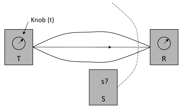
Fig. 1: Cartoon of the model communication system.

We want to know the properties of the TPO, as they are needed to design the best transmitter and/or receiver. The problem then becomes how to describe the TPO somewhere (anywhere) along the transmission path. To deal with this, we draw a surface $S$ cutting the transmission path, and ask how the conditional probability distribution $P_{RT}(r/t)$ depends on the properties of the TPO at $S$. This model covers most if not all laboratory experiments, where the researcher wants to find something new about the nature of things. He/she builds an apparatus which has knobs and meters, and works to try to describe what he/she is looking at. He/she may try to minimize the random disturbances introduced by the transmission path. Sometimes, however, such ’random’ disturbances turn out to be important. The model also applies to communication systems, where the engineer/scientist tries to de- sign the transmitter and receiver in order to maximize the data rate, based on what he/she thinks are the properties of the TPO and the transmission path. Most modern communi- cation systems use electromagnetic fields sent through transmission lines or through space. The TPO in this case might be the field received during some finite segment of time. In the case of astronomy and similar endeavors, where the transmitter is beyond our control, we can call it Nature, or God, as we like. In such a case, if we know something about the properties of the path and the properties of the TPO, we can try to find out something about the transmitter. Another source of corruption of a signal is inter-symbol interference (ISI), where for example neighboring TPOs interfere with each other. I will not deal with this problem, as it is a practical rather than a fundamental issue.

Analysis

So how do we treat this communication problem? The classical answer envisions the possibility of a complete and exact description of the TPO at $S$ by some set of real parameters $s$, so that the conditional probability appears in the form

$$P_{RT}(r/t)=\sum_{s}P_{RS}(r/s)P_{ST}(s/t).$$ (1)

Here, $P_{ST}(s/t)$ is the probability that the TPO at $S$ is in the state $s$ given that the transmitter setting was $t$, while $P_{RS}(r/s)$ is the probability that the receiver records the value $r$ given that the TPO was in the state $s$ at the location $S$. The sum over $r$ of $P_{RS}(r/s)$ and the sum over $s$ of $P_{ST}(s/t)$ both equal unity, so that the sum over $r$ of $P_{RT}(r/t)$ is also unity. Quantum mechanics was invented because this prescription often does not work. Quantum mechanics envisions pairs of conjugate observables (measurable quantities), such that it is not possible to determine a precise value for each at the same time. This is Heisenberg’s uncertainty principle. The canonical example is the position and momentum of a single particle. TPO’s are described by state vectors $|t\rangle$ if they are in pure quantum states, or more generally by density operators $\rho(t)$ whether they are in pure states or in incoherent mixtures of pure states. Here $t$ represents some parameter set that specifies the density operator. Density operators are Hermitian and non-negative, normalized to unit trace. That is, density operators must satisfy the relation

$$\mathrm{Trace}\big{(}\rho(t)\big{)}=1.$$ (2)

Representations of density operators are Hermitian matrices whose elements are formed using the eigenstates of some complete set of commuting observables of the TPO. The diagonal elements of any such representation are non-negative, sum to the trace of $\rho$ and therefore to unity, and are generally acknowledged to form a probability distribution for the exact measurement of those observables. It is of note that such eigenstates need not be possible state vectors of the TPO. For example, the position $x$ of a single one-dimensional particle has eigenstates $|x\rangle$ which can be used to form the representation $\langle x|\rho|x^{\prime}\rangle$ of a particle in the state $\rho$. The diagonal elements $\langle x|\rho|x\rangle$ of this representation give the probability distribution for the observable $x$ of the particle. The eigenstates of $x$ are not possible states of the particle since their norm $\langle x|x\rangle$ is infinite, but they do form a complete set since $\int{\rm d}x|x\rangle\langle x|+\mathbf{I}$, where $\mathbf{I}$ is the identity operator. I will come back to this point later.

In our model communication system, the transmitter prepares the TPO, and sends it off on the path to the receiver. It arrives at the location $S$ described by a density operator, which we will label $\rho_{ST}(t)$, dependent on the transmitter setting $t$ and on the properties of the path from the transmitter to the location $S$. It can have no dependence on the receiver or on the part of the path from $S$ to the receiver. Since there are a number of different possible representations of $\rho_{ST}(t)$, there is no unique set of values $s$ at $S$ as there is in the classical picture. This is one of the important aspects of quantum mechanics. The receiver is a measuring device. It measures some set of observables of the TPO, either well or badly, and gets a result $r$ with the probability $P_{RT}(r/t)$. The most general way of describing this process would seem to consist of a relation in the form

$$P_{RT}(r/t)=\mathrm{Trace}\big{(}\sigma_{RS}(r)\rho_{ST}(t)\big{)},$$ (3)

where the operator $\sigma_{RS}(r)$ of Eq.(3) is a measurement operator. For example, the probability distribution formed by the diagonal elements $\langle r|\rho|r\rangle$ of any representation of the TPO can be represented in the form of Eq (3), with $\sigma(r)=|r\rangle\langle r|$. In our communications milieu, this would be the the result of an exact measurement of the set of commuting observables that creates the representation. The measured value, $r$, would be the set of eigenvalues of that set of observables for the eigenstate $|r\rangle$.

I call the operator $\sigma_{RS}(r)$ of Eq.(3) a measurement operator since it portrays the receiver’s role in the communication process. My thesis here is that measurement operators may be given a broad scope, limited only by a few necessities. A measurement operator depends only on the receiver’s result $r$ and on the properties of the path from $S$ to the receiver. It can have no dependence on the transmitter setting $t$ or on the part of the path from the transmitter to $S$. The receiver may know or guess the properties of the TPO being sent, and it may also know of any restrictions placed on the scope of the transmitter’s choices, but it knows nothing a priori about which of these choices has been made.

There are two basic requirements for any measurement operator. First, since $P_{RT}(r/t)$ must be a non-negative real number for any possible density operator representing the TPO, it follows that $\sigma_{RS}(r)$ must be Hermitian and non-negative, just as is a density operator. Second, since $P_{RT}(r/t)$ is a probability distribution, summing over $r$ to unity, the measurement operators must sum over $r$ to the identity operator. That is, the measurement operators must satisfy the relation

$$\sum_{r}\sigma(r)=\mathbf{I}.$$ (4)

The measurement operators must therefore form a complete set for the TPO. Their properties need not be otherwise restricted. In our discussion of a 1D particle, the operator $|x\rangle\langle x|$ is an example of a measurement operator, even though it cannot be a density operator. More precisely, it represents a limiting case of a real world measurement operator, since a truly exact measurement of a continuous observable such as $x$ is beyond our capacity. The division of quantum operators into two types, namely density operators which have unit trace and measurement operators which satisfy a completeness relation, makes sense to me because there are examples of each which do not fit into the other category.

In the early days of quantum mechanics, measurements were discussed only in the context of representations of the density operator, thus implicitly involving only exact measurements of complete sets of commuting observables. As I understand it, Heisenberg arrived at the uncertainty principle by considering the measurement process, but the result was viewed only through the properties of the density operator. More recently, with the advent of lightwave communications, the scope of measurement operators was broadened to include inexact simultaneous measurements of non-commuting observables, necessarily inexact because the uncertainty principle forbids simultaneous exact measurements of such observables. This type of measurement involves over-complete sets of measurement states, such as the coherent states of the simple harmonic oscillator. Here I propose to take the measurement operator concept one step further, that is, to broaden the scope of measurement operators to include any operators $\sigma_{RS}(r)$ that satisfy the two basic requirements. It may not be easy or even possible to imagine a device to realize every such measurement operator, but it should be possible to devise a measurement operator to correspond to any imaginable device for measuring any set of observables of a TPO. Some representative examples are discussed below.

If the path is noisy, the density operators and measurement operators representing the TPO will change for different positions of $S$ along the path, but the probability $P_{RT}(r/t)$ must re- main independent of the location of $S$. This condition leads to some interesting relationships, as we shall see later.

If the effects of the path are negligible, and the TPO at $S$ is actually in a pure quantum state $|\psi\rangle$ then $\rho_{ST}(\psi)=|\psi\rangle\langle\psi|$. If in addition the receiver can accurately measure an observable $\mathbf{A}$ whose eigenvalues are $[a]$, then $\sigma_{RS}(a)=|a\rangle\langle a|$. Thus we come to my graduate school result, namely that the probability of the measurement result a given the quantum state $|\psi\rangle$ is

$$P_{RT}(a/\psi)=\mathrm{Trace}\big{(}\sigma_{RS}(a)\rho_{ST}(\psi)\big{)}=\mathrm{Trace}\big{(}|a\rangle\langle a||\psi\rangle\langle\psi|\big{)}=|\langle a|\psi\rangle|^{2}.$$ (5)

The description of the TPO at $S$ in terms of a quantum density operator automatically satisfies the uncertainty principle with respect to the ability of the transmitter to ascribe values to the observables of the TPO. Likewise, the description of the measurement process at $S$ in terms of a quantum measurement operator automatically satisfies the uncertainty principle with respect to the ability of the receiver to measure these values. The point is that neither the transmitter nor the receiver can ever know more about the TPO than the uncertainty principle permits. In the communication process, the uncertainty principle applies independently to the preparation and to the measurement of any TPO.

There is considerable overlap in the realms of density operators and measurement operators. There are differences, however. For example, measurements of only one of a non-commuting conjugate pair of observables correspond to measurement operators whose traces are infinite, so they cannot serve as density operators.

This completes our brief formal analysis. Density operators are discussed in most texts on quantum mechanics. In the rest of this paper, I will discuss various examples to give substance to the idea of measurement operators. For simplicity, I will deal with TPO’s in the form of simple harmonic oscillators (SHO)s, and two level systems (TLS)s. Linear fiber optical communication systems can be modelled by SHOs transmitted at a rate given by the system bandwidth. In the modern parlance of quantum computation, TLSs are examples of qbits. Thus there is some substance to this work. Bold face will be used for operators, but not for values. The context can also help to distinguish values from operators.

The simple Harmonic Oscillator

The classical picture of the SHO envisions the possibility of exact prescription and of exact measurement of both the position and momentum of a particle in a harmonic potential well. From the standpoint of communications, this implies that the information transfer possible using a single SHO of finite energy is limited only by noise. As we know, this classical picture runs into fatal trouble trying to explain things such as the law of black body radiation. The quantum picture of the SHO is more complicated, and is really quite counter-intuitive. The conjugate variables position and momentum are represented by non-commuting operators. The result is a ladder of energy states separated by the quantum of energy, the lowest of which has an energy one-half quantum above the bottom of the potential well. Either position or momentum can still be prescribed and/or measured as exactly as one pleases, but only at the expense of greater and greater uncertainty, and therefore greater expected energy, in the conjugate variable. Communication, with an energy constraint, is thereby limited even in the absence of noise. Elements of the quantum theory of the SHO are reviewed in Appendix A.

The SHO provides a fertile ground for studying the communications problem. The transmitter may be able to send SHOs in either energy states or minimum uncertainty ’coherent’ states. The path may involve either loss or gain, or both. The receiver may measure energy, or position or momentum, or both. I will examine a number of these possibilities.

First, let us look at the case where the SHOs are encoded and measured by energy. Suppose that the transmitter can emit SHO’s with exactly $N$ energy quanta. Suppose also that the path is purely lossy, and that the receiver can measure the exact number of quanta in the received SHO. The probability that the receiver measures $M$ quanta given that the transmitter sent $N$ quanta is given by the binomial distribution

$$P_{RT}(M/N)=C_{M}^{N}(p_{RT})^{M}(1-p_{RT})^{N-M}\equiv B_{M}^{N}(p_{RT}),$$ (6)

where $C_{M}^{N}$ is the binomial coefficient, while $p_{RT}$ is the probability that a quantum will survive the loss in the path between the transmitter and the receiver. The last expression defines the binomial form $B_{M}^{N}(p_{RT})$.

The energy states $|n\rangle$ are labelled by the number of quanta, and comprise a complete set, so they can also be used as measurement states. They satisfy the relations $\langle n|m\rangle=\delta(n,m)$ and $\sum|n\rangle\langle n|=\mathbf{I}$.

If we put the surface $S$ immediately in front of the receiver, the density operator representing the transmitted SHO will reflect the binomial probability distribution, while the measurement operator will reflect the exact number of received quanta. It is pretty clear that the density and measurement operators in this example are given by

$$\rho_{ST}(N)=\sum_{n}B_{n}^{N}(p_{RT})|n\rangle\langle n|\hskip 56.9055pt\sigma_{RS}(M)=|M\rangle\langle M|,$$ (7)

since $B_{n}^{N}(p_{RT})$ is the probability the n quanta reached the receiver given that $N$ quanta were sent. In this case, the conditional probability $P_{RT}(M/N)$ of Eq.(6) can be written as $\langle M|\rho_{ST}(N)|M\rangle$, which is one of the diagonal elements of the density operator written in the number representation. This accords with the standard recipe for measurements in quantum mechanics. However, in our extended view of measurement operators, we can equally well put the surface $S$ immediately after the transmitter. In this case the density operator for the sent SHO represents a pure state of $N$ quanta, and so the binomial distribution must therefore be represented in the measurement operator. The density and measurement operators transform to

$$\rho_{ST}(N)=|N\rangle\langle N|\hskip 56.9055pt\sigma_{RS}(M)=\sum_{n}B_{M}^{n}(p_{RT})|n\rangle\langle n|.$$ (8)

This relation is an example of an inexact measurement operator. It follows since $P_{RT}(M/N)$ must be independent of the location of the surface $S$, and it makes sense since $B_{M}^{n}(p_{RT})$ is the probability that $M$ quanta reached the receiver given that $n$ quanta were sent.

In more generality, we can locate $S$ anywhere between transmitter and receiver. In this case Eqs.(7) and (8) change to

$$\rho_{ST}(N)=\sum_{n}B_{n}^{N}(p_{ST})|n\rangle\langle n|\hskip 56.9055pt\sigma_{RS}(M)=\sum_{n}B_{M}^{n}(p_{RS})|n\rangle\langle n|,$$ (9)

where $p_{RS}p_{ST}=p_{RT}$. In these three examples, the prerequisites are satisfied, as they must be. That is, in each case $\mathrm{Trace}(\rho)$ is unity, the sum of $\sigma$ over the measurement results gives the identity operator, and $\mathrm{Trace}(\sigma\rho)$ gives the conditional probability of the measurement result, given the transmitter setting. For example, from Eq.(9) we have

$$P_{RT}(M/N)=\mathrm{Trace}\big{(}\sigma_{RS}(M)\rho_{ST}(N)\big{)}=\sum_{n}B_{M}^{n}(p_{RS})B_{n}^{N}(p_{ST})=B_{M}^{N}(p_{RT}),$$ (10)

in accord with Eq. (6). Because all of the density and measurement operators are diagonal in the same (here energy) representation, these results have the form of the classical Eq.(1), with $s=n$, $t=N$, and $r=M$. The role of quantum mechanics is the quantization of the energy. This example however illustrates an important communications limitation imposed by quantum mechanics. Communication using this system is maximized if there is no attenuation in the path. In this case Eq.(6) reduces to $P_{RT}(M/N)=\delta(M,N)$. If the system is only allowed to use SHO’s with energies no greater than $N$ quanta, the information transfer per SHO is limited to $\log_{2}(N)$ bits. There is no way of encoding the SHO’s that exceeds this limit under the same constraint.

As I noted above, the measurement operators are independent of the properties of the transmitter and the portion of the path prior to $S$. Thus for any $\rho_{ST}(t)$, the receiver represented by Eq.(9) would measure $M$ quanta with probability $P_{RT}(M/N)=\sum_{n}B_{M}^{n}(p_{RS})\langle n|\rho_{ST}(t)|n\rangle$. The measurement operators of Eqs. (8) and (9) describe inexact measurements of the number of quanta at $S$, inexact because of the attenuation in the path from $S$ to the receiver.

The basic properties of the distribution $B_{M}^{n}(p)$ as a function of $n$ are

$$\sum_{n}B_{M}^{n}(p)=\frac{1}{p}\hskip 14.22636ptn_{max}\simeq M/p-0.5\hskip 14.22636pt\Delta n\simeq\frac{2.355}{p}\sqrt{M(1-p)+p/2},$$ (11)

where $p<1$, $n_{max}$ is the location of the peak of the distribution, and $\Delta n$ is its full width at half maximum (fwhm), based on the curvature of the peak along with a Gaussian approximation to its shape. The actual distribution is somewhat skewed toward higher values of $n$, but the value of the fwhm is reasonably accurate. For example, if $M=20$ and $p=0.5$, the distribution peak is approximately at $n=39.5$ (the values at $n=39$ and $n=40$ are equal), and the fwhm is approximately 15 (the values nearest to the half maxima are at $n=33$ and $n=48$).

An alternate regime for communication using SHO’s is a coherent system, where phase information as well as amplitude information is used. In quantum mechanics, the simplest such system involves a transmitter emitting SHO’s in minimum uncertainty coherent states, and a receiver using coherent states as measurement states. As discussed in Appendix A, the coherent states are versions of the ground state displaced to other places in the phase space of the SHO. When subject to pure attenuation, it is well known that coherent states remain coherent states as their mean values (signals) decay. When subject to pure gain, it is also well known that enough noise is added to maintain the validity of the uncertainty principle.

Let us see how this situation plays out in our picture of measurements. The density operator corresponding to the pure coherent state $\alpha\rangle$ is denoted $|\alpha\rangle\langle\alpha|$, where $\alpha$ is a complex number which may be thought of as a classical signal. The measurement operator corresponding to the pure coherent state $|\beta\rangle$ is denoted $\pi^{-1}|\beta\rangle\langle\beta|$, where $\beta$ is also a complex number. The difference is due to the normalization required of the two operators. If the transmitter sends the SHO in the state $|\alpha\rangle$, and the path is loss free, the probability that an ideal coherent receiver would record the value $\beta$ is given by $P_{RT}(\beta/\alpha)=\pi^{-1}|\langle\beta|\alpha\rangle|^{2}=\pi^{-1}\exp(-|\beta-\alpha|^{2})$. Thus, with both ideal preparation and ideal measurement in a coherent system, there is uncertainty in the result, having a two dimensional Gaussian distribution that corresponds to an effective single quantum of Gaussian noise.

To see this more clearly, we can generalize the above result. Suppose that the path adds some extra Gaussian noise, and that $S$ is immediately in front of the receiver. The density operator corresponding to signal plus Gaussian noise using the coherent state expansion is given in Appendix B, Eq.(B.11). The same ideal coherent receiver would record the value with the probability

$$P_{RT}(\beta/\alpha) = \frac{1}{\pi^{2}\bar{n}}\int\int{\rm d}^{(2)}(\xi)\exp\left(\frac{|\xi-\alpha|^{2}}{\bar{n}}\right)|\langle\beta|\xi\rangle|^{2}$$ (12)

$$= \frac{1}{\pi(\bar{n}+1)}\exp\left(-\frac{|\beta-\alpha|^{2}}{\bar{n}+1}\right),$$

where $\bar{n}$ is the mean number of noise quanta, and $|\xi\rangle$ represents a coherent state.

For the same conditions, let us put $S$ immediately after the transmitter. Then $\rho_{ST}(\alpha)=|\alpha\rangle\langle\alpha|$ and we need a measurement operator which will reproduce the result of Eq(12). The answer is

$$\sigma_{RS}(\beta)=\frac{1}{\pi^{2}\bar{n}}\int\int{\rm d}^{(2)}(\xi)\exp\left(\frac{|\xi-\beta|^{2}}{\bar{n}}\right)|\xi\rangle\langle\xi|.$$ (13)

Thus, akin to the case of a lossy line with photon numbers being prescribed and measured, a noisy coherent signal and a pure coherent measurement is equivalent to a pure coherent signal and a noisy coherent measurement. One can see from Eq.(12) that this communication process involves an effective minimum of one quantum of Gaussian noise.

In the interest of simplicity, I am not taking into account whatever phase shifts may occur in the path.

Other cases of interest are where the path involves loss or gain. First, consider the case of pure loss, with $S$ immediately in front of the receiver. If the transmitter sends a SHO in the coherent state $|\alpha\rangle$, it will reach the receiver in the coherent state $|\alpha/\sqrt{L}\rangle$, where $L\geq 1$ is the loss. If the receiver then measures the value $\beta$ corresponding to the coherent measurement state $|\beta\rangle$, we get for the conditional probability the result

$$P_{RT}(\beta/\alpha)=\pi^{-1}|\langle\beta|\alpha/\sqrt{L}\rangle|^{2}=\pi^{-1}\exp\left(-|\beta-\alpha/\sqrt{L}|^{2}\right).$$ (14)

This is straightforward, but now what if $S$ is immediately in front of the transmitter? The density operator for the transmitted signal is then just $|\alpha\rangle\langle\alpha|$, and we need to discover the measurement operator. If we rewrite Eq (14) as

$$P_{RT}(\beta/\alpha)=\pi^{-1}\exp\left(-\frac{|\sqrt{L}\beta-\alpha|^{2}}{L}\right),$$ (15)

and compare it with Eqs.(12) and (13), the answer emerges as

$$\sigma_{RS}(\beta)=\frac{1}{\pi^{2}}\frac{L}{L-1}\int\int{\rm d}^{(2)}(\xi)\exp\left(\frac{|\xi-\sqrt{L}\beta|^{2}}{L-1}\right)|\xi\rangle\langle\xi|.$$ (16)

Thus it happens again that an attenuated signal and a pure measurement is equivalent again to a pure signal and a noisy measurement. This is not too surprising, but I was happy to find this result.

The case where the path has pure gain turns out to be the inverse of the case of pure loss. To see this, suppose that $S$ is first placed at the transmitter. Then the density operator for the transmitted SHO is simply $\rho_{ST}|\alpha\rangle\langle\alpha|$. The best we can do in coherent measurements is to use coherent measurement states. So suppose that the measurement operator is $\sigma_{RS}(\beta)=(\pi G)^{-1}|\beta/\sqrt{G}\rangle\langle\beta/\sqrt{G}|$. (Remember that the value $\beta$ is what the receiver records, and that the path has gain $G$.) In this case the conditional probability evaluates to

$$P_{RT}(\beta/\alpha)=\frac{1}{\pi G}\exp\left(|\alpha-\beta/\sqrt{G}|^{2}\right).$$ (17)

When $S$ is moved to the receiver, the measurement operator becomes $\sigma_{RS}(\beta)=\pi^{-1}|\beta\rangle\langle\beta|$, and the density operator necessary to preserve the conditional probability Eq(17) is

$$\rho_{ST}(\alpha)=\frac{1}{\pi(G-1)}\int\int{\rm d}^{(2)}(\xi)\exp\left(\frac{|\xi-\sqrt{G}\alpha|^{2}}{G-1}\right)|\xi\rangle\langle\xi|.$$ (18)

This density operator has the form of signal plus noise, with $\bar{n}=G-1$. This is not too surprising, but it is impressive that the uncertainty principle (which is responsible for the coherent states) also demands the emission of the noise that is well known to accompany gain in a transmission system.

As we have just seen, in the coherent state picture the cases of pure loss and pure gain are intimately related. Normalization aside, the density operator for pure gain with $S$ at the receiver has the same form as the measurement operator for pure loss with $S$ at the transmitter. These are given in Eqs.(18) and (16). The question arises (courtesy of M.S.), does the same apply to the case where number states are used. His answer is yes. From the measurement operator in Eq.(8), one may guess that the density operator for the case of pure gain with $S$ at the receiver, when $N$ photons are sent, would be

$$\rho_{ST}(N)=G^{-1}\sum_{n}B_{N}^{n}(G^{-1})|n\rangle\langle n|,$$ (19)

and this is the correct answer. For example, the mean number of photons predicted by this distribution is $GN+G-1$, which represents the input number multiplied by $G$ plus the $G-1$ photons expected from the spontaneous emission that accompanies the gain.

Since the density operators and measurement operators are independent entities, there are many combinations that can be examined. One that I find pedagogically interesting is to transmit a number state, and measure it using coherent states, with no loss or gain in the path. The result is

$$P_{RT}(\beta/n)=\pi^{-1}|\langle\beta|n\rangle|^{2}=\frac{1}{\pi n!}(\beta\beta^{*})^{n}\exp(-\beta\beta^{*}).$$ (20)

This probability distribution peaks at $|\beta|^{2}=n$ independent of the phase of $\beta$. It is a smoothed measure of how the number states are distributed in the phase space of the SHO.

The Wigner Picture

To visualize these results it is useful to appeal to the Wigner distributions. As discussed in Appendix B, these are quasi-classical distributions in the phase space of the SHO that are isomorphic with the quantum density operators. They differ from classical probability distributions in that for most quantum states, the corresponding Wigner distributions have negative values in various regions of the phase space. For the cases of signal plus Gaussian noise discussed above, however, they are positive definite, and lead to a classical picture of the communications process. Furthermore, they can give a classical description of quadrature squeezed states. I think that it is fair to think of any SHO whose Wigner distribution is positive definite as being in a ’classical’ state.

There are three important features of the Wigner picture. First, as just mentioned, Wigner distributions are isomorphic with quantum density operators, so they can accurately represent quantum states. Second, as also noted in appendix B, the integral over the phase space of the SHO of the product of two Wigner distributions is proportional to the trace of the product of the corresponding two density operators. With a change in the normalization, Wigner distributions can also represent measurement operators. Thus, the crucial conditional probability $P_{RT}(r/t)$ of the communications process can be correctly viewed as the overlap of two Wigner distributions in the phase space, in the form of Eq.(1). Third, of considerable importance to the photonic communications business, the Wigner distribution for the SHO obeys the classical equations of motion, with no quantum corrections. This is true also for linear couplings of the SHO to heat baths, yielding attenuation or gain. For a particle in an anharmonic potential, the Wigner distribution obeys the classical equations of motion to second order in the size of the energy quantum. As a result, the first and second moments of Wigner distributions always behave classically. One must go to third and higher moments to find quantum corrections. Although as far as I know it has not yet been proven, I do not think it is much of a stretch to presume that for photonic propagation in glass fibers, with their weak non-linearity, the Wigner picture yields a very close classical approximation to the exact quantum picture. It does so if an adequate description of the field in the fiber consists of signal plus Gaussian noise, which depends only on first and second moments. This is, for example, why there are no significant quantum corrections to a classical description of soliton propagation in fibers using the Wigner picture.

In essence, the Wigner picture treats the half quantum of zero point field of the SHO as an integral part of a total classical Gaussian noise field. In particular, the zero point field suffers attenuation and/or gain just as do any additional noise fields. This has implications in regard to noise generation from media that attenuate or amplify the field. Attenuators must be noise generators in order to maintain the zero-point field. As it turns out, the spontaneous emission of noise in the Wigner picture is the same for both amplifying and attenuating media. We will see later how this may be rationalized.

Let us look for the Wigner picture of measurement states. The Wigner picture uses the coordinates $(p,q)$ of phase space. If we rewrite the coherent state $|\alpha\rangle$ as $|p,q\rangle$, where $\alpha=(1/\sqrt{2})(q+ip)$, the completeness relation becomes $(1/\sqrt{2})\int{\rm d}p\int{\rm d}q|p,q\rangle\langle p,q|=\mathbf{I}$. Thus, if we use the coordinates of phase space, we find that

$$\sigma(p,q)=(1/\sqrt{2})\rho(p,q).$$ (21)

It follows from Eq. (5) of Appendix B that the Wigner distribution corresponding to a measurement state is

$$W(p,q/\sigma)=\int{\rm d}q^{\prime}\langle q-\frac{1}{2}q^{\prime}|\sigma|q+\frac{1}{2}q^{\prime}\rangle\exp(iq^{\prime}p).$$ (22)

This form works for all measurement operators, including those with in nite trace. For example, the Wigner distribution corresponding to the measurement operator $|q^{\prime\prime}\rangle\langle q^{\prime\prime}|$ is $W(p,q)=\delta(q-q^{\prime\prime})$. This Wigner distribution is not integrable because it is independent of p, but it is nonetheless applicable to the communications problem, since its overlap with the Wigner distribution corresponding to any density operator is finite.

In view of Eq. (21) and Eq. (B.6) of Appendix B, it follows that the basic conditional probability of the communication process can be written in the classical form

$${P_{RT}}(r/t)=\int{\rm d}p\int{\rm d}qW_{RS}(p,q/r)W_{ST}(p,q/t),$$ (23)

where $W_{ST}$ is the Wigner distribution corresponding to the density operator $\rho_{ST}$ and $W_{RS}$ is the Wigner distribution corresponding to the measurement operator $\sigma_{RS}$.

As given in appendix B, the basic Wigner distribution for the SHO corresponding to signal plus Gaussian noise is given by

$$W(p,q/p^{\prime},q^{\prime})=\frac{1}{\pi(2\bar{n}+1)}\exp\left(-\frac{(q-q^{\prime})^{2}+(p-p^{\prime})^{2}}{2\bar{n}+1}\right),$$ (24)

where $\bar{n}$ is the mean number of noise quanta. This is a two dimensional Gaussian centered on the signal $(p^{\prime},q^{\prime})$. Note the extra half quantum of zero-point noise represented in the quantity $2\bar{n}+1$, where $\bar{n}$ is the mean number of noise quanta. The case $\bar{n}=0$ is the Wigner distribution for a coherent state, which consists of a signal plus half a quantum of Gaussian noise.

Consider then the cases of coherent communication discussed above. With a lossy path, and $S$ at the receiver, we have

$$W_{ST}(p_{S},q_{S}/p_{T},q_{T})=\pi^{-1}\exp\big{(}-(q_{S}-q_{T}/\sqrt{L})^{2}-(p_{S}-p_{T}/\sqrt{L})^{2}\big{)}$$ (25)

and

$$W_{RS}(p_{R},q_{R}/p_{S},q_{S})=\pi^{-1}\exp\big{(}-(q_{R}-q_{S})^{2}-(p_{R}-p_{S})^{2}\big{)},$$ (26)

which yields from Eq. (23)

$$P_{RT}(p_{R},q_{R}/p_{T},q_{T})=\frac{1}{2\pi}\exp\left(-\frac{(q_{R}-q_{T}/\sqrt{L})^{2}+(p_{R}-p_{T}/\sqrt{L})^{2}}{2}\right).$$ (27)

In this communication there is an effective one quantum of noise, half of which is associated with the transmitted SHO, and half is associated with the measurement. With the same lossy path, and $S$ at the transmitter, we get

$$W_{ST}(p_{S},q_{S}/p_{T},q_{T})=\pi^{-1}\exp\big{(}-(q_{S}-q_{T})^{2}-(p_{S}-p_{T})^{2}\big{)}$$ (28)

and

$$W_{RS}(p_{R},q_{R}/p_{S},q_{S})=\frac{L}{\pi(2L-1)}\exp\left(-\frac{(q_{R}\sqrt{L}-q_{S})^{2}+(p_{R}\sqrt{L}-p_{S})^{2}}{2L-1}\right),$$ (29)

which again leads to Eq. (27) via Eq. (23). Looking back up the path, the measurement becomes noisy in order to maintain the same signal to noise ratio. Similar results apply to the case where the path has gain.

States of the SHO which are quadrature squeezed versions of signal plus additive Gaussian noise also have positive definite Wigner densities, and so we can think of them as classical states. In recent years there has been much interest in such squeezed states of the radiation field, and while they have proven difficult to make, some squeezing has been achieved. Most attention has been focused on squeezed versions of the vacuum state. A substantial problem is that the squeezed vacuum reverts to the zero point field when it is attenuated. In the Wigner picture, this is simply because the initial squeezed field is attenuated, while the zero point field grows to replace it.

The Wigner density for the quadrature squeezed vacuum has the form

$$W(p,q)=\pi^{-1}\exp\big{(}-\eta q^{2}-p^{2}/\eta\big{)},$$ (30)

where $\eta$ is a positive real parameter. If $\eta$ is greater than one, the state is squeezed in the $q$ direction and enlarged in the $p$ direction, while the reverse is true if $\eta$ is less than one. All squeezed vacuum states take up the same area in the phase space, as required by the uncertainty principle. The propagation of a squeezed vacuum state in a lossy path can be determined from the foregoing. If a transmitter emits a SHO in a squeezed vacuum state, and an ideal coherent detector lies at the end of the path, then if we locate $S$ at the transmitter, we have

$$W_{ST}(p_{S},q_{S}/t)=\pi^{-1}\exp\big{(}-\eta q_{S}^{2}-p_{S}^{2}/\eta\big{)}.$$ (31)

Because the state preparation and the state measurement are independent processes, the measurement is again described by the Wigner density of Eq. (29). Thus we get, according to Eq. (23),

$$P_{RT}(p_{R},q_{R}/t) = \frac{L}{\pi\sqrt{(2L-1+\eta^{-1})(2L-1+\eta)}}\times$$ (32)

$$\exp\left(-\frac{Lq_{R}^{2}}{2L-1+\eta^{-1}}-\frac{Lp_{R}^{2}}{2L-1+\eta}\right).$$

If we now move $S$ to the receiver, where the measurement is described by Eq. (26), in order to preserve Eq. (32) the Wigner density of the transmitted state evaluates to

$$W_{ST}(p_{S},q_{S}/t) = \frac{L}{\pi\sqrt{(L-1+\eta^{-1})(L-1+\eta)}}\times$$ (33)

$$\exp\left(-\frac{Lq_{S}^{2}}{L-1+\eta^{-1}}-\frac{Lp_{S}^{2}}{L-1+\eta}\right).$$

One can see how the field transforms from the initial squeezed state at $L=1$ to the zero point field when $L\gg 1$. The field described by Eq. (33) can be decomposed into the sum of two fields, one, the incident squeezed field, decaying with $p,q\propto\sqrt{1/L}$ and the other, the zero point field, growing as a result of the combination of emission and absorption, with $p,q\propto\sqrt{1-1/L}$.

Incomplete measurements

So far this discussion of the SHO has been concerned with what we may call complete measurements, which may be de ned as those measurements that leave no residual information about the transmitter setting. There is another class of measurements, incomplete measurements, which can leave such information. A canonical example of an incomplete measurement is given by the measurement operator

$$\sigma_{RS}(q_{R}) = \sqrt{\frac{\eta}{\pi}}\exp\big{(}-(\eta(q_{R}-\mathbf{q})^{2}\big{)}$$ (34)

$$= \sqrt{\frac{\eta}{\pi}}\int{\rm d}q\exp\big{(}-(\eta(q_{R}-q)^{2}\big{)}|q\rangle\langle q|,$$

where the second form has been expanded in the position representation. The result of such a measurement is

$$P_{RT}(q_{R}/t) = \mathrm{Trace}\big{(}\sigma_{RS}(q_{R})\rho_{S}T(t)\big{)}$$ (35)

$$= \sqrt{\frac{\eta}{\pi}}\int{\rm d}q\exp\big{(}-(\eta(q_{R}-q)^{2}\big{)}\langle q|\rho_{ST}|q\rangle.$$

This result bespeaks a measurement of the position variable $\langle q|\rho_{ST}|q\rangle$ of $\rho_{ST}$ with an accuracy controlled by the value of the real positive parameter $\eta$. Some information about the transmitted SHO may still be available after such a measurement.

Some discussion is merited here. Since the measurement operator of Eq. (34) has an infinite trace, it cannot be renormalized into a density operator. For any real world measuring device, however, some limitation on the momentum variable $p$ is always present, so one may argue that the trace of any real world measurement operator must be finite. This is surely so, but I believe that it leads only to analytical complexity. Also in the real world, the TPO after the measurement may be left in a variety of states, depending on the measuring device. It may be consumed, or not. There is a class of measurements, appropriately called non-demolition measurements, which do not destroy the TPO. After any non-demolition measurement, the density operator representing the TPO must reflect the result of the measurement $r$ as well as the original transmitter setting $t$. Hence it must change. I denote a minimally invasive measurement giving the result $r$ as one that leaves the TPO in the state

$$\rho_{RT}(t,r)=\big{(}P_{RT}(r/t)\big{)}^{-1}\sqrt{\sigma_{RS}}\rho_{ST}\sqrt{\sigma_{RS}}.$$ (36)

In this relation, $\rho_{RT}(t,r)$ is the residual density operator, which now depends on both the transmitter setting $t$ and the measurement result $r$. Since any measurement operator $\sigma_{RS}(r)$ is Hermitian and non-negative, it has a Hermitian and non-negative square root, which is what is meant in Eq. (36). To find this square root, one can diagonalize the measurement operator and then take the positive square root of each diagonal element. The relation (36) is the simplest way of creating a new density operator dependent on the original density operator and on the measurement operator. It is a generalization of previous formulations in that the measurement operator is a generalization of previous work. Note that if the measurement is complete, the TPO is left in a state which depends only on the measurement result. To take a simple example, if the TPO is a SHO, an ideal coherent measurement has the measurement operator $\pi^{-1}|\beta\rangle\langle\beta|$ whose square root is $\pi^{-1/2}|\beta\rangle\langle\beta|$. According to Eq. (36) a SHO may at best be left, after the measurement, in the coherent state $|\beta\rangle\langle\beta|$, which depends only on the measurement result, and not at all on the transmitter setting.

If some information about the transmitter setting is left in the new density operator, it may be harvested by a subsequent measurement. Suppose that we have two sequential measuring devices $R_{1}$ and $R_{2}$. A minimally invasive measurement by $R_{1}$ giving a result $r_{1}$ leaves a TPO in a state described by

$$\rho_{R_{1}T}(t,r_{1})=\big{(}P_{R_{1}T}(r_{1}/t)\big{)}^{-1}\sqrt{\sigma_{R_{1}S}}\rho_{ST}\sqrt{\sigma_{R_{1}S}}.$$ (37)

A subsequent measurement on the same TPO having the measurement operator $\sigma_{R_{2}R_{1}}(r2)$ gives the result

$$P_{R_{2}R_{1}}(r_{2}/t,r_{1})=\mathrm{Trace}\big{(}\sigma_{R_{2}R_{1}}(r_{2})\rho_{R_{1}T}(t,r_{1})\big{)}.$$ (38)

Using the relations (37) and (38), we can obtain

$$P_{RT}(r_{2},r_{1}/t)=P_{R_{2}R_{1}}(r_{2}/t,r_{1})P_{R_{1}T}(r_{1}/t)=\mathrm{Trace}\big{(}\sigma_{RS}(r_{1},r_{2})\rho_{ST}(t)\big{)}.$$ (39)

where in the second form

$$\sigma_{RS}(r_{1},r_{2})=\sqrt{\sigma_{R_{1}S}(r_{1})}\sigma_{R_{2}R_{1}}(r_{2})\sqrt{\sigma_{R_{1}S}(r_{1})}$$ (40)

is the measurement operator corresponding to the two sequential measurements. If the either measurement is complete, then the combined measurement is also complete.

To take a simple example, suppose that the TPO is a SHO, that the first measurement is an incomplete measurement of position as given by Eq. (34), and that the second is an exact measurement of momentum, given by $\sigma_{R2R1}(pR)=|p_{R}\rangle\langle p_{R}|$. With a little work, we can show that this combined measurement is equivalent to one using squeezed states as measurement states. The measurement operator for the combined measurement, according to the relation (40) is

$$\sigma_{RS}(q_{R},p_{R})=\sqrt{\frac{\eta}{\pi}}\left(\exp\left(-\frac{\eta}{2}(q_{R}-\mathbf{q})^{2}\right)|p_{R}\rangle\langle p_{R}|\exp\left(-\frac{\eta}{2}(q_{R}-\mathbf{q})^{2}\right)\right).$$ (41)

Matrix elements of this measurement operator in the position representation are

$$\langle q|\sigma_{RS}(q_{R},p_{R})|q^{\prime}\rangle=\frac{1}{2\pi}\sqrt{\frac{\eta}{\pi}}\exp\left(-\frac{\eta}{2}(q_{R}-q)^{2}-\frac{\eta}{2}(q_{R}-q^{\prime})^{2}+ip_{R}(q-q^{\prime})\right),$$ (42)

where we have used $\langle q|p\rangle=(1/\sqrt{2\pi})\exp(ipq)$. In comparison, the position representation of aa squeezed ground state is

$$\langle q|0,\eta\rangle=\left(\frac{\eta}{\pi}\right)^{1/4}\exp\left(-\frac{\eta}{2}q^{2}\right).$$ (43)

We can label a displaced squeezed ground state by $|p_{R},q_{R},\eta\rangle=\mathbf{D}(p_{R},q_{R})|0,\eta\rangle$. The position representation of a displaced squeezed ground state is

$$\langle q|p_{R},q_{R},\eta\rangle=\left(\frac{\eta}{\pi}\right)^{1/4}\exp\left(-\frac{\eta}{2}(q_{R}-q)^{2}+ip_{R}q-\frac{i}{2}p_{R}q_{R}\right).$$ (44)

Comparing this result with Eq. (42), it is apparent that the measurement operator $\sigma_{RS}(q_{R},p_{R})$ of Eq. (41) can be written as

$$\sigma_{RS}(q_{R},p_{R})=\frac{1}{2\pi}|p_{R},q_{R},\eta\rangle\langle p_{R},q_{R},\eta|.$$ (45)

We can see the uncertainty principle at work here. The initial inexact position measurement causes some uncertainty in the momentum, so that even though the subsequent measurement of momentum is exact, it does not result in an exact value for the momentum of the incoming SHO.

Two level system

The prototype two level system is a spin one-half particle, such as an electron, and the prototype experiment is the Stern-Gerlach experiment, where spin one-half particles are deflected by a magnetic field gradient. In principle the transmitter can prepare the spin to point in any direction, and the receiver can ask in what direction the spin is pointing. The mystery is that no matter in what direction the transmitter prepares the spin, nor in what direction the receiver looks for the spin, the measured spin value turns out to be either plus or minus one-half. The only variable is the probability of these two possible results. This mystery is not trivial, because the spin carries with it both angular momentum and a magnetic field. In spite of much effort, this rule has not yet been denied by any experiment nor has it been explained by any theory other than quantum mechanics. It has important relevance to the communications problem.

In quantum mechanics, the two states spin up and spin down form a complete orthogonal set for spin one-half particles. Thus, any spin state can be represented by a two component vector, and any density operator or measurement operator by a two by two Hermitian matrix. The identity matrix and the three Pauli spin matrices form a complete set of two by two Hermitian matrices. We can pursue the spin one-half case by using the following set of vectors and matrices

$$|\uparrow\rangle=\left(\begin{array}[]{c}1\\ 0\\ \end{array}\right)\hskip 28.45274pt|\downarrow\rangle=\left(\begin{array}[]{c}0\\ 1\\ \end{array}\right)$$ (50)

and

$$\mathbf{I}=\left(\begin{array}[]{cc}1&0\\ 0&1\\ \end{array}\right)\hskip 5.69046pt\mathbf{\sigma}_{x}=\left(\begin{array}[]{cc}0&1\\ 1&0\\ \end{array}\right)\hskip 5.69046pt\mathbf{\sigma}_{y}=\left(\begin{array}[]{cc}0&-i\\ i&0\\ \end{array}\right)\hskip 5.69046pt\mathbf{\sigma}_{z}=\left(\begin{array}[]{cc}1&0\\ 0&-1\\ \end{array}\right).$$ (59)

The Pauli spin matrices satisfy the rules

$$\sigma_{i}^{2}=\mathbf{I}\hskip 28.45274pt\sigma_{i}\sigma_{j}=-\sigma_{j}\sigma_{i}=i\sigma_{k},$$ (60)

where $(i,j,k)$ may be any cyclic permutation of $(x,y,z)$. The Pauli spin vector, defined as $\vec{\sigma}=\sigma_{x}\hat{x}+\sigma_{y}\hat{y}+\sigma_{z}\hat{z}$, where $\hat{x}$, $\hat{y}$, and $\hat{z}$ are the Cartesian coordinate unit vectors, is very useful in dealing with spin systems. It connects the 2D complex spinor space with the real 3D Cartesian coordinate space of the spin vector model.

In the vector model of angular momentum, a particle with spin $s$ has $2s+1$ possible states. The squared length of the spin vector is $s(s+1)$ and its projection $m_{s}$ on any chosen axis takes on values ranging from $s$ to $-s$ separated by unity. Thus a particle of spin 0 is a singlet. A particle of spin 1/2 has two states, a squared spin vector length of 3/4 and values of $m_{s}$ of $(1/2,-1/2)$. A particle of spin 1 has three states, a squared spin vector length of 2, and values of $m_{s}$ of $(1,0,-1)$, and so on. Some of these values will appear below in the discussion of entangled states.

Getting back to the two level spin 1/2 system, we can define the spin operator vector (SOV) as

$$\vec{s}=\frac{1}{2}\vec{\sigma}.$$ (61)

Note that $\vec{s}\cdot\vec{s}=(1/4)(\sigma_{x}^{2}+\sigma_{y}^{2}+\sigma_{z}^{2})=3/4\mathbf{I}$. This represents the squared length of the SOV. The component of the SOV along a spatial direction $\hat{r}$ is $\vec{s}\cdot\hat{r}$. This operator satisfies the relation $(\vec{s}\cdot\hat{r})^{2}=(1/4)\mathbf{I}$ and its eigenvalues are therefore $\pm 1/2$, the possible values of $m_{s}$. Using standard polar coordinates, with the polar axis along $\hat{z}$, the unit vector $\hat{r}$ is

$$\hat{r}=\sin(\theta)\cos(\phi)\hat{x}+\sin(\theta)\sin(\phi)\hat{y}+\cos(\theta)\hat{z}.$$ (62)

The spin state whose component along $\hat{r}$ is $1/2$ is labeled $|\hat{r}\rangle$. For the sake of convenience, I will refer to this state as having its spin ”pointed” along $\hat{r}$. It must satisfy the relation $(\vec{s}\cdot\hat{r})|\hat{r}\rangle=(1/2)|\hat{r}\rangle$. As one can easily verify, this state may be given as

$$|\hat{r}\rangle=\cos(\theta/2)|\uparrow\rangle+\sin(\theta/2)\exp(i\phi)|\downarrow\rangle.$$ (63)

To go from $\hat{r}$ to $-\hat{r}$ involves the transformation $\theta\longrightarrow\pi-\theta$ and $\phi\longrightarrow\pi+\phi$. Thus, the corresponding spin state pointed along $-\hat{r}$ is given by

$$|-\hat{r}\rangle=\sin(\theta/2)|\uparrow\rangle-\cos(\theta/2)\exp(i\phi)|\downarrow\rangle.$$ (64)

These two states are orthogonal and complete, just as are the up and down states. Some useful relations which describe the properties of the spin 1/2 states are

$$\langle\hat{r}|\vec{s}|\hat{r}\rangle=1/2\hat{r}\hskip 28.45274pt|\hat{r}\rangle\langle\hat{r}|=(\mathbf{I}+\hat{r}\cdot\vec{\sigma})/2\hskip 28.45274pt|\langle\hat{r}|\hat{r}^{\prime}\rangle|^{2}=(1+\hat{r}\cdot\hat{r}^{\prime})/2.$$ (65)

The first of these relations says that the mean value of the SOV for the spin state $|\hat{r}\rangle$ is 1/2 in the direction $\hat{r}$. The second is consistent with the completeness of the two states $|\hat{r}\rangle$ and $|-\hat{r}\rangle$. The last is the probability that the receiver by an exact measurement nds the spin pointed in the direction $\hat{r}^{\prime}$ given that the transmitter prepared it pointed in the direction $\hat{r}$. For example, if the transmitter prepares a spin in the $\hat{x}$ direction, and the receiver measures the spin component in the $\hat{z}$ direction, it will find the spin pointing in the $\hat{z}$ direction half of the time, and in the $-\hat{z}$ direction the other half of the time.

To address a more general hypothetical communications problem using spin one-half particles, we can think of a transmitter which sends out particles whose spins are pointed in various directions, and a receiver which tries to determine in which of these various directions the spin was sent. Let us suppose that the sum of the direction vectors $\hat{r}$ is zero. I do not know how one might make such a receiver, except for the case of two directions, but the formalism allows imagining it. For this situation, the density operator representing a spin sent pointing in the direction $\hat{r}$ has the form

$$\rho_{ST}(\hat{r})=|\hat{r}\rangle\langle\hat{r}|=(\mathbf{I}+\hat{r}\cdot\vec{\sigma})/2$$ (66)

and a measurement operator representing the receiver’s finding the spin pointing in the direction $\hat{r}^{\prime}$ might have the form

$$\sigma_{RS}(\hat{r}^{\prime})=(2/N)|\hat{r}^{\prime}\rangle\langle\hat{r}^{\prime}|=(\mathbf{I}+\hat{r}^{\prime}\cdot\vec{\sigma})/N,$$ (67)

where the normalization constant $N$ is the number of directions used by the system. Since the sum of the direction vectors $\hat{r}$ (or $\hat{r}^{\prime}$) is zero, the sum of the measurement operators is the identity, as required. (We have a bit of a notation problem here, because the Pauli spin operators and the measurement operators both use the symbol $\sigma$. The context can distinguish which is meant.)

The probability that the receiver gets the value $\hat{r}^{\prime}$ given that the transmitter has sent $\hat{r}$ is

$$P(\hat{r}^{\prime}/\hat{r})=\mathrm{Trace}\big{(}\sigma_{RS}(\hat{r}^{\prime})\rho_{ST}(\hat{r})\big{)}=(1+\hat{r}^{\prime}\cdot\hat{r})/N.$$ (68)

Using Eq. (68), one can show that the information transmitted by the system is maximized at one bit per particle by choosing just two orthogonal states ($N=2$). This example illustrates again what I believe to be a basic truth of quantum mechanics, namely that the ability to communicate is fundamentally limited even in the best of circumstances.

In recent times, there has been growing interest in entangled states. The prototype here is a spin zero particle which decays into two spin one-half particles. Conservation of angular momentum dictates that the spins of the two resulting particles must be antiparallel. Thus two separate detectors examining the two particles will have correlated results, no matter how far apart they are in either space or time, provided that the path does not corrupt the correlation.

Entanglement involves the case of two spin one-half particles. Call them $A$ and $B$. There are four possible states of the two. A complete set can be written as

$$|\uparrow\rangle_{A}|\uparrow\rangle_{B}\hskip 17.07182pt|\uparrow\rangle_{A}|\downarrow\rangle_{B}\hskip 17.07182pt|\downarrow\rangle_{A}|\uparrow\rangle_{B}\hskip 17.07182pt|\downarrow\rangle_{A}|\downarrow\rangle_{B},$$ (69)

or more succinctly as $|\uparrow\uparrow\rangle$, $|\uparrow\downarrow\rangle$, $|\downarrow\uparrow\rangle$, $|\downarrow\downarrow\rangle$, where the first arrow symbol refers to the $A$ partricle, and the second arrow symbol refers to the $B$ particle. Entangled states are mixtures of these elementary states. From the theory of angular momentum, we expect to find one singlet state with spin zero, and one triplet state with spin one. In this case the SOV is $\vec{s}=(1/2)(\vec{\sigma}_{A}+\vec{\sigma}_{B})$, where $\vec{\sigma}_{A}$ and $\vec{\sigma}_{B}$ commute since they refer to di erent particles. The squared length of the SOV is given by $\vec{s}\cdot\vec{s}=(1/2)(3I+\vec{\sigma}_{A}\cdot\vec{\sigma}_{B})$, and its component along the $\hat{z}$ axis is $\vec{s}\cdot\hat{z}=(1/2)(\sigma_{zA}+\sigma_{zB})$. The states $|\uparrow\uparrow\rangle$ and $|\downarrow\downarrow\rangle$ belong to the triplet state. They are eigenstates of $\vec{s}\cdot\vec{s}$ and of $\vec{s}\cdot\hat{z}$. Thus

$$\vec{\sigma}_{A}\cdot\vec{\sigma}_{B}|\uparrow\uparrow\rangle = |\uparrow\uparrow\rangle\hskip 17.07182pt\vec{\sigma}_{A}\cdot\vec{\sigma}_{B}|\downarrow\downarrow\rangle=|\downarrow\downarrow\rangle$$

$$\vec{s}\cdot\hat{z}|\uparrow\uparrow\rangle = |\uparrow\uparrow\rangle\hskip 17.07182pt\vec{s}\cdot\hat{z}|\downarrow\downarrow\rangle=-|\downarrow\downarrow\rangle,$$ (70)

so that the eigenvalue of $\vec{s}\cdot\vec{s}$ in both cases is 2, as appropriate for a particle with spin 1. The other two angular momentum states are entangled mixtures of the elementary states $|\uparrow\downarrow\rangle$ and $|\downarrow\uparrow\rangle$, all of which have a zero value of $\vec{s}\cdot\hat{z}$. The state with spin one is $|\psi_{+}\rangle=(1/\sqrt{2})(|\uparrow\downarrow\rangle+|\downarrow\uparrow\rangle)$. The state with spin zero is $|\psi_{+}\rangle=(1/\sqrt{2})(|\uparrow\downarrow\rangle-|\downarrow\uparrow\rangle)$. These states are also eigenstates of the operator $\vec{s}\cdot\vec{s}$, with

$$\vec{\sigma}_{A}\cdot\vec{\sigma}_{B}|\psi_{+}\rangle=|\psi_{+}\rangle\hskip 28.45274pt\vec{\sigma}_{A}\cdot\vec{\sigma}_{B}|\psi_{-}\rangle=-3|\psi_{-}\rangle$$ (71)

so that the eigenvalues of $\vec{s}\cdot\vec{s}$ are respectively 2 and 0.

In another context, these states are familiar from the theory of superradiance. If the radiation field can produce a transition from an up state to a down state, and the two particles are separated in space by much less than a wavelength, the transitions go from the state $|\uparrow\uparrow\rangle$ to $|\psi_{+}\rangle$ and from $|\psi_{+}\rangle$ to $|\downarrow\downarrow\rangle$, and vice versa. The state $|\psi_{-}\rangle$ is decoupled from the radiation field.

In the context of entangled states, one can look for eigenstates of the correlation operators $\sigma_{iA}\sigma_{iB}$, where $i=x,$ $y,$ and $z$. As it turns out, these are the entangled states $|\psi_{-}\rangle$ and $|\psi_{+}\rangle$, along with two other entangled states $|\psi_{S}\rangle=(1/\sqrt{2})(|\uparrow\uparrow\rangle+|\downarrow\downarrow\rangle)$ and $|\psi_{D}\rangle=(1/\sqrt{2})(|\uparrow\uparrow\rangle-|\downarrow\downarrow\rangle)$. One may verify the relations

$$\sigma_{xA}\sigma_{xB}|\psi_{-}\rangle = -|\psi_{-}\rangle\hskip 8.5359pt\sigma_{yA}\sigma_{yB}|\psi_{-}\rangle=-|\psi_{-}\rangle\hskip 8.5359pt\sigma_{zA}\sigma_{zB}|\psi_{-}\rangle=-|\psi_{-}\rangle$$

$$\sigma_{xA}\sigma_{xB}|\psi_{+}\rangle = +|\psi_{+}\rangle\hskip 8.5359pt\sigma_{yA}\sigma_{yB}|\psi_{+}\rangle=+|\psi_{+}\rangle\hskip 8.5359pt\sigma_{zA}\sigma_{zB}|\psi_{+}\rangle=-|\psi_{+}\rangle$$

$$\sigma_{xA}\sigma_{xB}|\psi_{S}\rangle = +|\psi_{S}\rangle\hskip 8.5359pt\sigma_{yA}\sigma_{yB}|\psi_{S}\rangle=-|\psi_{S}\rangle\hskip 8.5359pt\sigma_{zA}\sigma_{zB}|\psi_{S}\rangle=+|\psi_{S}\rangle$$

$$\sigma_{xA}\sigma_{xB}|\psi_{D}\rangle = -|\psi_{D}\rangle\hskip 8.5359pt\sigma_{yA}\sigma_{yB}|\psi_{D}\rangle=+|\psi_{D}\rangle\hskip 8.5359pt\sigma_{zA}\sigma_{zB}|\psi_{D}\rangle=+|\psi_{D}\rangle.$$

It may be seen that the three entangled states having total spin one have positively correlated spins in two of the three directions and negatively correlated spins in the third direction, while the spin zero state has negatively correlated spins in all three directions, and in fact that is so for any direction. Thus it would seem that the spin zero state is the one most useful for applications of these correlations. Since any two states $\hat{r}\rangle$ and $|-\hat{r}\rangle$ form a complete set for one spin $1/2$ particle, the four states $|\hat{r}\hat{r}^{\prime}\rangle$, $|-\hat{r}\hat{r}^{\prime}\rangle$, $|\hat{r}-\hat{r}^{\prime}\rangle$, $|-\hat{r}-\hat{r}^{\prime}\rangle$, form a complete set for two spin 1/2 particles. One can show that

$$|\langle\hat{r}\hat{r}^{\prime}|\psi_{-}\rangle|^{2}=(1/4)(1-\hat{r}\cdot\hat{r}^{\prime}).$$ (73)

Thus if one receiver looks for one of the particles in directions $\hat{r}$ or $-\hat{r}$ and the other looks for the other particle in directions $\hat{r}^{\prime}$ or $-\hat{r}^{\prime}$, the probability is $(1/2)(1-\hat{r}\cdot\hat{r}^{\prime})$) if both directions have the same sign, and $(1/2)(1+\hat{r}\cdot\hat{r}^{\prime})$ if they have opposite signs. The probability is zero for parallel spins, and unity for antiparallel spins. There is no communication involved here, since neither receiver plays the part of a transmitter. However, such a system has been used to set up a key for secure communications.

Much has been made of this result as showing that a classical theory is impossible, even postulating hidden variables. Perhaps this is a question of kicking a dead horse. The wave-particle duality required by quantum mechanics, and demonstrated by experiment, is proof enough. Such things as Plank’s law of black-body radiation and the details of photoemission defy classical explanations, if I am not mistaken.

Summary and discussion

I have discussed measurements in the context of a communications system, and have promoted the idea that measurement operators are related to measurement results in essentially the same way that density operators are related to transmitter settings. Together they guarantee satisfaction of the uncertainty principle with respect to both state preparation and state measurement. Their overlap, namely the trace of the product of a density operator and a measurement operator, gives the probability of the receiver’s reading given the transmitter setting, which is the value basic to the communications process. To deal with the essence of the problem, the discussion was centered on simple harmonic oscillators (SHOs) and two-level systems (TLSs) as the carriers of information from transmitter to receiver. In the case of the SHO, the Wigner distributions were shown to be isomorphic with the quantum density and measurement operators, and also to give a classical picture of the communications process in the common case of a coherent signal plus additive Gaussian noise. The two-level system has no easy classical counterpart. It is the workhorse of the so-far successful efforts to show that no classical picture can account for the experimental results.

Looking forward, are there any practical results of this business, aside from the knowledge that quantum mechanics is necessary to describe the results of some experiments in communication? One, I believe, is that the Wigner picture best describes the business of most optical (photonic) communications. Transmission of an optical field with bandwidth B Hertz in a single mode fiber is equivalent to the transmission of SHOs at a rate of B per second. The Wigner picture therefore treats the zero-point noise field of $h\nu/2$ spectral power (power per unit bandwidth) as an integral part of the a classical noise field in the fiber. Lossy pieces of fiber absorb whatever field is traversing the fiber (as in the above discussion of squeezed fields), and create and maintain the zero-point field through the combined processes of noise generation and absorption. Coherent amplifiers add their contributions to the noise field, but even in the case of a dark input (an input with no photons), a coherent amplifier sees and amplifies the zero-point field, just as it does any other incident field. This reduces the spontaneous emission noise the amplifier makes on its own, by a factor of two in the case of pure amplification with no accompanying sources of loss. One further point should be mentioned, although it is not considered above. In the case of weak non-linearity, such as exists in a glass fiber, the Wigner picture gives a classical account of the field propagation to second order in the size of the quantum. And because the Wigner distributions are isomorphic with the quantum density operators, it is always possible in principle to revert to the quantum picture if that is wanted.

Appendix A A brief review of the quantum theory of a simple harmonic oscillator

The fundamentals of the quantum mechanics of the simple harmonic oscillator (SHO) are reviewed here. For simplicity I have scaled things so that $\hbar=1$ and $\omega_{0}=1$, where $\omega_{0}$ is the natural resonance frequency of the oscillator. This scaling makes $\hbar$ the unit of action, and $\omega_{0}$ the unit of frequency. The position and momentum of the SHO are represented respectively by the observables $\mathbf{q}$ and $\mathbf{p}$. The Hamiltonian of the SHO is

$$\mathbf{H}=(\mathbf{p}^{2}+\mathbf{q}^{2})/2.$$ (A.1)

Both $\mathbf{p}$ and $\mathbf{q}$ have dimensions of the square root of energy. The energy quantum $\hbar\omega_{0}$ is the energy unit, since $\hbar\omega_{0}=1$. In both classical and quantum mechanics, the motion of position and momentum are given by the linear relations $\partial\mathbf{q}/\partial t=\mathbf{p}$ and $\partial\mathbf{p}/\partial t=-\mathbf{q}$. The crucial axiom of quantum mechanics is that $\mathbf{q}$ and $\mathbf{p}$ are operators that do not commute, but rather satisfy the commutator relation

$$[\mathbf{q},\mathbf{p}]\equiv\mathbf{qp}-\mathbf{pq}=i.$$ (A.2)

This axiom leads directly to the ladder of energy states of the SHO, and satisfies the uncertainty principle’s requirement that definite values of $\mathbf{q}$ and $\mathbf{p}$ cannot be simultaneously prescribed. It is customary to define the complex operator $\mathbf{a}$ and its Hermitian conjugate $\mathbf{a}^{\dagger}$ as

$$\mathbf{a}=(1/\sqrt{2})(\mathbf{q}+i\mathbf{p})\hskip 28.45274pt\mathbf{a}^{\dagger}=(1/\sqrt{2})(\mathbf{q}-i\mathbf{p}).$$ (A.3)

From equations (A.1) – (A.3), one finds the commutator $[\mathbf{a,a}^{\dagger}]=1$, and that $\mathbf{H}=\mathbf{a}^{\dagger}\mathbf{a}+1/2.$ On the assumption that the SHO has a state $|n\rangle$ that is an eigenstate of the operator $\mathbf{a}^{\dagger}\mathbf{a}$ with eigenvalue $n$, that is

$$\mathbf{a}^{\dagger}\mathbf{a}|n\rangle=n|n\rangle,$$ (A.4)

one finds that $\mathbf{a}|n\rangle$ is an eigenstate of $\mathbf{a}^{\dagger}\mathbf{a}$ with eigenvalue $n-1$. (hint: multiply equation (A.4) by $\mathbf{a}$ and apply the appropriate commutation rule). Normalization plus the requirement that the ladder of states stops at $n=0$ establishes that $n$ must be an integer, and that

$$\mathbf{a}|n\rangle=\sqrt{n}|n-1\rangle\hskip 28.45274pt\mathbf{a}^{\dagger}|n\rangle=\sqrt{n+1}|n+1\rangle.$$ (A.5)

Thus one finds the set of energy states, separated by the energy quantum, with the lowest state $1/2$ quantum above the classical zero.

In the position representation, in view of the commutator (A.2), the operator $\mathbf{p}$ becomes $-i\partial/\partial\mathbf{q}$, so that the relation $\mathbf{a}|0\rangle=0$ gives

$$\langle q|\mathbf{a}|0\rangle=(1/\sqrt{2})(q+\partial/\partial q)\langle q|0\rangle=0.$$ (A.6)

The normalized solution of this equation is

$$\langle q|0\rangle=\pi^{-1/4}\exp(-q^{2}/2).$$ (A.7)

Similarly, in the momentum representation, with $\mathbf{q}$ becoming $i\partial/\partial p$, one finds

$$\langle p|0\rangle=\pi^{-1/4}\exp(-p^{2}/2).$$ (A.8)

Here we see the uncertainty principle at work. Even in its ground (vacuum) state, there is an uncertainty in both the position and momentum of the SHO. There is no way of preparing the SHO with a smaller product of uncertainties. It is one of the oddities of quantum mechanics, that the position and momentum observables of the SHO have a minimum of Gaussian noise associated with them, and yet the energy shows a set of well defined values.

The coherent states of the SHO are important to our discussion. They are versions of the ground state displaced to various locations in the phase space of the SHO. There is an unitary operator that performs such displacements. It is

$$\mathbf{D}(p^{\prime},q^{\prime})=\exp(ip^{\prime}\mathbf{q}-iq^{\prime}\mathbf{p})\hskip 14.22636ptor\hskip 14.22636pt\mathbf{D}(\alpha)=\exp(\alpha\mathbf{a}^{\dagger}-\alpha^{*}\mathbf{a}),$$ (A.9)

where $\alpha=(1/\sqrt{2})(q^{\prime}+ip^{\prime})$. I have used primes here to emphasize values rather than operators. To deal with this operator we need the Baker-Hausdorf (BH) theorem, which teaches that given two operators, say $\mathbf{A}$ and $\mathbf{B}$, whose commutator commutes with each of them, one has the relations

$$\exp(\mathbf{A+B}) = \exp(\mathbf{A})\exp(\mathbf{B})\exp(-[\mathbf{A,B}]/2)$$ (A.10)

$$= \exp(\mathbf{A}/2)\exp(\mathbf{B})\exp(\mathbf{A}/2).$$

Equation (A.2) generalizes to yield the commutators

$$[\mathbf{q},f(\mathbf{p})]=i\partial f/\partial\mathbf{p}\hskip 14.22636ptor\hskip 14.22636pt[\mathbf{p},f(\mathbf{q})]=-i\partial f/\partial\mathbf{q}.$$ (A.11)

Using equation (A.11) and the BH theorem, one can show that $\mathbf{D}(p^{\prime},q^{\prime})\mathbf{q}\mathbf{D}^{\dagger}(p^{\prime},q^{\prime})=\mathbf{q}-q^{\prime}$ and that $\mathbf{D}(p^{\prime},q^{\prime})\mathbf{p}\mathbf{D}^{\dagger}(p^{\prime},q^{\prime})=\mathbf{p}-p^{\prime}$. The coherent states have the form

$$|\alpha\rangle=\mathbf{D}(\alpha)|0\rangle=\exp\left(-\frac{1}{2}\alpha\alpha^{*}\right)\exp(\alpha\mathbf{a}^{\dagger})|0\rangle,$$ (A.12)

where Eq. (A.9), the BH theorem, and $\mathbf{a}|0\rangle=0$ are used. The number representatives of the coherent states are

$$\langle n|\alpha\rangle=\exp\left(-\frac{1}{2}\alpha\alpha^{*}\right)\frac{\alpha^{n}}{\sqrt{n!}}.$$ (A.13)

The position and momentum representatives of the coherent states are

$$\langle q|\alpha\rangle=\pi^{-1/4}\exp\left(-i\frac{1}{2}q^{\prime}p^{\prime}\right)\exp(ip^{\prime}q)\exp\left(-\frac{1}{2}(q-q^{\prime})^{2}\right)$$

$$\langle p|\alpha\rangle=\pi^{-1/4}\exp\left(i\frac{1}{2}q^{\prime}p^{\prime}\right)\exp(-iq^{\prime}p)\exp\left(-\frac{1}{2}(p-p^{\prime})^{2}\right),$$ (A.14)

where, as above, $\alpha=(1/\sqrt{2})(q^{\prime}+ip^{\prime})$. Pertinent to the discussion of measurement is that the eigenstates of number, position, or momentum form complete orthogonal sets. That is, one has

$$\langle n|n^{\prime}\rangle=\delta(n,n^{\prime})\hskip 17.07182pt\langle q|q^{\prime}\rangle=\delta(q-q^{\prime})\hskip 17.07182pt\langle p|p^{\prime}\rangle=\delta(p-p^{\prime})$$

$$\sum|n\rangle\langle n|=\mathbf{I}\hskip 17.07182pt\int{\rm d}q|q\rangle\langle q|=\mathbf{I}\hskip 17.07182pt\int{\rm d}p|p\rangle\langle p|=\mathbf{I},$$ (A.15)

where $\mathbf{I}$ is the identity operator, and where the sum and integrals cover the complete range of their arguments. The coherent states are not orthogonal, but they are complete. They are called overcomplete. One can show that if $|\alpha\rangle$ and $|\beta\rangle$ represent two coherent states

$$|\langle\beta|\alpha|^{2}=\exp(|\alpha-\beta|^{2})\hskip 28.45274pt\frac{1}{\pi}\int\int{\rm d}^{(2)}\alpha|\alpha\rangle\langle\alpha|=\mathbf{I},$$ (A.16)

where ${\rm d}^{(2)}\alpha$ is the area differential in the complex $\alpha$ plane.

Appendix B Density matrices and Wigner distributions

The basic properties of the Wigner distributions and their cousins the coherent state distributions are reviewed here. The Wigner distributions are real functions in the phase space of the simple harmonic oscillator (SHO) that are isomorphic with the density operators of quantum mechanics. In many cases they can be used to visualize measurement processes. The coherent state distributions are useful in the analysis of most situations involving signals and Gaussian noise.

The Wigner distribution can be defined in terms of a characteristic function

$$\int{\rm d}p\int{\rm d}qW(p,q)\exp(ip^{\prime}q-iq^{\prime}p)=\mathrm{Trace}\big{(}\mathbf{\rho}\exp(ip^{\prime}\mathbf{q}-iq^{\prime}\mathbf{p})\big{)}.$$ (B.1)

Equation (B.1) gives a quantal-classical correspondence. Any such correspondence requires a particular ordering of the non-commuting quantum operators. In the case of the Wigner density, the ordering is called symmetrical, since the ordering of the p and q terms in the exponential operator is unimportant. Eq. (B.1) is expressed so that the exponential operator is the displacement operator $\mathbf{D}(p^{\prime},q^{\prime})$ discussed in Appendix A. Thus, the right side of Eq. (B.1) can be written simply as $\langle D(p^{\prime},q^{\prime})\rangle$, where the angular brackets indicate a mean value. (The mean value of any operator $\mathbf{O}$ is given by $\mathrm{Trace}(\mathbf{O})$ and is more simply written as $\langle\mathbf{O}\rangle$.)

The Baker-Hausdorf theorem, discussed in Appendix A, shows that

$$\mathbf{D}(p^{\prime},q^{\prime})=\exp(ip^{\prime}\mathbf{q}-iq^{\prime}\mathbf{p})=\exp(-iq^{\prime}\mathbf{p}/2)\exp(ip^{\prime}\mathbf{q})\exp(-iq^{\prime}\mathbf{p}/2).$$ (B.2)

Within the trace operation, operators may be cyclically permuted. Expanding $\langle D(p^{\prime},q^{\prime})\rangle$ from Eq. (B.1) in the position representation yields

$$\langle D(p^{\prime},q^{\prime})\rangle = \int{\rm d}q\langle q|\exp(-iq^{\prime}\mathbf{p}/2)\mathbf{\rho}\exp(-iq^{\prime}\mathbf{p}/2)\exp(ip^{\prime}q)$$ (B.3)

$$= \int{\rm d}q\langle q-\frac{1}{2}q^{\prime}|\mathbf{\rho}|q+\frac{1}{2}q^{\prime}\rangle\exp(ip^{\prime}q).$$

Equation (B.3) allows one to extract from equation (B.1) the relation

$$\langle q-\frac{1}{2}q^{\prime}|\mathbf{\rho}|q+\frac{1}{2}q^{\prime}\rangle=\int{\rm d}pW(p,q)\exp(-iq^{\prime}p),$$ (B.4)

whence, by Fourier transform, we get

$$W(p,q)=\frac{1}{2\pi}\int{\rm d}q^{\prime}\langle q-\frac{1}{2}q^{\prime}|\rho|q+\frac{1}{2}q^{\prime}\rangle\exp(iq^{\prime}p).$$ (B.5)

Equations (B) and (B.5) demonstrate the isomorphism of the Wigner distributions with the corresponding density operators. Note that if one sets $q^{\prime}=0$ in Eq. (), it shows that the integral over $p$ of the Wigner distribution gives the probability distribution of the position $q$. Similarly, the integral over $q$ of the Wigner distribution gives the probability distribution of the momentum $p$.

Of importance to our theme is the relation

$$\int{\rm d}p\int{\rm d}qW_{1}(p,q)W_{2}(p,q)=(2\pi)^{-1}\mathrm{Trace}(\mathbf{\rho}_{1}\mathbf{\rho}_{2}),$$ (B.6)

where $W_{1}(p,q)$ and $W_{2}(p,q)$ are the Wigner distributions corresponding respectively to the density operators $\mathbf{\rho}_{1}$ and $\mathbf{\rho}_{2}$. The relation (B.6) can be easily demonstrated using equation (B.5). As discussed in the main text, Wigner densities can emulate measurement operators as well as density operators, and Eq.(B.6) allows the crucial conditional probability $P(r/t)$ of the communication process to be given by the overlap of two Wigner densities, one related to the transmitter setting $t$ and the portion of the path from the transmitter to the location $S$, the other related to the receiver reading $r$ and the portion of the path from $S$ to the receiver.

Another sometimes valuable distribution function is the coherent state distribution. It is often called simply the $P$ distribution. Its definition comes from the expansion

$$\rho=\int\int{\rm d}^{(2)}(\alpha)P(\alpha)|\alpha\rangle\langle\alpha|,$$ (B.7)

where ${\rm d}^{(2)}(\alpha)$ is the differential area in the complex $\alpha$ plane and $P(\alpha)$ is a real distribution function of the real and imaginary parts of $\alpha$. A characteristic function for the coherent state distribution similar to that for the Wigner distribution is

$$\int\int{\rm d}^{(2)}(\alpha)P(\alpha)\exp(\lambda\alpha^{*}-\lambda^{*}\alpha)=\mathrm{Trace}\big{(}\mathbf{\rho}\exp(\lambda\mathbf{a}^{\dagger})\exp(-\lambda^{*}\mathbf{a})\big{)},$$ (B.8)

where $\lambda$ is a complex expansion parameter. This relation can be veri ed using Eq. (B.7). Note that the operators in the trace expression are in normal order for the coherent state distribution, while they are in symmetrical order for the Wigner distribution. Normal order means that all factors of $\mathbf{a}^{\dagger}$ are to the left of all factors of $\mathbf{a}$. A difficulty with the coherent state distribution is that, unlike the Wigner distribution, it cannot be easily inverted to find matrix elements of the density operator.

The Wigner distribution and the coherent state distribution are intimately related. If we insert equation (B.7) into equation (B.5) and use equation (A.14) of Appendix A, the result is

$$W(p,q)=\pi^{-1}\int{\rm d}p^{\prime}\int{\rm d}q^{\prime}P(p^{\prime},q^{\prime})\exp\big{(}-(p-p^{\prime})^{2}-(q-q^{\prime})^{2}\big{)},$$ (B.9)

where as before, we have used $\alpha=(q^{\prime}+ip^{\prime})/\sqrt{2}$, and ${\rm d}q^{\prime}{\rm d}p^{\prime}P(p^{\prime},q^{\prime})={\rm d}^{(2)}(\alpha)P(\alpha)$. Note that I am using the symbol $P$ generically, meaning ’the probability distribution of’. Thus the Wigner distribution is a Gaussian convolution of the coherent state distribution, in effect adding to it one half quantum of Gaussian noise. One can show this result also from the characteristic functions by using the B-H theorem.

An important class of distributions related to the communications problem are those involving signal plus Gaussian noise (as in thermal noise). The density operator corresponding to this situation can be written in the form

$$\mathbf{\rho}=\big{(}1-\exp(-\eta)\big{)}\exp\big{(}-\eta(\mathbf{a}^{\dagger}-\alpha^{*})(\mathbf{a}-\alpha)\big{)},$$ (B.10)

where $\eta=\ln(1+\bar{n}^{-1})$ in which $\bar{n}$ is the mean number of noise quanta, excluding the zero- point half quantum, and $\alpha$ represents the signal. The coherent state expansion of the same density operator is

$$\mathbf{\rho}=\frac{1}{\pi\bar{n}}\int\int{\rm d}^{(2)}(\beta)\exp\left(-\frac{|\beta-\alpha|^{2}}{\bar{n}}\right)|\beta\rangle\langle\beta|,$$ (B.11)

where $|\beta\rangle$ is a coherent state. Comparing Eq.(B.7), we find that in Eq. (B.11),

$$\frac{1}{\pi\bar{n}}\exp\left(-\frac{|\beta-\alpha|^{2}}{\bar{n}}\right)=P(\beta).$$ (B.12)

Finally, the Wigner distribution is given by

$$W(p,q/p^{\prime},q^{\prime})=\frac{1}{\pi(2\bar{n}+1)}\exp\left(-\frac{(q-q^{\prime})^{2}+(p-p^{\prime})^{2}}{2\bar{n}+1}\right),$$ (B.13)

where, as before, $\alpha=(q^{\prime}+ip^{\prime})/\sqrt{2}$. The equivalence of Eqs (B.10) and (B.11) can be shown without loss of generality by taking $\alpha=0$ and taking matrix elements in the energy representation. Equation (B.13) can be derived from equation (B.11) using equation (B.9). The Wigner distribution, as we have noted before, adds the one-half quantum of zero-point noise to the total noise energy.