Large Lepton-flavor Mixings from $E_{8}$ Kodaira Singularity: Lopsided Texture via F-theory Family Unification

Abstract

We show that a special type of colliding 7-brane configuration of a codimension-two singularity realizes not only a six-dimensional spectrum with exactly the same quantum numbers as that of the three-generation $E_{7}/(SU(5)\times U(1)^{3})$ coset family unification model, but also the three sets of nonchiral singlet pairs with precisely the correct $U(1)$ charges needed for explaining the Yukawa hierarchies and large lepton-flavor mixings in a well-known seesaw scenario.

I Introduction

Family unification is a very sophisticated and economical way of understanding the mysterious flavor structures of quarks and leptons. This idea hypothesizes that all the quarks and leptons observed in nature are supersymmetric partners of scalars of some supersymmetric coset nonlinear sigma model whose unbroken subgroup includes $SU(5)$. In particular, the coset space $E_{7}/(SU(5)\times U(1)^{3})$ precisely yields KugoYanagida three sets of ${\bf\bar{5}}\oplus{\bf 10}\oplus{\bf 1}$ of $SU(5)$ besides a single ${\bf 5}$, the former of which is of course to be identified as the quarks and leptons including the right-handed neutrinos. Thus if we find some mechanism that materializes this idea in a more fundamental framework such as string theory, we may get insight into the origin of the mysterious structure of the flavors.

In the recent paper Mizoguchi (2014) we have pointed out that the charged matter spectrum arising at a codimension-two split-type singularity of colliding 7-branes in F-theory can be associated with some homogeneous Kähler manifold having the same spectrum, whose defining groups are determined by the change of the types of the singularity near the intersection. We have also shown there why such a relationship exists by using the argument explaining the matter generation in terms of string junctions Tani (2001); CGEH_Three_looks . This point of view offers an intuitive understanding of matter generation in six dimensions, and allows us to propose a special type of colliding 7-brane configuration that will realize, after a compactification and a chiral projection, the same field content as that of the $E_{7}/(SU(5)\times U(1)^{3})$ supersymmetric nonlinear sigma model that we mentioned above. This is the first step toward realizing the idea of family unification in string theory.

In this Letter we further study the brane realization of family unification with a special focus on the Yukawa structures. We will show that, if the enhanced singularity of the coinciding 7-branes is taken to be of the $E_{8}$ type , then the same mechanism may yield, in addition to the three generations of matter fields above, precisely the necessary three pairs of Froggatt-Nielsen scalar fields required for the explanation of the large lepton-flavor mixings proposed by Sato and Yanagida some time ago. These $SU(5)$ singlet scalar fields are typically charged under the anomalous $U(1)$ gauge groups of the model, and naturally expected to develop vacuum expectation values due to the FI terms DSW .

The relevance of the $E_{8}$ singularity to the phenomenological aspects of F-theory was pointed out in E8point ; E8point2 . The Froggatt-Nielsen mechanism in the $E_{8}$ GUT was discussed in FNFtheory ; the pattern of charged matter generation is different from ours, however, and no reference was made to the coset family unification or Sato-Yanagida’s idea for deriving the lopsided texture of Yukawa matrices.

II The three-generation $E_{7}/(SU(5)\times U(1)^{3})$ family unification model

We first very briefly review the family unification based on the four-dimensional ${\cal N}=1$, $E_{7}/(SU(5)\times U(1)^{3})$ supersymmetric nonlinear sigma model. In the next section, we then turn to the argument put forward by Sato and Yanagida SatoYanagida in an attempt to understand the large lepton-flavor mixings in the framework of this coset family unification using the Froggatt-Nielsen mechanism. For more information on coset family unification, see Mizoguchi (2014) and references therein.

In order to describe the coset family unification, it is convenient to summarize the group theoretical data on $E_{7}$, and $E_{8}$, which is the key to the “unification” of the generations of charged matter and the Froggatt-Nielsen fields as arising from a single geometrical scheme in F-theory.

The exceptional Lie algebra $E_{8}$ is generated by traceless $E^{I}_{~{}~{}J}$ $(I,J=1,\ldots,9;~{}~{}I\neq J)$ and antisymmetric tensors $E^{IJK}$ and $E^{*}_{IJK}$ $(1\leq I\neq J\neq K\neq I\leq 9)$ if the following commutation relations among them are assumed Freudenthal ; MizoguchiE10 ; MizoguchiGermar :

$$\begin{array}[]{lcl}{[}E^{I}_{~{}J},~{}E^{K}_{~{}L}{]}&=&\delta^{K}_{J}E^{I}_{~{}L}-\delta^{I}_{L}E^{K}_{~{}J},\\ {[}E^{I}_{~{}J},~{}E^{KLM}{]}&=&3\delta^{[M}_{I}E^{KL]I},\\ {[}E^{I}_{~{}J},~{}E^{*}_{KLM}{]}&=&-3\delta^{I}_{[M}E^{*}_{KL]J},\\ {[}E^{IJK},~{}E^{LMN}{]}&=&-\frac{1}{3!}\sum_{P,Q,R=1}^{9}\epsilon^{IJKLMNPQR}E^{*}_{PQR},\\ {[}E^{*}_{IJK},~{}E^{*}_{LMN}{]}&=&+\frac{1}{3!}\sum_{P,Q,R=1}^{9}\epsilon_{IJKLMNPQR}E^{PQR},\\ {[}E^{IJK},~{}E^{*}_{LMN}{]}&=&6\delta^{J}_{[M}\delta_{N}^{K}E^{I}_{~{}L]}~{}~{}~{}(\mbox{if $I\neq L,M,N$}),\\ {[}E^{IJK},~{}E^{*}_{IJK}{]}&=&E^{I}_{~{}I}+E^{J}_{~{}J}+E^{K}_{~{}K}-\frac{1}{3}\sum_{L=1}^{9}E^{L}_{~{}L}\equiv h_{\hat{I}JK},\end{array}$$ (8)

where $\epsilon^{123456789}=\epsilon_{123456789}=+1$. The numbers of independent components of $E^{I}_{~{}~{}J}$, $E^{IJK}$ and $E^{*}_{IJK}$ are 80, 84 and 84, each of which consists of an irreducible representation of $SL(9)$ of the corresponding dimensions. Among these generators, the subset:

$$E^{\hat{i}}_{~{}\hat{j}}~{}(\hat{i}\neq\hat{j}),E^{\hat{i}89},E^{*}_{\hat{i}89},E^{\hat{i}\hat{j}\hat{k}},E^{*}_{\hat{i}\hat{j}\hat{k}},h_{\hat{i}89}$$ (9)

($\hat{i},\hat{j},\hat{k}=1,\ldots,7$), 133 in all, generate $E_{7}$. In the following, we derive various decompositions and $U(1)$ charges using this realization of $E_{7}$.

In (9), we take $E^{i}_{~{}j}$ $(i,j=1,\ldots,5)$ (traceless) as generators of $SU(5)$ . Then their commutant (centralizer algebra) in $E_{7}$ is $SU(3)\times U(1)$ generated by

$$E^{6}_{~{}7},E^{7}_{~{}6},E^{689},E^{789},E^{*}_{689},E^{*}_{789},h_{689},h_{789}$$ (10)

and $10h_{U(1)_{1}}+5h_{U(1)_{2}}+3h_{U(1)_{3}}$, where

$$h_{U(1)_{1}} = 2E^{7}_{~{}7}-E^{8}_{~{}8}-E^{9}_{~{}9},$$

$$h_{U(1)_{2}} = 3E^{6}_{~{}6}-E^{7}_{~{}7}-E^{8}_{~{}8}-E^{9}_{~{}9},$$ (11)

$$h_{U(1)_{3}} = -\frac{4}{3}\sum_{L=1}^{5}E^{L}_{~{}L}+\frac{5}{3}\sum_{L=6}^{9}E^{L}_{~{}L}$$

are an orthogonal set of $U(1)$ generators (w.r.t. the Killing form) such that the commutant of the $SU(3)$ generated by (10) and the $U(1)$ by $h_{U(1)_{1}}$ is $E_{6}$, the commutant of $h_{U(1)_{2}}$ in this $E_{6}$ is $SO(10)$, and the commutant of $h_{U(1)_{3}}$ in this $SO(10)$ is $SU(5)$.

According to the general rules for extracting the spectrum of the supersymmetric coset nonlinear sigma model BKMU , the $E_{7}/(SU(5)\times U(1)^{3})$ model consists of irreducible $SU(5)$ multiplets in the decomposition of $E_{7}$ that have negative charges under some fixed $U(1)$ group generated by a particular linear combination of the generators $h_{U(1)_{1}}$, $h_{U(1)_{2}}$ and $h_{U(1)_{3}}$, called “$Y$-charge” IKK . The complex structure of the sigma model corresponds one-to-one to the Weyl chamber to which the weight vector specified by the $Y$-charge belongs . In the present case, if the generator $h_{Y}$ of the $Y$-charge is taken to be Mizoguchi (2014)

$$h_{Y} = sh_{U(1)_{1}}+t(2h_{U(1)_{1}}+h_{U(1)_{2}})$$ (12)

$$+u(10h_{U(1)_{1}}+5h_{U(1)_{2}}+3h_{U(1)_{3}})$$

for some negative $s,t$ and $u$, then the $SU(5)$ multiplets corresponding to the $E_{7}$ generators shown in TABLE I have negative $Y$-charges, constituting the spectrum.

Table 1: $U(1)$ charges of the $SU(5)$ multiplets in $E_{7}/(SU(5)\times U(1)^{3})$ SatoYanagida .

$SU(5)$ rep.	$E_{7}$ generator	$h_{U(1)_{1}}$	$h_{U(1)_{2}}$	$h_{U(1)_{3}}$
${\bf 10}_{1}$	$E^{*}_{ijk}$	$0$	$0$	$4$
${\bf 10}_{2}$	$E^{ij6}$	$0$	$3$	$-1$
${\bf 10}_{3}$	$E^{ij7}$	$2$	$-1$	$-1$
${\bf\bar{5}}_{1}$	$E^{6}_{~{}i}$	$0$	$3$	$3$
${\bf\bar{5}}_{2}$	$E^{7}_{~{}i}$	$2$	$-1$	$3$
${\bf\bar{5}}_{3}$	$E^{*}_{i89}$	$2$	$2$	$-2$
${\bf 1}_{1}$	$E^{*}_{789}$	$0$	$3$	$-5$
${\bf 1}_{2}$	$E^{*}_{689}$	$2$	$-1$	$-5$
${\bf 1}_{3}$	$E^{7}_{~{}6}$	$2$	$-4$	$0$
${\bf 5}$	$E^{i67}$	$2$	$2$	$2$

As exhibited in the TABLE I, the spectrum of the supersymmetric $E_{7}/(SU(5)\times U(1)^{3})$ nonlinear sigma model consists of three sets of ${\bf 10}\oplus{\bar{\bf 5}}\oplus{\bf 1}$ of $SU(5)$ and one ${\bf 5}$. The fermionic components contained in the former are identified as the three families of quarks and leptons, and the sigma model is assumed to couple to $SU(5)\times U(1)^{3}$ gauge fields. The issues of the various anomalies arising from the single 5 will be commented in the final section. The $U(1)^{3}$ gauge symmetry is also anomalous, and will play important roles in the subsequent discussions.

If we set $s=t=0$ in the definition of the $Y$-charge (12), then we find that the three singlets become neutral and drop out from the spectrum, obtaining the $(\bf{10},\bf{\bar{3}})\oplus(\bf{\bar{5}},\bf{3})\oplus(\bf{5},\bf{1})$ of $SU(5)\times SU(3)$ for the original $E_{7}/(SU(5)\times SU(3)\times U(1))$ Kugo-Yanagida model KugoYanagida .

III Large lepton-flavor mixings

In SatoYanagida , it was postulated that there are three additional $SU(5)$-singlet complex conjugate pairs of scalar fields with a particular assignment of $U(1)$ charges in the $E_{7}/(SU(5)\times U(1)^{3})$ model. Let $s_{i},\bar{s}_{i}$ $(i=0,1,2)$ be such scalars, whose $(h_{U(1)_{1}},h_{U(1)_{2}},h_{U(1)_{3}})$ charges are assumed to be

$$s_{0}(-3,0,0),s_{1}(-1,-4,0),s_{2}(-1,-1,-5),$$

$$\bar{s}_{0}(+3,0,0),\bar{s}_{1}(+1,+4,0),\bar{s}_{2}(+1,+1,+5).$$ (13)

These artificial-looking assignments are in fact the ones automatically realized for the six singlets contained in a 56 multiplet of $E_{7}$ SatoYanagida , a fact used in the geometric realization in the next section. Following SatoYanagida , let us further assume that they develop vevs $\langle s_{i}\rangle$ such that

$$\epsilon_{i}\equiv\frac{\langle s_{i}\rangle}{M_{G}},~{}~{}~{}\epsilon_{2}<<\epsilon_{1}<<\epsilon_{0},$$ (14)

where $M_{G}$ is a high-energy scale not much different from the GUT (or the Planck) scale, and see the consequences of it. Denoting a chiral superfield by its $SU(5)$ representation listed in TABLE I, the Yukawa couplings are the coefficients of the superpotentials:

$$W_{U} = \sum_{ij}a_{ij}Y_{Uij}{\bf 10}_{i}{\bf 10}_{j}{\bf 5}_{H},~{}W_{\nu}=\sum_{ij}c_{ij}Y_{\nu ij}{\bf\bar{5}}_{i}{\bf 1}_{j}{\bf 5}_{H},$$

$$W_{D} = \sum_{ij}b_{ij}Y_{D/Eij}{\bf\bar{5}}_{i}{\bf 10}_{j}{\bf\bar{5}}_{H}~{}=~{}W_{E},$$ (15)

where the Higgs multiplets are

$${\bf 5}_{H} = {\bf 5}(2,2,2),$$ (16)

$${\bf\bar{5}}_{H} = \cos\theta~{}{\bf\bar{5}}_{2}(2,-1,3)+\sin\theta~{}{\bf\bar{5}}_{3}(2,2,-2)$$ (17)

with some angle $\theta$ . Then up to $O(1)$ factors the Yukawa matrices are determined by the requirement for the $U(1)$ charge conservations of the superpotentials FNmechanism ; SatoYanagida :

$$Y_{U} \sim \mbox{\small$\left(\begin{array}[]{ccc}\epsilon_{2}^{2}&\epsilon_{1}\epsilon_{2}&\epsilon_{0}\epsilon_{2}\\ \epsilon_{1}\epsilon_{2}&\epsilon_{1}^{2}&\epsilon_{0}\epsilon_{1}\\ \epsilon_{0}\epsilon_{2}&\epsilon_{0}\epsilon_{1}&\epsilon_{0}^{2}\end{array}\right)$},Y_{\nu}~{}\sim~{}\mbox{\small$\left(\begin{array}[]{ccc}\epsilon_{1}^{2}&\epsilon_{0}\epsilon_{1}&\epsilon_{0}\epsilon_{2}\\ \epsilon_{0}\epsilon_{1}&\epsilon_{0}^{2}&0\\ 0&0&\epsilon_{0}^{2}\end{array}\right)$},$$ (24)

$$Y_{D/E} \sim \left(\begin{array}[]{ccc}\epsilon_{1}\epsilon_{2}\cos\theta&\epsilon_{1}^{2}\cos\theta&\epsilon_{0}\epsilon_{1}\cos\theta\\ \epsilon_{0}\epsilon_{2}\cos\theta&\epsilon_{0}\epsilon_{1}\cos\theta&\epsilon_{0}^{2}\cos\theta\\ \epsilon_{0}\epsilon_{2}\sin\theta&\epsilon_{0}\epsilon_{1}\sin\theta&\epsilon_{0}^{2}\sin\theta\end{array}\right)$$ (28)

By diagonalizations using (14), we immediately find that the quark and charged-lepton mass ratios are

$$m_{u}:m_{c}:m_{t} \sim \epsilon_{2}^{2}:\epsilon_{1}^{2}:\epsilon_{0}^{2}$$ (29)

$$m_{d}:m_{s}:m_{b} \sim m_{e}:m_{\mu}:m_{\tau}$$ (30)

$$\sim \epsilon_{1}\epsilon_{2}\cos\theta:\epsilon_{0}\epsilon_{1}\sin\theta\cos\theta:\epsilon_{0}^{2}.$$ (31)

Similarly, the Majorana mass matrix for the right-handed neutrinos turns out to be

$$M_{\nu_{R}} \sim M_{G}\mbox{\small$\left(\begin{array}[]{ccc}\epsilon_{1}^{2}\bar{\epsilon}_{2}^{2}&\epsilon_{0}\epsilon_{1}\bar{\epsilon}_{2}^{2}&\epsilon_{0}\epsilon_{1}\bar{\epsilon}_{1}\bar{\epsilon}_{2}\\ \epsilon_{0}\epsilon_{1}\bar{\epsilon}_{2}^{2}&\epsilon_{0}^{2}\bar{\epsilon}_{2}^{2}&\epsilon_{0}^{2}\bar{\epsilon}_{1}\bar{\epsilon}_{2}\\ \epsilon_{0}\epsilon_{1}\bar{\epsilon}_{1}\bar{\epsilon}_{2}&\epsilon_{0}^{2}\bar{\epsilon}_{1}\bar{\epsilon}_{2}&\epsilon_{0}^{2}\bar{\epsilon}_{1}^{2}\end{array}\right)$}.$$ (35)

Therefore, using $m_{\nu_{D}}\propto Y_{\nu}$, the neutrino masses are

$$m_{\nu} \sim m_{\nu_{D}}M_{\nu_{R}}^{-1}m_{\nu_{D}}^{T}\propto\mbox{\small$\left(\begin{array}[]{c}\bar{\epsilon}_{1}\\ \bar{\epsilon}_{1}\\ \bar{\epsilon}_{2}\end{array}\right)\left(\begin{array}[]{ccc}\bar{\epsilon}_{1}&\bar{\epsilon}_{1}&\bar{\epsilon}_{2}\end{array}\right)$},$$ (40)

which means a large mixing angle $\theta_{12}$. A similar analysis for $Y_{D/E}Y_{D/E}^{T}$ shows that the mixing angle $\theta_{23}$ is also large. On the other hand, the CKM matrix is obtained by diagonalizing $Y_{D/E}^{T}Y_{D/E}$ and $Y_{U}^{2}$, both of which are hierarchical. Therefore, the quark mixing angles are small in this scenario.

IV F-theory family unification

We will now show that the $E_{7}$ coset structure of the three families and the additional three singlet pairs of Froggatt-Nielsen scalars in the previous section are in fact naturally realized in local F-theory.

The fundamental observation made in Mizoguchi (2014) is that the charged matter spectrum of a codimension-two coalesced local 7-brane system in F-theory is associated one-to-one with a homogeneous Kähler manifold corresponding to the change of the type of the singularity near the intersection point. In the present $E_{7}/(SU(5)\times U(1)^{3})$ case, the matter curve MorrisonVafa ; BIKMSV is locally Mizoguchi (2014)

$$y^{2} = x^{3}+f(z,w)x+g(z,w),$$ (41)

$$f(z,w) = -3z^{4}+z^{3}+(a\epsilon-3b^{2})z^{2}+6b\epsilon^{2}z-3\epsilon^{4},$$ (42)

$$g(z,w) = 2z^{6}+\left(\frac{a^{2}}{12}+3\epsilon^{2}+b\right)z^{4}+(-2b^{3}+a\epsilon b-\epsilon^{2})z^{3}$$ (43)

$$+(6b^{2}\epsilon^{2}-a\epsilon^{3})z^{2}-6b\epsilon^{4}z+2\epsilon^{6},$$

where $a=a(w)$, $b=b(w)$ and $\epsilon=\epsilon(w)$ are holomorphic functions only of $w$ such that $a(0)=b(0)=\epsilon(0)=0$. It describes the 7-brane configuration illustrated in FIG. I (a), where the nine 7-branes come to join at $z=w=0$ to develop an $E_{7}$ singularity, but away from that point they become separated but only five of them remain on top of each other to give an $SU(5)$ singularity. Then the six-dimensional hypermultiplets transforming as ${\bf 27}$ of $E_{6}$ arise from the string junctions with an end on the ${\bf A}$ brane bending away from the intersecting point, ${\bf 16}$ of $SO(10)$ from the junctions ending on one of two ${\bf C}$ branes, and ${\bf 10}$ of $SU(5)$ from those on the ${\bf B}$ and the other ${\bf C}$ branes. Decomposed into representations of $SU(5)$, they are precisely the same set of $SU(5)$ multiplets as those of the $E_{7}/(SU(5)\times U(1)^{3})$ sigma model. Therefore, if this six-dimensional theory is further compactified on $T^{2}$ and either chirality of the four-dimensional non-chiral pairs of supermultiplets are projected out by an orbifold Kawamura or turning on appropriate G-fluxes DonagiWijnholt , one obtains the desired four-dimensional chiral families with the $E_{7}/(SU(5)\times U(1)^{3})$ flavor structure.

We now turn to the Froggatt-Nielsen fields. We need three sets of $SU(5)$-singlet pairs with $U(1)$ charges (13); as we remarked there, they are regarded as coming from a ${\bf 56}$ representation of $E_{7}$. And we note that ${\bf 56}$ is also the representation that constitutes the homogeneous Kähler manifold $E_{8}/(E_{7}\times U(1))$! Indeed, $E_{8}$ is decomposed into representations of $E_{7}\times SU(2)$ as ${\bf 248}=({\bf 133},{\bf 1})\oplus({\bf 56},{\bf 2})\oplus({\bf 1},{\bf 3})$, so the $Y$-charge generator for this coset is a $U(1)$ in this $SU(2)$, and the coset consists of either of the doublet of two ${\bf 56}$s and one $E_{7}$ singlet from an off-diagonal component of $SU(2)$. Specifically, if we take the $Y$-charge to be $h_{8}\equiv E^{8}_{~{}8}-E^{9}_{~{}9}$, then we obtain the $SU(5)$ representations carrying negative $Y$-charges as shown in TABLE II.

Table 2: The decomposition of $E_{8}/(E_{7}\times U(1))$ in $SU(5)$ representations. All the $SU(5)$ multiplets listed in this table have $h_{8}$-charge $-1$, except the last one $E^{9}_{~{}8}$ which has $-2$. They constitute a ${\bf 56}$ of $E_{7}$, except $E^{9}_{~{}8}$ which is a singlet.

$SU(5)$ rep.	$E_{8}$ generator	$h_{U(1)_{1}}$	$h_{U(1)_{2}}$	$h_{U(1)_{3}}$
${\bf 1}$($s_{0}$)	$E^{9}_{~{}7}$	$-3$	$0$	$0$
${\bf 1}$($\bar{s}_{0}$)	$E^{7}_{~{}8}$	$+3$	$0$	$0$
${\bf 1}$($s_{1}$)	$E^{9}_{~{}6}$	$-1$	$-4$	$0$
${\bf 1}$($\bar{s}_{1}$)	$E^{6}_{~{}8}$	$+1$	$+4$	$0$
${\bf 1}$($s_{2}$)	$E^{*}_{678}$	$-1$	$-1$	$-5$
${\bf 1}$($\bar{s}_{2}$)	$E^{679}$	$+1$	$+1$	$+5$
${\bf 5}$	$E^{i}_{~{}8}$	$+1$	$+1$	$-3$
${\bf\overline{5}}$	$E^{9}_{~{}i}$	$-1$	$-1$	$+3$
${\bf 5}$	$E^{i69}$	$-1$	$+2$	$+2$
${\bf\overline{5}}$	$E^{*}_{i68}$	$+1$	$-2$	$-2$
${\bf 5}$	$E^{i79}$	$+1$	$-2$	$+2$
${\bf\overline{5}}$	$E^{*}_{i78}$	$-1$	$+2$	$-2$
${\bf 10}$	$E^{ij9}$	$-1$	$-1$	$-1$
${\bf\overline{10}}$	$E^{*}_{ij8}$	$+1$	$+1$	$+1$
${\bf 1}$	$E^{9}_{~{}8}$	$0$	$0$	$0$

Thus, in order to include the singlet scalars (13) in the $E_{7}/(SU(5)\times U(1)^{3})$ model, all we need to do is consider the coset $E_{8}/(SU(5)\times U(1)^{4})$ instead, where the $Y$-charge for this coset can be chosen to be the sum of $h_{Y}$ (12) and $E^{8}_{~{}8}-E^{9}_{~{}9}$. The $E_{8}$ coset sigma model has also been studied by many authors Ong ; IrieYasui ; Buchmuller:1985rc ; YanagidaYasui ; IKK . Of course, if we consider this coset only as a nonlinear sigma model, then the scalar couplings would need to contain derivatives and the superpotentials (15) would not be natural. What is crucial here is that the same spectrum can be realized in F-theory, and normally the massless scalars in F-theory are not considered as Nambu-Goldstone bosons.

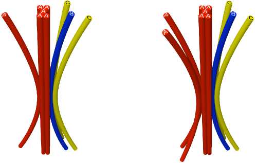
(a)                                              (b)

Figure 1: Schematic images of coinciding 7-branes corresponding to homogeneous Kähler manifolds: (a) $E_{7}/(SU(5)\times U(1)^{3})$ (b) $E_{8}/(SU(5)\times U(1)^{4})$.

The matter curve corresponding to the homogeneous Kähler manifold $E_{8}/(SU(5)\times U(1)^{4})$ is represented by the Weierstrass equation (41) with

$$f(z,w) = -3z^{4}+\alpha z^{3}+\left(a\epsilon-3b^{2}\right)z^{2}+6b\epsilon^{2}z-3\epsilon^{4},$$ (44)

$$g(z,w) = 2z^{6}+z^{5}+\left(b\alpha+\frac{a^{2}}{12}+3\epsilon^{2}\right)z^{4}+(-\epsilon^{2}\alpha-2b^{3}$$ (45)

$$+a\epsilon b)z^{3}+\left(6b^{2}\epsilon^{2}-a\epsilon^{3}\right)z^{2}-6b\epsilon^{4}z+2\epsilon^{6}.$$

The only differences from the curve with (42) and (43) are that it depends on an additional holomorphic parameter $\alpha=\alpha(w)$ satisfying $\alpha(0)=0$, and that $g(z,w)$ (45) contains a $z^{5}$ term. Due to the presence of these terms, the discriminant at $w=0$ reads $\Delta=27z^{10}+108z^{11}$, showing that there are ten 7-branes meeting there to exhibit an $E_{8}$ singularity. The brane configuration is illustrated in FIG. I (b). In this case, compared to the $E_{7}$ case, the string junctions that have an end on the extra A brane yield the massless states listed in TABLE II. The explicit forms of the string junctions can be found in Mizoguchi (2014).

V Conclusions and discussion

In this Letter we have considered a geometric realization of the idea of Sato and Yanagida for explaining the large lepton-flavor mixings and hierarchical Yukawa structures in local F-theory. We have generalized the F-theoretic realization of $E_{7}/(SU(5)\times U(1)^{3})$ obtained in Mizoguchi (2014) to $E_{8}/(SU(5)\times U(1)^{4})$, which naturally gives rise to not only three sets of charged matter fields with family non-universality but the necessary Froggatt-Nielsen fields from the string junctions ending on the extra coinciding 7-brane. Although this mechanism alone does not ensure the existence of three chiral generations in four dimensions, a further compactification and chiral projection, which may be implemented by taking an orbifold or turning on G-fluxes, will lead to a four-dimensional ${\cal N}=1$ $SU(5)$ GUT. If this is done, then we will have an “all-in-one” geometric mechanism in which both the origins of the three families and their large/small mixings can be explained in a single setting. Moreover, the singlet scalars are charged under anomalous $U(1)$s and an FI term will be generated, leading to their acquiring nonzero vevs and triggering SUSY breaking DvaliPomarol ; BinetruyDudas and other effects (see e.g. KNTY ).

Though interesting, however, the following issues must be explored in order for this model to be considered as a realistic model: (i) How the $SU(5)$ anomaly cancels (ii) How the FN fields get the sizes of vevs (14) (iii) How it can be embedded in a global Calabi-Yau and how the neutral moduli are stabilized (iv) How such a brane collision comes into being dynamically. Possible solutions for some of these issues have been suggested in Mizoguchi (2014). As for (i), a possible origin of an extra ${\bf\bar{5}}$ to compensate the anomaly YanagidaYasui is one emerging from the orbifold fixed points since, in the heterotic dual picture (if available), the twisted sector would automatically cure the lack of modular invariance, which is believed to be equivalent to gauge invariance (see e.g. BSS ). We hope to report on these issues elsewhere.

The author thanks T. Kobayashi and Y. Yasui for useful discussions. This work is supported by Grant-in-Aid for Scientific Research (C) #25400285 and (A) #26247042 from The Ministry of Education, Culture, Sports, Science and Technology of Japan.

References

• (1) T. Kugo and T. Yanagida, Phys. Lett. B 134, 313 (1984).
• Mizoguchi (2014) S. Mizoguchi, F-theory Family Unification, arXiv: 1403. 7066 [hep-th]. To appear in JHEP.
• Tani (2001) T. Tani T. Tani, Nucl. Phys. B 602, 434 (2001).
• (4) M. Cvetic, I. Garcia Etxebarria and J. Halverson, JHEP 1111, 101 (2011) [arXiv:1107.2388 [hep-th]].
• (5) M. Dine, N. Seiberg and E. Witten, Nucl. Phys. B 289, 589 (1987).
• (6) J. J. Heckman, A. Tavanfar and C. Vafa, JHEP 1008, 040 (2010) [arXiv:0906.0581 [hep-th]].
• (7) J. Marsano, N. Saulina and S. Schafer-Nameki, JHEP 0908, 046 (2009) [arXiv:0906.4672 [hep-th]].
• (8) E. Dudas and E. Palti, JHEP 1001, 127 (2010) [arXiv:0912.0853 [hep-th]].
• (9) J. Sato and T. Yanagida, Phys. Lett. B 430, 127 (1998) [hep-ph/9710516].
• (10) S. Mizoguchi and M. Yata, PTEP 2013, no. 5, 053B01 (2013) [arXiv:1211.6135 [hep-th]].
• (11) H. Freudenthal, Proc. Kon. Ned. Akad. Wet. A56 (Indagationes Math. 15) (1953) 95-98 (French).
• (12) S. Mizoguchi, Nucl. Phys. B 528, 238 (1998) [hep-th/9703160].
• (13) S. Mizoguchi and G. Schroder, Class. Quant. Grav.  17, 835 (2000) [hep-th/9909150].
• (14) R. Donagi and M. Wijnholt, Adv. Theor. Math. Phys.  15, 1237 (2011) [arXiv:0802.2969 [hep-th]].
• (15) K. Itoh, T. Kugo and H. Kunitomo, ian Coset Space G/h,” Nucl. Phys. B 263, 295 (1986); ian Coset Spaces G/h: G = E6, E7 And E8,” Prog. Theor. Phys.  75, 386 (1986).
• (16) M. Bando, T. Kuramoto, T. Maskawa and S. Uehara, Phys. Lett. B 138, 94 (1984); Prog. Theor. Phys.  72, 313 (1984); Prog. Theor. Phys.  72, 1207 (1984).
• (17) C. D. Froggatt and H. B. Nielsen, Nucl. Phys. B 147, 277 (1979).
• (18) D. R. Morrison and C. Vafa, Nucl. Phys. B 473, 74 (1996) [hep-th/9602114]; Nucl. Phys. B 476, 437 (1996) [hep-th/9603161].
• (19) M. Bershadsky, K. A. Intriligator, S. Kachru, D. R. Morrison, V. Sadov and C. Vafa, Nucl. Phys. B 481, 215 (1996) [hep-th/9605200].
• (20) Y. Kawamura, Prog. Theor. Phys.  103, 613 (2000) [arXiv:hep-ph/9902423]; Prog. Theor. Phys.  105, 691 (2001) [arXiv:hep-ph/0012352]; Prog. Theor. Phys.  105, 999 (2001) [arXiv:hep-ph/0012125].
• (21) C. -L. Ong, Phys. Rev. D 27, 3044 (1983); Phys. Rev. D 31, 3271 (1985).
• (22) S. Irié and Y. Yasui, Z. Phys. C 29 (1985), 123.
• (23) W. Buchmuller and O. Napoly, Phys. Lett. B 163, 161 (1985).
• (24) T. Yanagida and Y. Yasui, Nucl. Phys. B 269, 575 (1986).
• (25) G. R. Dvali and A. Pomarol, Phys. Rev. Lett.  77, 3728 (1996) [hep-ph/9607383].
• (26) P. Binetruy and E. Dudas, Phys. Lett. B 389, 503 (1996) [hep-th/9607172].
• (27) T. Kobayashi, H. Nakano, H. Terao and K. Yoshioka, Prog. Theor. Phys.  110, 247 (2003) [hep-ph/0211347].
• (28) T. Banks, N. Seiberg and E. Silverstein, Phys. Lett. B 401, 30 (1997) [hep-th/9703052].