An Accelerated Proximal Coordinate Gradient Method and its Application to Regularized Empirical Risk Minimization
Abstract
We consider the problem of minimizing the sum of two convex functions: one is smooth and given by a gradient oracle, and the other is separable over blocks of coordinates and has a simple known structure over each block. We develop an accelerated randomized proximal coordinate gradient (APCG) method for minimizing such convex composite functions. For strongly convex functions, our method achieves faster linear convergence rates than existing randomized proximal coordinate gradient methods. Without strong convexity, our method enjoys accelerated sublinear convergence rates. We show how to apply the APCG method to solve the regularized empirical risk minimization (ERM) problem, and devise efficient implementations that avoid full-dimensional vector operations. For ill-conditioned ERM problems, our method obtains improved convergence rates than the state-of-the-art stochastic dual coordinate ascent (SDCA) method.
1 Introduction
Coordinate descent methods have received extensive attention in recent years due to its potential for solving large-scale optimization problems arising from machine learning and other applications (e.g., [29, 10, 47, 17, 45, 30]). In this paper, we develop an accelerated proximal coordinate gradient (APCG) method for solving problems of the following form:
| (1) |
where and are proper and lower semicontinuous convex functions [34, Section 7]. Moreover, we assume that is differentiable on , and has a block separable structure, i.e.,
| (2) |
where each denotes a sub-vector of with cardinality , and the collection form a partition of the components of . In addition to the capability of modeling nonsmooth terms such as , this model also includes optimization problems with block separable constraints. More specifically, each block constraints , where is a closed convex set, can be modeled by an indicator function defined as if and otherwise.
At each iteration, coordinate descent methods choose one block of coordinates to sufficiently reduce the objective value while keeping other blocks fixed. In order to exploit the known structure of each , a proximal coordinate gradient step can be taken [33]. To be more specific, given the current iterate , we pick a block and solve a block-wise proximal subproblem in the form of
| (3) |
and then set the next iterate as
| (4) |
Here denotes the partial gradient of with respect to , and is the Lipschitz constant of the partial gradient (which will be defined precisely later).
One common approach for choosing such a block is the cyclic scheme. The global and local convergence properties of the cyclic coordinate descent method have been studied in, e.g., [41, 22, 36, 2, 9]. Recently, randomized strategies for choosing the block to update became more popular [38, 15, 26, 33]. In addition to its theoretical benefits (randomized schemes are in general easier to analyze than the cyclic scheme), numerous experiments have demonstrated that randomized coordinate descent methods are very powerful for solving large-scale machine learning problems [6, 10, 38, 40]. Their efficiency can be further improved with parallel and distributed implementations [5, 31, 32, 23, 19]. Randomized block coordinate descent methods have also been proposed and analyzed for solving problems with coupled linear constraints [43, 24] and a class of structured nonconvex optimization problems (e.g., [21, 28]). Coordinate descent methods with more general schemes of choosing the block to update have also been studied; see, e.g., [3, 44, 46].
Inspired by the success of accelerated full gradient methods [25, 1, 42, 27], several recent work extended Nesterov’s acceleration technique to speed up randomized coordinate descent methods. In particular, Nesterov [26] developed an accelerated randomized coordinate gradient method for minimizing unconstrained smooth functions, which corresponds to the case of in (1). Lu and Xiao [20] gave a sharper convergence analysis of Nesterov’s method using a randomized estimate sequence framework, and Lee and Sidford [14] developed extensions using weighted random sampling schemes. Accelerated coordinate gradient methods have also been used to speed up the solution of linear systems [14, 18]. More recently, Fercoq and Richtárik [8] proposed an APPROX (Accelerated, Parallel and PROXimal) coordinate descent method for solving the more general problem (1) and obtained accelerated sublinear convergence rate, but their method cannot exploit the strong convexity of the objective function to obtain accelerated linear rates.
In this paper, we propose a general APCG method that achieves accelerated linear convergence rates when the objective function is strongly convex. Without the strong convexity assumption, our method recovers a special case of the APPROX method [8]. Moreover, we show how to apply the APCG method to solve the regularized empirical risk minimization (ERM) problem, and devise efficient implementations that avoid full-dimensional vector operations. For ill-conditioned ERM problems, our method obtains improved convergence rates than the state-of-the-art stochastic dual coordinate ascent (SDCA) method [40].
1.1 Outline of paper
This paper is organized as follows. The rest of this section introduces some notations and state our main assumptions. In Section 2, we present the general APCG method and our main theorem on its convergence rate. We also give two simplified versions of APCG depending on whether or not the function is strongly convex, and explain how to exploit strong convexity in . Section 3 is devoted to the convergence analysis that proves our main theorem. In Section 4, we derive equivalent implementations of the APCG method that can avoid full-dimensional vector operations.
In Section 5, we apply the APCG method to solve the dual of the regularized ERM problem and give the corresponding complexity results. We also explain how to recover primal solutions to guarantee the same rate of convergence for the primal-dual gap. In addition, we present numerical experiments to demonstrate the performance of the APCG method.
1.2 Notations and assumptions
For any partition of into with , there is an permutation matrix partitioned as , where , such that
For any , the partial gradient of with respect to is defined as
We associate each subspace , for , with the standard Euclidean norm, denoted . We make the following assumptions which are standard in the literature on coordinate descent methods (e.g., [26, 33]).
Assumption 1.
The gradient of function is block-wise Lipschitz continuous with constants , i.e.,
An immediate consequence of Assumption 1 is (see, e.g., [25, Lemma 1.2.3])
| (5) |
For convenience, we define the following weighted norm in the whole space :
| (6) |
Assumption 2.
There exists such that for all and ,
The convexity parameter of with respect to the norm is the largest such that the above inequality holds. Every convex function satisfies Assumption 2 with . If , then the function is called strongly convex.
2 The APCG method
In this section we describe the general APCG method, and its two simplified versions under different assumptions (whether or not the objective function is strong convex). We also present our main theorem on the convergence rates of the APCG method.
We first explain the notations used in our algorithms. The algorithms proceed in iterations, with being the iteration counter. Lower case letters , , represent vectors in the full space , and , and are their values at the th iteration. Each block coordinate is indicated with a subscript, for example, represent the value of the th block of the vector . The Greek letters , , are scalars, and , and represent their values at iteration . For scalars, a superscript represents the power exponent; for example, , denotes the squares of and respectively.
input: and convexity parameter .
initialize: set
and choose .
iterate: repeat for
-
1.
Compute from the equation
(7) and set
(8) -
2.
Compute as
(9) -
3.
Choose uniformly at random and compute
-
4.
Set
(10)
The general APCG method is given as Algorithm 1. At each iteration , the APCG method picks a random coordinate and generates , and . One can observe that and depend on the realization of the random variable
while is independent of and only depends on .
To better understand this method, we make the following observations. For convenience, we define
| (11) |
which is a full-dimensional update version of Step 3. One can observe that is updated as
| (12) |
Notice that from (7), (8), (9) and (10) we have
which together with (12) yields
| (13) |
That is, in Step 4, we only need to update the block coordinates as in (13) and set the rest to be .
We now state an expected-value type of convergence rate for the APCG method.
Theorem 1.
For , our results in Theorem 1 match exactly the convergence rates of the accelerated full gradient method in [25, Section 2.2]. For , our results improve upon the convergence rates of the randomized proximal coordinate gradient method described in (3) and (4). More specifically, if the block index is chosen uniformly at random, then the analysis in [33, 20] states that the convergence rate of (3) and (4) is on the order of
Thus we obtain both accelerated linear rate for strongly convex functions () and accelerated sublinear rate for non-strongly convex functions (). To the best of our knowledge, this is the first time that such an accelerated linear convergence rate is obtained for solving the general class of problems (1) using coordinate descent type of methods.
The proof of Theorem 1 is given in Section 3. Next we give two simplified versions of the APCG method, for the special cases of and , respectively.
2.1 Two special cases
For the strongly convex case with , we can initialize Algorithm 1 with the parameter , which implies and for all . This results in Algorithm 2. As a direct corollary of Theorem 1, Algorithm 2 enjoys an accelerated linear convergence rate:
where is the unique solution of (1) under the strong convexity assumption.
input: and convexity parameter .
initialize: set
and .
iterate: repeat for
and repeat for
-
1.
Compute .
-
2.
Choose uniformly at random and compute
-
3.
Set .
Input: .
Initialize: set
and choose .
Iterate: repeat for
-
1.
Compute
-
2.
Compute .
-
3.
Choose uniformly at random and compute
and set for all .
-
4.
Set
Algorithm 3 shows the simplified version for , which can be applied to problems without strong convexity, or if the convexity parameter is unknown. According to Theorem 1, Algorithm 3 has an accelerated sublinear convergence rate, that is
With the choice of , which implies , Algorithm 3 reduces to the APPROX method [8] with single block update at each iteration (i.e., in their Algorithm 1).
2.2 Exploiting strong convexity in
In this section we consider problem (1) with strongly convex . We assume that and have convexity parameters and , both with respect to the standard Euclidean norm, denoted .
Let and be arbitrarily chosen, and define two functions
One can observe that the gradient of the function is block-wise Lipschitz continuous with constants with respect to the norm . The convexity parameter of with respect to the norm defined in (6) is
| (15) |
In addition, is a block separable convex function which can be expressed as , where
As a result of the above definitions, we see that problem (1) is equivalent to
| (16) |
which can be suitably solved by the APCG method proposed in Section 2 with , and replaced by , and , respectively. The rate of convergence of APCG applied to problem (16) directly follows from Theorem 1, with given in (15) and the norm in (14) replaced by .
3 Convergence analysis
In this section, we prove Theorem 1. First we establish some useful properties of the sequences and generated in Algorithm 1. Then in Section 3.1, we construct a sequence to bound the values of and prove a useful property of the sequence. Finally we finish the proof of Theorem 1 in Section 3.2.
Lemma 1.
Suppose and and and are generated in Algorithm 1. Then there hold:
-
(i)
and are well-defined positive sequences.
-
(ii)
and for all .
-
(iii)
and are non-increasing.
-
(iv)
for all .
-
(v)
With the definition of
(17) we have for all ,
Proof.
Due to (7) and (8), statement (iv) always holds provided that and are well-defined. We now prove statements (i) and (ii) by induction. For convenience, Let
Since and , one can observe that and
These together with continuity of imply that there exists such that , that is, satisfies (7) and is thus well-defined. In addition, by statement (iv) and , one can see . Therefore, statements (i) and (ii) hold for .
Suppose that the statements (i) and (ii) hold for some , that is, , and . Using these relations and (8), one can see that is well-defined and moreover . In addition, we have due to statement (iv) and . Using the fact (see the remark after Assumption 2), and a similar argument as above, we obtain and , which along with continuity of imply that there exists such that , that is, satisfies (7) and is thus well-defined. By statement (iv) and , one can see that . This completes the induction and hence statements (i) and (ii) hold.
Next, we show statement (iii) holds. Indeed, it follows from (8) that
which together with and implies that and hence is non-increasing. Notice from statement (iv) and that . It follows that is also non-increasing.
3.1 Construction and properties of
Motivated by [8], we give an explicit expression of as a convex combination of the vectors , and use the coefficients to construct a sequence to bound .
Lemma 2.
Let the sequences , , and be generated by Algorithm 1. Then each is a convex combination of . More specifically, for all ,
| (18) |
where the constants are nonnegative and sum to . Moreover, these constants can be obtained recursively by setting , , and for ,
| (19) |
Proof.
We prove the statements by induction. First, notice that . Using this relation and (9), we see that . From (10) and , we obtain
| (20) | |||||
Since (Lemma 1 (ii)), the vector is a convex combination of and with the coefficients , . For , substituting (9) into (10) yields
Substituting (20) into the above equality, and using from (7), we get
| (21) |
From the definition of in the above equation, we observe that
From the above expression, and using the facts , , and (Lemma 1), we conclude that . Also considering the definitions of and in (21), we conclude that for . In addition, one can observe from (9), (10) and (20) that is an affine combination of and , is an affine combination of and , and is an affine combination of , and . It is known that substituting one affine combination into another yields a new affine combination. Hence, the combination given in (21) must be affine, which together with for implies that it is also a convex combination.
Now suppose the recursion (19) holds for some . Substituting (9) into (10), we obtain that
Further, substituting (the induction hypothesis) into the above equation gives
| (22) | |||||
This gives the form of (18) and (19). In addition, by the induction hypothesis, is an affine combination of . Also, notice from (9) and (10) that is an affine combination of and , and is an affine combination of , and . Using these facts and a similar argument as for , it follows that the combination (22) must be affine.
Finally, we claim for all . Indeed, we know from Lemma 1 that , , . Also, due to the induction hypothesis. It follows that for all . It remains to show that . To this end, we again use (7) to obtain , and use (19) and a similar argument as for to rewrite as
Together with , , and , this implies that . Therefore, is a convex combination of with the coefficients given in (19). ∎
In the following lemma, we construct the sequence and prove a recursive inequality.
Lemma 3.
Let denotes the convex combination of using the same coefficients given in Lemma 2, i.e.,
Then for all , we have and
| (23) |
Proof.
The first result follows directly from convexity of . We now prove (23). First we deal with the case . Using (12), (19), and the facts and , we get
For , we use (12) and the definition of in (8) to obtain that
| (24) | |||||
Using (8) and (9), one can observe that
It follows from the above equation and convexity of that
which together with (24) yields
| (25) |
In addition, from the definition of and , we have
| (26) |
Next, using the definition of and (19), we obtain
| (27) | |||||
Plugging (25) and (26) into (27) yields
where the second inequality is due to . Notice that the right hand side of (25) is an affine combination of , and , and the right hand side of (27) is an affine combination of . In addition, all operations in (3.1) and (3.1) preserves the affine combination property. Using these facts, one can observe that the right hand side of (3.1) is also an affine combination of , and , namely, , where and are defined above.
3.2 Proof of Theorem 1
We are now ready to present a proof for Theorem 1. We note that the proof in this subsection can also be recast into the framework of randomized estimate sequence developed in [20, 14], but here we give a straightforward proof without using that machinery.
Dividing both sides of (7) by gives
| (31) |
Observe from (9) that
| (32) |
It follow from (10) and (31) that
which together with (31), (32) and (Lemma 1 (iv)) gives
Using this relation, (13) and Assumption 1, we have
Taking expectation on both sides of the above inequality with respect to , and noticing that , we get
| (33) | |||||
where the second inequality follows from convexity of .
In addition, by (8), (32) and (Lemma 1 (iv)), we have
| (34) | |||||
where the first equality used (32), the third one is due to (7) and (8), and . This equation together with (33) yields
Using Lemma 3, we have
Combining the above two inequalities, one can obtain that
| (35) |
where
Comparing with the definition of in (11), we see that
| (36) |
Notice that has convexity parameter with respect to . By the optimality condition of (36), we have that for any ,
Using the above inequality and the definition of , we obtain
Now using the assumption that has convexity parameter with respect to , we have
Combining this inequality with (35), one see that
In addition, it follows from (8) and convexity of that
| (38) |
Using this relation and (12), we observe that
where the inequality follows from (38). Summing up this inequality and (3.2) gives
Taking expectation on both sides with respect to yields
which together with , and gives
The conclusion of Theorem 1 immediately follows from , Lemma 1 (v), the arbitrariness of and the definition of .
4 Efficient implementation
The APCG methods we presented in Section 2 all need to perform full-dimensional vector operations at each iteration. In particular, is updated as a convex combination of and , and this can be very costly since in general they are dense vectors in . Moreover, in the strongly convex case (Algorithms 1 and 2), all blocks of also need to be updated at each iteration, although only the th block needs to compute the partial gradient and perform an proximal mapping of . These full-dimensional vector updates cost operations per iteration and may cause the overall computational cost of APCG to be comparable or even higher than the full gradient methods (see discussions in [26]).
In order to avoid full-dimensional vector operations, Lee and Sidford [14] proposed a change of variables scheme for accelerated coordinated gradient methods for unconstrained smooth minimization. Fercoq and Richtárik [8] devised a similar scheme for efficient implementation in the non-strongly convex case () for composite minimization. Here we show that full vector operations can also be avoided in the strongly convex case for minimizing composite functions. For simplicity, we only present an efficient implementation of the simplified APCG method with (Algorithm 2), which is given as Algorithm 4.
input: and convexity parameter .
initialize:
set and ,
and initialize and .
iterate: repeat for
-
1.
Choose uniformly at random and compute
-
2.
Let and , and update
(39)
output:
Proposition 1.
Proof.
We prove by induction. Notice that Algorithm 2 is initialized with , and its first step implies ; Algorithm 4 is initialized with and . Therefore we have
which means that (40) holds for . Now suppose that it holds for some , then
| (41) | |||||
So in Algorithm 4 can be written as
Comparing with (11), and using , we obtain
In terms of the full dimensional vectors, using (12) and (41), we have
Using Step 3 of Algorithm 2, we get
where the last step used (12). Now using the induction hypothesis , we have
Finally,
We just showed that (40) also holds for . This finishes the induction. ∎
We note that in Algorithm 4, only a single block coordinates of the vectors and are updated at each iteration, which cost . However, computing the partial gradient may still cost in general. In Section 5.2, we show how to further exploit problem structure in regularized empirical risk minimization to completely avoid full-dimensional vector operations.
5 Application to regularized empirical risk minimization (ERM)
In this section, we show how to apply the APCG method to solve the regularized ERM problems associated with linear predictors.
Let be vectors in , , …, be a sequence of convex functions defined on , and be a convex function defined on . The goal of regularized ERM with linear predictors is to solve the following (convex) optimization problem:
| (42) |
where is a regularization parameter. For binary classification, given a label for each vector , for , we obtain the linear SVM (support vector machine) problem by setting and . Regularized logistic regression is obtained by setting . This formulation also includes regression problems. For example, ridge regression is obtained by setting and , and we get the Lasso if . Our method can also be extended to cases where each is a matrix, thus covering multiclass classification problems as well (see, e.g., [39]).
For each , let be the convex conjugate of , that is,
The dual of the regularized ERM problem (42), which we call the primal, is to solve the problem (see, e.g., [40])
| (43) |
where . This is equivalent to minimize , that is,
| (44) |
The structure of above matches our general formulation of minimizing composite convex functions in (1) and (2) with
| (45) |
Therefore, we can directly apply the APCG method to solve the problem (44), i.e., to solve the dual of the regularized ERM problem. Here we assume that the proximal mappings of the conjugate functions can be computed efficiently, which is indeed the case for many regularized ERM problems (see, e.g., [40, 39]).
In order to obtain accelerated linear convergence rates, we make the following assumption.
Assumption 3.
Each function is smooth, and the function has unit convexity parameter 1.
Here we slightly abuse the notation by overloading and , which appeared in Sections 2 and 3. In this section represents the (inverse) smoothness parameter of , and denotes the regularization parameter on . Assumption 3 implies that each has strong convexity parameter (with respect to the local Euclidean norm) and is differentiable and has Lipschitz constant 1.
In order to match the condition in Assumption 2, i.e., needs to be strongly convex, we can apply the technique in Section 2.2 to relocate the strong convexity from to . Without loss of generality, we can use the following splitting of the composite function :
| (46) |
Under Assumption 3, the function is smooth and strongly convex and each , for , is still convex. As a result, we have the following complexity guarantee when applying the APCG method to minimize the function .
Theorem 2.
Suppose Assumption 3 holds and for all . In order to obtain an expected dual optimality gap using the APCG method, it suffices to have
| (47) |
where and
| (48) |
Proof.
First, we notice that the function defined in (46) is differentiable. Moreover, for any and ,
where the second inequality used the assumption that has convexity parameter and thus has Lipschitz constant . The coordinate-wise Lipschitz constants as defined in Assumption 1 are
The function has convexity parameter with respect to the Euclidean norm . Let be its convexity parameter with respect to the norm defined in (6). Then
According to Theorem 1, the APCG method converges geometrically:
where the constant is given in (48). Therefore, in order to obtain , it suffices to have the number of iterations to be larger than
This finishes the proof. ∎
Let us compare the result in Theorem 2 with the complexity of solving the dual problem (44) using the accelerated full gradient (AFG) method of Nesterov [27]. Using the splitting in (45) and under Assumption 3, the gradient has Lipschitz constant , where denotes the spectral norm of , and has convexity parameter with respect to . So the condition number of the problem is
Suppose each iteration of the AFG method costs as much as times of the APCG method (as we will see in Section 5.2), then the complexity of the AFG method [27, Theorem 6] measured in terms of number of coordinate gradient steps is
The inequality above is due to . Therefore in the ill-conditioned case (assuming ), the complexity of AFG can be a factor of worse than that of APCG.
Several state-of-the-art algorithms for regularized ERM, including SDCA [40], SAG [35, 37] and SVRG [11, 48], have the iteration complexity
Here the ratio can be interpreted as the condition number of the regularized ERM problem (42) and its dual (43). We note that our result in (47) can be much better for ill-conditioned problems, i.e., when the condition number is much larger than .
Most recently, Shalev-Shwartz and Zhang [39] developed an accelerated SDCA method which achieves the same complexity as our method. Their method is an inner-outer iteration procedure, where the outer loop is a full-dimensional accelerated gradient method in the primal space . At each iteration of the outer loop, the SDCA method [40] is called to solve the dual problem (43) with customized regularization parameter and precision. In contrast, our APCG method is a straightforward single loop coordinate gradient method.
We note that the complexity bound for the aforementioned work are either for the primal optimality (SAG and SVRG) or for the primal-dual gap (SDCA and accelerated SDCA). Our results in Theorem 2 are in terms of the dual optimality . In Section 5.1, we show how to recover primal solutions with the same order of convergence rate. In Section 5.2, we show how to exploit problem structure of regularized ERM to compute the partial gradient , which together with the efficient implementation proposed in Section 4, completely avoid full-dimensional vector operations. The experiments in Section 5.3 illustrate that our method has superior performance in reducing both the primal objective value and the primal-dual gap.
5.1 Recovering the primal solution
Under Assumption 3, the primal problem (42) and dual problem (43) each has a unique solution, say and , respectively. Moreover, we have . With the definition
| (49) |
we have . When applying the APCG method to solve the dual regularized ERM problem, which generate a dual sequence , we can obtain a primal sequence . Here we discuss the relationship between the primal-dual gap and the dual optimality .
Let be a vector in . We consider the saddle-point problem
| (50) |
so that
Given an approximate dual solution (generated by the APCG method), we can find a pair of primal solutions , or more specifically,
| (51) | |||||
| (52) |
As a result, we obtain a subgradient of at , denoted , and
| (53) |
We note that is not only a measure of the dual optimality of , but also a measure of the primal feasibility of . In fact, it can also bound the primal-dual gap, which is the result of the following lemma.
Proof.
The following theorem states that under a stronger assumption than Assumption 3, the primal-dual gap can be bounded directly by the dual optimality gap, hence they share the same order of convergence rate.
Theorem 3.
Suppose is -strongly convex and each is -smooth and also -strongly convex (all with respect to the Euclidean norm ). Given any dual point , let the primal correspondence be , i.e., generated from (52). Then we have
| (54) |
where denotes the spectral norm of .
Proof.
Since is -strongly convex, the function is differentiable and has Lipschitz constant . Similarly, since each is strongly convex, the function is differentiable and has Lipschitz constant . Therefore, the function is smooth and its gradient has Lipschitz constant
It is known that (e.g., [25, Theorem 2.1.5]) if a function is convex and -smooth, then
for all . Applying the above inequality to , we get for all and ,
| (55) |
Under our assumptions, the saddle-point problem (50) has a unique solution , where and are the solutions to the primal and dual problems (42) and (43), respectively. Moreover, they satisfy the optimality conditions
Since is differentiable in this case, we have and . Now we choose and in (55) to be and respectively. This leads to
Then the conclusion can be derived from Lemma 4. ∎
The assumption that each is -smooth and -strongly convex implies that . Therefore the coefficient on the right-hand side of (54) satisfies This is consistent with the fact that for any pair of primal and dual points and , we always have .
Corollary 1.
The above results require that each be both smooth and strongly convex. One example that satisfies such assumptions is ridge regression, where and . For problems that only satisfy Assumption 3, we may add a small strongly convex term to each loss , and obtain that the primal-dual gap (of a slightly perturbed problem) share the same accelerated linear convergence rate as the dual optimality gap. Alternatively, we can obtain the same guarantee with the extra cost of a proximal full gradient step. This is summarized in the following theorem.
Theorem 4.
Proof.
Here the coefficient in the right-hand side of (58), , can be less than . This does not contradict with the fact that the primal-dual gap should be no less than the dual optimality gap, because the primal-dual gap on the left-hand side of (58) is measured at rather than .
Corollary 2.
We note that the computational cost of the proximal full gradient step (56) is comparable with proximal coordinate gradient steps. Therefore the overall complexity of of this scheme is on the same order as necessary for the expected dual optimality gap to reach . Actually the numerical experiments in Section 5.3 show that running the APCG method alone without the final full gradient step is sufficient to reduce the primal-dual gap at a very fast rate.
5.2 Implementation details
Here we show how to exploit the structure of the regularized ERM problem to efficiently compute the coordinate gradient , and totally avoid full-dimensional updates in Algorithm 4.
input: and convexity parameter
.
initialize:
set and ,
and let
, , and .
iterate: repeat for
-
1.
Choose uniformly at random, compute the coordinate gradient
-
2.
Compute coordinate increment
(59) -
3.
Let and , and update
(60)
output: approximate dual and primal solutions
We focus on the special case and show how to compute . In this case, and is the identity map. According to (46),
Notice that we do not form in Algorithm 4. By Proposition 1, we have
So we can store and update the two vectors
and obtain
Since the update of both and at each iteration only involves the single coordinate , we can update and by adding or subtracting a scaled column , as given in (60). The resulting method is detailed in Algorithm 5.
In Algorithm 5, we use to represent to reflect the fact that we never form explicitly. The function in (59) is the one given in (46), i.e.,
Each iteration of Algorithm 5 only involves the two inner products and in computing , and the two vector additions in (60). They all cost rather than . When the ’s are sparse (the case of most large-scale problems), these operations can be carried out very efficiently. Basically, each iteration of Algorithm 5 only cost twice as much as that of SDCA [10, 40].
In Step 3 of Algorithm 5, the division by in updating and may cause numerical problems because as the number of iterations getting large. To fix this issue, we notice that and are always accessed in Algorithm 5 in the forms of and . So we can replace and by
which can be updated without numerical problem. To see this, we have
Similarly, we have
5.3 Numerical experiments
In our experiments, we solve the regularized ERM problem (42) with smoothed hinge loss for binary classification. That is, we pre-multiply each feature vector by its label and let
The conjugate function of is if and otherwise. Therefore we have
For the regularization term, we use . We used three publicly available datasets obtained from [7]. The characteristics of these datasets are summarized in Table 1.
| datasets | source | number of samples | number of features | sparsity |
|---|---|---|---|---|
| RCV1 | [16] | 20,242 | 47,236 | 0.16% |
| covtype | [4] | 581,012 | 54 | 22% |
| News20 | [12, 13] | 19,996 | 1,355,191 | 0.04% |
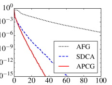
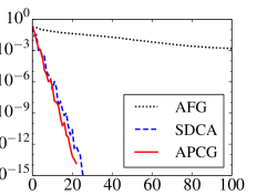
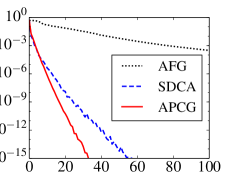
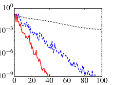
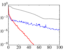
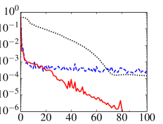
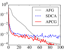
In our experiments, we comparing the APCG method (Algorithm 5) with SDCA [40] and the accelerated full gradient method (AFG) [25] with and additional line search procedure to improve efficiency. When the regularization parameter is not too small (around ), then APCG performs similarly as SDCA as predicted by our complexity results, and they both outperform AFG by a substantial margin.
Figure 1 shows the reduction of primal optimality by the three methods in the ill-conditioned setting, with varying form to . For APCG, the primal points are generated simply as defined in (49). Here we see that APCG has superior performance in reducing the primal objective value compared with SDCA and AFG, even without performing the final proximal full gradient step described in Theorem 4.
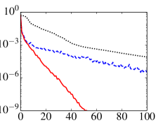
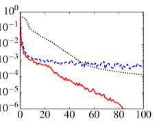
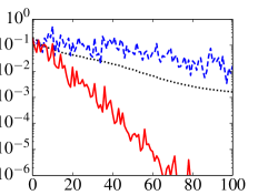
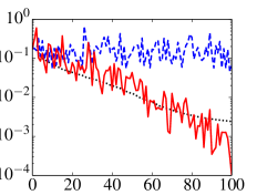
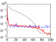
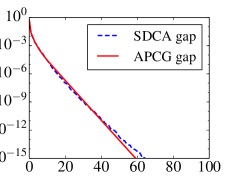
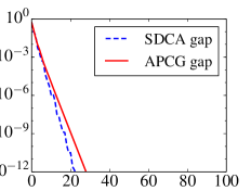
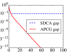
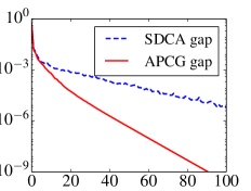
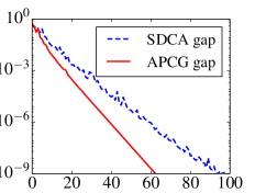
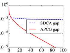
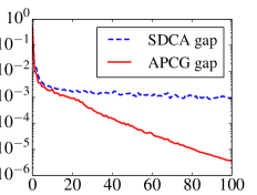
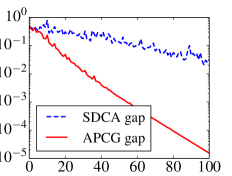
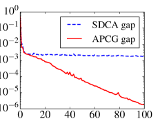
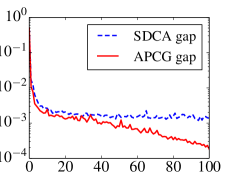
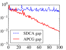
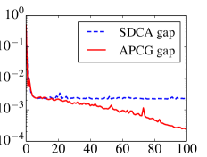
Figure 2 shows the reduction of primal-dual gap by the two methods APCG and SDCA. We can see that in the ill-conditioned setting, the APCG method is more effective in reducing the primal-dual gap as well.
| RCV1 | covertype | News20 | |
|---|---|---|---|
|
 |
 |
|
|
 |
 |
|
|
 |
 |
|
|
 |
 |
| RCV1 | covertype | News20 | |
|---|---|---|---|
|
 |
 |
|
|
 |
 |
|
|
 |
 |
|
|
 |
 |
References
- [1] A. Beck and M. Teboulle. A fast iterative shrinkage-threshold algorithm for linear inverse problems. SIAM Journal on Imaging Sciences, 2(1):183–202, 2009.
- [2] A. Beck and L. Tetruashvili. On the convergence of block coordinate descent type methods. SIAM Journal on Optimization, 13(4):2037–2060, 2013.
- [3] D. P. Bertsekas and J. N. Tsitsiklis. Parallel and Distributed Computation: Numerical Methods. Prentice-Hall, 1989.
- [4] J. A. Blackard, D. J. Dean, and C. W. Anderson. Covertype data set. In K. Bache and M. Lichman, editors, UCI Machine Learning Repository, URL: http://archive.ics.uci.edu/ml, 2013. University of California, Irvine, School of Information and Computer Sciences.
- [5] J. K. Bradley, A. Kyrola, D. Bickson, and C. Guestrin. Parallel coordinate descent for -regularized loss minimization. In Proceedings of the 28th International Conference on Machine Learning (ICML), pages 321–328, 2011.
- [6] K.-W. Chang, C.-J. Hsieh, and C.-J. Lin. Coordinate descent method for large-scale -loss linear support vector machines. Journal of Machine Learning Research, 9:1369–1398, 2008.
- [7] R.-E. Fan and C.-J. Lin. LIBSVM data: Classification, regression and multi-label. URL: http://www.csie.ntu.edu.tw/~cjlin/libsvmtools/datasets, 2011.
- [8] O. Fercoq and P. Richtárik. Accelerated, parallel and proximal coordinate descent. Manuscript, arXiv:1312.5799.
- [9] M. Hong, X. Wang, M. Razaviyayn, and Z. Q. Luo. Iteration complexity analysis of block coordinate descent methods. arXiv:1310.6957.
- [10] C.-J. Hsieh, K.-W. Chang, C.-J. Lin, S. S. Keerthi, and S. Sundararajan. A dual coordinate descent method for large-scale linear svm. In Proceedings of the 25th International Conference on Machine Learning (ICML), pages 408–415, 2008.
- [11] R. Johnson and T. Zhang. Accelerating stochastic gradient descent using predictive variance reduction. In Advances in Neural Information Processing Systems 26, pages 315–323. 2013.
- [12] S. S. Keerthi and D. DeCoste. A modified finite Newton method for fast solution of large scale linear svms. Journal of Machine Learning Research, 6:341–361, 2005.
- [13] K. Lang. Newsweeder: Learning to filter netnews. In Proceedings of the Twelfth International Conference on Machine Learning (ICML), pages 331–339, 1995.
- [14] Y. T. Lee and A. Sidford. Efficient accelerated coordinate descent methods and faster algorithms for solving linear systems. arXiv:1305.1922.
- [15] D. Leventhal and A. S. Lewis. Randomized methods for linear constraints: convergence rates and conditioning. Mathematics of Operations Research, 35(3):641–654, 2010.
- [16] D. D. Lewis, Y. Yang, T. Rose, and F. Li. RCV1: A new benchmark collection for text categorization research. Journal of Machine Learning Research, 5:361–397, 2004.
- [17] Y. Li and S. Osher. Coordinate descent optimization for minimization with application to compressed sensing: a greedy algorithm. Inverse Problems and Imaging, 3:487–503, 2009.
- [18] J. Liu and S. J. Wright. An accelerated randomized Kacamarz algorithm. arXiv:1310.2887, 2013.
- [19] J. Liu, S. J. Wright, C. Ré, V. Bittorf, and S. Sridhar. An asynchronous parallel stochastic coordinate descent algorithm. JMLR W&CP, 32(1):469–477, 2014.
- [20] Z. Lu and L. Xiao. On the complexity analysis of randomized block-coordinate descent methods. Technical Report MSR-TR-2013-53, Microsoft Research, 2013.
- [21] Z. Lu and L. Xiao. Randomized block coordinate non-monotone gradient method for a class of nonlinear programming. arXiv:1306.5918, 2013.
- [22] Z. Q. Luo and P. Tseng. On the convergence of the coordinate descent method for convex differentiable minimization. Journal of Optimization Theory and Applications, 72(1):7–35, 2002.
- [23] I. Necoara and D. Clipici. Distributed random coordinate descent method for composite minimization. Technical Report 1-41, University Politehnica Bucharest, November 2013.
- [24] I. Necoara and A. Patrascu. A random coordinate descent algorithm for optimization problems with composite objective function and linear coupled constraints. Computational Optimization and Applications, 57(2):307–377, 2014.
- [25] Y. Nesterov. Introductory Lectures on Convex Optimization: A Basic Course. Kluwer, Boston, 2004.
- [26] Y. Nesterov. Efficiency of coordinate descent methods on huge-scale optimization problems. SIAM Journal on Optimization, 22(2):341–362, 2012.
- [27] Yu. Nesterov. Gradient methods for minimizing composite functions. Mathematical Programming, Ser. B, 140:125–161, 2013.
- [28] A. Patrascu and I. Necoara. Efficient random coordinate descent algorithms for large-scale structured nonconvex optimization. To appear in Journal of Global Optimization. arXiv:1305.4027, 2013.
- [29] J. Platt. Fast training of support vector machine using sequential minimal optimization. In B. Schölkopf, C. Burges, and A. Smola, editors, Advances in Kernel Methods — Support Vector Learning, pages 185–208. MIT Press, Cambridge, MA, USA, 1999.
- [30] Z. Qin, K. Scheinberg, and D. Goldfarb. Efficient block-coordinate descent algorithms for the Group Lasso. Mathematical Programming Computation, 5(2):143–169, 2013.
- [31] P. Richtárik and M. Takáč. Parallel coordinate descent methods for big data optimization. arXiv:1212.0873, 2012.
- [32] P. Richtárik and M. Takáč. Distributed coordinate descent method for learning with big data. arXiv:1310.2059, 2013.
- [33] P. Richtárik and M. Takáč. Iteration complexity of randomized block-coordinate descent methods for minimizing a composite function. Mathematical Programming, 144(1):1–38, 2014.
- [34] R. T. Rockafellar. Convex Analysis. Princeton University Press, 1970.
- [35] N. Le Roux, M. Schmidt, and F. Bach. A stochastic gradient method with an exponential convergence rate for finite training sets. In Advances in Neural Information Processing Systems 25, pages 2672–2680. 2012.
- [36] A. Saha and A. Tewari. On the non-asymptotic convergence of cyclic coordinate descent methods. SIAM Jorunal on Optimization, 23:576–601, 2013.
- [37] M. Schmidt, N. Le Roux, and F. Bach. Minimizing finite sums with the stochastic average gradient. Technical Report HAL 00860051, INRIA, Paris, France, 2013.
- [38] S. Shalev-Shwartz and A. Tewari. Stochastic methods for regularized loss minimization. In Proceedings of the 26th International Conference on Machine Learning (ICML), pages 929–936, Montreal, Canada, 2009.
- [39] S. Shalev-Shwartz and T. Zhang. Accelerated proximal stochastic dual coordinate ascent for regularized loss minimization. arXiv:1309.2375.
- [40] S. Shalev-Shwartz and T. Zhang. Stochastic dual coordinate ascent methods for regularized loss minimization. Journal of Machine Learning Research, 14:567–599, 2013.
- [41] P. Tseng. Convergence of a block coordinate descent method for nondifferentiable minimization. Journal of Optimization Theory and Applications, 140:513–535, 2001.
- [42] P. Tseng. On accelerated proximal gradient methods for convex-concave optimization. Unpublished manuscript, 2008.
- [43] P. Tseng and S. Yun. Block-coordinate gradient descent method for linearly constrained nonsmooth separable optimization. Journal of Optimization Theory and Applications, 140:513–535, 2009.
- [44] P. Tseng and S. Yun. A coordinate gradient descent method for nonsmooth separable minimization. Mathematical Programming, 117:387–423, 2009.
- [45] Z. Wen, D. Goldfarb, and K. Scheinberg. Block coordinate descent methods for semidefinite programming. In M. F. Anjos and J. B. Lasserre, editors, Handbook on Semidefinite, Cone and Polynomial Optimization: Theory, Algorithms, Software and Applications, volume 166, pages 533–564. Springer, 2012.
- [46] S. J. Wright. Accelerated block-coordinate relaxation for regularized optimization. SIAM Journal on Optimization, 22:159–186, 2012.
- [47] T. Wu and K. Lange. Coordinate descent algorithms for Lasso penalized regression. The Annals of Applied Statistics, 2(1):224–244, 2008.
- [48] L. Xiao and T. Zhang. A proximal stochastic gradient method with progressive variance reduction. arXiv:1403.4699.