Combining cosmological constraints from cluster counts and galaxy clustering
Abstract
Present and future large scale surveys offer promising probes of cosmology. For example the Dark Energy Survey (DES) is forecast to detect 300 millions galaxies and thousands clusters up to redshift 1.3. I here show ongoing work to combine two probes of large scale structure : cluster number counts and galaxy 2-point function (in real or harmonic space). The halo model (coupled to a Halo Occupation Distribution) can be used to model the cross-covariance between these probes, and I introduce a diagrammatic method to compute easily the different terms involved. Furthermore, I compute the joint non-Gaussian likelihood, using the Gram-Charlier series. Then I show how to extend the methods of Bayesian hyperparameters to Poissonian distributions, in a first step to include them in this joint likelihood.
1 Cross-covariance between cluster counts and galaxy clustering
1.1 Cluster counts and galaxy angular 2-point function
The number counts in a bin of mass and redshift , can be considered as a monopole of the halo density field :
| (1) |
Cluster counts have been shown as a powerful probe of cosmology, e.g. [Planck Collaboration XX (2014)] has produced constraint on and with SZ detected clusters.
The study of the clustering of galaxies may be done with the angular correlation function or its harmonic transform , in tomographic redshift bins :
| (2) |
In the following I use instead of for simpler equations, although they can be related by a simple linear transformation.
1.2 Cross-covariance derivation with the halo model
The cross covariance between these two probes involves the halo-galaxy-galaxy angular bispectrum in the squeezed limit [(Lacasa & Rosenfeld, in prep.)] :
| (3) |
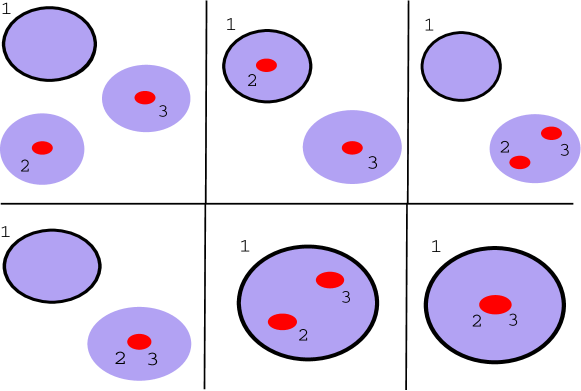
is a projection of the 3D bispectrum, for which we need a non-linear model. In the framework of the halo model + HOD, I have shown that the bispectrum (or higher orders) can be computed with a diagrammatic formalism [(Lacasa et al., 2014)]. See the diagrams for this hgg bispectrum in Fig. 1.
1.3 Current results
I have shown that the equations for the covariance can be rewritten in terms of effective quantities, e.g. [(Lacasa & Rosenfeld, in prep.)] :
| (4) |
These intermediate quantities are integrated over the halo mass and contain the HOD and mass function dependency. They can be compared to measurement on data or to other modeling, providing the possibility for some model independence.
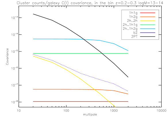
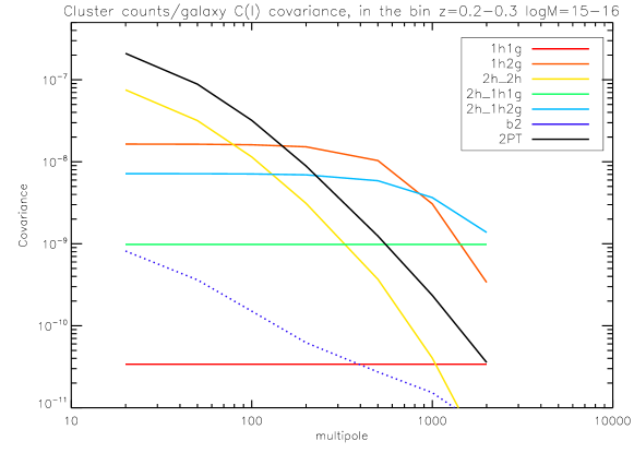
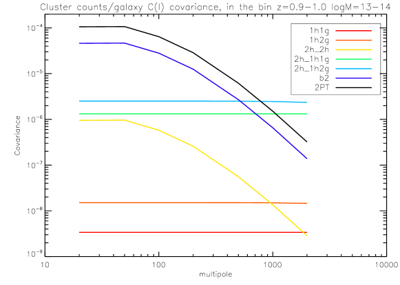
I have built a fast and efficient code to compute the different terms of the covariance ; the plots in Fig. 3 illustrate the numerical results. We see that different terms can become important depending on mass and redshift. The code runs in CPU-second, and is thus adequate to be integrated into an MCMC pipeline.
2 Likelihood
2.1 Joint non-Gaussian likelihood
Cluster counts follow a Poissonian distribution (up to sample variance), thus one cannot assume that the joint likelihood of is Gaussian.
To tackle this, I expanded the joint likelihood with the Gram-Charlier series, around a fiducial independent case. I am then able to resum the expansion into [(Lacasa & Rosenfeld, in prep.)] :
| (5) |
This analytic form is well-behaved (positive), can be extended straightforwardly to include sample variance, and has correct asymptotic behaviour at large (Gaussian with the correct covariance matrix).
2.2 Bayesian hyperparameters
Hyperparameters (HPs) allow to detect over/underestimation of error bars, or inconsistencies between data sets [(see e.g. Hobson et al. 2002)].
The method is at the moment only adapted to Gaussian distributions, thus not for Poissonian cluster counts.
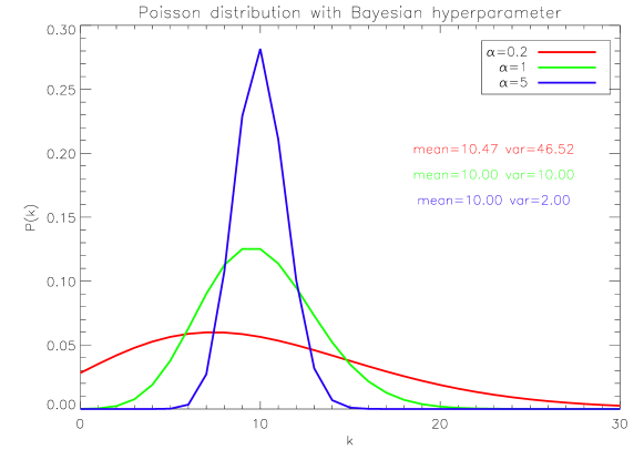
It is however mathematically impossible to keep the Gaussian properties of HPs in the Poissonian case (that is, rescaling the variance while keeping the mean). However I found a prescription which approximately respect them. On Fig. 2 are shown three pdfs, corresponding to three different values of the Bayesian HP .
This will allow the use of HPs for the cluster counts - galaxy 2-pt combination, after further extension (sample variance, correlation with as treated in Sect. 2.1).
3 Conclusion and perspectives
I sketched how to combine cluster counts and galaxy 2-pt measurements for increased cosmological constraints, from the physical modeling to the likelihood. In the context of the halo model, I introduced a diagrammatic method allowing elegant computation of the equations involved. I derived a non-Gaussian joint likelihood using Gram-Charlier series, and showed how to introduce Bayesian HPs to a Poissonian distribution.
Further work will be necessary to include experimental effects in the covariance and the likelihood : photo-z errors, purity… Next order derivation of the joint likelihood may also be necessary to solve a small bias issue at low , and the bayesian hyperparameters method need to be extended to cluster sample variance and correlation with galaxies. In the medium term, I aim to build a full MCMC pipeline of cluster-galaxy combination, for realistic forecasts and application to DES data.
Further details on the model, method, and forecasts will be available in Lacasa & Rosenfeld (in prep.)
4 Figures
References
- [Planck Collaboration XX (2014)] Planck Collaboration (2014), “Planck 2013 results. XX. Cosmology from Sunyaev-Zeldovich cluster counts”, arXiv:1303.5080
- [(Lacasa & Rosenfeld, in prep.)] F. Lacasa and R. Rosenfeld, “Combining cluster counts and galaxy clustering cosmological constraints”, in prep.
- [(Lacasa et al., 2014)] F. Lacasa et al. (2014), “Non-Gaussianity of the CIB anisotropies - I. Diagrammatic formalism and application to the angular bispectrum”, MNRAS, Vol 439, p.123-142
- [(see e.g. Hobson et al. 2002)] M.P. Hobson et al., “Combining cosmological data sets: hyperparameters and Bayesian evidence”, MNRAS, Vol 335, pp. 377-388