A density-functional theory investigation of cluster formation in an effective-potential model of dendrimers

Abstract

We consider a system of particles interacting via a purely repulsive, soft-core potential recently introduced to model effective pair interactions between dendrimers, which is expected to lead to the formation of crystals with multiple occupancy of the lattice sites. The phase diagram is investigated by density-functional theory (DFT) without making any a priori assumption on the functional form of the density profile or on the type of crystal lattice. As the average density $\rho$ is increased, the system displays first a transition from a fluid to a bcc phase, and subsequently to hcp and fcc phases. In the inhomogeneous region, the behavior is that found in previous investigations of this class of cluster-forming potentials. Specifically, the particles arrange into clusters strongly localized at the lattice sites, and the lattice constant depends very weakly on $\rho$, leading to an occupancy number of the sites which is a nearly linear function of $\rho$. These results are compared to those predicted by the more widespread approach, in which the DFT minimization is carried out by representing the density profile by a given functional form depending on few variational parameters. We find that for the model potential studied here, the latter approach recovers most of the predictions of the unconstrained minimization.

I Introduction

Bounded repulsive potentials arise in the description of effective, coarse-grained interactions between polymers. Because of their noncompact nature, mutual overlap between polymers does not require the actual superposition between the constituent monomers and is thus allowed, while still implying a steric repulsion due to the reduction of their available configurations. The prototypical example of these effective soft-core interactions is the repulsive Gaussian two-body potential, whose thorough study stillinger has shown how its equation of state, correlations, and phase diagram differ markedly from those of hard-core fluids.

In recent years, much attention has been given to another class of soft-core repulsive interactions which occur, for instance, in the modelization of ring polymers narros or dendrimers mladekrev2 ; lenz . These interactions differ from the simple Gaussian potential mainly for being softer at small interparticle separation $r$, possibly displaying even a minimum at $r=0$. As a consequence, their Fourier transform is not positive everywhere, and has a negative minimum at non-vanishing wavevector $k_{\rm m}\neq 0$ — a property sometimes referred to as characteristic of the $Q^{\pm}$ class of repulsive interactions likosq , which causes the tendency for the system to self-assemble into regular structures consisting of clusters of particles with a period $\sim 2\pi/k_{\rm m}$, basically independent of density likoschem . This scenario is similar to that giving rise to microphases in hard-core fluids with competing attractive and repulsive interactions compe ; archer , although the physical origin of clustering is different in the two cases. In fluids with competing interactions, clusters occur because on the one hand the attraction favors particle aggregation, while on the other hand the repulsion prevents the aggregates from growing beyond a certain size. In $Q^{\pm}$ repulsive potentials, instead, clustering is due to the fact that particles are allowed to superimpose to each other at the price of a very small mutual repulsion.

The formation of cluster phases in $Q^{\pm}$ potentials has been investigated in detail for the generalized exponential model (GEM) with interaction of the form likoschem ; likosrev :

$$v_{\rm GEM}(r)=\epsilon\exp[-(r/R)^{4}]\,.$$ (1)

In this case one finds that, when the density is increased at sufficiently high temperature, the homogeneous fluid is replaced first by a cluster bcc phase, then by a cluster fcc phase at higher density. Below a triple-point temperature $T_{\rm t}$, the bcc phase disappears, and the only transition left is that between the fluid and the fcc cluster phase likosrev ; mladekrev until, at even lower temperatures, the fcc phase splits into a sequence of fcc phases connected to each other by isostructural transitions, in which the lattice constant jumps discontinuously likosj ; zhang .

Another family of potentials of this class has been proposed as a modelization of the effective interactions between amphiphilic dendrimers with a solvophobic core and a solvophilic shell mladekrev2 ; lenz . In particular, for a specific choice of the parameters which determine the potentials between adjacent and non-adjacent monomers of the dendrimer, the interaction between two isolated dendrimers can be accurately represented by a fit to a sum of two Gaussians of opposite sign lenz :

$$\beta v_{\rm D}(r)=\epsilon_{1}\exp[-(r/R_{1})^{2}]-\epsilon_{2}\exp[-(r/R_{2})^{2}]\,,$$ (2)

where $\beta=1/(k_{\rm B}T)$, $k_{\rm B}$ being the Boltzmann constant, and $\epsilon_{1}=23.6$, $\epsilon_{2}=22.5$, $R_{1}=3.75\sigma$, $R_{2}=3.56\sigma$, $\sigma$ being the diameter of the core monomers. A plot of this potential is displayed in Figure 1. Its Fourier transform $\beta\tilde{v}_{\rm D}(k)$ in the neighborhood of the minimum is shown in the inset.

Figure 1: A plot of the potential $v_{\rm D}(r)$ of Eq. (2) for the interaction between two isolated dendrimers. The inset shows the Fourier transform of the potential $\beta\tilde{v}_{\rm D}(k)$ in the neighborhood of the wave vector $k_{\rm m}$ at which it attains its minimum.

The main qualitative difference between $v_{\rm GEM}(r)$ and $v_{\rm D}(r)$ is that in the latter, $r=0$ corresponds to a minimum rather than a maximum, and the maximum is assumed for $r\neq 0$. This is due to the fact that at small separation between the dendrimers, the overlap between the solvophobic cores contrasts that between the solvophilic shells, thereby leading to a decrease in the repulsion with respect to that felt at intermediate separation when the cores do not overlap, but the shells still do.

Even though the formation of cluster crystals in dendrimers has already been addressed by computer simulation lenz2 , to our knowledge the phase diagram of a system of effective particles interacting by the pair potential (2) has not been considered yet. In the present work, we address this problem by density-functional theory (DFT). We have used a simple, mean-field like free-energy functional, which has already been adopted many times to describe cluster formation in both the soft-core repulsion likoschem ; likosrev ; mladekj and the competing interaction scenario archer . Here, we have given special attention to the procedure followed to minimize the functional. In fact, instead of describing the density profile by a given analytical expression depending on a small number of free parameters, we have not made any a priori hypothesis as to its form save for assuming that it is periodic, and the Bravais lattice vectors which determine the periodicity have themselves been obtained as a result of the minimization. Such a method is computationally more demanding than that more commonly adopted, but its unbiased nature is an asset, since it does not require any guess on the structures into which the system is most likely to assemble.

The plan of the paper is as follows: in Sec. II we briefly introduce the free-energy functional which we have used, and describe the method by which it has been minimized; in Sec. III we apply this method to the study of the phase diagram of a system of dendrimers, described as effective particles interacting via the potential (2); in Sec. IV, we try to get further insight into the results discussed in Sec. III, by assessing up to which extent they can be recovered by adopting an analytical representation of the density profile; finally, in Sec. V we summarize our results and draw our conclusions.

II Theory

In order to study the occurrence and structure of the inhomogeneous phases of a system of particles interacting via the pair potential (2), we have used DFT. According to DFT, at a given temperature $T$, chemical potential $\mu$, and volume $V$, the density profile is obtained by minimizing the grand potential functional $\Omega[\rho({\bf r})]$, whose value then yields the grand potential $-PV$, where $P$ is the pressure. Henceforth, the density profile will be denoted by $\rho({\bf r})$, while $\rho$ with no point-dependence indicated will refer to the average density $\rho\equiv\int\!\!d^{3}{\bf r}\rho({\bf r})/V$. For a system of particles interacting via a pair potential $v({\bf r})$, the exact grand potential functional is of course unknown, and many approximate formulations of DFT have been suggested. Here we have used the following simple form for $\Omega[\rho({\bf r})]$:

$$\beta\Omega=\int\!\!d^{3}{\bf r}\,\rho({\bf r})\!\left\{\ln[\rho({\bf r})\Lambda^{3}]-1-\beta\mu\right\}\,+\,\frac{1}{2}\int\!\!d^{3}{\bf r}\!\!\int\!\!d^{3}{\bf r}^{\prime}\rho({\bf r})\rho({\bf r}^{\prime})\beta v({\bf r}-{\bf r}^{\prime})\,,$$ (3)

where $\Lambda=h/\sqrt{2\pi mk_{\rm B}T}$ is the thermal wavelength of a particle of mass $m$. In the rest of the paper $\Lambda$ will be dropped, since its actual value does not affect any of the results presented here. The first term in the rhs of Eq. (3) is the exact ideal-gas contribution, while the interaction is approximately taken into account in the second, “excess” term. This expression can be considered as a generalization to inhomogeneous systems of the van der Waals mean-field approach, which is in fact obtained from Eq. (3) in the special case of a uniform density profile $\rho({\bf r})\equiv\rho$. A similar approximation for $\Omega[\rho({\bf r})]$ could be adopted also in a system of non-overlapping particles whose pair interaction contains a singular repulsive part, but this would require as a preliminary step to treat separately the singular contribution. Here, instead, $v({\bf r})$ coincides with the total soft-core interaction $v_{\rm D}(r)$ of Eq. (2).

For a homogeneous state, the stability condition with respect to a small perturbation of the density $\delta\rho({\bf r})$

$$\int\!\!d^{3}{\bf r}\!\!\int\!\!d^{3}{\bf r}^{\prime}\!\left.\frac{\delta^{2}(\beta\Omega)}{\delta\rho({\bf r})\delta\rho({\bf r}^{\prime})}\right|_{\rho}\delta\rho({\bf r})\delta\rho({\bf r}^{\prime})>0$$ (4)

is equivalent to the requirement $S(k)>0$ for every wave vector $k$, where $S({\bf k})$ is the structure factor. Equation (3) gives the random-phase approximation (RPA) for $S(k)$:

$$S(k)=[1+\rho\beta\tilde{v}(k)]^{-1}\,,$$ (5)

where $\tilde{v}(k)$ is the Fourier transform of $v(r)$. If $v(r)$ belongs to the $Q^{\pm}$ class, the above condition on $S(k)$ is violated for $\rho>1/[\,\beta|\tilde{v}(k_{\rm m})|\,]$, where $k_{\rm m}$ is the wave vector at which $\tilde{v}(k)$ assumes its negative minimum. The boundary between the region where the homogeneous state is stable and that where it is not corresponds to the condition of marginal stability $\rho=1/[\,\beta|\tilde{v}(k_{\rm m})|\,]$, which identifies a locus in the $T$-$\rho$ plane generally referred to as the $\lambda$-line. Along the $\lambda$-line, the RPA $S(k)$ diverges at $k_{\rm m}$, thus signalling the tendency of the system to form density modulations with a characteristic length $\sim 2\pi/k_{\rm m}$. This can be compared with the behavior on the spinodal line predicted by the RPA for systems which undergo a liquid-vapor transition: in the latter case, the divergence of $S(k)$ occurs for $k=0$, and the homogeneous phase is unstable with respect to separation into two bulk phases.

In the present case in which the potential is athermal, the $\lambda$-line is actually a line at constant $\rho=\rho_{\lambda}$. For the potential (2) one has $k_{\rm m}\sigma=0.941$, $\beta\tilde{v}_{\rm D}(k_{\rm m})/\sigma^{3}=-33.686$, so that $\rho_{\lambda}\sigma^{3}=0.030$. However, it should be recalled that, just like the spinodal line for the liquid-vapor transition, the $\lambda$-line does not generally coincide with the boundary between the homogeneous and the inhomogeneous fluid. The latter must be obtained by comparing the free energies of the two phases, and may (and usually will) lie in a region where the homogeneous fluid is still mechanically stable.

In order to obtain further insight in the phase diagram and the structure of the inhomogeneous phases, it is necessary to turn to the minimization of the functional (3). As stated in Sec. I, we have assumed from the outset that the density profile $\rho({\bf r})$ is periodic, i.e.

$$\rho({\bf r}+{\bf a}_{i})=\rho({\bf r})\,,$$ (6)

where ${\bf a}_{i}$, $i=1$, $2$, $3$, are a set of vectors which define a Bravais lattice. Therefore, $\rho({\bf r})$ can be expanded in a Fourier series:

$$\rho({\bf r})=\frac{1}{v}\sum_{\bf m}e^{-i{\bf k_{m}}\cdot{\bf x}}\,\hat{\rho}_{\bf m}\,,$$ (7)

where $v$ is the volume of the unit cell, ${\bf k_{m}}$ is a vector of the reciprocal lattice, and ${\bf m}$ denotes a set of three indexes $m_{i}=0,\pm 1,\pm 2\ldots$. The expansion coefficients $\hat{\rho}_{\bf m}$ are given by:

$$\hat{\rho}_{\bf m}=\int_{v}\!\!d^{3}{\bf r}\,e^{i{\bf k_{m}}\cdot{\bf r}}\rho({\bf r})\,.$$ (8)

By use of Eqs. (6) and (7), the functional (3) can be rewritten in the following form:

$$\frac{\beta\Omega}{V}=\frac{1}{v}\int_{v}\!\!d^{3}{\bf r}\,\rho({\bf r})\left\{\ln[\rho({\bf r})]-1-\beta\mu\right\}+\frac{1}{2v^{2}}\sum_{\bf m}|\hat{\rho}_{\bf m}|^{2}\,\beta\tilde{v}(\bf k_{m})\,.$$ (9)

We observe that, both in Eq. (8) and (9), the integration in ${\bf r}$ is restricted to the unit cell. Hence, we may set ${\bf r}={\bf A}\cdot{\bf s}$, where ${\bf A}\equiv({\bf a}_{1},{\bf a}_{2},{\bf a}_{3})$ is the matrix obtained by arranging the lattice vectors ${\bf a}_{i}$ into columns, and ${\bf s}$ is a vector whose components vary in the interval $[-1/2,1/2)$. By doing so, it is readily seen that in Eq. (9) neither the ideal-gas term nor the Fourier components of the density profile $\hat{\rho}_{\bf m}$ that appear in the excess term depend on the specific kind of lattice: that is, these quantities are determined solely by the values $\rho({\bf s})\!\equiv\!\rho\,(\!{\bf A}\cdot{\bf s})$ assumed by the density profile in the unit cell, irrespective of the cell geometry. The information on the lattice enters in Eq. (9) only via the reciprocal lattice vectors ${\bf k_{m}}$ at which $\tilde{v}(k)$ is evaluated. This feature makes it easy to implement a numerical procedure, in which the optimization of the grand potential functional (9) is performed with respect to both $\rho({\bf s})$ and the cell geometry, i.e., the elements of ${\bf A}$. In this study, we have assumed that the vectors ${\bf a}_{i}$ of the unit cell are mutually orthogonal, so that ${\bf A}$ is diagonal with eigenvalues $2\pi/h_{i}$, and the reciprocal lattice vectors ${\bf k_{m}}$ have the form ${\bf k_{m}}=(h_{1}m_{1},h_{2}m_{2},h_{3}m_{3})$. This assumption simplifies the calculation, but it could be released without introducing any conceptually new element. To perform the minimization, one has to solve the Euler-Lagrange equations $\delta(\beta\Omega/V)/\delta\rho({\bf r})=0$ as well as $\partial(\beta\Omega/V)/\partial h_{i}=0$, where the functional derivative with respect to $\rho({\bf r})$ and the partial derivative with respect to $h_{i}$ are given by:

$$\frac{\delta}{\delta\rho({\bf r})}\!\left(\frac{\beta\Omega}{V}\right)=\frac{1}{v}\left\{\ln[\rho({\bf r})]-\beta\mu\right\}+\frac{1}{v^{2}}\sum_{\bf m}e^{-i{\bf k_{m}}\cdot{\bf r}}\hat{\rho}_{\bf m}\,\beta\tilde{v}({\bf k_{m}})\,,$$ (10)

$$\frac{\partial}{\partial h_{i}}\!\left(\frac{\beta\Omega}{V}\right)=\frac{1}{v^{2}}\sum_{\bf m}|\hat{\rho}_{\bf m}|^{2}\frac{d\beta\tilde{v}}{d(k^{2})}({\bf k_{m}})\,h_{i}m_{i}^{2}\,.$$ (11)

In the numerical solution, the functional $\Omega[\rho({\bf r})]$ was first discretized by sampling $\rho({\bf r})$ on a finite set of points $\rho_{\bf n}$, so as the replace the functional derivatives with the partial derivatives with respect to $\rho_{\bf n}$. The minimization was then carried out by an iterative algorithm based on the steepest descent. In the basic version of the steepest descent, $\rho_{\bf n}$ and $h_{i}$ are updated recursively by moving “downhill” in the direction opposite to that of the gradient of the discretized functional $\Omega_{\rm D}$:

$$\rho_{\bf n}^{k+1}=\rho_{\bf n}^{k}-\eta\frac{\partial}{\partial\rho_{\bf n}}\!\left.\left(\frac{\beta\Omega_{\rm D}}{V}\right)\right|_{k}\,,$$ (12)

$$h_{i}^{k+1}=h_{i}^{k}-\theta\frac{\partial}{\partial h_{i}}\!\left.\left(\frac{\beta\Omega_{\rm D}}{V}\right)\right|_{k}\,,$$ (13)

where $k$ is the iteration index, and $\eta$, $\theta$ are the parameters which determine the size of the downhill step. In order to increase its efficiency, the above algorithm was improved by introducing preconditioning and conjugate gradients in Eq. (12), and by determining the step-size parameters $\eta$, $\theta$ adaptively at each iteration. A detailed description of these technical features will be given elsewhere gaussmix .

The discretization of the density profile $\rho({\bf r})$ inside the unit cell was performed on $2^{7}\times 2^{7}\times 2^{7}=2\ 097\ 152$ points. The cell in real space was initially chosen as a cube with edge lengh $2\pi/h_{i}=10\sigma$, and was then evolved according to Eq. (13). The trial density profile $\rho_{\rm trial}({\bf r})$ used to start the minimization at a given thermodynamic state was set either to a random noise superimposed to a uniform density, or to a sinusoidal modulation, or to the equilibrium $\rho({\bf r})$ of a nearby state. The need of performing different minimization runs for the same state is due to the fact that soft-core potentials such as that considered here may present many different inhomogeneous structures, each of which corresponds to a local minimum of the grand potential. Hence, the convergence of the algorithm does not guarantee per se that the global minimum has been identified: the search for the latter necessarily involves a comparison between different local minima of the grand potential. Of course, this problem is intrinsic to systems with a complex energy landscape, and many sophisticated strategies have been developed to tackle it genetic ; pickard . However, at the present stage we have not tried to implement any of them, and have just been content with our rather naive approach of performing different runs by changing $\rho_{\rm trial}({\bf r})$.

III Results

By minimizing the grand potential (3) via the algorithm described above it is found that, as expected, the system becomes inhomogeneous at sufficiently high density $\rho$. The phase diagram which we have obtained is shown in Figure 2. Since the potential is athermal, the temperature does not play any role in the phase behavior, which is then determined by the density alone.

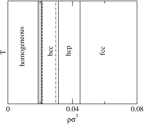
Figure 2: Phase diagram of the potential $v_{\rm D}(r)$ of Eq. (2) obtained by the grand potential functional (3). The gray stripe is the coexistence region between the homogeneous fluid and the bcc phase. The dash-dotted line is the $\lambda$-line (see Sec. II). The dashed line gives the density of the fluid-solid transition according to Eq. (14). The solid lines correspond to the transition between the bcc and hcp phases and to that between the hcp and fcc phases. For both transitions, the coexistence region is too narrow to be resolved on the scale of the figure.

As one moves away from the homogeneous region by increasing $\rho$, the fluid freezes by forming a cluster bcc phase. As anticipated in Sec. II, the $\lambda$-line actually lies inside the inhomogeneous region. The freezing and melting lines have been determined by performing a Maxwell construction, and the corresponding coexistence region is a rather narrow stripe centered at $\rho\sigma^{3}=0.020$. A calculation based on the same free-energy functional used here gives for the density of the fluid-solid transition of $Q^{\pm}$ potentials the expression likoschem :

$$\rho=[\,1.393\beta|\tilde{v}(k_{\rm m})|\,]^{-1}\,.$$ (14)

By substituting the above-mentioned value $\beta\tilde{v}_{\rm D}(k_{\rm m})=-33.686$, this gives $\rho\sigma^{3}=0.021$, in close agreement with the present result.

If $\rho$ is further increased, two more transitions are found, first from the bcc to a hcp phase, then from the hcp to a fcc phase. In both cases the densities of the coexisting phases are very close to each other, so that the width of the coexistence region cannot be resolved on the scale of Figure 2. The transition from a bcc lattice to a close-packed lattice on increasing $\rho$ is in agreement with the general argument put forth in likoschem , as well as with the phase diagram of the GEM potential (1) obtained in likosrev , although in that case the hcp phase was not observed.

The density profile $\rho({\bf r})$ at a density $\rho\sigma^{3}=0.023$ in the bcc region near the fluid-solid boundary is shown in the upper panel of Figure 3 along the direction connecting nearest neighbors as a function of the distance $r$ from a given lattice site.

Figure 3: Open circles: density profile $\rho({\bf r})$ along the direction connecting nearest-neighbor sites for $v_{\rm D}(r)$ at $\rho\sigma^{3}=0.023$ (upper panel) and $v_{\rm GEM}(r)$ at $\rho\sigma^{3}=0.022$ (lower panel) with potential parameters determined as explained in the text. The dashed lines are a guide for the eye. Solid lines: dimensionless potentials $\beta v_{\rm D}(r)$ (upper panel) and $\beta v_{\rm GEM}(r)$ (lower panel) at each lattice site. The lattice is bcc for both potentials.

In order to assess the spatial extension of the density peaks against that of the interaction potential, the latter has also been plotted in the figure. We observe that, despite the proximity to the fluid region, $\rho({\bf r})$ is already strongly localized at the lattice sites. It is interesting to compare this density profile with that of the GEM potential at a similar density. To this purpose, we have considered the interaction (1) at a reduced temperature $k_{\rm B}T/\epsilon=0.8$ such that $\beta v_{\rm GEM}(r=0)=1.25$, somewhere between the well and the hump of $\beta v_{\rm D}(r)$, see Figure 1. The width $R$ of $v_{\rm GEM}(r)$ has then been fixed at the value $R=6.4264\sigma$, for which the integrated intensity of $\beta v_{\rm GEM}(r)$ is the same as that of $\beta v_{\rm D}(r)$. The lower panel of Figure 3 shows $\rho({\bf r})$ obtained by the numerical minimization of the grand potential functional (3) for the GEM potential at $\rho\sigma^{3}=0.022$, as well as $\beta v_{\rm GEM}(r)$ for the parameters given above. The most stable lattice is again the bcc, but the peaks are significantly lower. Since the density is about the same in both panels, this must be compensated by a larger width of the peaks. That this is indeed the case is shown more clearly in Figure 4, where the logarithm of the two density profiles of Figure 3 has been plotted as a function of $r^{2}$.

Figure 4: Open symbols: logarithm of the density profiles displayed in the two panels of Figure 3 for $v_{\rm D}(r)$ (open circles) and $v_{\rm GEM}(r)$ (triangles), as a function of the square of the distance from a given lattice site. Filled symbols: same as the above for $v_{\rm D}(r)$ and $\rho\sigma^{3}=0.046$ (squares), $\rho\sigma^{3}=0.093$ (circles). The dashed lines are a guide for the eye.

Hence, the dendrimer potential $v_{\rm D}(r)$ leads to a higher localization with respect to the GEM potential, and it is natural to trace this back to the minimum of $v_{\rm D}(r)$ at $r=0$. We also note that on the scale of Figure 4, a Gaussian $\rho({\bf r})$ corresponds to a straight line. It appears that, for both $v_{\rm D}(r)$ and $v_{\rm GEM}(r)$, $\rho({\bf r})$ can be accurately represented by a Gaussian as long as one has $\rho({\bf r})\sigma^{3}\lesssim 0.1$, as one would expect from Figure 3. Deviations from the Gaussian profile become evident at smaller $\rho({\bf r})$.

As one moves more deeply into the inhomogeneous region, the height of the peaks of the density profile increases very rapidly, as shown in Figure 5 which displays $\rho({\bf r})$ in the fcc domain for $\rho\sigma^{3}=0.046$ and $\rho\sigma^{3}=0.093$. These $\rho({\bf r})$ have also been plotted in Figure 4 in order to show that the peaks become narrower and narrower on increasing $\rho$.

Figure 5: Same as the upper panel of Figure 3 for $\rho\sigma^{3}=0.046$ (squares) and $\rho\sigma^{3}=0.093$ (circles). The dashed lines are a guide for the eye. The lattice is fcc for both densities.

On the other hand, by comparing Figures 3 and 5 it appears that the nearest-neighbor distance $d$ is hardly affected by density. In fact, this behavior is peculiar of crystals formed by $Q^{\pm}$ potentials for which, even though the specific kind of periodicity of $\rho({\bf r})$ depends of course on the lattice formed by the system, its spatial extent is basically determined only by the density-independent wave vector $k_{\rm m}$ of the minimum of the potential in Fourier space likoschem . At variance with atomic crystals, this leads to a nearest-neighbor distance $d$ and a volume per lattice site $v_{0}$ which are nearly unaffected by $\rho$. Since the number of particles $n_{c}$ in a cluster located at a lattice site is related to the average density $\rho$ by the relation likoschem $\rho=n_{c}/v_{0}$, a nearly constant $v_{0}$ implies a nearly linear dependence of $n_{c}$ on $\rho$.

The nearest-neighbor distance and the number of particles per cluster are shown in Figure 6 for the fcc phase. Although not strictly constant, $d$ is indeed found to be a very slowly varying function of density, giving the anticipated linear dependence of $n_{c}$ on $\rho$. It is interesting to observe that, as $\rho$ is increased, $d$ is actually found to increase, albeit slightly so. At first this may appear at odds with the fact that, if the particle number $N$ is kept constant and $\rho$ is increased, the volume of the system must obviously decrease, but in fact no contradiction arises, since the slight increase in $v_{0}$ is more than compensated by the decrease in the number of lattice sites $N_{l}=N/n_{c}$. In other words, a cluster crystal manages to change its volume not by changing the lattice spacing, but rather the number of lattice sites, and consequently their population $n_{c}$. In this respect, whether $d$ increases or decreases on increasing $\rho$ is of little relevance, provided it remains a slowly varying function of $\rho$.

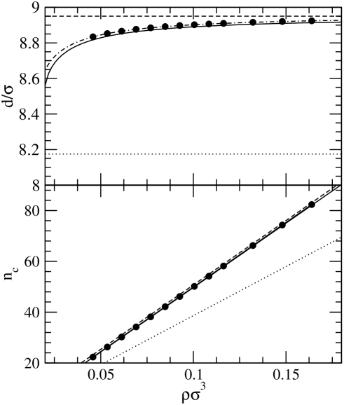
Figure 6: Nearest-neighbor distance $d$ (upper panel) and number of particles in a cluster $n_{c}$ (lower panel) for the potential $v_{\rm D}(r)$ in the fcc phase. The filled circles are the result obtained by the numerical minimization of functional (3). The dotted lines are the result obtained by estimating $d$ from the wave vector $k_{\rm m}$ of the minimum of $\tilde{v}_{\rm D}(k)$. The dashed and solid lines have been obtained by representing the density profile by a superposition of $\delta$-like peaks or Gaussians respectively, and taking into account only onsite and nearest-neighbor interactions. The dot-dashed line in the upper panel has been obtained by the Gaussian representation of the density profile and inclusion of the interactions beyond nearest neighbors, see Sec. IV.

IV Analytical representation of $\rho({\bf r})$

As evident from Figures 3 and 5, as $\rho$ increases the density profile becomes very strongly localized at the lattice sites. It is then natural to represent it by a sum of non-overlapping or weakly overlapping peaks centered at these sites. The crudest approximation of this kind consists in assuming the highest degree of localization, and modeling $\rho({\bf r})$ as a sum of $\delta$-functions:

$$\rho_{\delta}({\bf r})=n_{c}\sum_{\bf m}\delta({\bf r}-{\bf R_{m}})\,,$$ (15)

where ${\bf R_{m}}$ describe the positions of the lattice sites. Strictly speaking, Eq. (15) cannot be true, since it would imply an infinite free energy cost due to the loss of translational entropy. In a system with temperature-independent interactions, Eq. (15) would hold at $T=0$, but then $n_{c}$ could not be chosen at one’s will, since it would be bounded to assume integer values likosj . However, the above assumption still makes sense as an approximation, if one assumes that, for the true $\rho({\bf r})$, the free energy is dominated by its energetic contribution and may thus be approximated by disregarding the entropic term altogether. One is then left with an internal energy per particle $(E/N)_{\delta}$ which, for $\rho({\bf r})$ of Eq. (15), has the form:

$$\left(\frac{\beta E}{N}\right)_{\!\delta}=\frac{1}{2}\zeta d^{3}\!\rho[\,\beta v_{\rm D}(0)+\sum_{m\neq 0}q_{m}\beta v_{\rm D}(c_{m}d)\,]-\frac{1}{2}\beta v_{\rm D}(0)\,.$$ (16)

In the above expression, $v_{\rm D}(0)$ represents the interaction between particles belonging to the same cluster, and the interaction between different clusters is given by the lattice sum of the potential over successive neighbor shells. The constants $q_{m}$ and $c_{m}$ are specific to the lattice considered, and represent respectively the number of $m$-th neighbors and their distance from a given lattice site in units of the nearest-neighbor distance $d$. The number of particles per cluster $n_{c}$ has been expressed as $\zeta d^{3}\rho$, where the quantity $\zeta d^{3}$ is the volume per lattice site $v_{0}$ expressed as a function of $d$, and again $\zeta$ depends on the lattice: in particular, $\zeta\!=\!4\sqrt{3}/9$ for the bcc lattice and $\zeta\!=\!\sqrt{2}/2$ for the fcc and hcp lattices. If Eq. (16) is truncated at the nearest-neighbor level, one obtains:

$$\left(\frac{\beta E}{N}\right)_{\!\delta}\simeq\frac{1}{2}\zeta d^{3}\!\rho\left[\,\beta v_{\rm D}(0)+q\beta v_{\rm D}(d)\,\right]\,,$$ (17)

where $q\equiv q_{1}$ is the number of nearest neighbors. Equation (17) can be regarded as a simple variational expression to be minimized at fixed $\rho$ with respect to the single variational parameter $d$. Again, we must observe that this statement taken at face value makes little sense, since the minimum of Eq. (17) at fixed $\rho$ is actually obtained for $d=0$: in other words, this expression does not prevent the unphysical collapse of the crystal at a single lattice point. What drives the system away from such a collapse is the fact that, as $d$ is decreased, more and more shells contribute significantly to the energy. This leads to a divergence of the sum in Eq. (16), but such an occurrence is lost in Eq. (17), which contains just one shell. Nevertheless, Figures 3 and 5 indicate that, at the actual $d$, the interaction energy between different lattice sites is rapidly decreasing with their distance, so that the contribution due to the outer shells should indeed be very small. Hence, although Eq. (17) cannot be trusted at every $d$, it might still be a reasonable approximation in the neighborhood of the value of $d$ chosen by the system, which would then be recovered as a local minimum of Eq. (17). In fact, besides the spurious minimum at $d=0$, this expression is found to have a (spurious) local maximum and a local minimum. The latter is equal to $d_{\rm bcc}=8.35\sigma$ for the bcc lattice and $d_{\rm fcc}=8.95\sigma$ for the fcc and hcp lattices. In Figure 6 we have reported $d_{\rm fcc}$ together with the value $d_{\lambda}=\pi\sqrt{6}/k_{\rm m}$ obtained by identifying the wave vector $k_{\rm m}$ of the minimum of $\tilde{v}_{\rm D}(k)$ with the nearest-neighbor distance in reciprocal space, which yields $d_{\lambda}=8.17$. One sees that $d_{\rm fcc}$ is a rather accurate estimate of the nearest-neighbor distance, actually more so than $d_{\lambda}$. As a consequence, also the slope of the $n_{c}$ vs. $\rho$ plot is accurately reproduced.

The value of $d$ obtained from the minimization of $(E/N)_{\delta}$ is clearly independent of density, and this would be true even if the summation over all neighbor shells of Eq. (16) were used instead of the truncated expression of Eq. (17). In order to describe the dependence of $d$ on density, the contribution of the translational entropy to the free energy must be taken into account, and this in turn requires to go beyond the representation of $\rho({\bf r})$ as a superposition of $\delta$-like spikes. Following Refs. likosrev and likoschem , we then replace the $\delta$-functions in Eq. (16) with Gaussians of finite amplitude:

$$\rho_{G}({\bf r})=n_{c}\left(\frac{\alpha}{\pi}\right)^{3/2}\sum_{\bf m}e^{-\alpha({\bf r}-{\bf R_{m}})^{2}}\,,$$ (18)

where the normalization constant has been determined so that $n_{c}$ gives the number of particles at each site as requested. If $\rho_{G}({\bf r})$ is substituted into Eq. (3) and the overlap between the Gaussians at different lattice sites is neglected in the ideal-gas term, then the following expression for the Helmholtz free energy $F\equiv\Omega+\mu\int\!d^{3}{\bf r}\rho({\bf r})$ is obtained likosrev :

$$\left(\frac{\beta F}{N}\right)_{\!\rm G}\!=\ln n_{c}+\frac{3}{2}\ln\frac{\alpha}{\pi}-\frac{5}{2}+n_{c}\sqrt{\frac{\alpha^{3}}{2\pi}}\int_{0}^{+\infty}\!\!\!dr\,r^{2}e^{-\alpha r^{2}/2}\,\beta v(r)$$

$$\mbox{}+n_{c}\sqrt{\frac{\alpha}{8\pi}}\sum_{{\bf m}\neq 0}\frac{1}{R_{\bf m}}\int_{0}^{+\infty}\!\!\!dr\,r\left[e^{-\alpha(r-R_{\bf m})^{2}/2}-e^{-\alpha(r+R_{\bf m})^{2}/2}\right]\beta v(r)\,.$$ (19)

For the potential $v_{\rm D}(r)$, the integrals in Eq. (19) can be performed analytically, and one has:

$$\mbox{}\left(\frac{\beta F}{N}\right)_{\!\rm G}\!=\ln(\zeta d^{3}\rho)+\frac{3}{2}\ln\frac{\alpha}{\pi}-\frac{5}{2}+\frac{1}{2}\,\zeta d^{3}\rho\left\{\epsilon_{1}\!\left(\frac{\alpha}{\alpha+\gamma}\right)^{3/2}\!\{1+\sum_{m\neq 0}q_{m}e^{-\alpha\gamma c_{m}^{2}d^{2}/[2(\alpha+\gamma)]}\,\}\right.$$

$$\left.-\epsilon_{2}\!\left(\frac{\alpha}{\alpha+\delta}\right)^{3/2}\!\{1+\sum_{m\neq 0}q_{m}e^{-\alpha\delta c_{m}^{2}d^{2}/[2(\alpha+\delta)]}\,\}\right\}\,,$$ (20)

where $\gamma=2/R_{1}^{2}$, $\delta=2/R_{2}^{2}$, and we have expressed $n_{c}$ as $n_{c}=\zeta d^{3}\rho$ as before. In the limit $\alpha\rightarrow\infty$, the interaction term in Eq. (20) reproduces Eq. (16), save for the thermodynamically irrelevant term $-\beta v_{\rm D}(0)/2$. However, the minimization of the free energy $(\beta F/N)_{\rm G}$ must now be carried out with respect to both $d$ and $\alpha$. This requires the solution of the non-linear system of equations $\partial(\beta F/N)_{\rm G}/\partial d=\partial(\beta F/N)_{\rm G}/\partial\alpha=0$. If we make the change of variables:

$$x = \frac{\gamma d^{2}}{2(1+\gamma/\alpha)}\,,$$

$$y = \frac{\delta d^{2}}{2(1+\delta/\alpha)}\,,$$ (21)

the above system can be cast in the rather symmetric form:

$$x = H\frac{\gamma}{\delta}\,\frac{yS(y)}{HS(y)-3}\,,$$

$$y = K\frac{\delta}{\gamma}\,\frac{xS(x)}{KS(x)+3}\,,$$ (22)

where we have set:

$$H = \sqrt{2}\,\zeta\rho\frac{\epsilon_{2}}{\delta^{3/2}}\,,$$

$$K = \sqrt{2}\,\zeta\rho\frac{\epsilon_{1}}{\gamma^{3/2}}\,,$$ (23)

and the function $S(x)$ is defined by:

$$S(x)=x^{3/2}\left[3+\sum_{m\neq 0}q_{m}(3-2c_{m}^{2}x)e^{-c_{m}^{2}x}\right]\,.$$ (24)

We can now introduce the same approximation used in going from Eq. (16) to Eq. (17) by truncating $S(x)$ at the nearest-neighbor shell:

$$S(x)\simeq x^{3/2}\left[3+q(3-2x)e^{-x}\right]\,.$$ (25)

As observed above for Eq. (17), strictly speaking such a truncation would lead to the collapse of the crystal at $d=0$, but one expects that a physical solution may still be recovered as a local minimum of the free energy thus obtained. The results for $d$ and $n_{c}$ given by the numerical solution of Eq. (22) with the approximation (25) for the fcc lattice are again displayed in Figure 6. Both $d$ and $n_{c}$ run very close to the corresponding quantities obtained from the fully numerical minimization of the free energy described in Sec. II. It appears then that, provided the finite amplitude of the density peaks is taken into account, keeping the interactions only up to nearest neighbors is already sufficient to reproduce accurately the density dependence of $d$, at least at high density where the fcc phase is favored. For the bcc phase, it turns out that also the second-nearest neighbor shell must be included in the calculation. This is due to the fact that in the bcc lattice the nearest and second-nearest neighbor shells are much closer to each other than in the fcc lattice. In either the fcc or the bcc, inclusion of the other neighbor shells from the third on leads to a result which is indistinguishable from that given by the fully numerical calculation, as again shown in the figure for the fcc phase.

In view of such an agreement, it is natural to ask how the phase behavior predicted by Eq. (20) on the basis of the Gaussian parameterization of the density profile (18) compares with that discussed at the beginning of Sec. III. This is a rather subtle issue, because the free energies of the different phases are very close to one another. Therefore, even a small change in their values may alter their relative balance. In fact, it is found that the truncation of the interactions at the nearest-neighbor level in Eq. (20) has rather important consequences on the phase diagram, because it would make the bcc phase more stable than both the fcc and hcp phases even at high density, thus leaving the bcc as the only inhomogeneous phase. In order to recover the stability of the close-packed structures at high density, in Eq. (20) the interactions have to be taken into account at least up to the second-nearest neighbor shell. As recalled above, the contribution of this shell is much more substantial in the bcc lattice than in either the fcc or hcp, and proves crucial in order to move the bcc free energy above that of the close-packed lattices. In Figure 7 we show the free energy per particle $F/N$ and the grand potential per unit volume $\Omega/V$ of the bcc, fcc and hcp phases obtained via the minimization of Eq. (20) by including a rather large number of neighbor shells such that, for the densities considered, the addition of further shells would leave the free energy unchanged within numerical accuracy.

Figure 7: Helmholtz free energy per particle $F/N$ as a function of density in the inhomogeneous region, measured with respect to that of the homogeneous fluid $F_{\rm h}/N$. The symbols refer to the results of the fully numerical minimization for the bcc (circles), fcc (squares), and hcp phases (crosses). The solid line is the result obtained by representing $\rho({\bf r})$ by a superposition of Gaussians, see Eqs. (18) and (20). In both cases, the free energy differences between different phases cannot be resolved on the scale of the figure. Inset: same as the above for the grand potential per unit volume $\Omega/V$ measured with respect to that of the homogeneous fluid $\Omega_{\rm h}/V$.

These results are compared to those given for the same phases by the fully numerical minimization. It is evident that the two sets of data are indistinguishable on the scale of the figure. Moreover, for both sets of data the free energies and grand potentials corresponding to different phases are also indistinguishable, although by enlarging the energy scale the small differences which determine the most stable phase at a certain density would be appreciated. In particular, Eq. (20) predicts that the bcc lattice becomes unfavorite with respect to close-packed lattices for $\rho\sigma^{3}>0.031$, in very good agreement with the position of the bcc-hcp transition shown in Figure 2.

There is, however, a difference between the phase behavior given by the unconstrained minimization discussed in Sec. III and that given by Eq. (20), namely, while the former predicts the occurrence of the hcp phase between the bcc and fcc phases, according to the latter the free energy of the hcp phase is always higher than that of the fcc phase. Hence, the hcp phase is not observed, and as the density is increased the sequence of phase transitions is fluid–bcc–fcc instead of fluid–bcc–hcp–fcc as in Figure 2. Nevertheless, it should be remarked that in both cases the free energies of the hcp and fcc phases are everywhere extremely close to each other: specifically, their relative difference is of the order of $\sim 10^{-6}$, while that between the bcc and fcc phases is $\sim 10^{-3}$. This is not surprising, in the light of the fact that the free energies of the fcc and hcp lattices become distinct only from the third-neighbor shell on. Therefore, even though the numerical accuracy of the calculation is high enough to allow resolution of such tiny differences, speaking of a “most stable” phase in this context is somewhat academic, and one should more realistically regard the fcc and hcp phases as nearly degenerate. One also expects that whether the contributions to the free energy from the high-order shells will stabilize one phase or the other will most likely depend on rather specific features of the decay of the potential at long distance.

V Conclusions

We have employed density-functional theory to study the phase diagram and the density profile of a system of particles interacting via an athermal, penetrable-core potential $v_{\rm D}(r)$ aimed at modeling the effective pair interaction between dendrimers lenz . The potential belongs to the so-called $Q^{\pm}$ class likosq , which is expected to lead to the formation of cluster crystals at high enough density. The results discussed in the paper confirm this prediction, and the main features of the behavior of the system are those already encountered in the study of the generalized exponential model potential $v_{\rm GEM}(r)=\epsilon\exp[-(r/R)^{4}]$ carried out some years ago likoschem ; likosrev . Specifically: i) in the inhomogeneous phases, the particles arrange into clusters localized at the lattice sites, such that each cluster contains many particles. ii) The lattice spacing is nearly independent of density, which in turn implies that the number of particles per cluster is a nearly linear function of density. In the present system the localization is even stronger than that observed in the GEM potential, because of the local minimum presented by $v_{\rm D}(r)$ at $r=0$. iii) As the density is increased, one observes a transition from the bcc structure to close-packed structures. Here we find both hcp and fcc phases, while for the GEM potential the hcp phase was not observed.

The density functional which we have adopted has the same mean-field form already used in the study of the GEM potential likoschem ; likosrev . The minimization of the functional has been performed by a parameter-free procedure, in which both the values assumed by the density profile $\rho({\bf r})$ and the lattice structure were determined as the outcome of the calculation. The only assumptions which we made are that the density profile is periodic, and that the unit cell can be represented by a set of mutually orthogonal vectors. Although not absolutely general, this assumption does not necessarily rule out the occurrence of structures whose primitive cell cannot be represented in this way, e.g. the aforementioned hcp lattice. The results thus obtained have then been compared with those given by the more common procedure, in which one considers a priori a set of possible lattice structures, represents $\rho({\bf r})$ as a superposition of Gaussians centered at the lattice sites, and identifies the most stable structure among the selected ones by inspection of their free energies once the minimization has been carried out. The comparison shows that the Gaussian parameterization reproduces most of the results obtained by the unconstrained minimization. In fact, for the densities at which the system arranges into a close-packed lattice, its properties can be already described very satisfactorily by further simplifying the treatment, and disregarding the contribution to the excess free energy beyond nearest-neighbor lattice sites, although this contribution is necessary in order to account for the transition from the bcc to the fcc structure. The only qualitative prediction which we did not recover by the Gaussian representation of $\rho({\bf r})$ is the occurrence of the hcp phase between the bcc and fcc, the fcc phase being always favored with respect to the hcp. However, in both approaches the relative differences in free energy between the two structures are extremely small, so that labelling either of them as the more stable one is of little practical relevance. In fact, these differences are due to the interactions from the third nearest-neighbor shell on, which we expect to depend on rather specific details of the decay of the interaction at long distance. In the light of these considerations, for the system considered here the unconstrained minimization may admittedly appear as an overkill. One can easily imagine, however, that this may not be the case in other situations, in which the density profile is less amenable to being described by a superposition of Gaussians. We plan to report on such an instance in the near future gaussmix .

Before concluding this discussion, one more consideration is in order: since the potential $v_{\rm D}(r)$ has been introduced as a representation of pair interactions between dendrimers, one may ask whether real dendrimers can be expected to display the behavior described above, especially as far as cluster formation is concerned. This depends on the actual relevance of many-body interactions, which are disregarded in the present picture. The very fact that, according to the density profile predicted on the basis of $v_{\rm D}(r)$, most particles concentrate at the lattice sites leading to very high values of the local density, suggests that many-body effects are indeed relevant, and may significantly influence the behavior of the system. This conclusion was reached in a computer simulation study of an assembly of ring polymers narros . For that system, the pair potential between two isolated polymers displays a profile similar to that of $v_{\rm D}(r)$. In particular, it also belongs to the $Q^{\pm}$ class, so that it is expected to promote cluster formation. However, it was found that at finite density many-body effects lead to an effective pair interaction which is substantially modified with respect to its zero-density limit, to the point that clustering does not take place. In such a situation, the pair interaction between two isolated ring polymers is clearly of little use in understanding the behavior of the system. On the other hand, a subsequent study showed that in dendrimers the formation of cluster crystals does take place lenz2 , although many-body effects are still very important. In fact, they prevent the number of dendrimers per lattice site $n_{c}$ from growing indefinitely, as is instead predicted by the two-body potential, and inhibit the formation of the crystal at high density, where a percolated network of dendrimers is favored. Moreover, in line with this tendency of many-body interactions to curb the growth of $n_{c}$ with $\rho$, the lattice spacing was found to be a slowly decreasing function of $\rho$, rather than a slowly increasing one as in the present study. It should also be observed that the parameters of the interactions between monomers used in lenz2 are different from those used in lenz , and the resulting pair potential for isolated dendrimers leads to clustering at a lower density than that obtained with the pair potential (2) considered here. Nevertheless, it is reassuring to have evidence that for this system the formation of cluster crystals does not rest solely upon the effective pair potential picture.

References

- (1) F. H. Stillinger and D. K. Stillinger, Physica A 244, 358 (1977); A. Lang, C. N. Likos, M. Watzlawek and H. Löwen, J. Phys.: Condens. Matter 12, 5087 (2000); C. N. Likos, Phys. Rep. 348, 267 (2001).
- (2) A. Narros, A. J. Moreno, and C. N. Likos, Soft Matter 6, 2435 (2010).
- (3) B. M. Mladek, G. Kahl, and C. N. Likos, Phys. Rev. Lett. 100, 028301 (2008).
- (4) D. A. Lenz, B. M. Mladek, C. N. Likos, G. Kahl, and R. Blaak, J. Phys. Chem. B 115, 7218 (2011).
- (5) C. N. Likos, A. Lang, M. Watzlawek, and H. Löwen H Phys. Rev. E 63, 031206 (2001).
- (6) C. N. Likos, B. M. Mladek, D. Gottwald, and G. Kahl, J. Chem. Phys. 126, 224502 (2007).
- (7) R. P. Sear, S.-W. Chung, G. Markovich, W. M. Gelabrt, and J. R. Heath, Phys. Rev. E 59, R6255 (1999); R. P. Sear and W. M. Gelbart, J. Chem. Phys. 110, 4582 (1999); A. Imperio and L. Reatto, J. Phys.: Condens. Matter 16, S3769 (2004); A. Imperio and L. Reatto, J. Chem. Phys. 124, 164712 (2006); A. Imperio and L. Reatto, Phys. Rev. E 76, 040402 (2007); A. J. Archer A J and N. B. Wilding, Phys. Rev. E 76, 031501 (2007);
- (8) A. J. Archer, Phys. Rev. E 78, 031402 (2008).
- (9) B. M. Mladek, D. Gottwald, G. Kahl, M. Neumann, and C. N. Likos, Phys. Rev. Lett 96, 045701 (2006).
- (10) B. M. Mladek, P. Charbonneau, and D. Frenkel, Phys. Rev. Lett. 99, 235702 (2007).
- (11) T. Neuhaus and C. N. Likos, J. Phys.: Condens. Matter 23, 234112 (2011).
- (12) K. Zhang, P. Charbonneau, and B. M. Mladek, Phys. Rev. Lett. 105, 245701 (2010); N. B. Wilding and P. Sollich, EPL 101,10004 (2013).
- (13) D. A. Lenz, R. Blaak, C. N. Likos, and B. M. Mladek, Phys. Rev. Lett. 109, 228301 (2012).
- (14) B. M. Mladek, D. Gottwald, G. Kahl, M. Neumann, and C. N. Likos, J. Chem. Phys. B 111, 12799 (2007).
- (15) D. Pini, A. Parola, and L. Reatto, in preparation.
- (16) D. Gottwald, G. Kahl, and C. N. Likos, J. Chem. Phys. 122, 204503 (2005).
- (17) C. J. Pickard and R. J. Needs, J. Phys.: Condens. Matter 23, 053201 (2011).