Turbulence-Induced Relative Velocity of Dust Particles III: The Probability Distribution

Abstract

Motivated by its important role in the collisional growth of dust particles in protoplanetary disks, we investigate the probability distribution function (PDF) of the relative velocity of inertial particles suspended in turbulent flows. Using the simulation from our previous work, we compute the relative velocity PDF as a function of the friction timescales, $\tau_{\rm p1}$ and $\tau_{\rm p2}$, of two particles of arbitrary sizes. The friction time of particles included in the simulation ranges from $0.1\tau_{\eta}$ to $54T_{\rm L}$, with $\tau_{\eta}$ and $T_{\rm L}$ the Kolmogorov time and the Lagrangian correlation time of the flow, respectively. The relative velocity PDF is generically non-Gaussian, exhibiting fat tails. For a fixed value of $\tau_{\rm p1}$, the PDF is the fattest for equal-size particles ($\tau_{\rm p2}=\tau_{\rm p1}$), and becomes thinner at both $\tau_{\rm p2}<\tau_{\rm p1}$ and $\tau_{\rm p2}>\tau_{\rm p1}$. Defining $f$ as the friction time ratio of the smaller particle to the larger one, we find that, at a given $f$ in $\frac{1}{2}\;\hbox to0.0pt{\lower 2.5pt\hbox{$\sim$}\hss}\raise 1.5pt\hbox{$<$}\;f\;\hbox to0.0pt{\lower 2.5pt\hbox{$\sim$}\hss}\raise 1.5pt\hbox{$<$}\;1$, the PDF fatness first increases with the friction time, $\tau_{\rm p,h}$, of the larger particle, peaks at $\tau_{\rm p,h}\simeq\tau_{\eta}$, and then decreases as $\tau_{\rm p,h}$ increases further. For $0\leq f\;\hbox to0.0pt{\lower 2.5pt\hbox{$\sim$}\hss}\raise 1.5pt\hbox{$<$}\;\frac{1}{4}$, the PDF shape becomes continuously thinner with increasing $\tau_{\rm p,h}$. The PDF is nearly Gaussian only if $\tau_{\rm p,h}$ is sufficiently large ($\gg T_{\rm L}$). These features are successfully explained by the Pan & Padoan model. Using our simulation data and some simplifying assumptions, we estimated the fractions of collisions resulting in sticking, bouncing, and fragmentation as a function of the dust size in protoplanerary disks, and argued that accounting for non-Gaussianity of the collision velocity may help further alleviate the bouncing barrier problem.

1. Introduction

This is the third paper of a series on turbulence-induced relative velocity of dust particles. The study is mainly motivated by the problem of dust particle growth and planetestimal formation in protoplanetary disks (e.g., Dullemond and Dominik 2005; Zsom et al. 2010, 2011; Birnstiel et al.  2011; Windmark et al. 2012a, 2012b; Garaud et al. 2013, Testi et al. 2014). In the first two papers of the series (Pan & Padoan 2013, Pan, Padoan & Scalo 2014; hereafter Paper I and Paper II, respectively), we conducted an extensive investigation of the root-mean-square or variance of the relative velocity of inertial particles in turbulent flows using both analytical and numerical approaches. In particular, we showed that the prediction of the Pan & Padoan (2010) model for the rms relative velocity is in satisfactory agreement with the simulation data, confirming the validity of its physical picture. In Paper I, we also explored the collision kernel for the case of equal-size particles, known as the monodisperse case, and analyzed the probability distribution function (PDF) of the turbulence-induced relative velocity as a function of the particle inertia. The main goal of the current paper is to study the relative velocity PDF in the bidisperse case for particles of arbitrarily different sizes.

The collision velocity of dust particles in protoplanetary disks plays an important role in coagulations models of particle growth, which is crucial for understanding the challenging problem of planetesimal formation. The collision velocity determines not only the collision rate, but also the collision outcome. As the size grows, the particles become less sticky, and, depending on the particle properties and the collision energy, the collisions may lead to bouncing or fragmentation (Blum & Wurm 2008, Güttler et al. 2010). Due to the stochastic nature of turbulence-induced relative velocity, the collision outcomes for dust particles with exactly the same sizes and properties may be completely different. It is thus not sufficient to use an average or mean collision velocity to predict the size evolution of dust particles. Instead, an accurate prediction would require the PDF of the collision velocity to evaluate the fractions of collisions resulting in sticking, bouncing or fragmentation.

The effect of the collision velocity PDF on particle coagulation has been considered by several recent studies (Windmark et al. 2012b, Garaud et al. 2013). These studies assumed a Maxwellian distribution for the 3D amplitude of the collision velocity, or equivalently a Gaussian distribution for each component. Implementing the distribution into coagulation models, they found important differences in the prediction of the dust size evolution. In particular, they showed that accounting for the distribution of the collision velocity can soften the fragmentation barrier and overcome the bouncing barrier (Windmark et al. 2012b). The maximum particle size that can be reached by collisional growth appears to be significantly larger than the case using only a mean collision velocity. This alleviates the so-called meter-size barrier for planetesimal formation via collisional growth of dust particles.

The assumption of a Gaussian PDF made in the above-mentioned papers is not justified for the collision velocity induced by turbulent motions. For equal-size particles, turbulence-induced relative velocity has been found to be highly non-Gaussian, exhibiting extremely fat tails (Sundaram & Collins 1997, Wang et al. 2000, Cate et al. 2004, Gustavsson et al. 2008, Bec et al. 2010, 2011, de Jong 2010, Gustavsson et al. 2012, Gustavsson & Mehlig 2011, 2014, Lanotte et al. 2011, Gualtieri et al. 2012, Hubbard 2012, Salazar & Collins 2012). The earlier works showed that the PDF for equal-size particles may be fit by exponential or stretched exponential distributions (e.g., Sundaram & Collins 1997, Wang et al. 2000, Cate et al. 2004). A stretched exponent PDF with an index of -4/3 was predicted theoretically for inertial-range particles under the assumption of exactly Gaussian flow velocity and Kolmogorov scaling (Gustavsson et al. 2008, Paper I). Lanotte et al.  (2011) found that the relative velocity for small particles of equal size shows a power-law PDF in the limit of small particle distance. A power-law PDF was predicted by recent theoretical models based on a Gaussian smooth velocity field with rapid temporal decorrelation (e.g., Gustavsson & Mehlig 2011, 2014).

In Paper I, we conducted a systematic study for the PDF of equal-size particles as a function of the particle inertia, and showed that the behavior of the PDF shape was successfully explained by the model of Pan & Padoan (2010, hereafter PP10). In this work, we further analyze the PDF for particles of different sizes, and show that non-Gaussianity is a generic feature of turbulence-induced relative velocity, which should be incorporated into coagulation models for an accurate prediction of the dust size evolution.

Despite extensive studies on the variance or rms of the relative velocity of different-size particles (e.g., Völk et al. 1980, Markiewicz et al. 1991, Zhou et al. 2001, Cuzzi & Hogan 2003, Ormel & Cuzzi 2007, Zaichik et al. 2006, 2008, Zaichik & Alipchenkov 2009), the PDF in the general bidisperse case has received little investigation (see, however, Johansen et al. 2007). A recent work by Hubbard (2013) explored the PDF for particles of different sizes using a synthetic or “model” flow velocity filed. However, the results obtained from such an approach are clearly not accurate because the artificial velocity field does not correctly account for the non-Gaussianity or intermittency of turbulent flows, which does leave an imprint on the relative velocity of inertial particles (Paper I). The commonly-adopted models for the rms relative velocity (Völk et al. 1980, Ormel & Cuzzi 2007) in the astronomy community are based on the responses of particles to turbulent eddies in Fourier space, and do not provide adequate insight for understanding or predicting the distribution of the relative velocity. A physical weakness of these models was pointed out and discussed in PP10 and Paper I. On the other hand, the PP10 model is based on the statistics of the flow velocity structures in real space, and we have shown in Paper I that the physical picture revealed by the model offers a satisfactory explanation for the PDF behavior in the case of equal-size particles. In Paper II, we further developed the model, and established physical connections between the particle relative velocity and the temporal and spatial velocity structures of the carrier flow. In this paper, we will continue to use the picture of PP10 to interpret the trend of the relative velocity PDF shape as a function of the particle friction times in the bisdisperse case.

We use the same simulation as in Papers I and II. It is carried out using the Pencil code (Brandenburg & Dobler 2002) with a periodic $512^{3}$ box. The simulated flow is driven and maintained by a large-scale force, $f_{i}$, which is generated in Fourier space using all modes with wave length $\geq$ half box size. Each mode gives an independent contribution to the driving force. At each time step of the simulation, the direction of each mode is random, and the amplitudes of each mode in three spatial directions are independently drawn from a Gaussian distribution. This conventional method of driving produces a turbulent flow with the broadest inertial range at a given resolution and with the maximum degree of statistical isotropy. At steady state, the 1D rms flow velocity is $u^{\prime}\simeq 0.05$, in units of the sound speed, corresponding to a (3D) rms Mach number of 0.085. The Taylor Reynolds number of the flow is estimated to be $Re_{\lambda}\simeq 200$, and the regular Reynolds number is $Re\simeq 1000$. The integral length, $L$, of the flow is 1/6 of the box size, and the Komlogorov scale is $\eta\simeq 0.6$ times the size of a computational cell, so that $L\simeq 140\eta$. The Kolmogorov scale, $\eta$, is computed from its definition, $\eta\equiv(\nu^{3}/\bar{\epsilon})^{1/4}$, using the viscosity, $\nu$, and the average dissipation rate, $\bar{\epsilon}$, in the simulated flow. Using tracer particles, we estimated the Lagrangian correlation time of the flow, $T_{\rm L}$, which is relevant for the particle dynamics than the large-eddy turnover time, $T_{\rm eddy}$($\equiv L/u^{\prime}$). We found $T_{\rm L}\simeq 14.4\tau_{\eta}$, where the Kolmogorov timescale, $\tau_{\eta}$ ($\equiv(\nu/\bar{\epsilon})^{1/2}$), corresponds to the turnover time of the smallest eddies. The large eddy turnover time, $T_{\rm eddy}$, is estimated to $T_{\rm eddy}=20\tau_{\eta}$. The Kolmogorov velocity scale, $u_{\eta}$ ($\equiv(\nu\bar{\epsilon})^{1/4}$), is related to the 1D rms velocity of the flow, $u^{\prime}$, by $u^{\prime}=(Re_{\lambda}/\sqrt{15})^{1/2}u_{\eta}\simeq 7u_{\eta}$.

The simulated flow evolved 14 species of inertial particles of different sizes, each containing 33.6 million particles. We integrated the trajectory of each particle by solving the momentum equation for the particle velocity,

$$\frac{d{\boldsymbol{v}}}{dt}=\frac{1}{\tau_{\rm p}}[{\boldsymbol{u}}\left({\boldsymbol{X}}(t),t\right)-{\boldsymbol{v}}]$$ (1)

where ${\boldsymbol{u}}({\boldsymbol{X}}(t),t)$ is the flow velocity at the particle position, ${\boldsymbol{X}}$, at time $t$. The friction timescale, $\tau_{\rm p}$, of the smallest particles in the simulation is $\simeq 0.1\tau_{\eta}$, while that of the largest particles is $\simeq 54T_{\rm L}$ Defining a Stokes number as $St\equiv\tau_{\rm p}/\tau_{\eta}$, this range corresponds to $0.1\leq St\leq 795$. Spanning 4 orders of magnitude, this range of $\tau_{\rm p}$ covers all the length scales of interest in the simulated turbulent flow. When integrating the particle trajectories, we interpolated the flow velocity inside computational cells using the triangular-shaped-cloud (TSC) method (Johansen and Youdin 2007). Our simulation run lasted $26T_{\rm eddy}$ (or $35T_{\rm L}$). At the end of the run, all the statistical measures reached a quasi steady-state and the dynamics of all particles was relaxed. For our statistical analysis, we use three well-separated snapshots toward the end of the run.

Following Paper II, we name two nearby particles under consideration as particles (1) and (2), and denote their friction times as $\tau_{\rm p1}$ and $\tau_{\rm p2}$. The particle position, their velocity and the flow velocity at the particle position are denoted by ${\boldsymbol{X}}^{(1,2)}(t)$, ${\boldsymbol{v}}^{(1,2)}(t)$, and ${\boldsymbol{u}}^{(1,2)}(t)(\equiv{\boldsymbol{u}}({\boldsymbol{X}}^{(1,2)}(t),t))$, respectively. We set the time at which the relative velocity is measured to be time zero, i.e., $t=0$. The particle separation and the relative velocity at $t=0$ are denoted by ${\boldsymbol{r}}$($={\boldsymbol{X}}^{(2)}(0)-{\boldsymbol{X}}^{(1)}(0)$) and ${\boldsymbol{w}}$($={\boldsymbol{v}}^{(2)}(0)-{\boldsymbol{v}}^{(1)}(0)$). The separation of the two particles as a function of time is ${\boldsymbol{d}}(t)={\boldsymbol{X}}^{(2)}(t)-{\boldsymbol{X}}^{(1)}(t)$, and ${\boldsymbol{d}}(0)={\boldsymbol{r}}$. The spatial flow velocity difference across the particle distance is denoted by $\Delta{\boldsymbol{u}}({\boldsymbol{d}}(t))={\boldsymbol{u}}^{(2)}(t)-{\boldsymbol{u}}^{(1)}(t)$. We denote as $\Delta_{\rm T}^{(1,2)}{\boldsymbol{u}}(\Delta\tau)={\boldsymbol{u}}^{(1,2)}(t+\Delta\tau)-{\boldsymbol{u}}^{(1,2)}(t)$ the temporal flow velocity difference at a time lag of $\Delta\tau$ along the trajectories of particles (1) and (2), respectively. We also consider the relative velocity, ${\boldsymbol{w}}_{\rm f}={\boldsymbol{v}}(0)-{\boldsymbol{u}}({\boldsymbol{X}}(0),0)$, between a particle and the flow element at the particle location. For convenience, we denote the friction times (Stokes numbers) of the smaller and larger particles as $\tau_{\rm p,l}$ and $\tau_{\rm p,h}$ ($St_{\ell}$ and $St_{h}$), where the subscripts “l” (or “$\ell$”) and “h” (or “$h$”) stand for low and high, respectively. We define a friction time or Stokes ratio as $f\equiv\tau_{\rm p,l}/\tau_{\rm p,h}=St_{\ell}/St_{h}$. By definition, $0\leq f\leq 1$. It is also convenient to define the ratio, $\Omega\equiv\tau_{\rm p}/T_{\rm L}$, of the friction time to the Lagrangian correlation time.

In §2, we review the physical picture of the PP10 model for turbulence-induced relative velocity in the bidisperse case. In §3, we discuss several interesting limits, and, in particular, we present our simulation result for the PDF of the particle-flow relative velocity, ${\boldsymbol{w}}_{\rm f}$. In §4, we compute the particle relative velocity PDF for all friction time (or Stokes number) pairs available in our simulation, and interpret the results using the physical picture of PP10. The implications of our results for dust particle collisions in protoplanetary disks are discussed in §5. We summarize the main conclusions of this study in §6.

2. The Physical Picture of the PP10 Model

In Papers I and II, we introduced and further developed the formulation of Pan & Padoan (2010, PP10) for the relative velocity of inertial particles induced by turbulent motions. We showed in Paper II that the model prediction for the root-mean-square relative velocity agrees well with our simulation results for particles of arbitrarily different sizes. Here, we briefly review the physical picture revealed by the PP10 model, and refer the reader to Papers I and II for further details. The physical picture will be used to qualitatively interpret the trend of the relative velocity PDF measured from our simulation data.

In the formulation of PP10, the relative velocity, ${\boldsymbol{w}}$, for particles of different sizes can be approximately written as the sum of two terms, ${\boldsymbol{w}}={\boldsymbol{w}}_{\rm a}+{\boldsymbol{w}}_{\rm s}$, where ${\boldsymbol{w}}_{\rm a}$ and ${\boldsymbol{w}}_{\rm s}$ are named the generalized acceleration and shear contributions, respectively. The two contributions reduce to the corresponding terms in the formula of Saffman & Turner (1956) in the limit of small particles with $\tau_{\rm p}$ much smaller than the Kolomogorov time of the flow, $\tau_{\eta}$. The generalized acceleration term reflects different responses of particles of different sizes to the flow velocity. In Paper II, we showed that ${\boldsymbol{w}}_{\rm a}$ is physically associated with the temporal flow velocity difference, $\Delta_{\rm T}{\boldsymbol{u}}$, on individual particle trajectories (see Fig. 1 of Paper II for an illustration). Based on a calculation of the contribution of the acceleration term to the rms relative velocity, we established in Paper II an approximate expression for ${\boldsymbol{w}}_{\rm a}$,

$${\boldsymbol{w}}_{\rm a}\simeq\frac{1-f}{[(1+\Omega_{\rm l})]^{1/2}}\Delta{\boldsymbol{u}}_{\rm T}(\tau_{\rm p,h})$$ (2)

where $f$ is the friction time ratio and $\Omega_{\rm l}=\tau_{\rm p,l}/T_{\rm L}$. The factor, $1-f$, indicates that ${\boldsymbol{w}}_{\rm a}$ depends on the friction time difference, and it vanishes for equal-size particles. The equation connects ${\boldsymbol{w}}_{\rm a}$ to $\Delta_{\rm T}{\boldsymbol{u}}(\Delta\tau)$ at a time lag, $\Delta\tau$, equal to the friction time, $\tau_{\rm p,h}$, of the larger particle. The probability distribution of the acceleration contribution is thus related to the PDF of $\Delta{\boldsymbol{u}}_{\rm T}$. In eq. (2), we ignored the possible difference in the statistics of $\Delta{\boldsymbol{u}}_{\rm T}^{(1)}$ and $\Delta{\boldsymbol{u}}_{\rm T}^{(2)}$ along the trajectories of two different particles, and $\Delta_{\rm T}{\boldsymbol{u}}$ here should be viewed as the average of $\Delta{\boldsymbol{u}}_{\rm T}^{(1)}$ and $\Delta{\boldsymbol{u}}_{\rm T}^{(2)}$ (Paper II). In the limit $\tau_{\rm p,h}\to 0$, the particle trajectories are close to the Lagrangian trajectories, and we have $\Delta{\boldsymbol{u}}_{\rm T}(\tau_{\rm p,h})\to\Delta{\boldsymbol{u}}_{\rm L}(\tau_{\rm p,h})\to{\boldsymbol{a}}\tau_{\rm p,h}$, where $\Delta{\boldsymbol{u}}_{\rm L}$ is the Lagrangian temporal flow velocity difference and ${\boldsymbol{a}}$ is the local flow acceleration. Therefore, eq. (2) gives ${\boldsymbol{w}}_{\rm a}\simeq{\boldsymbol{a}}(\tau_{\rm p,h}-\tau_{\rm p,l})$ for small particles with $\tau_{\rm p,l},\tau_{\rm p,h}\ll\tau_{\eta}$, consistent with the Saffman-Turner formulation (see also Weidenschilling 1980).

Physically, the generalized shear term represents the particles’ memory of the spatial flow velocity difference, $\Delta{u}(d(t))$, across the distance, $d(t)$, of the two particles at given times $t\leq 0$ in the past (see Fig. 1 of Paper I and Fig. 2 of Paper II for illustrations for the mono- and bi- disperse cases, respectively). In the case of equal-size particles, the generalized shear term is the only contribution to the relative velocity. As discussed in Paper I, the relative velocity of a particle pair of equal size can be approximated by $w\simeq\Delta{u}(r_{\rm p})[t_{\rm p}/(t_{\rm p}+\tau_{\rm p,h})]^{1/2}$, where $r_{\rm p}$, named the primary distance, is defined as the separation of the particle pair at a friction timescale ago, i.e., $r_{\rm p}\equiv d(-\tau_{\rm p})$. This distance is of particular importance because it is the largest distance before the particle memory cutoff takes effect at $t\;\hbox to0.0pt{\lower 2.5pt\hbox{$\sim$}\hss}\raise 1.5pt\hbox{$<$}\;-\tau_{\rm p}$. The estimate of $r_{\rm p}$ depends on how the particle pair separates backward in time. Due to the particle inertia, an initial ballistic separation is expected, and, assuming that the duration of the ballistic behavior is $\simeq\tau_{\rm p}$, the primary distance is estimated as $r_{\rm p}=(r^{2}+w^{2}\tau_{\rm p}^{2})^{1/2}$, where $r$ is the particle distance at the current time. Note that the primary distance $r_{\rm p}$ of a particle pair depends on their relative velocity, $w$, at $t=0$, which has important implications for the relative velocity PDF (see Paper I and discussions in §3.2). The timescale $t_{\rm p}$ is the correlation time of the flow velocity structures at the scale $r_{\rm p}$, which is essentially the turnover time of turbulent eddies of size $r_{\rm p}$. The $[t_{\rm p}/(t_{\rm p}+\tau_{\rm p})]^{1/2}$ factor is due to the cutoff by the flow “memory”, which in effect causes a reduction in the time range of the particle memory that can contribute to the relative velocity when $t_{\rm p}\;\hbox to0.0pt{\lower 2.5pt\hbox{$\sim$}\hss}\raise 1.5pt\hbox{$<$}\;\tau_{\rm p}$ (see Paper I).

Similar to the monodisperse case, Paper II proposed an approximate equation for ${\boldsymbol{w}}_{\rm s}$ for particles of different sizes. Based on eq. (37) in Paper II, we have,

$${\boldsymbol{w}}_{\rm s}\simeq\Delta{\boldsymbol{u}}({\boldsymbol{r}}_{\rm p})\left(\frac{t_{\rm p}}{t_{\rm p}+\tau_{\rm p,h}}\right)^{1/2}.$$ (3)

As discussed in Paper II, the primary distance $r_{\rm p}$ for the bidisperse case is mainly determined by the smaller particle, and a rough estimate is $r_{\rm p}=(r^{2}+w^{2}\tau_{\rm p,l}^{2})^{1/2}$, where $w=(w_{\rm a}^{2}+w_{\rm s}^{2})^{1/2}$ is the 3D amplitude of the relative velocity of the particle pair including both the acceleration and shear contributions Since $r_{\rm p}$ depends on the amplitude of ${\boldsymbol{w}}_{\rm s}$, eq. (3) is an implicit equation. As in the monodisperse case, the last factor in eq. (3) represents the effect that the flow memory cutoff may reduce the range of the larger particle’s memory (around the memory time of the smaller particle) that can contribute to the relative velocity. The direction of ${\boldsymbol{r}}_{\rm p}$ with respect to ${\boldsymbol{r}}$ is stochastic due to the “turbulent” separation of the particle pair backward in time. In the small particle limit $\tau_{\rm p,h},\tau_{\rm p,l}\to 0$, we have ${\boldsymbol{r}}_{\rm p}\to{\boldsymbol{r}}$, and ${\boldsymbol{w}}_{\rm s}$ is approximately equal to $\Delta{\boldsymbol{u}}({\boldsymbol{r}})$, meaning that the shear term follows the spatial flow velocity difference across the particle distance (Saffman & Turner 1956). For $r$ below the Kolmorgorov scale, the flow velocity is smooth and $\Delta{\boldsymbol{u}}({\boldsymbol{r}})$ is linear with $r$, i.e., $\Delta u_{i}\simeq\partial_{j}u_{i}r_{j}$, with $\partial_{j}u_{i}$ the local velocity gradients. The distribution of ${\boldsymbol{w}}_{\rm s}$ in the small particle limit is thus related to the PDF of $\Delta{\boldsymbol{u}}({\boldsymbol{r}})$ or equivalently the PDF of the velocity gradients.

There are several interesting qualitative differences between the generalized acceleration and shear terms. A fundamental difference is that the acceleration term is determined by the flow velocity along individual particle trajectories, while the shear term depends on the trajectories of the two particles relative to each other, as seen from the dependence of ${\boldsymbol{w}}_{\rm s}$ on $r_{\rm p}$. The shear contribution is thus more complicated. For example, for small particles, ${\boldsymbol{w}}_{\rm s}$ has a $r-$dependence, and it also depends on whether the particles are approaching or separating from each other. In contrast, the generalized acceleration term is independent of the particle distance $r$ or the relative motion of the two particles. Also, the direction of $\Delta{\boldsymbol{u}}_{\rm T}$ in eq. (2) is random with respect to ${\boldsymbol{r}}$, and thus ${\boldsymbol{w}}_{\rm a}$ provides equal contributions to the radial ($w_{\rm r}$) and tangential ($w_{\rm t}$) components of the relative velocity along and perpendicular to ${\boldsymbol{r}}$, respectively. On the other hand, the shear contributions to the two components may differ for small particles because the longitudinal ($\Delta u_{\rm r}$) and transverse ($\Delta u_{\rm t}$) velocity difference in a turbulent flow across a small distance are nonequal (Papers I and II).

3. Three Limiting Cases

In this section, we consider three special cases of interest, i.e., the particle-flow relative velocity, the relative velocity between equal-size particles, and a case where one of the particles is extremely large with $\tau_{\rm p}\to\infty$. These limiting cases are helpful for the understanding of the general behavior of the relative velocity PDF in the bidisperse case.

3.1. The Particle-flow Relative Velocity

The relative velocity, ${\boldsymbol{w}}_{\rm f}$, between an inertial particle and the instantaneous local flow velocity is a special bidisperse case with one of the particles, say particle (2), being a tracer particle with $\tau_{\rm p2}=0$, and at the same position as particle (1). We refer to this limiting case with $St_{2}\to 0$ as Limit I. In this limit, only the generalized acceleration term contributes, and it thus gives useful information for the distribution of ${\boldsymbol{w}}_{\rm a}$ for particles of different sizes. As discussed in Paper II, for a particle with a friction time $\tau_{\rm p}$, ${\boldsymbol{w}}_{\rm f}$ can be approximately estimated by the temporal flow velocity difference, $\Delta_{\rm T}{\boldsymbol{u}}(\Delta\tau)$, on the particle trajectory at $\Delta\tau\simeq\tau_{\rm p}$. This can be seen from eq. (2) with $f=0$, $\Omega_{\rm l}=0$, and $\tau_{\rm p,h}=\tau_{\rm p}$.

Using our simulation data, we computed the PDF of ${\boldsymbol{w}}_{\rm f}$. The flow velocity at the position of each particle was obtained by the same interpolation method (TSC) used in the simulation. The computed relative velocity is at zero particle-flow distance. In the left panel of Fig. 1, we plot the PDF, $P(w_{\rm f},\tau_{\rm p})$, of one component, $w_{\rm f}$, of the particle-flow relative velocity for 6 particles with $St=0.1$, 0.39, 1.55, 6.21, 24.9, and $795$. Note that here $w_{\rm f}$ is not the 3D amplitude of ${\boldsymbol{w}}_{\rm f}$. Each curve shows the PDF averaged over the three components of ${\boldsymbol{w}}_{\rm f}$ along the base directions of the simulation grid. The PDF of $w_{\rm f}$ is symmetric for all particles, as expected from isotropy for a 1-point statistical quantity. The width or rms of the PDF increases with $St$, corresponding to the increase of $\Delta{\boldsymbol{u}}_{\rm T}$ with the time lag (see Paper II). The dotted black line is the Gaussian fit to the $St=795$ case.

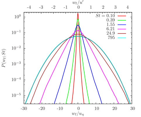
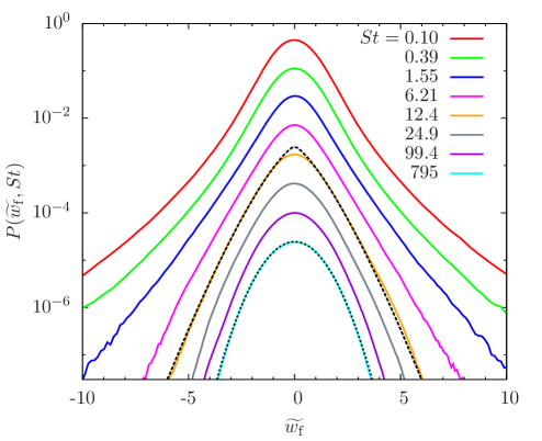
Figure 1.— The PDF of one component, $w_{\rm f}$, of the particle-flow relative velocity as a function of $St$. In the left panel, $w_{\rm f}$ is normalized to $u_{\eta}$ and $u^{\prime}$ on the bottom and top X-axes, respectively. In the right panel, $w_{\rm f}$ is normalized to its rms value (i.e., $\widetilde{w_{\rm f}}\equiv w_{\rm f}/w_{\rm f}^{\prime}$), so that each PDF has a variance of unity. The top curve in this panel plots the actual PDF values for $St=0.1$, and, for clarity, each curve below is shifted downward by a factor of 4. The black dashed line is the stretched exponential fit with $\alpha=4/3$ to the PDF tails of $St=12.4$ particles. In both panels, the black dotted line is the Gaussian fit for the largest particle ($St=795$) in our simulation.

To see the PDF shape more clearly, the right panel of Fig. 1 plots the normalized PDF, $P(\widetilde{w_{\rm f}},\tau_{\rm p})$, with unit variance, where $\widetilde{w_{\rm f}}\equiv w_{\rm f}/w_{\rm f}^{\prime}$, with $w_{\rm f}^{\prime}$ the rms of $w_{\rm f}$. For clarity, we briefly introduce our terminology for the description of the PDF shape. Following Paper I, we use “fat” or “thin” to specifically describe the shape of the PDF, while the extension or width of the PDF, corresponding to the rms, will be described as “broad” or “narrow”. Conventionally, the fatness of a PDF is used as a measure of the departure from a Gaussian distribution, and in particular, it refers to higher probabilities than a Gaussian distribution at the tail part of the PDF. The fatness of a PDF may be quantified, e.g., by its kurtosis, and a fatter PDF has a larger kurtosis. Typically, a larger kurtosis corresponds to a fatter tail part, and at the same time a sharper or thinner shape at the inner part of the PDF. Despite a sharper inner part, the convention is to describe the PDF with a larger kurtosis as fatter based on the tail part. In the right panel of Fig. 1, we see that, for small particles, the PDF is highly non-Gaussian with fat tails. For example, for $St=0.1$, the kurtosis of the PDF is $\simeq 5.6$. As $St$ increases, the PDF shape becomes thinner and thinner. The bottom line in the right panel corresponds to the largest particles ($St=795$) in our simulation, and the PDF for these particles is Gaussian (the black dotted line). In fact, $P(w_{\rm f},\tau_{\rm p})$ becomes close to Gaussian at $St\;\hbox to0.0pt{\lower 2.5pt\hbox{$\sim$}\hss}\raise 1.5pt\hbox{$>$}\;99.4$ (or $\Omega\;\hbox to0.0pt{\lower 2.5pt\hbox{$\sim$}\hss}\raise 1.5pt\hbox{$>$}\;6.9$).

From the PP10 picture, the PDF of ${\boldsymbol{w}}_{\rm f}$ is controlled by the distribution of $\Delta_{\rm T}{\boldsymbol{u}}$, which, however, is unknown. For very small particles with $\tau_{\rm p}\ll\tau_{\eta}$, one may approximate $\Delta_{\rm T}{\boldsymbol{u}}(\Delta\tau)$ by the temporal velocity difference, $\Delta_{\rm L}{\boldsymbol{u}}(\Delta\tau)$, along Lagrangian trajectories of tracers. On the other hand, due to their slow motions, the flow velocity seen by large particles with $\tau_{\rm p}\gg T_{\rm L}$ may be better described as Eulerian, and $\Delta_{\rm T}{\boldsymbol{u}}(\Delta\tau)$ is likely close to the Eulerian temporal flow velocity difference $\Delta_{\rm E}{\boldsymbol{u}}(\Delta\tau)$ at fixed points. In Appendix A, we compute the PDFs of $\Delta_{\rm L}{u}$ and $\Delta_{\rm E}{u}$ in our simulated flow and show that both PDFs are non-Gaussian at small time lags $\Delta\tau$. The PDF tails of both $\Delta_{\rm L}{u}$ and $\Delta_{\rm E}{u}$ have a thinning trend with increasing $\Delta\tau$ and reach Gaussianity at $\Delta\tau\gg T_{\rm L}$ (see, e.g., Mordant et al. 2001, Chevillard et al. 2005). The non-Gaussianity of $\Delta_{\rm L}{u}$ and $\Delta_{\rm E}{u}$ and their trend with $\Delta\tau$ is a well-known phenomenon in turbulent flows, usually referred to as intermittency (e.g., Frisch 1995). The behavior of the PDFs of $\Delta_{\rm L}{u}$ and $\Delta_{\rm E}{u}$ explains the non-Gaussianity of $w_{\rm f}$ and the thinning of $P(w_{\rm f},\tau_{\rm p})$ with increasing $St$. In this sense, the particle-flow relative velocity “inherits” non-Gaussianity from the turbulent flow. From eq. (2), the PDF trend of $w_{\rm f}$ suggests that the distribution of the acceleration contribution ${\boldsymbol{w}}_{\rm a}$ becomes thinner and thinner with increasing $\tau_{\rm p,h}$.

A comparison of the normalized PDF of $w_{\rm f}$ with that of $\Delta_{\rm L}{u}$ (Appendix A) at a time lag $\Delta\tau=\tau_{\rm p}$ shows that, for $St\;\hbox to0.0pt{\lower 2.5pt\hbox{$\sim$}\hss}\raise 1.5pt\hbox{$<$}\;6.21$, the tails of $P(\widetilde{w_{\rm f}},\tau_{\rm p})$ are thinner than $P(\widetilde{\Delta_{\rm L}{u}},\tau_{\rm p})$. The physical reason is that inertial particles do not exactly follow the fluid elements. In particular, inertial particles tend to be pushed out of regions of high vorticity by a centrifugal force arising from the rotation (e.g., Pan et al. 2011). Therefore, they do not experience the flow velocity in strong vortex tubes at small scales, which are intense structures responsible for the high non-Gaussianity (or intermittency) of $\Delta_{\rm L}{u}$ in turbulent flows (Bec et al. 2006). This effect contributes to make the PDF of $w_{\rm f}$ thinner. For particles with $St\;\hbox to0.0pt{\lower 2.5pt\hbox{$\sim$}\hss}\raise 1.5pt\hbox{$>$}\;6.21$, the PDF shape for $w_{\rm f}$ and $\Delta_{\rm L}{u}(\Delta\tau=\tau_{\rm p})$ are close to each other, and this is because both the dynamics of these larger particles and the temporal flow velocity structures at larger timescales are less sensitive to the intense, coherent vortices at small scales.

For all particles, the innermost part of the PDF of $w_{\rm f}$ shows a smooth Gaussian-like shape, suggesting that the PDF of trajectory temporal velocity difference, $\Delta_{\rm T}{\boldsymbol{u}}$, also takes a similar shape in the inner part. This is supported by the observation in Appendix A that the central parts of the PDFs of $\Delta_{\rm L}{u}$ and $\Delta_{\rm E}{u}$ have a more-or-less Gaussian shape. The fat non-Gaussian PDF tails of $w_{\rm f}$ can be fit by stretched exponential functions defined as,

$$P_{\rm se}(x)=\frac{\alpha}{2\beta\Gamma(1/\alpha)}\exp\left[-\left(\frac{|x|}{\beta}\right)^{\alpha}\right],$$ (4)

where $\Gamma$ is the Gamma function (Paper I). The variance of $P_{\rm se}$ is given by $\beta^{2}\Gamma(3/\alpha)/\Gamma(1/\alpha)$. The parameter $\alpha$ controls the fatness of the PDF, and a smaller $\alpha$ corresponds to fatter tails. As expected, the $\alpha$ value for the tails of $P(w_{\rm f},\tau_{\rm p})$ increases with increasing $\tau_{\rm p}$ or $St$. For the eight lines shown in the right panel of Fig. 1, the best-fit $\alpha$ for the PDF tails are 0.7, 0.78, 0.95, 1.23, 1.33, 1.7, 1.95 and 2 for $St=0.10$, 0.39, 1.55, 6.21, 12.4, 24.9, 99.4, and 795, respectively.

The black dashed line in Fig. 1 is the stretched exponential function with $\alpha=\frac{4}{3}$ that best fits the PDF tail of $St=12.4$ particles. The friction time of these particles is close to the Lagrangian correlation time $T_{\rm L}$ of the flow. In Paper I, we found that this stretched exponential can also well fit the relative velocity PDF of equal-size particles with $St=12.4$ and $St=24.7$ (see also §3.2). This similarity in the shape of the PDF tails for ${\boldsymbol{w}}_{\rm f}$ and the monodisperse relative velocity of $\tau_{\rm p}\simeq T_{\rm L}$ particles is of particular interest. Its implication will be discussed in §4.2.1.

Finally, we point our that, if the flow velocity were exactly Gaussian, then the temporal flow velocity difference would be Gaussian, and our model picture indicates that the PDF of the particle-flow relative velocity would be Gaussian for particles of any sizes. In that case, the relative velocity PDF between different particles approaches Gaussian once the generalized acceleration contribution dominates. This suggests that using a Gaussian model flow velocity (see, e.g., Hubbard 2013) to study the particle relative velocity PDF would underestimate the degree of non-Gaussianity.

3.2. Equal-size Particles

The relative velocity PDF of equal-size particles has been discussed in details in Paper I. For convenience, we refer to this monodisperse case with $St_{2}=St_{1}$ as Limit II. In Paper I, we found that the relative velocity PDF of identical particles is extremely non-Gaussian. We identified two sources of non-Gaussianity, i.e., the imprint of the non-Gaussianity (or intermittency) of the turbulent flow and an intrinsic contribution arising from the particle dynamics. Our simulation data showed that the fatness of the monodisperse PDF first increases with $St$, reaches a peak at $St\simeq 1$, and then continuously decreases as $St$ increases above 1. In the following, we briefly review the explanation for this behavior based on the PP10 picture.

For equal-size particles, only the shear term contributes, and the relative velocity, $w$, can be estimated by eq.  (3) for $w_{\rm s}$. For a particle pair with $\tau_{\rm p}\;\hbox to0.0pt{\lower 2.5pt\hbox{$\sim$}\hss}\raise 1.5pt\hbox{$<$}\;T_{\rm L}$, the factor $t_{\rm p}/(t_{\rm p}+\tau_{\rm p})$ in eq. (3) is of oder unity, and, qualitatively, $w$ can be approximated by the spatial flow velocity difference, $\Delta u(r_{\rm p})$, across the primary distance, $r_{\rm p}$ (Paper I). At a given $r$, the primary distance, $r_{\rm p}\simeq(r^{2}+w^{2}\tau_{\rm p}^{2})^{1/2}$, of particle pairs with $|w|\;\hbox to0.0pt{\lower 2.5pt\hbox{$\sim$}\hss}\raise 1.5pt\hbox{$<$}\;r/\tau_{\rm p}$ is close to $r$. Therefore, the inner part of the PDF with $|w|\;\hbox to0.0pt{\lower 2.5pt\hbox{$\sim$}\hss}\raise 1.5pt\hbox{$<$}\;r/\tau_{\rm p}$ follows $\Delta u$ at a distance of $r$. The distribution of $\Delta u$ at small scales is already non-Gaussian (e.g., Frisch 1995), and it leaves a non-Gaussian imprint on the PDF of $w$. Particle pairs lying at higher PDF tails separate faster backward in time and have larger $r_{\rm p}$, so their relative velocity “remembers” $\Delta u(\ell)$ at larger scales $\ell$. Here, $\Delta u(\ell)$ denotes a component of $\Delta{\boldsymbol{u}}({\boldsymbol{\ell}})\equiv{\boldsymbol{u}}({\boldsymbol{x}}+{\boldsymbol{\ell}},t)-{\boldsymbol{u}}({\boldsymbol{x}},t)$ at a separation ${\boldsymbol{\ell}}$. Since the PDF of $\Delta u$ is wider at larger $\ell$, this leads to an enhancement at the tail part of the PDF. The effect, named as a self-amplification in Paper I, corresponds to the sling effect or caustic formation that occurs in flow regions with large velocity gradients, $\partial_{j}u_{i}$ (Falkovich et al. 2002, Wilkinson & Mehlig 2005, Wilkinson et al.  2006, Falkovich & Pumir 2007, Bewley et al. 2013). As $St$ increases, the self-amplification proceeds from the tails toward smaller $|w|$, while the innermost part of the PDF remains unchanged at first. As a result, the overall shape of the PDF becomes fatter.

The fattening trend ends at $St\simeq 1$. As $St$ increases above 1, the amplification moves deeper toward the central part, and the PDF at the same value of $w$ samples $\Delta u$ at larger scales. Since the PDF shape of $\Delta u(\ell)$ is progressively thinner with increasing $\ell$ (see Appendix B of Paper I), this causes the overall fatness of the PDF of $w$ to decrease continuously at $St\;\hbox to0.0pt{\lower 2.5pt\hbox{$\sim$}\hss}\raise 1.5pt\hbox{$>$}\;1$. The PDF shape is thus the fattest at $St\simeq 1$.

For particles with $\tau_{\rm p}$ close to $T_{\rm L}$, the PDF tails of $w$ were found to be well described by a 4/3 stretched exponential distribution (see eq. (4)). Such a distribution were obtained in Paper I from a phenomenological argument based on the PP10 picture. Assuming exactly Gaussian flow velocity and Kolmogorov scaling for $\Delta u(\ell)^{2}\propto C(\bar{\epsilon}\ell)^{2/3}$ with $C$ the Kolmogorov constant, the probability of finding a particle pair with a relative velocity of $w$ is estimated as $\propto\exp[-w^{2}/(2C\bar{\epsilon}^{2/3}(r^{2}+w^{2}\tau_{\rm p}^{2})^{1/3})]$, which is a 4/3 stretched exponential at $w\gg r/\tau_{\rm p}$ (see also Gustavsson et al. 2008). Using the same argument, one can show that non-Gaussianity is an intrinsic feature of the particle dynamics: Even if the flow velocity were exactly Gaussian, the particle relative velocity would be non-Gaussian for any scaling behavior of $\Delta u({\ell})$ with $\ell$ (unless it is constant with $\ell$ as in the case of a white noise).

Finally, for $\tau_{\rm p}\gg T_{\rm L}$, the flow correlation or memory time is typically shorter than the particle memory, and the last factor in eq. (3) reduces the PDF width by a factor of $(T_{\rm L}/\tau_{\rm p})^{1/2}$. In the limit $\tau_{\rm p}\to\infty$, the particle motions are similar to Brownian motion, because even the largest eddies in the flow act as random noise when viewed over the friction time of these large particles. Therefore, the relative velocity PDF is expected to approach Gaussian as $\tau_{\rm p}\to\infty$. A Gaussian shape is almost reached for the largest particles with $\tau_{\rm p}=54T_{\rm L}$ in the simulation of Paper I.

The comparison between Limits I and II at equal $\tau_{\rm p}$ is useful to understand the PDF trend in the general bidisperse case (see §4). For a small particle with $\tau_{\rm p}\to 0$, the PDFs of its relative velocity with respect to the local flow velocity and to a nearby particle of the same size are determined by the distributions of the flow acceleration, ${\boldsymbol{a}}$, and the velocity gradients, $\partial_{j}u_{i}$, respectively (see §2). In Appendix B, we compute the normalized PDFs of ${\boldsymbol{a}}$ and $\partial_{j}u_{i}$ in our simulated flow, and show that the distribution of ${\boldsymbol{a}}$ is generally fatter, consistent with previous studies (e.g., Ishihara et al. 2007). This suggests that, in the $St\to 0$ limit, the PDF of ${\boldsymbol{w}}_{\rm f}$ has a fatter shape than the relative velocity of equal-size particles. As $St$ increases toward $\simeq 1$, the PDF for equal-size particles fattens significantly due to the tail amplification (see discussion above), while the PDF for the particle-flow relative velocity becomes thinner continuously (see Fig. 1). The opposite trends of the two PDFs for $St\;\hbox to0.0pt{\lower 2.5pt\hbox{$\sim$}\hss}\raise 1.5pt\hbox{$<$}\;1$ have an important consequence. The PDF for equal-size particles is found to be already fatter than the distribution of $w_{\rm f}$ at the smallest Stokes number, $St=0.1$, in our simulation, and, at $St\simeq 1$, the former has a much stronger non-Gaussianity than the latter. For $St$ above $1$, the PDF fatness for both cases decreases with increasing $St$, and we will show in §4.1.1 that the relative velocity PDF of equal-size particles remains to be significantly fatter than ${\boldsymbol{w}}_{\rm f}$ at all $St\;\hbox to0.0pt{\lower 2.5pt\hbox{$\sim$}\hss}\raise 1.5pt\hbox{$>$}\;1$. Thus, for all particle species in our simulation, the PDF for Limit II has a higher degree of non-Gaussianity than for Limit I.

3.3. The $\tau_{\rm p2}\to\infty$ Limit and the One-particle Velocity

If one of the two particles, say particle (2), is extremely large with $\tau_{\rm p2}\gg T_{\rm L}$, its velocity is tiny, and the relative velocity with respect to the smaller particle (1) is essentially the one-particle velocity, ${\boldsymbol{v}}^{(1)}$, of particle (1). We refer to this case as Limit III, corresponding to $St_{2}\to\infty$. Paper I found that the PDF of the one-particle velocity, ${\boldsymbol{v}}$, for particles of any size is Gaussian. As discussed in Paper I, this is easy to see in the small and large particle limits. Small particles closely follow the local flow velocity, and the PDF of ${\boldsymbol{v}}$ is approximately given by the 1-point PDF of the flow velocity, ${\boldsymbol{u}}$, which is known to be approximately Gaussian. On the other hand, the motions of large particles with $\tau_{\rm p}\gg T_{\rm L}$ are similar to Brownian motion, because, for these particles, turbulent eddies of all sizes act as random noise when viewed over a timescale of $\simeq\tau_{\rm p}$. Therefore, the one-particle velocity PDF in the large particle limit is also Gaussian. The Gaussianity of the one-particle velocity ${\boldsymbol{v}}$ for particles of any size suggests that, for any given $St_{1}$, the bidisperse relative velocity PDF approaches Gaussian as $St_{2}\to\infty$.

4. The PDF of the Particle Relative Velocity

We analyze the probability distribution function of the particle relative velocity for all Stokes number pairs in our simulation. To compute the relative velocity statistics, we search pairs of particles from all species at given distances, $r$. We will consider $r=1$, $\frac{1}{2}$, and $\frac{1}{4}\eta$. It would be useful to measure the PDF at even smaller $r$ because the size of dust particles in protoplanetary disks is much smaller than the Kolmogorov scale of protoplanetary turbulence. However, the number of particle pairs available in the simulation decreases with decreasing $r$, and, at $r\ll 1\eta$, the number is too limited to provide sufficient statistics. We will thus show simulation results for $\frac{1}{4}\eta\leq r\leq 1\eta$, and discuss the $r-$dependence (or convergence) of the PDF in this range.

For each particle (1), we locate particles (2) in a distance shell $[r-dr/2,r+dr/2]$. The shell thickness, $dr$, is set to $0.08r$, $0.08r$, and $0.16r$ for $r=1$, $\frac{1}{2}$, and $\frac{1}{4}\eta$, respectively. For $r=\frac{1}{4}\eta$ with $dr=0.16r$, the number of particle pairs for any two species is $\;\hbox to0.0pt{\lower 2.5pt\hbox{$\sim$}\hss}\raise 1.5pt\hbox{$>$}\;10^{4}$, about sufficient for the PDF measurement. We examine the PDFs of the radial and tangential components, as well as the 3D amplitude, of the relative velocity. The 3D amplitude is of practical interest as it determines the total collision energy and hence the collision outcome. The PDFs of the radial and tangential components, on the other hand, are helpful for a thorough understanding of the underlying physics. In particular, the features of the radial and tangential PDFs provide very useful tests for the PP10 picture. To obtain the radial and tangential components, we set up a local coordinate system for each selected pair. In terms of the grid base vectors, ${\boldsymbol{e}}_{1}$, ${\boldsymbol{e}}_{2}$, and ${\boldsymbol{e}}_{3}$, the local system is taken to be ${\boldsymbol{e}}^{\prime}_{1}=\cos\theta\cos\phi{\boldsymbol{e}}_{1}+\cos\theta\sin\phi{\boldsymbol{e}}_{2}+\sin\theta{\boldsymbol{e}}_{3}$, ${\boldsymbol{e}}^{\prime}_{2}=-\sin\phi{\boldsymbol{e}}_{1}+\cos\phi{\boldsymbol{e}}_{2}$ and ${\boldsymbol{e}}^{\prime}_{3}=-\sin\theta\cos\phi{\boldsymbol{e}}_{1}-\sin\theta\sin\phi{\boldsymbol{e}}_{2}+\cos\theta{\boldsymbol{e}}_{3}$. The Euler angles are defined as $\sin\theta=r_{3}/r$, $\cos\theta=(r_{1}^{2}+r_{2}^{2})^{1/2}/r$, $\cos\phi=r_{1}/(r_{1}^{2}+r^{2}_{2})^{1/2}$, and $\sin\phi=r_{2}/(r_{1}^{2}+r_{2}^{2})^{1/2}$, with $r_{1}$, $r_{2}$ and $r_{3}$ the components of ${\boldsymbol{r}}$ in the grid coordinate. We decompose ${\boldsymbol{w}}$ as $w_{\rm r}={\boldsymbol{w}}\cdot{\boldsymbol{e}}^{\prime}_{1}$, $w_{\rm t2}={\boldsymbol{w}}\cdot{\boldsymbol{e}}^{\prime}_{2}$, and $w_{\rm t3}={\boldsymbol{w}}\cdot{\boldsymbol{e}}^{\prime}_{3}$. The tangential PDF, $P(w_{\rm t};St_{1},St_{2})$, is set to the average of $P(w_{\rm t2};St_{1},St_{2})$ and of $P(w_{\rm t3};St_{1},St_{2})$. The analysis is the same as in Paper I for equal-size particles. In §4.1, we fix the Stokes number, $St_{1}$, of particles (1), and examine the trend of the relative velocity PDF as a function of $St_{2}$. In §4.2, we will show the PDFs at fixed Stokes number ratios, $f\equiv St_{\ell}/St_{h}$. We will pay particular attention to the non-Gaussianity of the PDF, and discuss how the PDF shape changes with the Stokes numbers. As a reminder, in our terminology, a “fat” (or “thin” ) PDF shape refers to higher (or lower) probabilities specifically at the tail part of the PDF.

4.1. The PDF at Fixed $St_{1}$

If one of the Stokes numbers is fixed at $St_{1}$, the three interesting limits, i.e., $St_{2}\to 0$, $St_{2}=St_{1}$, and $St_{2}\to\infty$, discussed in §3 are useful to confine the trend of the PDF shape as a function of $St_{2}$. These cases were named as limits I, II, and III, respectively. The shape of the PDF for $0\leq St_{2}\leq St_{1}$ is expected to lie in between Limit I and Limit II, while $St_{1}\leq St_{2}<\infty$ corresponds to a range between Limits II and III.

4.1.1 The PDFs of the radial and tangential relative speeds

In Fig. 2, we plot the PDFs, $P(w_{\rm r};St_{1},St_{2})$, of the radial relative velocity for $St_{1}$ fixed at $1.55$. The relative velocity is measured at $r=1\eta$. The left and right panels show results for $St_{2}\leq St_{1}$ and $St_{2}\geq St_{1}$, respectively. In both panels, the solid black line is the PDF for identical particles with $St=1.55$, corresponding to Limit II. The monodisperse PDF at $St=1.55$ is highly non-Gaussian, and the physical origin of the non-Gaussianity has been explained in §3.2 using the PP10 picture. This PDF is also negatively skewed. The left and right wings of the PDF correspond to approaching and separating particle pairs. The asymmetry of the two wings indicates faster relative velocity for approaching pairs. As discussed in Paper I, there are two reasons for this asymmetry. First, the radial relative speed PDF for small equal-size particles inherits a negative skewness from the PDF of the longitudinal flow velocity difference or gradients of the flow (see Appendix B and Paper I). Second, approaching particle pairs have a larger separation in the near past than separating pairs. This suggests that, for small particles, the primary distance, $r_{\rm p}$, of approaching pairs is larger than separating ones, which enhances the asymmetry as $St$ increases at small $St\;\hbox to0.0pt{\lower 2.5pt\hbox{$\sim$}\hss}\raise 1.5pt\hbox{$<$}\;1$. As $St$ keeps increasing, the particle distance ($r_{\rm p}$) at a friction time ago is less dependent of the particle separation in the near past, and the asymmetry decreases (see Figs. 4 and 5).

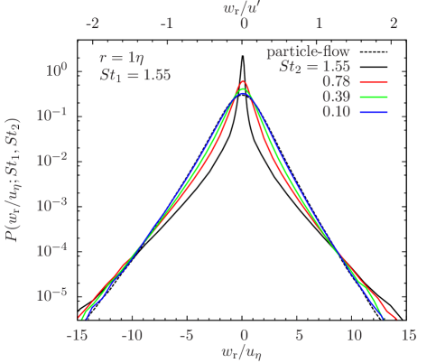
Figure 2.— PDF of the radial relative speed at $r=1\eta$ as a function of $St_{2}$ for $St_{1}=1.55$. The left and right panels show results for $St_{2}\leq St_{1}$ and $St_{2}\geq St_{1}$, respectively. The solid black curves in both panels correspond to the same monodisperse PDF at $St=1.55$. Note that, for clarity of the PDF shapes for $St_{2}\leq St_{1}$, the left panel shows a narrower range of $w_{\rm r}$ than in the right panel. The dashed black line in the left panel is the PDF of the particle-flow relative velocity of $St=1.55$ particles, while the dashed line in the right panel shows the best-fit Gaussian PDF for $St_{1}=1.55$ and $St_{2}=795$.

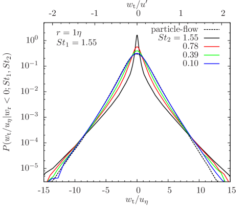
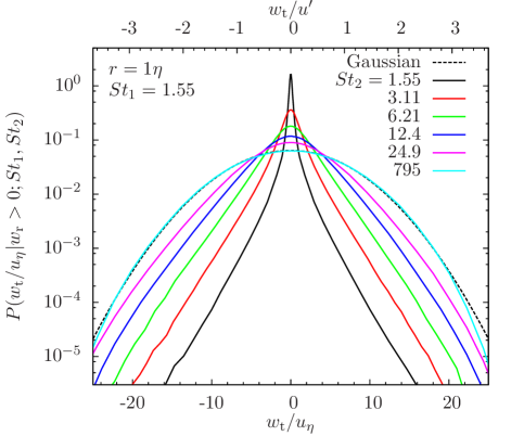
Figure 3.— PDF of the tangential relative velocity for approaching particle pairs ($w_{\rm r}<0$) with one of the Stokes number $St_{1}$ fixed at $1.55$. The figure is plot in the same way as Figure 2.

The black dashed line in the left panel plots the PDF of the radial component, $w_{\rm f,r}$, of the relative velocity between $St=1.55$ particles and the flow element, corresponding to Limit I with $St_{1}=1.55$ and $St_{2}\to 0$. For a consistent comparison with the particle-particle case, here the PDF of $w_{\rm f,r}$ is measured at the same distance, $r=1\eta$. It is thus not the same as the particle-flow relative velocity PDFs shown in Fig. 1 at zero distance. To compute $w_{\rm f,r}$ at a finite distance, we used the TSC interpolation to obtain the flow velocities at a separation of $r$ from the position of each particle in the three base directions of the simulation grid. We then averaged the PDFs of $w_{\rm f,r}$ measured from the three directions. Unlike the particle-flow relative velocity at zero distance, here the PDF of $w_{\rm f,r}$ at $r=1\eta$ for $St=1.55$ is asymmetric. This is because, at a finite distance, the generalized shear term has a nonzero contribution (see eq. 3) to the relative velocity, which gives rise to a noticeable negative skewness in the PDF of $w_{\rm f,r}$ for small particles with $St\;\hbox to0.0pt{\lower 2.5pt\hbox{$\sim$}\hss}\raise 1.5pt\hbox{$<$}\;3.11$.

As expected, the bidisperse PDFs in the left panel of Fig. 2 lie in between Limit II (black solid line) and Limit I (dashed solid line). Since a negative skewness exists in both limits, the PDF is asymmetric for all $St_{2}\leq St_{1}$. At the smallest $St_{2}$ ($=0.1$; the blue line) shown in the figure, the radial PDF, $P(w_{\rm r};St_{1},St_{2})$, approaches Limit I. As $St_{2}$ decreases below $St_{1}$, the central part of the PDF widens, and the rms of the PDF increases (Paper II). This corresponds to the increase in the contribution of the generalized acceleration term, ${\boldsymbol{w}}_{\rm a}$. As discussed in §2, ${\boldsymbol{w}}_{\rm a}$ is related to the temporal flow velocity difference, $\Delta_{\rm T}{\boldsymbol{u}}$, on the particle trajectory. Applying eq. (2) to the Stokes number pairs in the left panel of Fig. 2, we have ${\boldsymbol{w}}_{\rm a}\simeq(1-f)\Delta_{\rm T}{\boldsymbol{u}}(\tau_{\rm p1})$, where $f=St_{2}/St_{1}$ for $St_{2}\leq St_{1}$. Clearly, as $St_{2}$ decreases, $f$ decreases and the contribution of ${\boldsymbol{w}}_{\rm a}$ increases. On the other hand, it can be seen from eq. (3) that the shear contribution decreases with decreasing $St_{2}$ (see Paper II).

The black solid line for Limit II has a fatter overall shape than the black dashed line for Limit II (see the discussion at the end of §3.2), suggesting that the distribution of the generalized acceleration contribution is thinner than the shear contribution. As ${\boldsymbol{w}}_{\rm a}$ increases with decreasing $St_{2}$, the overall fatness of the relative velocity PDF decreases. Interestingly, despite the increase in the rms width, the probability at the far tails of the relative velocity PDF becomes smaller at smaller $St_{2}$, indicating a lower probability of finding particle pairs that collide with extremely high velocity. In general, whether the probability at the far tails increases or decreases with decreasing $St_{2}$ is determined by the competition of two effects. First, if the PDF shape is given, an increase in the rms tends to give a larger probability at the far tails. On the other hand, if the rms is fixed, the thinning of the PDF shape would lead to a lower probability at high tails. It appears that the effect of thinning PDF shape wins in the case of $St_{1}=1.55$ and $St_{2}\leq St_{1}$.

The right panel of Fig. 2 shows the radial relative speed PDF for $St_{2}\geq St_{1}=1.55$. As $St_{2}$ increases, the PDF becomes wider, and its shape becomes thinner. This is again due to the increase in the contribution from the acceleration term. Using eq. (2) here, we have ${\boldsymbol{w}}_{\rm a}\simeq(1-f)\Delta_{\rm T}{\boldsymbol{u}}(\tau_{\rm p2})$, where $f=St_{1}/St_{2}$. As $St_{2}$ increases, both the time lag in $\Delta_{\rm T}{\boldsymbol{u}}$ and the factor $1-f$ increase, leading to the increase of the rms width of the PDF. The PDF shape of $\Delta_{\rm T}{\boldsymbol{u}}(\tau_{\rm p2})$ is expected to become thinner with increasing $\tau_{\rm p2}$. This is based on the observation of the thinning trend of the Eulerian and Lagrangian temporal velocity differences with increasing time lag $\Delta\tau$ (see Appendix A). The argument was used earlier to explain the thinning trend of the particle-flow relative velocity with particle inertia (see §3.1). The thinning of the distribution of $\Delta_{\rm T}{\boldsymbol{u}}(\tau_{\rm p2})$ with increasing $St_{2}$ makes the PDF of the relative velocity thinner. At $St_{2}\geq 49.7$, the PDF is close to Gaussian, consistent with the expectation for Limit III (§2.3). The black dashed line in the figure is the Gaussian fit to the $St_{2}=795$ case. We note that the PDF becomes symmetric for $St_{2}\;\hbox to0.0pt{\lower 2.5pt\hbox{$\sim$}\hss}\raise 1.5pt\hbox{$>$}\;6.21$.

Since the PDF shape becomes thinner for $St_{2}$ both above or below $St_{1}$, the fatness of the PDF peaks at equal-size particles. The PDF shapes in both limits I and III are thinner than Limit II. A computation of the skewness of the radial PDFs shows that it decreases as the Stokes number difference increases. This is because the generalized acceleration is independent of the relative motions of the two particles and thus provides a symmetric contribution to the two wings of the radial relative velocity PDF (see discussion in §2).

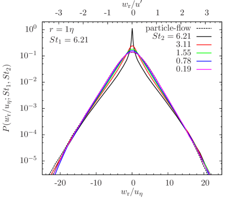
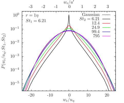
Figure 4.— PDF of the radial relative speed as a function of $St_{2}$ for $St_{1}=6.21$. The figure is plot in the same way as Fig. 2. The dashed black line in the right panel shows the best Gaussian fit to the bidisperse PDF for $St_{2}=795$.

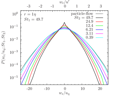
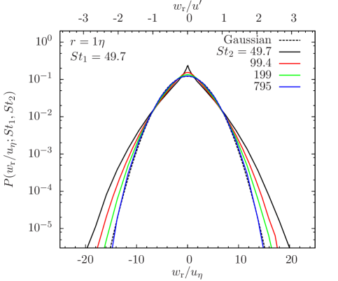
Figure 5.— Same as Figure 4, but for $St_{1}=49.7$.

In Fig. 3, we show the PDF of the tangential relative speed, $P(w_{\rm t}|w_{\rm r}\leq 0;St_{1},St_{2})$ at a distance of $r=1\eta$ for $St_{1}=1.55$. The conditioning on a negative radial relative speed ($w_{\rm r}\leq 0$) indicates that only particle pairs approaching each other are counted. Since only approaching particles may lead to collisions, it is of practical interest to separate them out from the pairs moving away from each other. Fig. 3 is plot in the same way as Fig. 2. The trend of $P(w_{\rm t}|w_{\rm r}\leq 0;St_{1},St_{2})$ as a function of $St_{2}$ is similar to that of $P(w_{\rm r};St_{1},St_{2})$. Unlike the radial component, the two wings of the tangential PDF are symmetric, as expected from statistical isotropy. We find that, for any $St_{2}$, the left wing of $P(w_{\rm r};St_{1},St_{2})$ coincides with that of $P(w_{\rm t}|w_{\rm r}\leq 0;St_{1},St_{2})$. The coincidence in the monodisperse case was found in Paper I for all particles with $St\;\hbox to0.0pt{\lower 2.5pt\hbox{$\sim$}\hss}\raise 1.5pt\hbox{$>$}\;0.1$ in our simulation. For the bidisperse case, the generalized acceleration term gives equal contributions to $w_{\rm r}$ and $w_{\rm t}$ (§2), and it thus enhances the equalization of the radial and tangential PDF.

The central part of the monodipserse PDF is very sharp with a cusp-like shape (see also Fig. 4 for the $St_{1}=6.21$ case, where the cusp in the monodisperse PDF is even sharper). In the bidisperse case, the central cusp smoothes rapidly as the Stokes number difference increases. This is caused by the contribution of the acceleration term. As argued in §3.1, the PDF of the temporal trajectory velocity difference, $\Delta_{\rm T}{\boldsymbol{u}}$, is expected to take a smooth, Gaussian-like shape in the innermost part. Then, since ${\boldsymbol{w}}_{\rm a}\propto\Delta_{\rm T}{\boldsymbol{u}}$ (eq. (2)), the bidisperse PDF would have a smoother central part, when the acceleration contribution increases.

Fig. 4 plots the PDF of the radial relative velocity for $St_{1}=6.21$. The figure is plot in the same way as Fig. 2 for the radial PDF for $St_{1}=1.55$. As found in Paper I, the fatness of the PDF shape for identical particles decreases with $St$ for $St\;\hbox to0.0pt{\lower 2.5pt\hbox{$\sim$}\hss}\raise 1.5pt\hbox{$>$}\;1$, and the tails of the monodisperse PDF (the black solid lines) for $St\geq 6.21$ are thinner than the $St_{1}=1.55$ case shown in Fig. 2 (see explanation in §3.2). At $St\geq 6.21$, the skewness for the monodisperse radial PDF disappears. An explanation for the recovery of the symmetry at large $St$ was discussed earlier in this section.

Similar to the $St_{1}=1.55$ case, the rms width of the PDF increases as $St_{2}$ decreases below or increases above $St_{1}$, while the overall shape of the PDF becomes thinner. Interestingly, in the left panel, the high PDF tails almost coincide for all $St_{2}$ below $St_{1}$. In particular, the far tails in the dashed black line for Limit I (i.e., the particle-flow relative velocity) happen to be close to those in the black solid line for equal-size particles. As mentioned earlier, two effects, i.e., the increase of the rms and the thinning of the overall PDF shape with decreasing $St_{2}$, determine the trend of the probability at the far tails. The coincidence of the far tails suggests that, at $St_{1}=6.21$, these two effects roughly cancel out. In the right panel, as $St_{2}$ increases above $St_{1}=6.21$, the PDF keeps widening, and the PDF shape approaches Gaussian (the black dashed line) at $St_{2}\;\hbox to0.0pt{\lower 2.5pt\hbox{$\sim$}\hss}\raise 1.5pt\hbox{$>$}\;99.4$.

Fig. 5 plots the PDF of the radial relative velocity for $St_{1}=49.7$. In the left panel, we see that the PDF width increases with decreasing $St_{2}$. The widening of the PDF width wins over the thinning trends of the overall PDF shape with decreasing $St_{2}$, and thus the probability at the far tails keeps increasing with decreasing $St_{2}$. In the right panel, the PDF becomes thinner as $St_{2}$ increases above $St_{1}$, and finally approaches Gaussian, as expected for Limit III. The rms width of all PDFs shown in this panel is almost the same.

To summarize, for a given $St_{1}$, the tail shape of the relative velocity PDF is the fattest for the monodisperse case with $St_{2}=St_{1}$. As $St_{2}$ increase above or decreases below $St_{1}$, the generalized acceleration contribution increases, and the overall PDF shape becomes thinner.

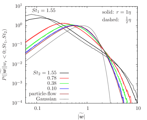
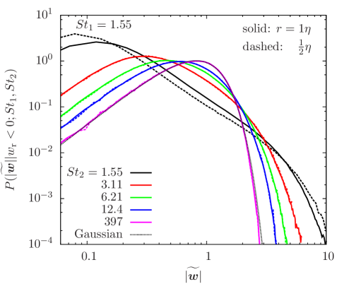
Figure 6.— Normalized PDF of the 3D amplitude, $|{\boldsymbol{w}}|$, of the relative velocity of approaching particle pairs ($w_{\rm r}<0$) at $r=1\eta$ (solid lines) and $\frac{1}{2}\eta$ (dashed lines). In both panels, black lines correspond to identical particles with $St_{2}=St_{1}=1.55$. For each $St_{2}$, the amplitude, $|{\boldsymbol{w}}|$, is normalized to its rms value. Left and right panels show results for $St_{2}\leq St_{1}$ and $St_{2}\geq St_{1}$, respectively. In the left panel, the brown lines are the normalized PDFs of the particle-flow relative velocity at $r=1\eta$ and $\frac{1}{2}\eta$. Black dotted lines in both panels are the normalized PDF, $\sqrt{\frac{54}{\pi}}\widetilde{|{\boldsymbol{w}}|}^{2}\exp(-3\widetilde{|{\boldsymbol{w}}|}^{2}/2)$, for the amplitude of a 3D Gaussian vector.

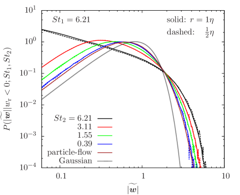
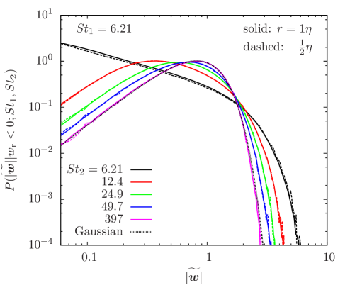
Figure 7.— Similar to Fig. 6, but for $St_{1}=6.21$.

An important conclusion of theoretical interest is that the distribution of the generalized shear contribution, ${\boldsymbol{w}}_{\rm s}$, is fatter than the acceleration term, ${\boldsymbol{w}}_{\rm a}$. This is seen from a comparison of Limits I (black dashed lines) and II (black solid lines) in Figs.  2, 4 and 5, which are dominated by the generalized acceleration and shear terms, respectively. Since ${\boldsymbol{w}}_{\rm a}$ and ${\boldsymbol{w}}_{\rm s}$ are related to the temporal ($\Delta_{\rm T}{\boldsymbol{u}}$) and spatial ($\Delta{\boldsymbol{u}}$) flow velocity differences, respectively, one may understand their distributions by considering the statistics of spatial and temporal velocity structures in turbulence. We first note that the spatial velocity structures in turbulent flows do not have a higher degree of non-Gaussianity than the temporal structures. In fact, the Lagrangian temporal structures are known to be more intermittent than the Eulerian spatial structures (see Appendix A). Therefore, the finding that the distribution of ${\boldsymbol{w}}_{\rm s}$ is fatter than ${\boldsymbol{w}}_{\rm a}$ cannot be interpreted by a simple comparison of the temporal and spatial intermittency. A key to understand the fatter distribution of ${\boldsymbol{w}}_{\rm s}$ is that ${\boldsymbol{w}}_{\rm s}$ and ${\boldsymbol{w}}_{\rm a}$ sample the temporal and spatial flow velocity differences in different ways. Unlike the PDF of ${\boldsymbol{w}}_{\rm a}$, which roughly samples $\Delta_{\rm T}{\boldsymbol{u}}(\Delta\tau)$ at a single time lag $\Delta\tau\simeq\tau_{\rm p,h}$, ${\boldsymbol{w}}_{\rm s}$ is not controlled by the spatial flow velocity difference, $\Delta{\boldsymbol{u}}$, at a single length scale. In fact, different parts of the distribution of ${\boldsymbol{w}}_{\rm s}$ sample the flow velocity at different scales. For example, in the case of equal-size particles with a friction time of $\tau_{\rm p}$, the PDF at relative velocities below/above the rms value, i.e., at $|w|\lessgtr\langle w^{2}\rangle^{1/2}$, depends on the flow velocity at scales $\ell\lessgtr(r^{2}+\langle w^{2}\rangle\tau_{\rm p}^{2})^{1/2}$, respectively. Considering that the PDF width of $\Delta{\boldsymbol{u}}$ increases with increasing $\ell$, this implies that the PDF shape of ${\boldsymbol{w}}_{\rm s}$ is significantly fatter than the PDF of $\Delta{\boldsymbol{u}}$ at a single scale $\ell\simeq(r^{2}+\langle w^{2}\rangle\tau_{\rm p}^{2})^{1/2}$. This fattening effect is responsible for why the distribution of ${\boldsymbol{w}}_{\rm s}$ has a higher degree of non-Gaussianity than ${\boldsymbol{w}}_{\rm a}$, even though the spatial flow velocity structures are not more intermittent than the temporal ones.

4.1.2 The PDF of the 3D amplitude

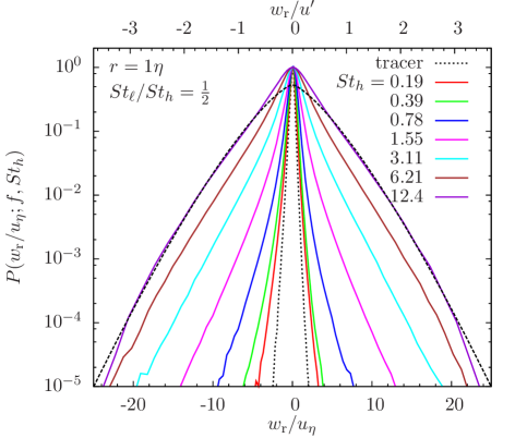
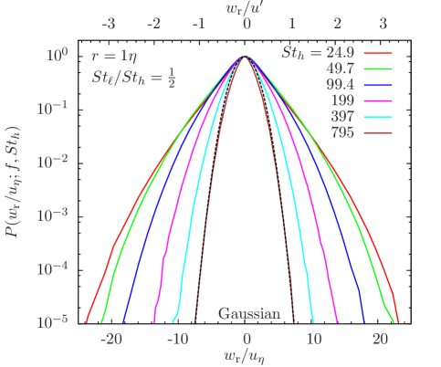
Figure 8.— PDF of the radial relative velocity at $r=1\eta$ for a Stokes ratio $f=\frac{1}{2}$. Left and right panels show $St_{h}\leq 12.4$ and $St_{h}>12.4$, respectively. All PDFs are normalized to the central peak values. The black dashed line in the left panel corresponds to the PDF of tracer particles, while the long dashed line is the stretched exponential fit with $\alpha=4/3$ to the PDF tails for $St_{h}=12.4$. The black dashed line in the right panel is the Gaussian fit to the PDF of the two largest particles in our simulation.

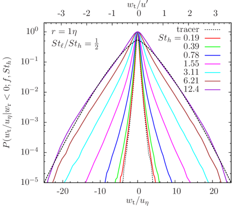
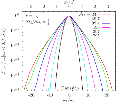
Figure 9.— The PDF of the tangential relative velocity at $r=1\eta$ for a Stokes ratio of $f=\frac{1}{2}$. The figure is plot in the same way as Fig. 8 for the radial PDF.

In Fig. 6, we show the PDF of the 3D amplitude, $|{\boldsymbol{w}}|$, of the relative velocity of approaching particles with $w_{\rm r}<0$. In both panels, $St_{1}$ is fixed at $1.55$, and the left and right panels plot the PDFs for $St_{2}\leq St_{1}$ and $St_{2}\geq St_{1}$, respectively. We normalized $|{\boldsymbol{w}}|$ to its rms value, i.e., $\widetilde{|{\boldsymbol{w}}|}\equiv|{\boldsymbol{w}}|/\langle w^{2}\rangle_{-}^{1/2}$, where $\langle w^{2}\rangle_{-}^{1/2}$ is the 3D rms relative velocity of approaching particle pairs with negative $w_{\rm r}$. As discussed in Paper I, $|{\boldsymbol{w}}|$ is related to the particle collisional energy and its PDF plays an important role in determining the collision outcome.

In both panels of Fig. 6, the solid and dashed black curves show the PDFs of equal-size particles with $St=1.55$ at $r=1$ and $\frac{1}{2}\eta$, respectively. The black dotted lines correspond to the normalized PDF for the amplitude of a 3D Gaussian vector. As shown in Paper I, the monodipserse PDF is extremely non-Gaussian, with large probabilities distributed at both very small and large relative speeds. The large probabilities at small $\widetilde{|{\boldsymbol{w}}|}$($\ll 1$) correspond to the sharp cusps at the central parts of the radial and tangential PDFs (see Figs. 2 and 3). The solid and dashed color curves are bidisperse PDFs at $r=1$ and $\frac{1}{2}\eta$, respectively. As $St_{2}$ moves away from $St_{1}$, the degree of non-Gaussianity in the PDF decreases, consistent with the results in §4.1.1. When the Stokes numbers differ by a factor of 2, there is a rapid decrease in the probability at the left tail. This is because, due to the acceleration contribution, the central parts of the radial and tangential PDFs become smooth and the sharp central cusps disappear (see §4.1.1). As the Stokes number difference increases, the right PDF tail of $\widetilde{|{\boldsymbol{w}}|}$ become thinner, and we also see that the peak of the PDF moves to the right toward $\widetilde{|\boldsymbol{w}|}\simeq 1$, meaning that more probabilities are distributed around the rms relative velocity. In the left panel, as $St_{2}$ decreases to $0.1$, the PDF shape approaches that of the particle-flow relative velocity (brown lines), which is still fatter than Gaussian (the black dotted line). In the right panel, the PDF of $|{\boldsymbol{w}}|$ approaches Gaussian in the limit of large $St_{2}$. At $St_{2}\;\hbox to0.0pt{\lower 2.5pt\hbox{$\sim$}\hss}\raise 1.5pt\hbox{$>$}\;398$, the PDF coincides with the Gaussian distribution. The trend of the PDF shape as a function of $St_{2}$ is again consistent with the expectation that it lies in between the three limits, $St_{2}\to 0$, $St_{2}=St_{1}$ and $St_{2}\to\infty$. Fig. 7 shows the simulation result for $St_{1}=6.21$, which is similar to Fig. 6 for the $St_{1}=1.55$ case.

In the monodisperse case, the PDF converges with decreasing $r$ already at $r\simeq 1\eta$, for particles with $St\;\hbox to0.0pt{\lower 2.5pt\hbox{$\sim$}\hss}\raise 1.5pt\hbox{$>$}\;6.21$ (see black solid and dashed lines in Fig. 7). However, for smaller particles of equal-size with $St\;\hbox to0.0pt{\lower 2.5pt\hbox{$\sim$}\hss}\raise 1.5pt\hbox{$<$}\;3.11$, the PDF shape has an $r-$dependence at $r\simeq\frac{1}{2}\eta$ (see Fig. 6). The convergence for the PDF of identical particles of small size is very challenging to reach, e.g., in the study of Lanotte et al. (2011), the convergence is barely reached at $r\simeq 0.086\eta$ for particles with $St=3.3$. In the bidisperse case, the convergence is easier to achieve because the contribution from the generalized acceleration term is $r-$independent (see §2 and Paper II). All the bidisperse PDFs for different particles shown in Figs. 6 and Fig. 7 already converge at $\frac{1}{2}\eta$. In fact, we find that, except for the two smallest particles with $St_{1}=0.1$ and $St_{2}=0.19$ in our simulation (see Fig. 14 in §4.2.4), the convergence of the PDF shape is reached at $r\simeq\frac{1}{2}\eta$ for all non-equal Stokes pairs.

4.2. The Relative Velocity PDF at Fixed Stokes Ratios

In this subsection, we examine the relative velocity PDF for particle pairs with fixed Stokes number ratios, $f\equiv St_{\ell}/St_{h}$, and show how the PDF changes with $St_{h}$. As a reminder, $St_{\ell}$ and $St_{h}$ are the Stokes numbers of the smaller and larger particles, respectively. With a fixed $f$, it is easier to compare the bidisperse PDF with that of equal-size particles ($f=1$) discussed in Paper I. At a given $f$, there are two interesting limits, $St_{h}\to 0$ and $St_{h}\to\infty$. For $St_{h}\to 0$, both particles become tracers, and the particle relative velocity PDF approaches the PDF, $P_{\rm u}(r)$, of the flow velocity difference, $\Delta u$, across the particle distance, $r$. In the opposite limit $St_{h}\to\infty$, the relative velocity is essentially the 1-particle velocity of the smaller particle, and its PDF approaches Gaussian (§3.3). A particularly interesting result we find is that, if the friction time $\tau_{\rm ph}$ of the larger particle is close to the Lagrangian correlation time $T_{\rm L}$ of the flow, the PDF tails can be approximately described by a 4/3 stretched exponential for any value of $f$.

4.2.1 The PDFs of the radial and tangential relative speeds

In Fig. 8, we show the PDF, $P(w_{\rm r};f,St_{h})$, of the radial relative velocity at $r=1\eta$ for a Stokes ratio of $f=\frac{1}{2}$. The left and right panels plot results for $St_{h}\leq 12.4$ and $St_{h}\geq 24.9$, respectively. Each PDF is normalized to its value at the central peak (i.e., at $w=0$). In the left panel, the black short-dashed line is the PDF of the radial relative velocity between tracer particles (i.e., $St_{h}=0$) at $r=1\eta$, and the long-dashed line is the stretched exponential function with $\alpha=4/3$ (see eq. (4)) that best fits the PDF tails for $St_{h}=12.4$. The dashed line in the right panel is the Gaussian fit for $St_{\ell}=397$ and $St_{h}=795$. The figure is plot in the same way as Fig. 10 of Paper I for the monodisperse case (i.e., $f=1$). The PDF width first increases with $St_{h}$, corresponding to the increase of $\Delta_{\rm T}{\boldsymbol{u}}(\tau_{\rm p,h})$ with $\tau_{\rm p,h}$ in the generalized acceleration term (eq. (2)) and the increase of $r_{\rm p}$ with $\tau_{\rm p,l}$ in the shear term (eq. (3)). But for large $\tau_{\rm p,l}$ and $\tau_{\rm p,h}$, the $(1+\Omega_{\rm l})^{-1/2}$ and $[t_{\rm p}/(t_{\rm p}+\tau_{\rm p,h})]^{1/2}$ factors in eqs. (2) and (3) take effect, leading to the decrease of the PDF width at $\tau_{\rm p,h}\gg T_{\rm L}\simeq 14.4\tau_{\eta}$ (the right panel). The behavior of the width or rms of the PDF at fixed $f$ as a function of $St_{h}$ has been studied and explained in Paper II in the context of the PP10 picture. The left and right wings are asymmetric due to the shear contribution. The asymmetry first increases with $St_{h}$ as $St_{h}$ increases to 0.39, then decreases at larger $St_{h}$. This is similar to the case of equal-size particles ($f=1$; see Paper I) and consistent with the expected behavior of the shear contribution (see a physical discussion in §4.1.1). The PDF reaches symmetry at $St_{h}\;\hbox to0.0pt{\lower 2.5pt\hbox{$\sim$}\hss}\raise 1.5pt\hbox{$>$}\;3.11$.

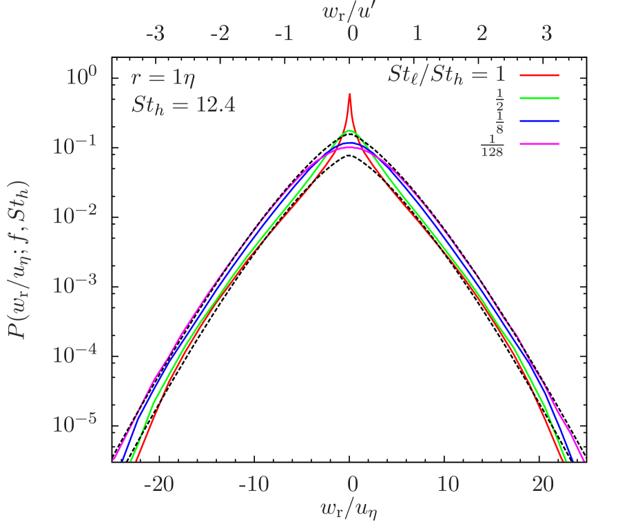
Figure 10.— Radial relative velocity PDF for $St_{h}=12.4$ and $f=1$, $\frac{1}{2}$, $\frac{1}{8}$, and $f\frac{1}{128}$. The friction time of $St_{h}=12.4$ particles is close to the Lagrangian correlation time, $T_{\rm L}$, of the flow. Black dashed lines are stretched exponential fits with $\alpha=4/3$ to the PDF tails for $f=1$ and $\frac{1}{128}$, respectively.

A comparison of the left panel of Fig. 8 with that of Fig. 10 in Paper I for identical particles reveals an interesting difference. As explained in §3.2 (see Paper I for details), in the monodisperse case, the innermost part of the PDF closely follows the flow velocity difference PDF (the short-dashed line for tracers in Fig. 10 of Paper I). On the other hand, the central part of the bidisperse PDF at any $St_{h}$ in the left panel of Fig. 8 is wider than the short-dashed line for tracers. This is because the generalized acceleration term, which is absent for equal-size particles, contributes to the central part of the bidisperse PDF. Also, at the same $St_{h}$, the PDF shape for $f=\frac{1}{2}$ is thinner than for the case of equal-size particles with $f=1$ (see §4.1.1 and also §4.2.3 below).

In Fig. 9, we show the PDF of the tangential relative velocity, $P(w_{\rm t}|w_{\rm r}\leq 0;f,St_{h})$, for approaching particle pairs with $f=\frac{1}{2}$. The figure is plot in the same way as Fig. 8 for the radial case. The two wings of the tangential PDF are symmetric for any $St_{h}$. The tangential PDF as a function of $St_{h}$ shows a similar trend as the case of the radial relative speed (Fig. 8). We find again that the left wings of the radial PDF and the tangential PDF, $P(w_{\rm t}|w_{\rm r}\leq 0;f,St_{h})$, of approaching pairs coincide (see §4.1.1). In Appendix C, we consider the tangential PDF, $P(w_{\rm t}|w_{\rm r}>0;f,St_{h})$, of separating particle pairs (with $w_{\rm r}>0$), and compare it with $P(w_{\rm t}|w_{\rm r}\leq 0;f,St_{h})$. Similar to the asymmetric wings of the radial PDF, for small particles of similar sizes there is a difference between $P(w_{\rm t}|w_{\rm r}\leq 0;f,St_{h})$ and $P(w_{\rm t}|w_{\rm r}>0;f,St_{h})$ for approaching and separating pairs.

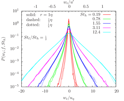
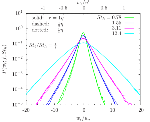
Figure 11.— The radial relative velocity PDF for particle pairs with $f=\frac{1}{2}$ (left panel) and $\frac{1}{8}$ (right panel) at $r=1\eta$ (solid), $\frac{1}{2}\eta$ (dashed), and $\frac{1}{4}\eta$ (dotted).

We also examined the PDFs for other values of $f$. The qualitative behavior of the PDF for different $f$ with increasing $St_{h}$ is similar to the case of $f=\frac{1}{2}$. In §4.2.3, we will carry out a detailed quantitative analysis of the fatness of the PDF shape as a function of $St_{h}$ at a few values of $f$.

In Paper I, we showed that the PDF tails for identical particles with $St=12.4$ and $24.9$ ($\tau_{\rm p}\sim T_{\rm L}$) can be well described by a stretched exponential function with $\alpha=4/3$. A phenomenological argument for this stretched exponential based on the PP10 model was given in §3.2 (see also Paper I). From Figs. 8 and 9, we see that such a stretched exponential fits well the PDF tails also in the bidisperse case with $f=\frac{1}{2}$ and $St_{h}=12.4$. The applicability of the $4/3$ stretched exponential is actually even more general. In Fig.  10, we show the radial PDFs for $St_{h}=12.4$ at 4 values of $f$ in the range $\frac{1}{128}\leq f\leq 1$. The shape of the PDF tails is more or less invariant with $f$, and can be generally approximated by the 4/3 stretched exponential. In other words, a 4/3 stretched exponential applies as long as the friction time of the larger particle is close to $T_{\rm L}$. However, note that, despite the invariance of the tail shape, the central part and hence the overall shape do vary with $f$.

In §3.1, we observed that the particle-flow relative velocity, ${\boldsymbol{w}}_{\rm f}$, (corresponding to $f=0$) for $St=12.4$ particles (see Fig. 1) shows 4/3 stretched exponential tails. Since ${\boldsymbol{w}}_{\rm f}$ is largely controlled by the temporal flow velocity difference, $\Delta{\boldsymbol{u}}_{\rm T}$, along the particle trajectory, this suggests that, for particles with $\tau_{\rm p}\simeq T_{\rm L}$, the PDF tails of $\Delta{\boldsymbol{u}}_{\rm T}(\Delta\tau)$ at $\Delta\tau\simeq T_{\rm L}$ are close to a 4/3 stretched exponential. Then, one may infer from eq. (2) that the acceleration term ${\boldsymbol{w}}_{\rm a}$ ($\propto\Delta{\boldsymbol{u}}_{\rm T}$) would have 4/3 stretched exponential tails if the friction time of the larger particle, $\tau_{\rm p,h}$, is close to $T_{\rm L}$. Considering that it fits well also the PDF tails of the generalized shear term, ${\boldsymbol{w}}_{\rm s}$, in the monodisperse case ($f=1$) with $\tau_{\rm p}\simeq T_{\rm L}$, we would expect that the 4/3 stretched exponential applies to any $f$ as long as $\tau_{\rm p,h}\simeq T_{\rm L}$. The general validity of the 4/3 stretched exponential for $\tau_{\rm p,h}\simeq T_{\rm L}$ may have a profound physical origin, which, however, is currently not clear to us.

4.2.2 The $r-$dependence of the radial relative velocity PDF

Fig. 11 shows the $r-$dependence of the radial PDF for $f=\frac{1}{2}$ (left panel) and $f=\frac{1}{8}$ (right panel). As discussed in §2, the generalized acceleration contribution only depends on individual trajectories of the two particles and is thus $r-$independent. The $r-$dependence of the relative velocity PDF comes only from the shear contribution. In the left panel for $f=\frac{1}{2}$, the PDF width decreases with decreasing $r$ for the smallest $St_{h}$ ($=0.19$). For small particles, the shear term depends on the local flow velocity difference, and thus decreases with decreasing $r$. As $St_{h}$ increases, the $r-$dependence of the PDF width becomes weaker, and in both panels the PDF is almost $r-$independent for $St_{h}\;\hbox to0.0pt{\lower 2.5pt\hbox{$\sim$}\hss}\raise 1.5pt\hbox{$>$}\;3.11$. For larger $St_{\ell}$ and $St_{h}$, the particle memory time is longer, and the particle distance at a friction/memory time ago is less sensitive to $r$. Therefore, the shear contribution becomes less dependent on $r$. At the same time, the increase of the acceleration contribution with $St_{h}$ also tends to reduce the $r-$dependence. A comparison of the left and right panels shows that, at the same $St_{h}$, the $r-$dependence of the PDF is weaker for smaller $f$, again due to the relatively larger acceleration contribution. The $r-$dependence for $f=\frac{1}{2}$ and $\frac{1}{8}$ shown here is much weaker than the equal-size case ($f=1$). It appears that, for $f=\frac{1}{8}$, the PDF already converges at $r=\frac{1}{4}\eta$ for all $St_{h}\;\hbox to0.0pt{\lower 2.5pt\hbox{$\sim$}\hss}\raise 1.5pt\hbox{$>$}\;0.78$.

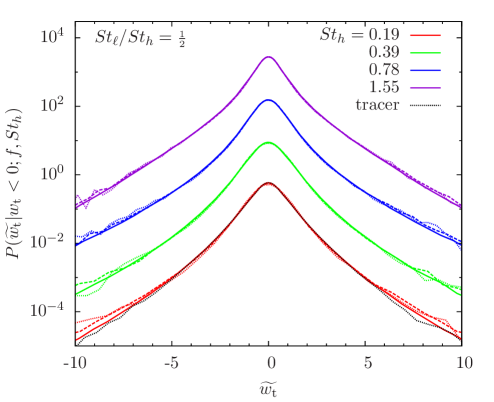
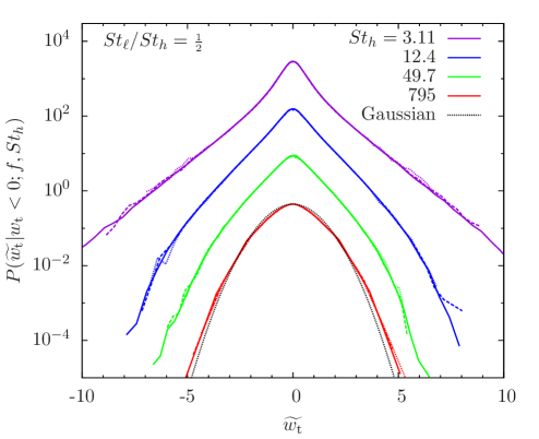
Figure 12.— The normalized PDF of the tangential relative velocity, $w_{\rm t}$, for approaching pairs with $f=\frac{1}{2}$ at $r=1$ (solid), $\frac{1}{2}$ (dashed) and $\frac{1}{4}\eta$ (dotted). For each PDF, $w_{\rm t}$ is normalized to its rms value, i.e., $\widetilde{w_{\rm t}}\equiv w_{\rm t}/\langle w_{\rm t}^{2}\rangle_{-}^{1/2}$. Left and right panels show $St_{h}\leq 0.78$ and $St_{h}\geq 1.55$, respectively. In both panels, the bottom lines show the actual PDF values, while upper lines for each larger (left panel) or smaller (right panel) $St_{h}$ are shifted upward by a factor of 16 for clarity. The black dotted lines in the left and right panels are the PDF of approaching tracer particles at $r=1\eta$ and the Gaussian fit for $St_{h}=795$, respectively.

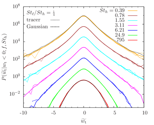
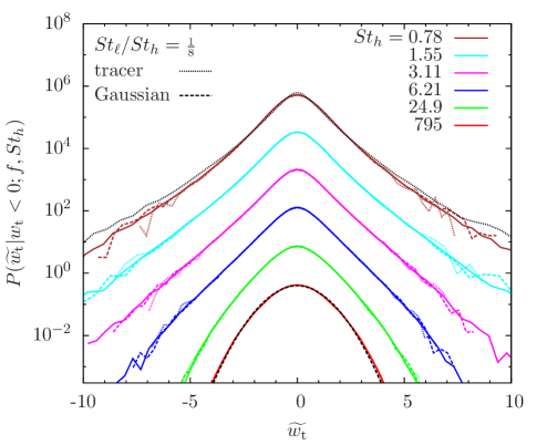
Figure 13.— The normalized tangential relative velocity PDF for approaching pairs with $f=\frac{1}{4}$ (left panel) and $f=\frac{1}{8}$ (right panel) at $r=1$ (solid), $\frac{1}{2}$ (dashed) and $\frac{1}{4}\eta$ (dotted). The bottom lines for $St_{h}=795$ show the actual values of the PDF, while the PDFs for each smaller $St_{h}$ is shifted upward by a factor of 16 for clarity. The black dotted and dashed lines in both panels are the PDF of tracer particles at $r=1\eta$ and the Gaussian fit for $St_{h}=795$, respectively.

At a given $f$ and $St_{h}$, the left and right tails of the radial PDF tend to be more symmetric as $r$ decreases. In particular, for $St_{h}=0.78$ and $1.55$ in both panels, the right tail slightly increases with decreasing $r$, while the left wing becomes narrower. The opposite trends of the two tails both reduce the negative skewness of the PDF. The increase in the right tail for these values of $St_{h}$ with decreasing $r$ is due to the shear contribution. The right wing corresponds to separating pairs, and, backward in time, the distance of these pairs first decreases in near past and then starts to increase as the two particles move past each other. At smaller $r$, it takes a shorter time for the distance of these pairs to switch from decreasing to increasing. Therefore, the primary distance, $r_{\rm p}$, of separating pairs at a friction time ago could increase with decreasing $r$, leading to a larger shear contribution and the increase in the right wing. On the other hand, for approaching pairs, $r_{\rm p}$ always tends to be smaller at smaller $r$, and the width of the left wing decreases with decreasing $r$. Overall, as $r$ decreases, the difference of $r_{\rm p}$ between approaching and separating pairs decreases, reducing the asymmetry of the two wings.

We attempted to check how the shape of the left wing for approaching particles changes with decreasing $r$ by normalizing the wing to its own rms. It turns out that, except for $f=\frac{1}{2}$ and $St_{h}=0.19$, the shape of the left wing is almost invariant with $r$, indicating that the $r-$dependence of the shape is weaker than that of the width or rms. The trend of the shape of the left wing with $f$ and $St_{h}$ is the same as the tangential PDF of approaching pairs, which we discuss in the next section.

4.2.3 The normalized PDF of the tangential relative velocity

In Fig. 12, we show the normalized PDF, $P(\widetilde{w_{\rm t}}|w_{\rm r}<0;f,St_{h})$, of the tangential relative speed for approaching particle pairs ($w_{\rm r}<0$) with a Stokes ratio of $f=\frac{1}{2}$. We normalized $w_{\rm t}$ to its rms value, i.e., $\widetilde{w_{\rm t}}\equiv w_{\rm t}/\langle w_{\rm t}^{2}\rangle_{-}^{1/2}$, where the subscript “-” indicates that only approaching pairs are counted. All the normalized PDFs have a unit variance. The normalization gives a clearer comparison of the PDF shape. The black dotted line in the left panel is the PDF of approaching tracer particles at $r=1\eta$, corresponding to $St_{h}=0$. As $St_{h}$ increases to $0.78$, the tails of $P(\widetilde{w_{\rm t}}|w_{\rm r}<0;f,St_{h})$ show a slow fattening trend. The fattening appears to be weak, but is verified by a computation of the kurtosis. Then, starting from $St_{h}=1.55$, the PDF shape becomes continuously thinner (the right panel). Similar to the monodisperse case, the PDF fatness peaks at $St_{h}\simeq 1$.

We tried to obtain a quantitative estimate of the PDF shape for $f=\frac{1}{2}$ by fitting the tails of $P(w_{\rm t}|w_{\rm r}\leq 0;f,St_{h})$ with stretched exponential functions (eq. (4)). We find that, as $St_{h}$ increases from 0.19, to 0.39 and 0.78, the best-fit value of $\alpha$ decreases from 0.7($r=1\eta$), to 0.67 and 0.6, indicating a slight tail fattening of the PDF. As $St_{h}$ increases further, $\alpha$ starts to increase. The best-fit $\alpha$ is 0.65, 0.8, 1.15, 1.33, 1.45, 1.55,1.65, 1.7, 1.75 and 1.9 for $St_{h}=1.55$, 3.11, 6.21, 12.4, 24.9, 49.7, 99.4, 199, 397 and 795, respectively. For $St_{h}=795$, the PDF is close to Gaussian (the black dotted line in the right panel), but the best-fit $\alpha$ is $1.9$, slightly smaller than 2. The measured $\alpha$ values also apply to the left wing of the radial PDF for $f=\frac{1}{2}$, which coincides with the left wing of $P(w_{\rm t}|w_{\rm r}<0;f,St_{h})$ (see §4.2.1). These values are generally larger than those obtained in Paper I for the monodisperse PDF with $St$ equal to $St_{h}$ listed here. This is due to the effect of the acceleration contribution which tends to make the PDF tails thinner.

To understand the trend of the PDF shape at $f=\frac{1}{2}$, we consider again the behavior of the generalized acceleration (${\boldsymbol{w}}_{\rm a}$) and shear (${\boldsymbol{w}}_{\rm s}$) contributions to the PDF. As discussed earlier, the PDF shape of ${\boldsymbol{w}}_{\rm a}$ would become thinner continuously with increasing $\tau_{\rm p,h}$ (see §3.1 and §4.1.1). Using the monodisperse case as a guideline for the generalized shear contribution, the distribution of ${\boldsymbol{w}}_{\rm s}$ would first fatten as $St_{h}$ increases toward 1, and then become thinner as the Stokes number increase further above 1. Therefore, at small $St_{h}\;\hbox to0.0pt{\lower 2.5pt\hbox{$\sim$}\hss}\raise 1.5pt\hbox{$<$}\;1$, the distributions of ${\boldsymbol{w}}_{\rm a}$ and ${\boldsymbol{w}}_{\rm s}$ have opposite trends with increasing $St_{h}$, and their competition determines the fatness of the relative velocity PDF. For $f=\frac{1}{2}$, it appears the fattening trend by ${\boldsymbol{w}}_{\rm s}$ wins, and the PDF of ${\boldsymbol{w}}$ becomes fatter as $St_{h}$ increases to $0.78$. Since the acceleration contribution tends to counteract the fattening trend, the increase of the tail fatness in the range $0.19\leq St_{h}\leq 0.78$ is significantly weaker than in the monodisperse case. As $St_{h}$ increases above 1, the PDF of ${\boldsymbol{w}}_{\rm s}$ starts the thinning trend, and, together with the thinning effect by the acceleration term, ${\boldsymbol{w}}_{\rm a}$, and the fatness of the PDF of ${\boldsymbol{w}}$ decreases, as observed in Fig. 12.

Fig. 13 plots the normalized tangential PDF for $f=\frac{1}{4}$ (left panel) and $f=\frac{1}{8}$ (right panel). In both panels, the black dotted line is the PDF for tracer particles ($St_{h}=0$) at $r=1\eta$, and the black dashed line is the Gaussian fit to $St_{h}=795$. For $f=\frac{1}{4}$, the minimum $St_{h}$ available in our simulation is $0.39$, and, for this $St_{h}$, the PDF shape is close to that of the tracers. It turns out that, for $f=\frac{1}{4}$, the PDF shape remains roughly unchanged as $St_{h}$ increases to $0.78$, and fitting the PDFs for $St_{h}\leq 0.78$ with stretched exponentials gives $\alpha=0.78$. This invariance of the PDF shape is probably due to the fact that the fattening effect of the shear term cancels out the thinning trend of the acceleration term in this range of $St_{h}$. For larger $St_{h}$ ($\;\hbox to0.0pt{\lower 2.5pt\hbox{$\sim$}\hss}\raise 1.5pt\hbox{$>$}\;1$), the PDF becomes thinner with increasing $St_{h}$, and the best-fit $\alpha$ increases from $\simeq 0.8$ at $St_{h}=1.55$ to 2 at $St_{h}\;\hbox to0.0pt{\lower 2.5pt\hbox{$\sim$}\hss}\raise 1.5pt\hbox{$>$}\;397$.

For $f=\frac{1}{8}$, the minimum $St_{h}$ we have is 0.78, and, as $St_{h}$ increases above 0.78, the PDF shape becomes continuously thinner (right panel). For $f=\frac{1}{8}$ and $St_{h}\;\hbox to0.0pt{\lower 2.5pt\hbox{$\sim$}\hss}\raise 1.5pt\hbox{$>$}\;0.78$, the acceleration term, ${\boldsymbol{w}}_{\rm a}$, dominates the contribution to the relative velocity, and the PDF of ${\boldsymbol{w}}_{\rm a}$ is thinner at larger $\tau_{\rm p,h}$.

From Fig. 12 and Fig. 13, we see that the PDF shape is almost independent of $r$. Except for $f=\frac{1}{2}$ and $St_{h}=0.19$, the shape of all the PDFs in these figures already converges at $r\simeq\frac{1}{2}\eta$. The $r-$dependence of the PDF shape is much weaker than the monodisperse case, and the dependence decreases with decreasing $f$. As explained before, this is due to the acceleration contribution in the bidisperse case, which is independent of $r$. In the case with $f=\frac{1}{2}$ and $St_{h}=0.19$, corresponding to the two smallest particles in our simulation, the PDF tails become slightly fatter with decreasing $r$. For this Stokes pair, the relative velocity at $r\;\hbox to0.0pt{\lower 2.5pt\hbox{$\sim$}\hss}\raise 1.5pt\hbox{$>$}\;\frac{1}{4}\eta$ still has a significant $r-$dependent shear contribution. To achieve convergence for this case, a resolution below $r\;\hbox to0.0pt{\lower 2.5pt\hbox{$\sim$}\hss}\raise 1.5pt\hbox{$<$}\;\frac{1}{4}\eta$ is needed.

In Appendix C, we compare the tangential PDFs for approaching and separating pairs, which is of theoretical interest. We show that, because the generalized acceleration term is independent of the relative motions of the two particles, the difference between the PDFs of approaching and separating pairs decreases when ${\boldsymbol{w}}_{\rm a}$ increases with decreasing $f$.

4.2.4 The PDF of the 3D amplitude

In Fig. 14, we show the normalized PDF, $P(\widetilde{|{\boldsymbol{w}}}||w_{\rm r}<0;f,St_{h})$, of the 3D amplitude, $|{\boldsymbol{w}}|$, of the relative velocity for approaching particle pairs with a Stokes ratio $f=\frac{1}{2}$. For each PDF, we normalized $|{\boldsymbol{w}}|$ to its rms, $\langle w^{2}\rangle_{-}^{1/2}$. The figure is plot in a similar way as Fig. 14 of Paper I. But unlike that figure, which shows the PDF only at one distance ($r=1\eta$), here we plot the results for $r=1\eta$ and $\frac{1}{2}\eta$. In the left panel, we see that, as $St_{h}$ increases from $0.19$ (red) to 1.55 (blue), the PDF around the rms value (i.e., $\widetilde{|{\boldsymbol{w}}|}\simeq 1$) slightly decreases, and more probabilities are transferred to the left and right parts of the PDF at $\widetilde{|{\boldsymbol{w}}|}\ll 1$ and $\widetilde{|{\boldsymbol{w}}|}\gg 1$, respectively. This trend corresponds to the fattening of the PDFs of the radial and tangential relative speeds with increasing $St_{h}$ at small $St_{h}$ (see Fig. 12 and discussions in §4.2.3). Note that the far right PDF tail for $St_{h}=1.55$ already becomes thinner than that for $St_{h}=0.78$, consistent with the observation in Fig. 12 that the thinning of the tangential PDF tails starts at $St_{h}\;\hbox to0.0pt{\lower 2.5pt\hbox{$\sim$}\hss}\raise 1.5pt\hbox{$>$}\;0.78$.

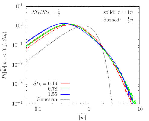
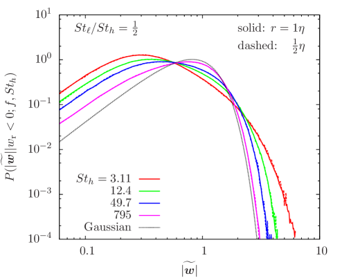
Figure 14.— The PDF of the 3D relative velocity amplitude for approaching particle pairs at $r=1\eta$ (solid) and $\frac{1}{2}\eta$ (dashed). The Stokes ratio is fixed at $f=\frac{1}{2}$. The 3D amplitude, $|{\boldsymbol{w}}|$, is normalized to the rms value, i.e., $\widetilde{|{\boldsymbol{w}}|}=|{\boldsymbol{w}}|/\langle w^{2}\rangle_{-}^{1/2}$, so that each PDF in the figure has unit variance. The left and right panels show $St_{h}\leq 1.55$ and $St_{h}\geq 3.11$, respectively. In both panels, the black dotted line is the normalized PDF of the amplitude of a 3D Gaussian vector.

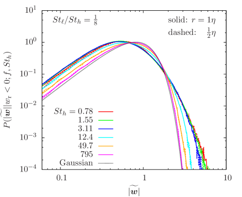
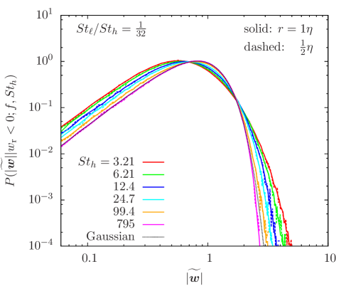
Figure 15.— The normalized 3D relative velocity PDFs for $f=\frac{1}{8}$ (left) and $f=\frac{1}{32}$ (right). The solid and dashed lines correspond to $r=1$ and $\frac{1}{2}\eta$, respectively. The black dotted line is the normalized PDF for the amplitude of a 3D Gaussian vector.

For $St_{h}$ above 3.11, the PDF shape has an opposite trend. With increasing $St_{h}$, the probability is more concentrated around the rms value, and the PDF at very small and large relative velocities decreases, as expected from the thinning of the radial and tangential PDFs for $St_{h}$ in this range. In the limit $St_{h}\to\infty$, the PDF is expected to approach Gaussian (black dotted line), but for the largest $St_{h}$ ($=795$) in the simulation, the PDF is still slightly non-Gaussian, especially at $\widetilde{|{\boldsymbol{w}}|}\ll 1$. The general trend of the 3D amplitude PDF for $f=\frac{1}{2}$ as a function of $St_{h}$ is similar to the monodisperse case shown in Fig. 14 of Paper I. Comparing with that figure, we see again that the PDF tails in the bidisperse case are significantly less fat than for equal-size particles.

The left panel Fig. 15 shows the normalized PDF of the 3D amplitude for $f=\frac{1}{8}$. The minimum $St_{h}$ available is $0.78$, and, consistent with the early results (see the right panel of Fig. 13) for the tangential PDF, the right tail of $P(\widetilde{|{\boldsymbol{w}}|}|w_{\rm r}<0;f,St_{h})$ at large $\widetilde{|{\boldsymbol{w}}|}$ keeps thinning for all $St_{h}\geq 0.78$. The PDF becomes close to Gaussian (dotted black line) for $St_{h}\;\hbox to0.0pt{\lower 2.5pt\hbox{$\sim$}\hss}\raise 1.5pt\hbox{$>$}\;199$. The PDF for $f=\frac{1}{32}$ in the right panel has the same trend.

Although the bidispserse PDF is thinner than the case of equal-size particles, significant non-Gaussianity still exists, especially if both particles are small. The PDF is close to Gaussian only if one or both particles are sufficiently large. It is of practical interest to examine the particle size range in which the relative velocity PDF can be approximated by Gaussian. For a given $St_{h}$ or $\tau_{\rm ph}$, the PDF becomes thinner and closer to Gaussian as $f$ decreases. Interestingly, we find that, for a fixed $\tau_{\rm ph}$, the shape of the PDF barely changes as $f$ decreases from $\frac{1}{16}$ to 0. The reason is that, for $f$ in this range, the particle relative velocity, ${\boldsymbol{w}}$, is dominated by the generalized acceleration term, whose distribution is controlled by $\Delta{\boldsymbol{u}}_{\rm T}(\tau_{\rm ph})$. In the $f\to 0$ ($St_{\ell}\to 0$) limit, ${\boldsymbol{w}}$ approaches the particle-flow relative velocity, ${\boldsymbol{w}}_{\rm f}$, and, based on our results in §3.1, the PDF of ${\boldsymbol{w}}_{\rm f}$ is close to Gaussian if the particle friction time is larger than $3.5T_{\rm L}$. It follows that, for any $f$ in the range $0\leq f\leq\frac{1}{16}$, the particle relative velocity PDF is approximately Gaussian if $\tau_{\rm ph}\;\hbox to0.0pt{\lower 2.5pt\hbox{$\sim$}\hss}\raise 1.5pt\hbox{$>$}\;3.5T_{\rm L}$ (corresponding to $St_{h}\;\hbox to0.0pt{\lower 2.5pt\hbox{$\sim$}\hss}\raise 1.5pt\hbox{$>$}\;49.7$ in our flow). The condition for the relative velocity PDF to have a Gaussian shape is stronger for $\frac{1}{16}<f\leq 1$. For example, at $f=\frac{1}{8}$ and $f=\frac{1}{4}$, Gaussianity is reached only for $\tau_{\rm ph}\;\hbox to0.0pt{\lower 2.5pt\hbox{$\sim$}\hss}\raise 1.5pt\hbox{$>$}\;14T_{\rm L}$ and $\tau_{\rm ph}\;\hbox to0.0pt{\lower 2.5pt\hbox{$\sim$}\hss}\raise 1.5pt\hbox{$>$}\;27T_{\rm L}$, respectively. For $f=\frac{1}{2}$ (Fig. 14) and $f=1$ (Fig. 14 of paper I), the PDF still shows some (slight) degree of non-Gaussianity even for the largest particles ($\tau_{\rm ph}=54T_{\rm L}$) in our simulation.

In Figs.  14 and 15, we see that the shape of the normalized PDF for the 3D amplitude already converges at $r=\frac{1}{2}\eta$, except for the relative velocity between the two smallest particles in our simulation (the red lines in the left panel of Fig. 14). The convergence is also found for other $f$ values not shown here. The $r-$dependence of the relative velocity PDF is stronger in the monodisperse case, and it does not converge at $r\simeq 1\eta$ for equal-size particles with $St\;\hbox to0.0pt{\lower 2.5pt\hbox{$\sim$}\hss}\raise 1.5pt\hbox{$<$}\;3.11$ (see Fig. 6). In the bidisperse case, the generalized acceleration contribution is independent of $r$ (§2) and its presence helps reduce the $r-$dependence of the relative velocity statistics. This finding is of particular interest for applications to dust particle collisions in protoplanetary disks. Dust particles should be viewed as nearly-point particles (e.g., Hubbard 2012), and one needs to examine the collision velocity PDF in the $r\to 0$ limit. The weaker $r-$dependence of the bidisperse PDF makes it easier to resolve the relative velocity or collision statistics at $r\to 0$.

In comparison to a Gaussian distribution, the PDFs measured in our simulation have more probabilities at both extremely small and large collision speeds. Clearly, the fat high tails of the PDF may lead to significantly higher probability of fragmentation than predicted under the Gaussian assumption (Windmark et al. 2012b, Garaud et al. 2013). On the other hand, the PDF at low collision velocity is also considerably higher than a Gaussian distribution, which would favor sticking of the particles. The competition of these two effects is important for understanding how the non-Gaussianity of the collision velocity affects the growth of dust particles in protoplanetary disks. In next section, we give some speculations using our simulation results, but a definite answer requires evolving the particle size distribution with a coagulation model that accounts for the non-Gaussian collision velocity.

5. Implications of Non-Gaussianity on Dust Particle Collisons

5.1. Parameters and Assumptions

We discuss the effect of the non-Gaussianity of turbulence-induced collision velocity on dust particle collisions in protoplanetary disks. Using the probability distribution measured in our simulation, we will roughly estimate the fractions of collisions leading to sticking, bouncing and fragmentation, as the particle size grows. We adopt a minimum mass solar nebula. The profiles of the gas density, sound speed and scale height are set to $\rho=1.7\times 10^{-9}(R/{\rm AU})^{-2.75}$ g cm^-3, $C_{\rm s}=1.0(R/{\rm AU})^{-0.25}$ km s^-1, and $H=5\times 10^{6}(R/{\rm AU})^{1.25}$ km, with $R$ the distance to the central star. As our main purpose is to give a simple illustrating example, we primarily consider $R=1$ AU. At 1AU, the mean free path, $\lambda$, of the gas is $\simeq 1$ cm, and, using the Epstein and Stokes formulae, we find the friction time $\tau_{\rm p}=6\times 10^{3}(a_{\rm p}/{\rm cm})$ s and $\tau_{\rm p}=2.3\times 10^{3}(a_{\rm p}/{\rm cm})^{2}$ s for particle size, $a_{\rm p}$, below and above $\lambda$, respectively. The two formulae connect at $a_{\rm p}\simeq 2.6$ cm.

We use the prescription of Cuzzi et al. (2001) to specify turbulence conditions in protoplanetary disks with the Shakura-Sunyaev parameter $\alpha_{\rm t}$. The large-eddy turnover time is set to $T_{\rm eddy}=\Omega_{\rm K}^{-1}=5\times 10^{6}(R/{\rm AU})^{3/2}$ s with $\Omega_{\rm K}$ the Keplerian rotation frequency. The turbulent rms velocity and integral scale are given by $U=\alpha_{\rm t}^{1/2}C_{\rm s}$ and $L=\alpha_{\rm t}^{1/2}H$, respectively. Note that here $U$ is the 3D rms velocity, different from $u^{\prime}$ given earlier for the 1D rms of our simulated flow. Taking a fiducial value of $10^{-4}$ for $\alpha_{\rm t}$, we have $U=10(\alpha_{\rm t}/10^{-4})^{1/2}$ m s^-1, and $L=5\times 10^{4}(\alpha_{\rm t}/10^{-4})^{1/2}$ km at 1AU. Adopting a dynamical viscosity of $9\times 10^{-5}$ g cm^-1 s^-1 for molecular hydrogen at $\simeq$ 300 K, the Reynolds number is estimated to be $Re\simeq 10^{8}(\alpha_{\rm t}/10^{-4})$. The Kolmogorov time and length scales are given by $\tau_{\eta}\simeq T_{\rm eddy}Re^{-1/2}=500(\alpha_{\rm t}/10^{-4})^{-1/2}$ s, and $\eta\simeq LRe^{-3/4}=0.05(\alpha_{\rm t}/10^{-4})^{-1/4}$ km. At 1AU, particles of mm size have $\tau_{\rm p}\simeq\tau_{\eta}$ or $St\simeq 1$. We also define a Stokes number based on the large-eddy time as $St_{\rm eddy}\equiv\tau_{\rm p}/T_{\rm eddy}$, and, at 1AU, $St_{\rm eddy}\simeq 1$ corresponds to $a_{\rm p}\simeq 50$ cm.

The collision outcome for particles over a wide size range is complicated, and its dependence on the collision velocity and the particle internal structure is subject of ongoing investigations. A summary of experimental results is given by Güttler et al. (2010). Here we adopt the assumption of Windmark et al. (2012b) and Garaud et al.  (2013) to determine the collision outcome of silicate particles. Particles are assumed to stick if the 3D amplitude of the collision velocity, $|\boldsymbol{w}|$, is below a bouncing threshold $w_{\rm b}$ of 5 cm s^-1, while fragmentation takes place for $|\boldsymbol{w}|$ above a threshold $w_{\rm f}\simeq 1$ m s^-1. Between $w_{\rm b}$ and $w_{\rm f}$, the colliding particles bounce off each other. Following Garaud et al.  (2013), we compute the fractions of sticking, bouncing and fragmentation as $F_{\rm s}=\int_{0}^{w_{\rm b}}|\boldsymbol{w}|P(|\boldsymbol{w}|;f,St_{h})d|\boldsymbol{w}|/\langle|\boldsymbol{w}|\rangle$, $F_{\rm b}=\int_{w_{\rm b}}^{w_{\rm f}}|\boldsymbol{w}|P(|\boldsymbol{w}|;f,St_{h})d|\boldsymbol{w}|/\langle|\boldsymbol{w}|\rangle$, and $F_{\rm f}=\int_{w_{\rm f}}^{\infty}|\boldsymbol{w}|P(|{\boldsymbol{w}}|;f,St_{h})d|\boldsymbol{w}|/\langle|\boldsymbol{w}|\rangle$, respectively, where $P(|\boldsymbol{w}|;f,St_{h})$ is the PDF of $|\boldsymbol{w}|$, and $\langle|\boldsymbol{w}|\rangle\equiv\int_{0}^{\infty}|\boldsymbol{w}|P(|\boldsymbol{w}|;f,St_{h})d|\boldsymbol{w}|$ is the mean of $|\boldsymbol{w}|$. Unlike the fractions defined in Windmark et al. (2012b), a weighting factor $\propto|\boldsymbol{w}|$ is included in these equations, accounting for higher collision frequency for particle pairs with larger relative velocity (Garaud et al.  2013). The weighting factor used here is based on the cylindrical formulation of the collision kernel, where the collision rate $\propto|\boldsymbol{w}|$ (see Paper I).

In our calculation, we adopt PDFs measured at $r=\frac{1}{2}\eta$. It is desirable to use PDFs at smaller $r$ because the relative velocity statistics of small particles ($St\;\hbox to0.0pt{\lower 2.5pt\hbox{$\sim$}\hss}\raise 1.5pt\hbox{$<$}\;1$) of similar sizes ($f=1$ or $\frac{1}{2}$) have not converged at $r=\frac{1}{2}\eta$. However, the measured PDFs at smaller $r$($\leq\frac{1}{4}\eta$) are very noisy because the number of particle pairs available in our simulation becomes too limited at $r\leq\frac{1}{4}\eta$. The choice of using the PDF data at $r=\frac{1}{2}\eta$ is sufficient for an illustration purpose, especially as we are more concerned with the collisions of inertial-range particles with $St$ considerably above 1 (corresponding to $a_{\rm p}\gg 1$ mm at 1AU). The PDFs for these relatively large particles already converge at $r=\frac{1}{2}\eta$. For small, similar-size particles, our estimates for the fractions need to be improved by future simulations that can accurately measure the PDFs at smaller $r$.

The inertial range of our simulated flow is short, and one needs to be careful when applying the measured statistics to protoplanetary turbulence. Since the realistic $Re(\simeq 10^{8})$ in the disk cannot be reached by currently available computation power, the best solution is to extrapolate the simulation results to high $Re$. The extrapolation requires the $Re-$dependence of the PDF, which is currently unknown. We are thus forced to use rather strong assumptions. For a clear description of our assumptions, we distinguish the Stokes numbers in our simulated flow and in the real disk. We use $St^{\rm s}$ and $St_{\rm eddy}^{\rm s}$ to denote the Stokes numbers based on $\tau_{\eta}$ and $T_{\rm eddy}$ in our simulation, while $St^{\rm d}$ and $St_{\rm eddy}^{\rm d}$ are the corresponding numbers in the disk. In our flow, $T_{\rm eddy}\simeq 20\tau_{\eta}$ and thus $St^{\rm s}\simeq 20St_{\rm eddy}^{\rm s}$. Due to a much broader inertial range in the disk, we have $St^{\rm d}\simeq 10^{4}St_{\rm eddy}^{\rm d}$ at 1AU.

The only species of particles that definitely lie in the inertial range of our simulated flow are those with $St^{\rm s}=6.21$ (or equivalently $St_{\rm eddy}^{\rm s}=0.31$). Larger particles with $St^{\rm s}\geq 12.4$ ($St_{\rm eddy}^{\rm s}\geq 0.62$) and smaller ones with $St^{\rm s}\leq 3.11$ ($St^{\rm s}_{\rm eddy}\leq 0.16$) are affected by the flow structures at driving and dissipation scales, respectively. Accordingly, we divide dust particles in the disk into three ranges, i.e, the driving range with $St_{\rm eddy}^{\rm d}\geq 0.62$ ($St^{\rm d}\geq 6.2\times 10^{3}$), the dissipation range with $St^{\rm d}\leq 3.11$ ($St_{\rm eddy}^{\rm d}\leq 3.1\times 10^{-4}$), and the inertial range with $3.11\times 10^{-4}<St_{\rm eddy}^{\rm d}<0.62$ ($3.11<St^{\rm d}<6.2\times 10^{3}$). Our measurement for $St_{\rm eddy}^{\rm s}\geq 0.62$ particles can be directly applied to corresponding particles with $St_{\rm eddy}^{\rm d}\geq 0.62$ in the disk because collisions of these particles are determined by large-scale structures that are resolved in our simulation. For particles in the inertial range, we make a strong simplification. We use the PDF shape of the only inertial-range particle ($St^{\rm s}_{\rm eddy}=0.31$) in our flow for all inertial-range particles ($3.11\times 10^{-4}<St_{\rm eddy}^{\rm d}<0.62$) at 1AU in the disk. Finally, for dissipation-range particles with $St^{\rm d}\leq 3.11$ in the disk, we assume the PDF shape at each $St^{\rm d}$ is the same as the PDF of particles with $St^{\rm s}=St^{\rm d}$ in our flow.

For the rms width of the PDF, we make use of the prediction of the PP10 model (Papers I & II) with a Reynolds number ($Re\simeq 10^{8}$) appropriate for the disk. In particular, the model predicts a $(St^{\rm d})^{1/2}$ scaling for equal-size particles in the inertial range ($3.11<St^{\rm d}<6.2\times 10^{3}$). Similar approximations are used for different particles with a fixed Stokes ratio, $f\equiv{St_{\ell}}/St_{h}$. We divide particle pairs at a given $f$ into the same three ranges based on the Stokes number, $St_{h}^{\rm d}$ (or $St_{{\rm eddy},h}^{\rm d}$), of the larger particle. We then take the same procedure for the PDF shape as a function of $St_{h}^{\rm d}$ using the simulation data for the three ranges. Again, the rms relative velocity at fixed $f$ is taken from our model, which predicts a $(St_{h}^{\rm d})^{1/2}$ scaling for $St_{h}^{\rm d}$ in the inertial range for any value of $f$.

5.2. Fractions of Sticking, Bouncing and Fragmentation

Fig. 16 shows the fractions of sticking, bouncing and fragmentation as a function of the size of the larger particle, $a_{\rm p,h}$, at different Stokes ratios, $f$. Each panel is plot in a similar way as Fig. 1 in Windmark et al. (2012b). As the particles grow, the collision velocity increases, and bouncing and finally fragmentation take place. The vertical brown and black dotted lines correspond to particle sizes, at which the rms collision velocities, $\langle w^{2}\rangle^{1/2}$ , become equal to the bouncing ($w_{\rm b}$) and fragmentation ($w_{\rm f}$) thresholds. If we ignore the collision velocity distribution and assume that, for each size pair, the collision velocity is single-valued with $P(|\boldsymbol{w}|;f,St_{h})=\delta(|\boldsymbol{w}|-\langle w^{2}\rangle^{1/2})$, these vertical lines mark instantaneous transitions to bouncing and fragmentation, which occur typically at millimeter and decimeter sizes, respectively. In this case, the growth would stop once the size reaches the brown line, a problem known as the bouncing barrier for planetesimal formation. If the particle growth somehow manages to pass the bouncing barrier, it would eventually be frustrated by the fragmentation barrier (black dotted line). As $f$ decreases from 1 (top panel) toward 0 (bottom panel), the vertical lines shift toward smaller sizes because the rms relative velocity increases with decreasing $f$ (see Fig. 7 in Paper II).

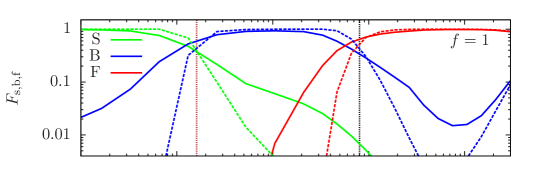
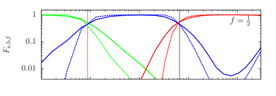
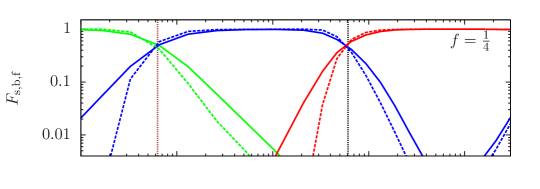
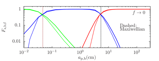
Figure 16.— Sticking (green), bouncing (blue) and fragmentation (red) fractions as a function of the size, $a_{\rm{p,h}}$, of the larger particle. The four panels show fixed Stokes number ratios at $f=1$, $\frac{1}{2}$, $\frac{1}{4}$, and $f\to 0$. Vertical brown and black dotted lines correspond to critical $a_{\rm{p,h}}$ at which the rms relative velocity reaches bouncing and fragmentation thresholds, respectively. Dashed lines assume a Maxwellian distribution. Results for $f\to 0$ are based on the particle-flow relative velocity (§3.1).

Assuming a Maxwellian distribution for $|\boldsymbol{w}|$, Windmark et al. (2012b) and Garaud et al. (2013) examined the effect of the collision velocity PDF on particle growth. As shown in Fig. 1 of Windmark et al. (2012b), accounting for the PDF leads to gradual transitions from sticking to bouncing and to fragmentation. The reason is clear: With a probability distribution, there are always possibilities for sticking (or bouncing), corresponding to the low (or high) tail of the $|\boldsymbol{w}|$ PDF, even if the rms collision velocity is already above (or still below) the bouncing threshold, $w_{\rm b}$. The same applies to the bouncing-to-fragmentation transition. For comparison with the estimates based on our simulation data, the dashed lines in Fig. 16 show the fractions computed from a Maxwellian PDF for $|\boldsymbol{w}|$ using the PP10 model prediction for the rms width. An interesting result of Windmark et al. (2012b) was that, accounting for the $|\boldsymbol{w}|$ distribution, the bouncing barrier may be overcome. The sticking probability beyond the barrier size allows further growth, and the peak of the particle size distribution, $p(a_{\rm p})$, can move past the vertical brown line. Intuitively, a large particle can from if, by “luck”, it kept encountering sticking events and enjoyed continuous growth.

The transition from bouncing to fragmentation is also gradual, and of particular interest is the finite probability of fragmentation before $a_{\rm p}$ reaches the black dotted line, corresponding to the high tail of the PDF of $|{\boldsymbol{w}}|$. These fragmentation events would replenish particles of small sizes, increasing the size distribution, $p(a_{\rm p})$, at small $a_{\rm p}$ (Windmark et al. 2012b). Under the assumption of a Maxwellian PDF, the decrease of the sticking probability is rather fast (the green dashed lines), and the growth past the bouncing barrier turns out to be slow. Windmark et al. (2012b) showed that it takes $\sim 10^{4}$ yr to reach centimeter size. The growth by sticking toward the fragmentation barrier (if not impossible) would take significantly longer than $10^{4}$ yr. Note that, after the bouncing-to-fragmentation transition, the bouncing fraction (blue lines) in the top three panels start to increase at $a_{\rm p,h}\simeq 0.5-1$ m. The reason is that the rms relative velocity for a given Stokes ratio $f$ starts to decrease at $\tau_{\rm p,h}/T_{\rm eddy}\;\hbox to0.0pt{\lower 2.5pt\hbox{$\sim$}\hss}\raise 1.5pt\hbox{$>$}\;1/f$ (see Fig. 7 of paper II).

The solid lines in Fig. 16 are the fractions based on our simulation data for the collision velocity PDF. These lines show more gradual transitions than the dashed ones for a Maxwellian distribution. This is because the collision PDF measured in our flow is fatter than a Gaussian distribution. As mentioned earlier, in our terminology a fat PDF shape typically corresponds to a sharper inner part and a fatter tail part. In Figures 14 and 15, we see that the measured PDFs have higher probabilities at both extremely small and large $|{\boldsymbol{w}}|$ than a Maxwellian distribution. Consider, for example, the switch from sticking to bouncing. The higher probability at small $|{\boldsymbol{w}}|$ is responsible for the slower decrease of $F_{\rm s}$ with the size of the larger particle, while the earlier rise of the bouncing curves, $F_{\rm b}$, at smaller $a_{\rm p,h}$ is due to higher probability of large $|{\boldsymbol{w}}|$ at the right tail.

Interestingly, in the top panel for equal-size particles, the decrease of $F_{\rm s}$ past the bouncing barrier is quite slow, and it even extends to the fragmentation barrier (black dotted line). This can be understood from Fig. 14 in Paper I for equal-size particles, which shows that the PDF at extremely small $|{\boldsymbol{w}}|$ is orders of magnitude larger than a Gaussian distribution. An immediate implication of the persistence of significant sticking fraction is that it further helps alleviate the problem of the bouncing barrier. With significantly higher sticking probabilities, the growth beyond the bouncing barrier would proceed faster than predicted with a Maxwellian distribution. The peak size of the distribution $p(a_{\rm p})$ would increase faster. In the $f=1$ and $\frac{1}{2}$ cases (top two panels), accounting for non-Gaussianity may accelerate the growth by a factor of $\;\hbox to0.0pt{\lower 2.5pt\hbox{$\sim$}\hss}\raise 1.5pt\hbox{$>$}\;10$.

Due to the fat non-Gaussian PDF tail, the solid red lines for fragmentation rise earlier than the dashed ones, suggesting that fragmentation can occur at smaller sizes and at a higher rate. One consequence is that it provides faster replenishment of smaller particles than the Maxwellian case, increasing the size distribution $p(a_{\rm p})$ at small $a_{\rm p}$. Together with the significantly higher sticking fraction, we speculate that this would lead to a broader size distribution $p(a_{\rm p})$ around the peak size. Another consequence of the earlier start of fragmentation is that it may begin to impede the growth at smaller sizes. As the peak of $p(a_{\rm p})$ moves closer to the fragmentation barrier, coagulational growth will finally end at a size where the fragmentation fraction, $F_{\rm f}$, exceeds the sticking fraction, $F_{\rm s}$. We see in Fig. 16 that the solid green and red lines tend to cross at smaller particle sizes than the dashed lines, meaning that, with non-Gaussian PDFs, fragmentation may start to compete with sticking earlier than the Maxwellian case. However, we argue this is a secondary effect in comparison to much higher sticking/growth rate between the bouncing and fragmentation barriers. We expect that the non-Gaussianity effect makes the growth toward the fragmentation barrier size considerably easier. Once the fragmentation fraction dominate over sticking, the possibility of further growth of some particles toward or above the fragmentation barrier requires alternative mechanisms, such as the sweep-up process discussed below.

As $f$ decreases from 1 toward 0, the solid lines becomes closer to the dashed ones. This is consistent with our results in §4.2 that, at a given $St_{h}$, the PDF shape becomes thinner with decreasing $f$. In particular, the degree of non-Gaussianity decreases very rapidly as $f$ goes from 1 to $\frac{1}{2}$, as can be seen by comparing Fig. 14 of Paper I and Fig. 14 in §4.2.4. The effect of non-Gaussianity is thus weaker for collisions between particles of very different sizes. The faster particle growth due to the effect of non-Gaussianity in between the bouncing and fragmentation barriers may occur mainly for particles of similar sizes.

The bottom panel for $f\to 0$ in Fig. 16 corresponds to particles of very different sizes. The computation is based on the particle-flow relative velocity discussed in §3.1. As the collision statistics change only slightly as $f$ decreases from $\frac{1}{16}$ to 0, this panel can be approximately used for any $f$ in the range $0\leq f\;\hbox to0.0pt{\lower 2.5pt\hbox{$\sim$}\hss}\raise 1.5pt\hbox{$<$}\;\frac{1}{16}$. The $f\to 0$ case is imporant for a particle growth mechanism called the mass transfer by fragmentation (see Windmark et al. 2012a). Laboratory experiments showed that, when colliding with a much larger particle, a small particle may break up and leave some fragments on the larger particle. In effect, the larger particle sweeps up masses from small particles, and it can thus keep growing even if its size already exceeds the fragmentation barrier size. The sweep-up mechanism was suggested as a possible path to planetesimal formation (Windmark et al. 2012a, 2012b; Garaud et al. 2013). The solid red line in the bottom panel can be viewed as representing the probability of such mass transfer or sweep-up events. In comparison to the Maxwellian case, the mass transfer can start earlier, suggesting that the sweep-up mechanism can operate at smaller $a_{\rm p,h}$.

We argue that, when the non-Gaussian collision statistics is included, the sweep-up growth is likely more efficient than the Maxwellian case because a larger number of seed particles of large sizes would be available to sweep up small particles. As discussed above, the formation of these particles is expected to be easier due to larger sticking probability in between the bouncing and fragmentation barriers. Also, the earlier start and higher rate of fragmentation from collisions of similar-size particles between the two barriers could help provide more small particles for the seed particles to sweep up. However, we emphasize these are only speculations, and a definite answer requires including the non-Gaussian PDFs into a coagulation model.

5.3. Discussions

We have shown that the non-Gaussianity of the collision velocity leads to more gradual transitions from sticking to bouncing and to fragmentation. The probability of sticking past the mean bouncing barrier is significantly larger than expected from a Maxwell distribution, and we argued this would further help alleviate the bouncing barrier, and help provide seed particles for the sweep-up process in a possible mechanism for planetesimal formation.

We point out that our assumption for the PDF of $|{\boldsymbol{w}}|$ underestimates the degree of non-Gaussianity for particles with $St_{\rm eddy}^{\rm d}\;\hbox to0.0pt{\lower 2.5pt\hbox{$\sim$}\hss}\raise 1.5pt\hbox{$<$}\;0.31$ ($a_{\rm p}\;\hbox to0.0pt{\lower 2.5pt\hbox{$\sim$}\hss}\raise 1.5pt\hbox{$<$}\;26$ cm) in the disk. As discussed in §2, the relative velocity of smaller particles samples the flow velocity at smaller scales, $\ell$. As the flow structures are more intermittent at smaller $\ell$, the PDF of $|{\boldsymbol{w}}|$ would become fatter as $St_{\rm eddy}^{\rm d}$ decreases. Thus, using the PDF shape of $St_{\rm eddy}^{\rm s}=0.31$ particles in our flow for all inertial-range particles in the disk underestimates the non-Gaussianity at $St_{\rm eddy}^{\rm d}<0.31$. The PDF for particles in the dissipation range ($St^{\rm d}\;\hbox to0.0pt{\lower 2.5pt\hbox{$\sim$}\hss}\raise 1.5pt\hbox{$<$}\;1$) of the disk would also be fatter than the corresponding particles ($St^{\rm s}\;\hbox to0.0pt{\lower 2.5pt\hbox{$\sim$}\hss}\raise 1.5pt\hbox{$<$}\;1$) in our flow, because the degree of turbulent intermittency at dissipation-range scales increases with $Re$. Therefore, the non-Gaussianity effects discussed above on the particle growth should be viewed as a lower limit. With more accurate PDF shape at $St_{\rm eddy}^{\rm d}\;\hbox to0.0pt{\lower 2.5pt\hbox{$\sim$}\hss}\raise 1.5pt\hbox{$<$}\;0.31$, the transitions to bouncing and fragmentation would appear to be more gradual. In a future work, we will examine the $Re-$dependence of the collision statistics using a $1024^{3}$ simulation, extrapolate the measured PDFs to large $Re$, and provide fitting functions that can be implemented in coagulation models.

We finally discuss some caveats in our results. Unlike our simulated flow, turbulence in a rotating disk is anisotropic at large scales. For example, in magneto-rotational disks, nearly axisymmetric structures, known as zonal flows (e.g., Johansen et al. 2009), emerge. Turbulent structures at large scales are highly elongated in the azimuthal (or zonal) direction. Based on Kolmogorov’s similarity hypothesis (e.g., Monin & Yaglom 1975), we expect the statistical isotropy to be restored at small scales where the eddy time is significantly smaller than the rotation period. Therefore, our results for the collision velocity PDF are applicable for small particles that couple to eddies far below the large zonal structures.

On the other hand, large particles with friction time, $\tau_{\rm p}$, near or above the rotation period, $\Omega_{\rm K}^{-1}$, would be affected by the anisotropic zonal flow, where azimuthal turbulent motions are more intense than in the radial direction. Stronger zonal structures indicate that the particle collision velocity primarily lies in the azimuthal direction, and the separation of nearby particle pairs backward in time would also proceed mainly in that direction. From the PP10 picture, the relative velocity of these large particles would mainly sample the flow structures in the zonal direction. Therefore, to understand the collision velocity PDF, we need to know the scaling behavior and the probability distribution of the zonal turbulent structures as a function of length and time scales, which, to our knowledge, are currently unavailable in the literature. It is thus unclear how the anisotropy in a rotating disk exactly affects the collision velocity PDF for particles with $\tau_{\rm p}$ close to $\Omega_{\rm K}^{-1}$. A direct comparison of the PDFs measured in our flow with simulation results for rotating disks in future studies would help reveal the effects of large-scale zonal flows on the particle collision statistics.

In addition to its effects on the flow structures, rotation could also directly affect the particle collision velocity. For example, the rotation velocities of particles of different sizes are different, and this gives rise to a mean azimuthal collision velocity, which may be important for very large particles (e.g., Fig. 3 of Testi et al. 2014). Differential rotation (or shear) can also contribute to the collision velocity. Although weaker than the zonal eddies, turbulent motions in the radial direction can cause a radial separation of nearby particle pairs backward in time. The particle pair would thus have a memory of different rotation speeds of the gas at different radii in the past, leading to a contribution to the collision velocity in the azimuthal direction. Combined with the radial separation, the differential rotation can enhance the backward separation of particle pairs in the azimuthal direction. This also tends to increase the collision velocity, as the particles’ memory would sample the zonal turbulent structures at large scales. The strength of these effects depends on the amplitude of the radial turbulent motions and thus on the degree of anisotropy. A definite estimate for the effects is beyond the scope of this work.

6. Summary and Conclusions

Motivated by the important role of the collision velocity distribution in modeling dust particle growth, we investigated the probability distribution function of turbulence-induced relative velocity of inertial particles, extending our earlier work on equal-size particles (Pan & Padoan 2013; Paper I) to the case of different particles of arbitrary sizes. We used the numerical simulation of Paper I. The simulation evolved inertial particles with friction time, $\tau_{\rm p}$, ranging from $0.1\tau_{\eta}$ ($St=0.1$) to $54T_{\rm L}$ ($St=795$), with $\tau_{\eta}$ and $T_{\rm L}$ the Kolmogorov time and the Lagrangian correlation timescale of the flow, respectively. We computed the PDF for all Stokes number pairs $(St_{1},St_{2})$ available in the simulation, and interpreted the results using the physical picture of the Pan & Padoan (2010) model for the bidisperse case.

In the PP10 picture, the particle relative velocity consists of two contributions, named the generalized acceleration term and the generalized shear term. The generalized acceleration corresponds to different responses of particles of different sizes to the flow velocity, and is connected to the temporal flow velocity difference, $\Delta{\boldsymbol{u}}_{\rm T}$, along individual particle trajectories. The acceleration term thus “inherits” the non-Gaussianity of the temporal velocity structures in turbulent flows. The generalized shear term represents the particles’ memory of the spatial flow velocity difference across the separation of the two particles at given times in the past. As shown in Paper I, the shear term does not simply “inherit” the non-Gaussianity of the spatial flow velocity structures; instead it reaches a significantly higher level of non-Gaussianity by a self-amplification mechanism. Based on the statistics of temporal and spatial flow velocity structures, we analyzed the contributions of the acceleration and shear terms to the PDF of the particle relative velocity. Our simulation results for the relative velocity PDF are successfully explained by the behavior of the two contributions. The main conclusions from our statistical analysis of the numerical simulation are the following:

1. As a special bidisperse case, we studied the relative velocity, ${\boldsymbol{w}}_{\rm f}$, between inertial particles and the flow velocity at the particle position. The PDF shape of ${\boldsymbol{w}}_{\rm f}$ becomes continuously thinner with increasing $St$, and approaches Gaussian for $\tau_{\rm p}\;\hbox to0.0pt{\lower 2.5pt\hbox{$\sim$}\hss}\raise 1.5pt\hbox{$>$}\;7T_{\rm L}$. This corresponds to the thinning trend of the distribution of $\Delta{\boldsymbol{u}}_{\rm T}$ with increasing time lag, as inferred from the PDFs of the Lagrangian and Eulerian temporal flow velocity differences.

2. The PDF of turbulence-induced relative velocity of inertial particles is generally non-Gaussian, exhibiting fat tails. We found that, at a fixed $St_{1}$, the PDF shape is the fattest for the monodisperse case, i.e., at $St_{2}=St_{1}$. The PDF shape becomes thinner as $St_{2}$ increases above or decreases below $St_{1}$. As $St_{2}\to 0$, the PDF approaches that of the particle-flow relative velocity ${\boldsymbol{w}}_{\rm f}$. In the limit $St_{2}\to\infty$, the relative velocity is approximated by the one-particle velocity of particle (1), and its PDF approaches Gaussian. At a given $St_{1}$, the PDF behavior as a function of $St_{2}$ is confined by three useful limits, $St_{2}\to 0$, $St_{2}=St_{1}$, and $St_{2}\to\infty$.

3. We also examined the trend of the PDF shape with varying $St_{h}$ at fixed Stoke ratios, $f$. At $f=\frac{1}{2}$, the PDF tails slightly fatten as $St_{h}$ increases to 0.78, and then become continuously thinner for larger $St_{h}$. For $f\leq\frac{1}{4}$, the PDF fatness is found to decrease continuously with increasing $St_{h}$ for all $St_{h}$ ($\;\hbox to0.0pt{\lower 2.5pt\hbox{$\sim$}\hss}\raise 1.5pt\hbox{$>$}\;0.1/f$ ) available in our simulation. For a given $St_{h}$, the PDF shape is almost invariant with $f$ for $0\leq f\leq\frac{1}{16}$. If the friction time, $\tau_{\rm p,h}$, of the larger particle is close to $T_{\rm L}$, the PDF tails of both the radial and tangental relative velocities are fit well by a $4/3$ stretched exponential function for any value of $f$. The particle relative velocity PDF approaches a Gaussian distribution only if the friction timescale, $\tau_{\rm p,h}$, of the larger particle is sufficiently large. For $0\leq f\leq\frac{1}{16}$, the PDF reaches Gaussian only if $\tau_{\rm p,h}\;\hbox to0.0pt{\lower 2.5pt\hbox{$\sim$}\hss}\raise 1.5pt\hbox{$>$}\;7T_{\rm L}$. The condition is stronger at larger $f$. For $f=\frac{1}{8}$, $\frac{1}{4}$, and $\frac{1}{2}\leq f\leq 1$, the PDF becomes nearly Gaussian at $\tau_{\rm p,h}\;\hbox to0.0pt{\lower 2.5pt\hbox{$\sim$}\hss}\raise 1.5pt\hbox{$>$}\;14T_{\rm L}$, $27T_{\rm L}$ and $54T_{\rm L}$, respectively.

4. The $r$-dependence of the PDF for small particles is significantly weaker than in the monodisperse case, making it easier to achieve numerical convergence. The shape of the relative velocity PDF already converges at $r\simeq\frac{1}{2}\eta$ for all bidisperse cases in our simulation, except for the smallest two particles with $St=0.1$ and $0.19$.

5. We discussed the implications of the non-Gaussianity of the particle collision velocity on the dust growth in protoplanetary disks. With some simplifying assumptions, we calculated the fractions of collisions resulting in sticking, bouncing and fragmentation as a function of the particle size, and showed that, when non-Gaussianity is accounted for, the transitions from sticking to bouncing and to fragmentation become more gradual. In particular, the non-Gaussianity leads to much larger sticking probabilities past the bouncing barrier, which we argue could help further alleviate the bouncing barrier for dust particle growth.

The PDF of the particle collision velocity plays an important role in the modeling of dust particle growth, and the non-Gaussianity of turbulence-induced collision velocity needs to be accounted for in order to accurately predict the size evolution of dust particles in protoplanetary disks. In a followup work, we will provide fitting functions and tables of our results for the relative velocity PDF as a function of the Stokes pair, for a straightforward implementation in dust coagulation models. Our study could be improved in several aspects with larger simulations. For example, increasing the number of small particles per species would allow to measure the PDF at smaller particle distances and help resolve the issue of the convergence for the PDF of small particles ($St\;\hbox to0.0pt{\lower 2.5pt\hbox{$\sim$}\hss}\raise 1.5pt\hbox{$<$}\;0.1$) of similar sizes. With simulations at higher resolutions, we could also advance our understanding of the collision statistics for particles in the inertial range of the flow, and examine the possibility of a Reynolds number dependence of the velocity PDF.

Appendix A The PDFs of Lagrangian and Eulerian temporal velocity differences

In Fig. 17, we show the PDFs of the Lagrangian ($\Delta{\boldsymbol{u}}_{\rm L}$, left panel) and Eulerian ($\Delta{\boldsymbol{u}}_{\rm E}$, right panel) temporal velocity differences at different time lags, $\Delta\tau$. $\Delta{\boldsymbol{u}}_{\rm L}(\Delta\tau)$ is computed as ${\boldsymbol{u}}({\boldsymbol{X}}_{\rm L}(t+\Delta\tau),t+\Delta\tau)-{\boldsymbol{u}}({\boldsymbol{X}}_{\rm L}(t),t)$ by following the trajectories, $X_{\rm L}(t)$, of tracers, while $\Delta{\boldsymbol{u}}_{\rm E}(\Delta\tau)={\boldsymbol{u}}({\boldsymbol{x}},t+\Delta\tau)-{\boldsymbol{u}}({\boldsymbol{x}},t)$ is measured at fixed points, ${\boldsymbol{x}}$. Each line in the figure corresponds to the PDF of one component, $\Delta{u}_{\rm L}$ or $\Delta{u}_{\rm E}$, of the vector $\Delta{\boldsymbol{u}}_{\rm L}$ or $\Delta{\boldsymbol{u}}_{\rm E}$. All PDFs are normalized to have unit variance. The bottom curves in both panels correspond to $\Delta\tau=49.7\tau_{\eta}$ ($3.3T_{\rm L}$), and, at this $\Delta\tau$, the PDFs of $\Delta{u}_{\rm L}$ and $\Delta{u}_{\rm E}$ are Gaussian (the dotted black lines).

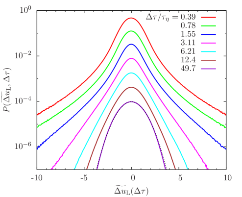
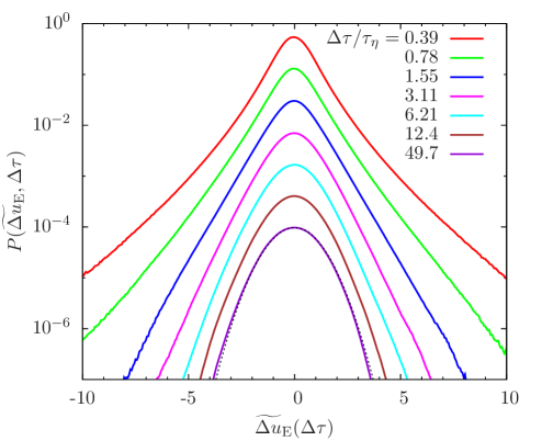
Figure 17.— The normalized PDFs of the Lagrangian (left) and Eulerian (right) temporal velocity differences, $\Delta{u}_{\rm L,E}(\Delta\tau)$, as functions of the time lag. In each curve, the velocity difference is normalized to its rms value, i.e., $\widetilde{\Delta{u}}_{\rm L,E}\equiv\Delta_{\rm L,E}{u}/\langle(\Delta_{\rm L,E}{u})^{2}\rangle^{1/2}$. In both panels, the top lines plot the actual values of the PDFs for $\Delta\tau=0.39\tau_{\eta}$, while each lower line for larger $\Delta\tau$ is shifted downward by a factor of 4 for clarity. The dotted black line corresponds to a Gaussian PDF.

As $\Delta\tau$ decreases, the central part of the PDF keeps a Gaussian-like shape, but the PDF tails become fatter and fatter. The overall PDF shape is highly non-Gaussian at $\Delta\tau\sim\tau_{\eta}$. Fattening of the PDF of $\Delta{u}_{\rm L}$ corresponds to turbulent intermittency in the Lagrangian frame. A comparison of the two panels shows that, at $\Delta\tau\;\hbox to0.0pt{\lower 2.5pt\hbox{$\sim$}\hss}\raise 1.5pt\hbox{$<$}\;6.21\tau_{\eta}$, the PDF tails for $\Delta{u}_{\rm L}$ are significantly fatter than $\Delta{u}_{\rm E}$. This is consistent with the results of previous studies (e.g., Chevillard et al. 2005) that the degree of intermittency in Lagrangian structures is higher than the Eulerian temporal velocity difference.

As the friction time $\tau_{\rm p}$ increases, the flow velocity seen by the particle may make a transition from Lagrangian-like to Eulerian-like. This transition is expected to occur at $\tau_{\rm p}\sim T_{\rm L}\simeq 15\tau_{\eta}$. Interestingly, the PDF shapes of $\Delta{u}_{\rm L}$ and $\Delta{u}_{\rm E}$ are very similar at $\Delta\tau\;\hbox to0.0pt{\lower 2.5pt\hbox{$\sim$}\hss}\raise 1.5pt\hbox{$>$}\;12.4\tau_{\eta}$. This implies that one may use the PDF of $\Delta{u}_{\rm L}$ for all particles to understand the particle-flow relative velocity or the generalized acceleration contribution in the general bidisperse case.

In isotropic turbulence, $\Delta{\boldsymbol{u}}_{\rm E}$ can be related to the spatial velocity difference, $\Delta{\boldsymbol{u}}({\boldsymbol{\ell}})$ ($\equiv{\boldsymbol{u}}({\boldsymbol{x}}+{\boldsymbol{\ell}},t)-{\boldsymbol{u}}({\boldsymbol{x}},t)$), by the so-called random Taylor hypothesis (e.g., Tennekes 1975). In this hypothesis, $\Delta_{\rm E}{u}(\Delta\tau)$ is estimated by $\Delta{u}({\ell})$ at a scale of $\ell\simeq u^{\prime}\Delta\tau$, where it is assumed that the sweeping speed at which the energy-containing eddies advect small-scale eddies across a given point is given by the rms flow velocity, $\sim u^{\prime}$. The hypothesis is supported by a comparison of the PDF shape of $\Delta_{\rm E}{u}(\Delta\tau)$ with the spatial velocity increment $\Delta u_{\rm t}(\ell)$ in the transverse direction at $\ell\simeq\sqrt{3}u^{\prime}\Delta\tau$ in our flow. We also find that the intermittency of temporal structures in the Lagrangian frame is stronger than the Eulerian spatial structures, consistent with previous studies (e.g., Chevillard et al. 2005). The normalized PDF of $\Delta u_{\rm t}(\ell)$ has been examined in details in Appendix B (right panel of Fig. 21) of Paper I.

Appendix B The acceleration and velocity gradient PDFs of the simulated flow

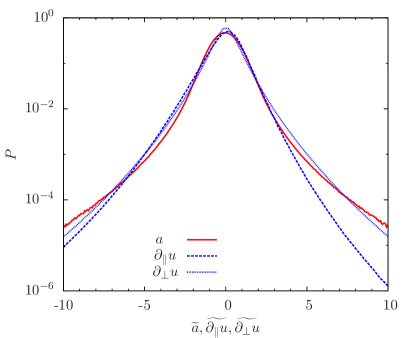
Figure 18.— The normalized PDFs of the acceleration (red), and the longitudinal and transverse velocity gradients, $\partial_{\parallel}u$ and $\partial_{\perp}u$.

In the small particle limit with $\tau_{\rm p}\to 0$, the generalized acceleration and the generalized shear contributions are related to the acceleration, ${\boldsymbol{a}}$, and the spatial gradient, $\partial_{j}u_{i}$, of the flow velocity, respectively (see §2). It is therefore of interest to compare the PDF shape of the acceleration and velocity gradients. Since ${\boldsymbol{a}}=\lim_{\Delta\tau\to 0}\Delta_{\rm L}{\boldsymbol{u}}/\Delta\tau$, the PDF of ${\boldsymbol{a}}$ can be obtained from the Lagrangian velocity difference $\Delta_{\rm L}{\boldsymbol{u}}(\Delta\tau)$ at small $\Delta\tau$. In our simulated flow, the PDF shape of $\Delta_{\rm L}{\boldsymbol{u}}(\Delta\tau)$ is found to be invariant at $\Delta\tau\leq 0.19\tau_{\eta}$, and we can thus measure the PDF of ${\boldsymbol{a}}$ at $\Delta\tau\simeq 0.19\tau_{\eta}$. Similarly, the velocity gradient can be obtained from $\Delta{\boldsymbol{u}}({\boldsymbol{\ell}})$ at small ${\boldsymbol{\ell}}$. We consider the longitudinal ($\Delta u_{\rm r}$) and transverse ($\Delta u_{\rm t}$) components of $\Delta{\boldsymbol{u}}({\boldsymbol{\ell}})$ along and perpendicular to ${\boldsymbol{\ell}}$, and define the longitudinal and transverse velocity gradients as $\partial_{\parallel}u\equiv\lim_{\ell\to 0}\Delta u_{\rm r}(\ell)/\ell$ and $\partial_{\perp}u\equiv\lim_{\ell\to 0}\Delta u_{\rm t}(\ell)/\ell$, respectively. We compute the PDFs of the two gradients from $\Delta u_{\rm r}(\ell)$ and $\Delta u_{\rm t}(\ell)$ across a distance of $\ell\simeq 1.7\eta$, below which the PDF shape converges. In Fig. 18, we show the measured PDFs of $a$ (red), $\partial_{\parallel}u$ and $\partial_{\perp}u$ (blue), respectively. All the PDFs are normalized to have unit variance. The acceleration PDF shown here is for one component of ${\boldsymbol{a}}$. Clearly, the acceleration PDF is slightly fatter than the transverse velocity gradient. The longitudinal velocity gradient is skewed toward negative values, and, as discussed in Paper I, this asymmetry is related to the dissipative nature of turbulence.

Appendix C The tangential PDFs of approaching and separating pairs at fixed Stoke ratios

In Fig. 19, we compare the PDFs, $P(w_{\rm t}|w_{\rm r}\lessgtr 0;f,St_{h})$, of the tangential relative velocity for approaching (solid) and separating (dashed) particle pairs at a distance of $1\eta$. The left and right panels plot the results for $f=\frac{1}{2}$ and $\frac{1}{8}$, respectively. The two panels are plot in a similar way as the right panel of Fig. 13 in Paper I for equal-size particles ($f=1$), which showed that, for $St\;\hbox to0.0pt{\lower 2.5pt\hbox{$\sim$}\hss}\raise 1.5pt\hbox{$<$}\;6.21$, the PDF tails for approaching particles ($w_{\rm r}<0$) are broader than the separating ones ($w_{\rm r}<0$). As discussed in Paper I, one reason for this asymmetry is that the particle distance for approaching pairs backward in time tends to be larger than that for separating ones, especially in the near past.

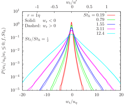
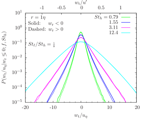
Figure 19.— The PDF of the tangential relative velocity, $w_{\rm t}$, for approaching (solid) and separating (dashed) particle pairs at a distance of $r=1\eta$. In the left and right panels, the Stokes number ratio is fixed at $f=\frac{1}{2}$ and $\frac{1}{8}$, respectively.

As seen in Fig. 19, the asymmetry is present also in the bidisperse case. The difference between the tangential PDFs conditioned on $w_{\rm r}<0$ and $w_{\rm r}>0$ comes only from the shear contribution, as the acceleration contribution does not depend on the relative motions of the two particles (see §2). A comparison of the right panel of Fig. 13 in Paper I for the monodisperse case and the two panels in Fig.  19 here shows that, at the same $St_{h}$, the difference in the tangential PDFs for $w_{\rm r}<0$ and $w_{\rm r}>0$ is smaller for smaller values of $f$. This is because the generalized acceleration term makes a larger contribution when the Stokes number difference increases. The presence of the acceleration contribution makes it easier for the tangential PDFs of approaching and separating pairs to equalize in the bidisperse case.

References

- (1)
- (2) Bec, J., Biferale, L. , Boffetta, G., Celani, A., Cencini, M., et al. 2006, J. Fluid Mech, 550, 349
- (3) Bec, J., Biferale, L., Cencini, M., Lanotte, A. S. & Toschi, F. 2010, J. Fluid Mech. 645, 497
- (4) Bec, J., Biferale, L., Cencini, M., Lanotte, A. S., & Toschi F. 2011, J. Phys.: Conf. Ser. 333, 012003
- (5) Bewley, G. P., Saw, E.-W. & Bodenschatz, E. 2013. New J. Physics, 15, 083051
- (6) Birnstiel, T., Ormel, C. W., & Dullemond, C. P. 2011, A&A, 525, 11
- (7) Blum, J. & Wurm, G. 2008, ARAA, 46, 21
- (8) Brandenburg, A. & Dobler, W. 2002, Computer Physics Communications, 147, 471
- (9) Cate, A.T., Dersken, J., Portela, L. , & Akker, H.V.D. 2004, J. Fluid Mech. 519, 233.
- (10) Chevillard, L., Roux, S. G., Leveque, E., Mordant, N., Pinton, J.-F., & Arneodo, A. 2005, Phys. Rev. Lett., 95, 064501
- (11) Cuzzi, J. N. & Hogan R. C. 2003, Icarus,164, 127
- (12) Cuzzi, J. N., Hogan, R. C., Paque, J. M., & Dobrovolskis, A. R. 2001, ApJ, 546, 496
- (13) de Jong J., Salazar, J. P. L. C., Woodward, S. H., Collins, L. R., & Meng, H. 2010, Int. J. Multiphase Flow, 36, 324
- (14) Dullemond, C. P. & Dominik, C. 2005, A&A, 434, 971
- (15) Falkovich, G., Fouxon, A., & Stepanov, M. G. 2002, Nature, 419, 151
- (16) Falkovich, G. & Pumir, A. 2007, J. Atmos. Sci. 64, 4497
- (17) Frisch, U. 1995, Turbulence. The Legacy of AN Kolmogorov (Cambridge University Press, Cambridge)
- (18) Garaud, P., Meru, F., Galvagni, M., & Olczak, C. 2013, ApJ, 764, 146
- (19) Gualtieri, P., Picano, F., Sardina, G. & Casciola, C. M. 2012. Physica D, 241, 245
- (20) Gustavsson, K. & Mehlig, B. 2011, Phys. Rev. E, 84, 045304(R)
- (21) Gustavsson, K., Mehlig, B., Wilkinson, M. & Uski, V. 2008, Phys. Rev. Lett., 101, 174503
- (22) Gustavsson, K., Meneguz, E., Reeks, M. & Mehlig, B. 2012, New J. Physics, 14, 115017
- (23) Gustavsson, K. & Mehlig, B. 2014, Journal of Turbulence 15, 34
- (24) Güttler, C., Blum, J., Zsom, A., Ormel, C. W.,& Dullemond, C. P. 2010, A&A, 513, A56
- (25) Hubbard, A. 2012, MNRAS, 426, 784
- (26) Hubbard, A. 2013, MNRAS, 432, 1274
- (27) Ishihara, T., Kaneda, Y., Yokokawa, M. Itakura, K. and Uno, A. 2007, J. of Fluid Mech., 592, 335
- (28) Johansen, A., Oishi, J. S., Low, M.-M. M., et al. 2007, Nature, 448, 1022 (Supplemental Material)
- (29) Johansen, A. & Youdin, A. N. 2007, ApJ, 662, 627
- (30) Johansen, A., Youdin, A., & Klahr, H. 2009, ApJ, 697, 1269
- (31) Lanotte, A. S., Bec, J., Biferale, L., Cencini, M., & Toschi, F. 2011. J. Phys.: Conference Series 318, 052010.
- (32) Markiewicz, W. J., Mizuno, H. & Voelk, H. J. 1991, A&A, 242, 286
- (33) Monin, A. S. & Yaglom, A. M. 1975, Statistical Fluid Mechanics: Mechanics of Turbulence, vol. 2. MIT press.
- (34) Mordant, N., Metz, P. , Michel, O., & Pinton, J.-F. 2001, Phys. Rev. Lett. 87, 214501
- (35) Ormel, C. W., & Cuzzi, J. N. 2007, A&A, 466, 413
- (36) Pan, L. & Padoan, P. 2010, J. of Fluid Mech., 661, 73 (PP10)
- (37) Pan, L. & Padoan, P. 2013, ApJ, 776, 12 (Paper I)
- (38) Pan, L. & Padoan, P., & Scalo, J. 2014, submitted, astro-ph: 1403.3865 (Paper II)
- (39) Pan, L., Padoan, P.. Scalo, J., Kritsuk, A. G., & Norman, M. L. 2011, ApJ, 740, 21
- (40) Paret, J. & Tabeling, P 1998, Phys. Fluids, 10, 3126
- (41) Saffman, P. G. & Turner, J. S.1956 J. Fluid Mech., 1, 16
- (42) Salazar J. P. L. C. & Collins L. R. 2012, J. of Fluid Mech., 696, 45
- (43) Sundaram, S., & Collins, L. R. 1997, J. of Fluid Mech., 335, 75
- (44) Tennekes, H. 1975, JFM, 67, 561
- (45) Testi, L., Birnstiel, T., Ricci, L. et al. 2014, astro-ph:1402.1354
- (46) Volk, H. J., Jones, F. C., Morfill, G. E.& Roeser, S. 1980, A&A, 85, 316–325
- (47) Wang, L.-P., Wexler, A. S., & Zhou, Y. 2000, J. of Fluid Mech., 415, 117
- (48) Weidenschilling, S. J. 1980, Icarus, 44, 172
- (49) Wilkinson, M. & Mehlig, B. 2005, Europhys. Lett., 71, 186
- (50) Wilkinson, M. Mehlig, B., & Bezuglyy, V. 2006, Phys. Rev. Lett., 97, 048501
- (51) Windmark, F., Birnstiel, T., Güttler, C., Blum, J., Dullemond, C. P., & Henning Th. 2012a, A&A, 540, A73
- (52) Windmark, F., Birnstiel, T., Ormel, C. W., & Dullemond, C. P. 2012b, A&A, 544, L16
- (53) Zaichik, L. I. & Alipchenkov, V. M. 2009, New J. Phys., 11, 103018
- (54) Zaichik L. I., Alipchenkov, V. M., Sinaiski, E. G. 2008, Particles in Turbulent Flows. Weinheim: Wiley-VCH
- (55) Zaichik, L. I., Simonin, O. & Alipchenkov, V. M. 2006, Phys. Fluids,18, 035110
- (56) Zhou, Y., Wexler, A. S., & Wang, L.-P. 2001, J. Fluid Mech., 433, 77
- (57) Zsom, A., Ormel, C. W., Dullemond, C. P., & Henning, T. 2011, A&A, 534, A73
- (58) Zsom, A., Ormel, C. W., Güttler, C., Blum, J., & Dullemond, C. P. 2010, A&A, 513, A57
- (59)