Highly frustrated spin-lattice models of magnetism and their quantum phase transitions: A microscopic treatment via the coupled cluster method

Abstract

We outline how the coupled cluster method of microscopic quantum many-body theory can be utilized in practice to give highly accurate results for the ground-state properties of a wide variety of highly frustrated and strongly correlated spin-lattice models of interest in quantum magnetism, including their quantum phase transitions. The method itself is described, and it is shown how it may be implemented in practice to high orders in a systematically improvable hierarchy of (so-called LSUB$m$) approximations, by the use of computer-algebraic techniques. The method works from the outset in the thermodynamic limit of an infinite lattice at all levels of approximation, and it is shown both how the “raw” LSUB$m$ results are themselves generally excellent in the sense that they converge rapidly, and how they may accurately be extrapolated to the exact limit, $m\rightarrow\infty$, of the truncation index $m$, which denotes the only approximation made. All of this is illustrated via a specific application to a two-dimensional, frustrated, spin-half $J^{XXZ}_{1}$–$J^{XXZ}_{2}$ model on a honeycomb lattice with nearest-neighbor and next-nearest-neighbor interactions with exchange couplings $J_{1}>0$ and $J_{2}\equiv\kappa J_{1}>0$, respectively, where both interactions are of the same anisotropic $XXZ$ type. We show how the method can be used to determine the entire zero-temperature ground-state phase diagram of the model in the range $0\leq\kappa\leq 1$ of the frustration parameter and $0\leq\Delta\leq 1$ of the spin-space anisotropy parameter. In particular, we identify a candidate quantum spin-liquid region in the phase space.

1 INTRODUCTION

The coupled cluster method (CCM) Bishop (1998) is one of the most pervasive, most powerful, and most successful of all ab initio formalisms of quantum many-body theory. It has probably been applied to more systems in quantum field theory, quantum chemistry, nuclear, subnuclear, condensed matter, and other areas of physics than any other competing method. The CCM has yielded numerical results which are among the most accurate available for an incredibly wide range of both finite and extended physical systems defined on a spatial continuum. These range from atoms and molecules of interest in quantum chemistry, where the method has long been the recognized “gold standard”, to atomic nuclei; from the electron gas to dense nuclear and baryonic matter; and from models in quantum optics, quantum electronics, and solid-state optoelectronics to field theories of strongly interacting nucleons and pions.

This widespread success for both finite Bartlett (1989) and extended Bishop (1991) physical systems has led to recent applications to corresponding quantum-mechanical systems defined on an extended regular spatial lattice. Such lattice systems are nowadays the subject of intense theoretical study. They include many examples of systems characterized by novel ground states which display quantum order in some region of the Hamiltonian parameter space, delimited by critical values or quantum critical points (QCPs), which mark the corresponding quantum phase transitions. The quantum critical phenomena often differ profoundly from their classical counterparts, and the subtle correlations present usually cannot easily be treated by standard many-body techniques such as perturbation theory or mean-field approximations.

A key challenge for modern quantum many-body theory has been to develop microscopic techniques capable of handling both these novel and more traditional systems. Our recent work, in the field of quantum magnetism, for example, shows that the CCM is clearly able to bridge this divide. We have shown how the systematic inclusion of multispin correlations for a wide variety of quantum spin-lattice problems can be efficiently implemented with the CCM Farnell and Bishop (2004). The method is not restricted to bipartite lattices or to non-frustrated systems, and can thus deal with problems where many alternative techniques, such as the exact diagonalization (ED) of small lattices or quantum Monte Carlo (QMC) simulations, are faced with specific difficulties.

In this paper we illustrate the current power of the CCM to describe accurately the properties of strongly interacting and highly frustrated spin-lattice models of interest in quantum magnetism, especially in two spatial dimensions. The method itself is first briefly reviewed in Sec. 2, where we demonstrate how it may readily be implemented to high orders in a specific, systematically improvable, hierarchy (viz., a localized lattice-animal-based subsystem, LSUB$m$, scheme) of approximations, by the use of computer-algebraic techniques. In order to demonstrate how values for ground-state (GS) properties are obtained, using the CCM, which are fully competitive with those from other state-of-the-art methods, including the much more computationally intensive QMC techniques in the relatively rare (unfrustrated) cases where the latter can readily be applied, we apply it to a specific model of current interest. The model itself, which is a frustrated spin-half ($s=\frac{1}{2}$) antiferromagnet with nearest-neighbor (NN) $J_{1}>0$ and competing next-nearest-neighbor (NNN) $J_{2}>0$ exchange couplings on the honeycomb lattice, both of the anisotropic $XXZ$ type, is described in Sec. 3. Results for the model are presented in Sec. 4, where we demonstrate the ability of the CCM to give an accurate description of the zero-temperature ($T=0$) GS phase diagram of this model, which contains two independent control parameter, viz., the frustration parameter $\kappa\equiv J_{2}/J_{1}$, and the spin anisotropy parameter $\Delta$. The raw LSUB$m$ results themselves are shown to be generally excellent, and we demonstrate explicitly both how they converge rapidly and can also be accurately extrapolated in the truncation index to the exact limit, $m\rightarrow\infty$. We show in Sec. 5 how the results so obtained may be used to construct an accurate $T=0$ GS phase diagram for this model. Finally, in Sec. 6 we present our conclusions.

2 A HONEYCOMB LATTICE MODEL

Low-dimensional spin-lattice models of magnets exhibiting frustration, due either to the underlying lattice geometry or to competing interactions, have been the subject of intense study in recent years, both at the theoretical level and via their experimental realizations either in real materials or in ultracold atoms trapped in optical lattices. Their $T=0$ GS phase diagrams often differ profoundly from their classical ($s\rightarrow\infty$) counterparts, exhibiting, for example, such states without magnetic order as various valence-bond crystalline (VBC) phases or quantum spin-liquid (QSL) states.

Since quantum fluctuations of the order parameter destroy long-range order and hence prevent most types of continuous symmetry breaking in one-dimensional (1D) systems, even at $T=0$, 2D systems occupy a special role for studying QPTs. Since quantum fluctuations are generally weaker for higher values of the spin quantum number $s$, systems with $s=\frac{1}{2}$ typically exhibit the biggest differences from classical behavior. Furthermore, of all regular 2D lattices, one with the lowest coordination number, $z=3$, is the honeycomb lattice. Thus, good prima facie candidate systems for exhibiting novel behavior are spin-half models on the honeycomb lattice, and as a specific model that exhibits both frustration and anisotropy (in spin space), we consider here the so-called $J^{XXZ}_{1}$–$J^{XXZ}_{2}$ model Li et al. (2014). It is shown schematically in Fig. 1(a) and its Hamiltonian is given by

     

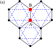
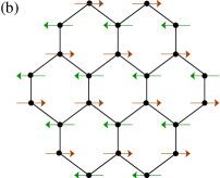
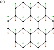
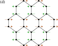
Figure 1: (Color online) The $J^{XXZ}_{1}$–$J^{XXZ}_{2}$ model on the honeycomb lattice, showing (a) the bonds ($J_{1}\equiv$ —– ; $J_{2}\equiv{\color[rgb]{0,0,1}---}$) and the two sites ($\bullet$) A and B of the unit cell; (b) the Néel planar, N(p), state; (c) the Néel $z$-aligned, N($z$), state; and (d) the Néel-II planar, N-II(p), state. The arrows represent the directions of the spins located on lattice sites $\bullet$.

$$H=J_{1}\sum_{\langle i,j\rangle}(s^{x}_{i}s^{x}_{j}+s^{y}_{i}s^{y}_{j}+\Delta s^{z}_{i}s^{z}_{j})+J_{2}\sum_{\langle\langle i,k\rangle\rangle}(s^{x}_{i}s^{x}_{k}+s^{y}_{i}s^{y}_{k}+\Delta s^{z}_{i}s^{z}_{k})\,,$$ (1)

where $\langle i,j\rangle$ and $\langle\langle i,k\rangle\rangle$ denote NN and NNN pairs of spins respectively, and the respective sums count each bond once and once only; and ${\bf s}_{i}=(s^{x}_{i},s^{y}_{i},s^{z}_{i}$) is the $s=\frac{1}{2}$ spin operator on the $i$th site of the honeycomb lattice. We shall be interested in the thermodynamic limit of an infinite lattice ($N\rightarrow\infty$, where $N$ is the number of lattice sites).

The model of Eq. (1) interpolates continuously between the two cases where both NN and NNN exchange couplings have either an isotropic Heisenberg ($XXX$) form when $\Delta=1$ or an isotropic $XY$ ($XX$) form when $\Delta=0$. We shall be interested in the case where both bonds are antiferromagnetic in nature (i.e., when $J_{1}>0$ and $J_{2}>0$), so that they act to frustrate one another. With no further loss of generality we henceforth put $J_{1}\equiv 1$ to set the overall energy scale, and we study the model in the range $0\leq\kappa\leq 1$ of the frustration parameter $\kappa\equiv J_{2}/J_{1}$, and $0\leq\Delta\leq 1$ of the spin anisotropy parameter. Although both limiting isotropic $s=\frac{1}{2}$ models on the honeycomb lattice have been well studied in the past (see, Refs. Varney et al. (2011, 2012); Zhu et al. (2013a); Carrasquilla et al. (2013); Ciolo et al. (2014); Oitmaa and Singh (2014); Bishop et al. (2014) for the $\Delta=0$ $XX$ model and Refs. Rastelli et al. (1979); Fouet et al. (2001); Mulder et al. (2010); Ganesh et al. (2011); Clark et al. (2011); Albuquerque et al. (2011); Mosadeq et al. (2011); Oitmaa and Singh (2011); Mezzacapo and Boninsegni (2012); Li et al. (2012); Bishop et al. (2012, 2013); Ganesh et al. (2013); Zhu et al. (2013b); Gong et al. (2013); Yu et al. (2014) for the $\Delta=1$ $XXX$ model, there is still no overall consensus for either model for its respective complete $T=0$ GS phase diagram in the range of values of $\kappa$ and $\Delta$ under study. What is agreed, however, is that although the two limiting models share exactly the same $T=0$ GS phase diagram in the classical ($s\rightarrow\infty$) case Rastelli et al. (1979); Fouet et al. (2001), their $s=\frac{1}{2}$ counterparts differ significantly. For this reason alone, a complete study of the $T=0$ GS phase diagram of the $s=\frac{1}{2}$ model of Eq. (1) on the honeycomb lattice is of clear interest.

There is broad agreement from various theoretical studies that whereas both classical ($s\rightarrow\infty$) $XX$ and $XXX$ models have Néel ordering for $\kappa<\kappa_{{\rm cl}}=\frac{1}{6}$, their $s=\frac{1}{2}$ counterparts both retain Néel order out to larger values $\kappa_{c_{1}}\approx 0.2$. This finding is completely consistent with the general observation that quantum fluctuations tend to favor collinear forms of magnetic order over noncollinear ones since, in the classical cases, for $\kappa>\kappa_{{\rm cl}}$ the GS phase comprises an infinitely degenerate family of states with spiral magnetic order (and see Refs. Rastelli et al. (1979); Fouet et al. (2001)). These spirally-ordered noncollinear states are very fragile against quantum fluctuations, and there is by now a broad consensus in the literature that neither the $s=\frac{1}{2}$ $XX$ or $XXX$ model has a stable $T=0$ GS phase with noncollinear spiral ordering for any value of $\kappa$ in the range $0\leq\kappa\leq 1$ under study. On the other hand, as $\kappa\rightarrow\infty$, both models reduce to Heisenberg antiferromagnets (HAFs) on two independent triangular lattices, for each of which one knows that the stable GS phase is one where the spins are arranged on three sublattices with relative 120^∘ ordering. Whether such a state is stable against the imposition of NN $J_{1}$ exchange coupling for large but finite values of $\kappa$, or whether it then transforms continuously to a spiral state with a given pitch angle for a specific finite value of $\kappa$, is still unknown. What is broadly agreed, on the other hand, is that any such state only exists for values $\kappa>1$.

The most interesting region for both the $s=\frac{1}{2}$ $XX$ and $XXX$ models is when $\kappa\gtrsim 0.2$. Thus, we know that novel quantum phases often emerge from classical models which have an infinitely degenerate family of GS phases in some region of phase space, as is the case here for the classical $XX$ and $XXX$ models for $\kappa>\kappa_{{\rm cl}}=\frac{1}{6}$. What is typically then found is that quantum fluctuations lift this (accidental) GS degeneracy, either wholly or partially, by the well-known order by disorder mechanism Villain (1977); Villain et al. (1980). Either one or several members, respectively, of the classical family are then favored as the quantum GS phase. For the present $XXX$ model on the honeycomb lattice, for example, it has been shown Mulder et al. (2010) that to leading order, $O(1/s)$, spin-wave fluctuations lift the degeneracy in favor of specific wave vectors, leading to spiral order by disorder.

On the other hand, we know too that quantum fluctuations generally favor collinear ordering over noncollinear ordering, as mentioned above. Hence, one may easily intuit that the strong quantum fluctuations present in the $s=\frac{1}{2}$ models might melt the spiral order for a wide range of values of $\kappa$ in favor of some collinear state. One such clear collinear candidate state is actually among the infinitely degenerate family of ground states at the classical critical point $\kappa=\frac{1}{2}$, at which the closed contours of values of the spiral wave vector, all of which minimize the classical GS energy for a given value of $\kappa$, change character Mulder et al. (2010). This special collinear state among the infinite family of $\kappa=\frac{1}{2}$ ground states is the so-called Néel-II state. It is characterized by having all NN bonds along any one of the three equivalent honeycomb lattice directions as being ferromagnetic (i.e., with spins parallel), while those along the remaining two directions are antiferromagnetic (i.e., with spins antiparallel), as illustrated in Fig. 1(d), for example.

In the extreme $s=\frac{1}{2}$ quantum limit one may also expect quantum fluctuations to destroy completely the magnetic order in any (collinear or noncollinear) quasiclassical state in some region or other of the $T=0$ GS phase space. Just such paramagnetic states have been found by using various theoretical techniques, for both the $s=\frac{1}{2}$ $XX$ and $XXX$ models on the honeycomb lattice, in the interesting regime $0.2\lesssim\kappa\lesssim 0.4$ where, however, the least consensus exists for either model. For the $s=\frac{1}{2}$ $XX$ model, for example, the Néel $xy$ planar [N(p)] ordering that exists for $\kappa<\kappa_{c_{1}}\approx 0.2$ is predicted by different techniques to give way either to a GS phase with Néel $z$-aligned [N($z$)] order Zhu et al. (2013a); Bishop et al. (2014) or to one with a QSL nature Varney et al. (2011); Carrasquilla et al. (2013) in a range $\kappa_{c_{1}}<\kappa<\kappa_{c_{2}}\approx 0.4$. By contrast, for the $s=\frac{1}{2}$ $XXX$ model, the Néel order that exists for $\kappa<\kappa_{c_{1}}$ is variously predicted to give way either to a GS phase with plaquette valence-bond crystalline (PVBC) order Albuquerque et al. (2011); Mosadeq et al. (2011); Li et al. (2012); Bishop et al. (2012, 2013); Ganesh et al. (2013); Zhu et al. (2013b) or to a QSL state Clark et al. (2011); Mezzacapo and Boninsegni (2012); Gong et al. (2013); Yu et al. (2014) in the corresponding range $\kappa_{c_{1}}<\kappa<\kappa_{c_{2}}$.

In the range ($1>$) $\kappa>\kappa_{c_{2}}$ there is broad agreement that for both models there is a strong competition to form the GS phase between states with collinear Néel-II $xy$ planar [N-II(p)] order and staggered-dimer valence-bond crystalline (SDVBC) order, which lie very close in energy to one another. Both of these states break the lattice rotational symmetry in the same way, and are correspondingly threefold-degenerate. Some theoretical treatments also favor a further QCP at $\kappa_{c_{3}}>\kappa_{c_{2}}$, at which a transition occurs between a GS phase with SDVBC ordering for $\kappa_{c_{2}}<\kappa<\kappa_{c_{3}}$, possibility mixed in some or all of this regime with N-II(p) ordering, to one with N-II(p) ordering alone for $\kappa>\kappa_{c_{3}}$. It is interesting to note in this context that alternative techniques such as the ED and density-matrix renormalization group (DMRG) methods, both of which are restricted to lattices with a finite number $N$ of lattice sites, find it particularly difficult to distinguish between the N-II(p) and SDVBC phases in the regime $\kappa>\kappa_{c_{2}}$ in the thermodynamic limit $N\rightarrow\infty$ in which we are interested, for which finite-size scaling is required, especially for the $XX$ model. It is thus particularly valuable to use a size-extensive method such as the CCM used here, which works from the outset in the $N\rightarrow\infty$ limit at every level of LSUB$m$ approximation. Since such LSUB$m$ approximations form well-defined hierarchies, as explained in Sec. 3, the only final extrapolation needed by us is to the exact ($m\rightarrow\infty$) limit in the truncation index $m$. Furthermore, at the highest level of approximation feasible with available computational resources, results for physical quantities are often already very well converged, as our specific results in Sec. 4 for the $s=\frac{1}{2}$ $J^{XXZ}_{1}$–$J^{XXZ}_{2}$ model of Eq. (1) on the honeycomb lattice will show.

3 THE COUPLED CLUSTER METHOD

Since the CCM is well documented in the literature (see, e.g., Refs. Bishop et al. (2012, 2013, 2014); Bishop and Kümmel (1987); Arponen and Bishop (1991); Bishop (1991, 1998); Bishop et al. (1991); Zeng et al. (1998); Farnell et al. (2002); Farnell and Bishop (2004); Bishop et al. (2008)) we present only a brief overview of its key features here. Any CCM calculation starts with the choice of a suitable model state (or reference state), $|\Phi\rangle$, on top of which the quantum correlations present in the exact GS phase under study can be systematically incorporated later, as we describe below. For the present model we use each of the N(p), N($z$), and N-II(p) states shown schematically in Figs. 1(b)–1(d).

Once a model state $|\Phi\rangle$ is chosen, the exact GS ket- and bra-state wave functions that satisfy the corresponding Schrödinger equations,

$$H|\Psi\rangle=E|\Psi\rangle\,;\quad\langle\tilde{\Psi}|H=E\langle\tilde{\Psi}|\,,\quad$$ (2)

are parametrized as

$$|\Psi\rangle={\rm e}^{S}|\Phi\rangle\,;\quad\langle\tilde{\Psi}|=\langle\Phi|\tilde{S}{\rm e}^{-S}\,,$$ (3)

where we use the intermediate normalization scheme for $|\Psi\rangle$, such that $\langle\Phi|\Psi\rangle=\langle\Phi|\Phi\rangle\equiv 1$, and then for $\langle\tilde{\Psi}|$ choose its normalization such that $\langle\tilde{\Psi}|\Psi\rangle=1$. The correlation operators $S$ and $\tilde{S}$ are decomposed in terms of exact sets of multiparticle, multiconfigurational creation and destruction operators, $C^{+}_{I}$ and $C^{-}_{I}\equiv(C^{+}_{I})^{\dagger}$, respectively, as

$$S=\sum_{I\neq 0}{\cal S}_{I}C^{+}_{I}\,;\quad\tilde{S}=1+\sum_{I\neq 0}\tilde{{\cal S}}_{I}C^{-}_{I}\,,$$ (4)

where $C^{+}_{0}\equiv 1$, the identity operator, and $I$ is a set index describing a complete set of single-particle configurations for all of the particles. The reference state $|\Phi\rangle$ thus acts as a fiducial (or cyclic) vector, or generalized vacuum state, with respect to the complete set of creation operators $\{C^{+}_{I}\}$, which are hence required to satisfy the conditions $\langle\Phi|C^{+}_{I}=0=C^{-}_{I}|\Phi\rangle,\forall I\neq 0$.

In order to consider each site on the spin lattice to be equivalent to all others, whatever the choice of state $|\Phi\rangle$, it is convenient to form a passive rotation of each spin so that in its own local spin-coordinate frame it points in the downward, (i.e., negative $z$) direction. Clearly, such choices of local spin-coordinate frames leave the basic SU(2) spin commutation relations unchanged, but have the beneficial effect that the $C^{+}_{I}$ operators can be expressed as products of single-spin raising operators $s^{+}_{k}\equiv s^{x}_{k}+is^{y}_{k}$, such that $C^{+}_{I}\equiv s^{+}_{k_{1}}s^{+}_{k_{2}}\cdots s^{+}_{k_{n}};\;n=1,2,\cdots,2sN$.

The complete set of multiparticle correlation coefficients $\{{\cal S}_{I},{\tilde{\cal S}}_{I}\}$ may now be evaluated by extremizing the energy expectation value $\bar{H}\equiv\langle\tilde{\Psi}|H|\Psi\rangle=\langle\Phi|{\tilde{S}}{\rm e}^{-S}H{\rm e}^{S}|\Phi\rangle$, with respect to each of them, $\forall I\neq 0$. Variation with respect to each coefficient ${\tilde{\cal S}}_{I}$ yields the coupled set of nonlinear equations,

$$\langle\Phi|C^{-}_{I}{\rm e}^{-S}H{\rm e}^{S}|\Phi\rangle=0\,,\quad\forall I\neq 0\,,$$ (5)

for the coefficients $\{{\cal S}_{I}\}$, while variation with respect to each coefficient ${\cal S}_{I}$ yields the corresponding set of linear equations,

$$\langle\Phi|\tilde{S}({\rm e}^{-S}H{\rm e}^{S}-E)C^{+}_{I}|\Phi\rangle=0\,,\quad\forall I\neq 0\,,$$ (6)

for the coefficients $\{{\tilde{\cal S}}_{I}\}$, once the coefficients $\{{\cal S}_{I}\}$ have been calculated from Eq. (5), and where in Eq. (6) we have used Eqs. (2) and (3) to introduce the GS energy $E$.

Up till now everything has been exact. In practice, of course, approximations need to be introduced, and these are made within the CCM by restricting the set of indices $\{I\}$ retained in the expansions of Eq. (4) for the otherwise exact correlation operators $S$ and $\tilde{S}$. One such specific hierarchical scheme, viz., the LSUB$m$ scheme, is described below. It is important to realize, however, that no further approximations are made. In particular, the method is guaranteed by the use of the exponential parametrizations in Eq. (3) to be size-extensive at every level of truncation, and hence we work from the outset in the $N\rightarrow\infty$ limit. Similarly, the important Hellmann-Feynman theorem is also exactly obeyed at every level of truncation. Lastly, when the similarity-transformed Hamiltonian ${\rm e}^{-S}H{\rm e}^{S}$ in Eqs. (5) and (6) is expanded in powers of $S$ using the well-known nested commutator expansion, the fact that $S$ contains only spin-raising operators not only guarantees that all terms are linked, but also that the otherwise infinite expansion actually terminates at a finite order, so that no further approximations are needed.

Once an approximation has been chosen and the retained coefficients $\{{\cal S}_{I},{\tilde{\cal S}}_{I}\}$ have been calculated from Eqs. (5) and (6), any GS quantity can, in principle, be calculated. For example, the GS energy $E$ can be calculated in terms of the coefficients $\{{\cal S}_{I}\}$ alone, as $E=\langle\Phi|{\rm e}^{-S}H{\rm e}^{S}|\Phi\rangle$, while the average on-site GS magnetization (or magnetic order parameter) $M$ needs both sets $\{{\cal S}_{I}\}$ and $\{{\tilde{\cal S}}_{I}\}$ for its evaluation as $M=-\frac{1}{N}\langle\Phi|\tilde{S}{\rm e}^{-S}\sum^{N}_{k=1}s^{z}_{k}{\rm e}^{S}|\Phi\rangle$, in terms of the rotated local spin-coordinate frames defined above.

Thus, the only approximation made in the CCM is to truncate the set of indices $\{I\}$ in the expansions of the correlation operators $S$ and $\tilde{S}$. We use here the well-studied LSUB$m$ scheme Bishop et al. (2012, 2013, 2014, 1991); Zeng et al. (1998); Farnell et al. (2002); Farnell and Bishop (2004); Bishop et al. (2008) in which, at the $m$th level of approximation, one retains all multispin-flip configurations $\{I\}$ defined over no more than $m$ contiguous lattice sites. Such cluster configurations are defined to be contiguous if every site is NN to at least one other. The number, $N_{f}$, of such fundamental configurations is reduced by exploiting the space- and point-group symmetries and any conservation laws that pertain to the Hamiltonian and the model state being used. Even so, $N_{f}$ increases rapidly with increasing LSUB$m$ truncation index $m$, and it becomes necessary to use massive parallelization together with supercomputing resources Zeng et al. (1998), to derive and solve the corresponding coupled sets of CCM equations (5) and (6). For example, we have finally $N_{f}=818\,300$ for the N-II(p) reference state at the LSUB12 level.

Finally, as a last step, we need to extrapolate the approximate LSUB$m$ results to the limit $m\rightarrow\infty$ where the CCM becomes exact. For the GS energy per spin, $e\equiv E/N$, we use the well-tested extrapolation scheme Farnell et al. (2002); Bishop et al. (2012, 2013, 2014, 2008); Farnell and Bishop (2004),

$$e(m)=e_{0}+e_{1}m^{-2}+e_{2}m^{-4}\,,$$ (7)

where results with $m=\{6,8,10,12\}$ are employed for the N(p) and N-II(p) states used as model state, and with $m=\{4,6,8,10\}$ for the N($z$) state. For the magnetic order parameter of systems near a QCP an appropriate extrapolation rule is the “leading power-law” scheme Bishop et al. (2013, 2014),

$$M(m)=c_{0}+c_{1}(1/m)^{c_{2}}\,,$$ (8)

which we use here for the LSUB$m$ results based on the N($z$) state with $m=\{4,6,8,10\}$. An alternative well-tested scheme for systems with strong frustration or where the order in question is zero or close to zero Bishop et al. (2012, 2013, 2014) is

$$M(m)=d_{0}+d_{1}m^{-1/2}+d_{2}m^{-3/2}\,,$$ (9)

when the leading exponent $c_{2}$ in Eq. (8) has been empirically found to be close to 0.5, as is the case here for results based on both the N(p) and N-II(p) model states with $m=\{6,8,10,12\}$.

4 RESULTS

We now firstly present our CCM extrapolated (LSUB$\infty$) results for the GS energy per spin, $E/N$, and magnetic order parameter, $M$, using the extrapolation schemes described above in Sec. 3. For both quantities we present three different curves for each value of the anisotropy parameter $\Delta$ shown, corresponding respectively to calculations based on the N(p), N($z$), and N-II(p) states as our chosen CCM model state.

Results for the GS energy obtained in this way are shown in Fig. 2.

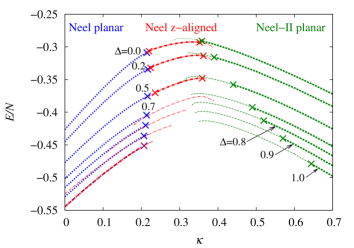
Figure 2: (Color online) The GS energy per spin $E/N$ versus the frustration parameter $\kappa\equiv J_{2}/J_{1}$ for the spin-$\frac{1}{2}$ $J^{XXZ}_{1}$–$J^{XXZ}_{2}$ model on the honeycomb lattice (with $J_{1}=1$), for various values of the anisotropy parameter $\Delta=0.0,0.2,0.5,0.7,0.8,0.9,1.0$ (from top to bottom, respectively). We show extrapolated CCM LSUB$\infty$ results (see text for details) based on the Néel planar, Néel $z$-aligned, and Néel-II planar model states, respectively. The times ($\times$) symbols mark the points where the respective extrapolations for the order parameter have $M\rightarrow 0$, and the unphysical portions of the solutions are shown by thinner lines (see text for details).

A particularly noteworthy feature of the curves shown is that they all exhibit termination points. Thus, the N(p) curves all end at corresponding upper termination points, while the N-II(p) curves end at corresponding lower termination points. The intermediate N($z$) curves end at both corresponding lower and upper termination points. In each case the respective termination points relate to those points beyond which real solutions for the CCM multiconfigurational correlation coefficients $\{{\cal S}_{I}\}$ cease to exist in the LSUB$m$ approximation with the highest value of the truncation index $m$ used, for the particular extrapolated curve shown. Such termination points of LSUB$m$ solutions are both well understood and well documented in the literature (see, e.g., Refs. Farnell and Bishop (2004); Bishop et al. (2014, 2012, 2013)). They are simply approximate manifestations of a corresponding QCP in the system, beyond which the order associated with the model state being employed melts. As would then be expected, we find for a given value of $\Delta$ that as the index $m$ is increased the range of values of $\kappa$ for which the LSUB$m$ equations have real solutions becomes narrower. Eventually, as $m\rightarrow\infty$, each termination point then becomes the respective exact QCP. Clearly, from what has just been explained, real LSUB$m$ solutions with a fixed finite value of $m$ can hence also exist in regions where the corresponding magnetic order is destroyed (i.e., where $M<0$).

Corresponding sets of curves to those shown in Fig. 2 for the GS energy per spin, $E/N$, are shown in Fig. 3 for the magnetic order parameter, $M$.

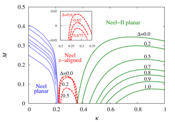
Figure 3: (Color online) The GS magnetic order parameter $M$ versus the frustration parameter $\kappa\equiv J_{2}/J_{1}$ for the spin-$\frac{1}{2}$ $J^{XXZ}_{1}$–$J^{XXZ}_{2}$ model on the honeycomb lattice (with $J_{1}>0$) for various values of the anisotropy parameter $\Delta=0.0,0.2,0.5,0.7,0.8,0.9,1.0$ (from top to bottom, respectively). We show extrapolated CCM LSUB$\infty$ results (see text for details) based on the Néel planar, Néel $z$-aligned, and Néel-II planar states as CCM model states, respectively.

In Fig. 2 we show by times ($\times$) symbols those points on each curve where $M=0$, as determined from the corresponding extrapolated LSUB$\infty$ curve in Fig. 3. In Fig. 2 we also denote by thinner lines those portions of the curves which are “unphysical” in the sense that $M<0$, by contrast with the corresponding “physical” regions where $M>0$, which pertain to those portions of the curves denoted by thicker lines.

We can immediately draw several conclusions from the results shown in Figs. 2 and 3. Firstly, it is clear that N(p) order is present, for all values of $\Delta$ shown, below a lower critical value, $0<\kappa<\kappa_{c_{l}}(\Delta)$. Furthermore, $\kappa_{c_{l}}$ depends only very weakly on $\Delta$, taking the value $\kappa_{c_{l}}(\Delta)\approx 0.21$. Secondly, we observe both that N($z$) order is present within a rather narrow range of values around $\kappa\approx 0.3$ for $\Delta\lesssim 0.66$, but that it becomes unstable for $\Delta\gtrsim 0.66$. Thirdly, it is also clear that N-II(p) order is present, for all values of $\Delta$ shown, above some upper critical value, $\kappa_{c_{u}}(\Delta)<\kappa$ $(<1)$, where $\kappa_{c_{u}}(\Delta)$ increases monotonically with $\Delta$. Fourthly, it is particularly clear from Fig. 3 that the GS phases with N(p) and N($z$) order melt at (or very close to) the same value $\kappa_{c_{l}}(0)$ for $\Delta=0$, but as $\Delta$ is increased a very narrow region (in $\kappa$) opens up between these two phases in which the GS phase has neither of these orderings. Finally, Fig. 3 similarly shows that although the two GS phases with N($z$) and N-II(p) order also melt at (or very close to) the same value $\kappa_{c_{u}}(0)$ for $\Delta=0$, as $\Delta$ is increased a GS phase with neither of these forms of order opens up between them. The range (in $\kappa$) of stability of this intermediate phase increases monotonically with $\Delta$.

We now turn to the issue of what might be the nature of the remaining GS phases outside the regimes of stability of the quasiclassical N(p), N($z$), and N-II(p) phases, as discussed above. Once we have identified any possible candidate phase with a specific form of ordering, described by a suitable operator $\hat{O}$, a very convenient way to test for the relative stability of a GS phase built on a given CCM model state against that new form of ordering is to consider its linear response to an imposed perturbation with a corresponding field operator, $F=\delta\,\hat{O}$, added to the original system Hamiltonian [i.e., of Eq. (1) for the present case], where $\delta$ is a (positive) infinitesimal. The perturbed energy per spin, $e(\delta)\equiv E(\delta)/N$, is then calculated at various LSUB$m$ levels of approximation based on the CCM model state whose stability is being investigated, for the infinitesimally perturbed Hamiltonian $H+F$. The corresponding susceptibility of the system to this perturbation is then defined, as usual, (and see, e.g., Refs. Bishop et al. (2014, 2012, 2013)) as

$$\chi\equiv-\left.\frac{\partial^{2}{e(\delta)}}{\partial{\delta}^{2}}\right|_{\delta=0}.$$ (10)

The GS order of the CCM model state will thus become unstable against formation of the imposed form of order when $\chi\rightarrow\infty$ or, equivalently, when $1/\chi\rightarrow 0$. The corresponding LSUB$m$ results for the susceptibility of the given CCM model state against the imposed form of order are then extrapolated to the LSUB$\infty$ limit using the unbiased “leading power-law” scheme,

$$\chi^{-1}(m)=x_{0}+x_{1}(1/m)^{\nu}\,,$$ (11)

similar to that in Eq. (8) for the order parameter.

Previous results using the CCM for the current model of Eq. (1) in the limiting cases of the $XX$ model Bishop et al. (2014) at $\Delta=0$ and the $XXX$ model Bishop et al. (2012, 2013) at $\Delta=1$, as well as those using alternative techniques, suggest that N-II(p) ordering strongly competes with SDVBC ordering to form the stable GS phase in the relevant part of phase space. Hence, we now perform CCM calculations based on the N-II(p) state as model state where the perturbing field promotes SDVBC order, $\hat{O}\rightarrow\hat{O}_{d}$, as illustrated schematically in the right-hand frame of Fig. 4.

 

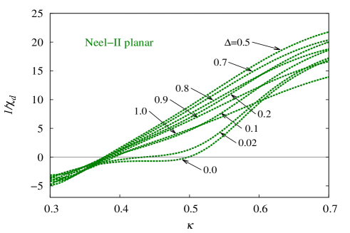
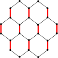
Figure 4: (Color online) Left: The inverse staggered dimer susceptibility, $1/\chi_{d}$, versus the frustration parameter, $\kappa\equiv J_{2}/J_{1}$, for the spin-$\frac{1}{2}$ $J^{XXZ}_{1}$–$J^{XXZ}_{2}$ model on the honeycomb lattice (with $J_{1}=1$) for various values of the anisotropy parameter $\Delta$. We show extrapolated CCM LSUB$\infty$ results (see text for details) based on the Néel-II planar state as CCM model state. Right: The field $F\rightarrow\delta\;\hat{O}_{d}$ for the staggered dimer susceptibility, $\chi_{d}$. Thick (red) and thin (black) lines correspond respectively to strengthened and unaltered NN exchange couplings, where $\hat{O}_{d}=\sum_{\langle i,j\rangle}a_{ij}(s^{x}_{i}{s}^{x}_{j}+s^{y}_{i}{s}^{y}_{j}+\Delta s^{z}_{i}{s}^{z}_{j})$, and the sum runs over all NN bonds, with $a_{ij}=+1$ and 0 for thick (red) lines and thin (black) lines respectively.

The results presented in Fig. 4 for the corresponding inverse staggered dimer susceptibility, $1/\chi_{d}$, are LSUB$\infty$ extrapolations based on Eq. (11), with LSUB$m$ results $m=\{4,6,8\}$ used as input, for each of the values of $\Delta$ shown. They show clearly that the lower critical value of the frustration parameter $\kappa$ at which SDVBC order appears is rather insensitive to the value of the spin anisotropy parameter $\Delta$ for all $\Delta\gtrsim 0.1$, where it takes the almost constant value $\kappa\approx 0.38$. However, the locus of such SDVBC critical points meets the corresponding locus of critical points $\kappa_{c_{u}}(\Delta)$ above which N-II(p) order appears, as taken from Fig. 3, at a value $\Delta\approx 0.1$. Hence, for values $\Delta\lesssim 0.1$, a “mixed” region opens up in the $T=0$ GS phase diagram in which both SDVBC and N-II(p) forms of order appear to coexist over a fairly narrow range of values of $\kappa$, above which N-II(p) order then reasserts itself as the sole form of ordering in the GS phase.

We turn finally to the remaining, and especially interesting, region in the $\kappa$–$\Delta$ phase space, which is outside the region of N(z) stability but between the two curves $\kappa=\kappa_{c_{l}}(\Delta)\approx 0.21$ (below which N(p) order is stable) and $\kappa\approx 0.38$ (above which SDVBC and/or N-II(p) order is stable). For the limiting case of the $XXX$ model (at $\Delta=1$) some methods (including the CCM) favor the GS phase to have PVBC order over all or part of this region Albuquerque et al. (2011); Mosadeq et al. (2011); Li et al. (2012); Bishop et al. (2012, 2013); Ganesh et al. (2013); Zhu et al. (2013b); Gong et al. (2013), while others favor a QSL state Clark et al. (2011); Mezzacapo and Boninsegni (2012); Gong et al. (2013); Yu et al. (2014), again over all or part of the region. Hence, we now perform CCM calculations based on the N(p) state as model state, in the presence of a perturbing field that now promotes PVBC order, $\hat{O}\rightarrow\hat{O}_{p}$, as shown schematically in the right-hand frame of Fig. 5.

 

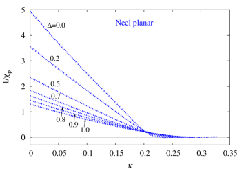
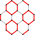
Figure 5: (Color online) Left: The inverse plaquette susceptibility, $1/\chi_{p}$, versus the frustration parameter, $\kappa\equiv J_{2}/J_{1}$, for the spin-$\frac{1}{2}$ $J^{XXZ}_{1}$–$J^{XXZ}_{2}$ model on the honeycomb lattice (with $J_{1}=1$) for various values of the anisotropy parameter $\Delta$. We show extrapolated CCM LSUB$\infty$ results (see text for details) based on the Néel planar state as CCM model state. Right: The field $F=\delta\,\hat{O}_{p}$ for the plaquette susceptibility $\chi_{p}$. Thick (red) and thin (black) lines correspond respectively to strengthened and weakened NN exchange couplings, where $\hat{O}_{p}=\sum_{\langle i,j\rangle}a_{ij}(s^{x}_{i}{s}^{x}_{j}+s^{y}_{i}{s}^{y}_{j}+\Delta s^{z}_{i}{s}^{z}_{j})$, and the sum runs over all NN bonds, with $a_{ij}=+1$ and $-1$ for thick (red) and thin (black) lines respectively.

The results presented in Fig. 5 for the corresponding inverse plaquette susceptibility, $1/\chi_{p}$, are again LSUB$\infty$ extrapolations based on Eq. (11), with LSUB$m$ results $m=\{4,6,8\}$ used as input, for each of the values of $\Delta$ shown. Once again, they show clear evidence for corresponding regions of stability of a GS phase with PVBC order.

5 $T=0$ GS PHASE DIAGRAM

On the basis of the results presented so far in Sec. 4 it is now straightforward to construct the $T=0$ GS phase digram for the model, as shown in Fig. 6.

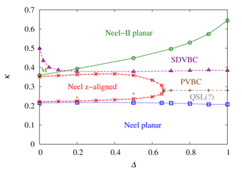
Figure 6: (Color online) Phase diagram for the spin-$\frac{1}{2}$ $J^{XXZ}_{1}$–$J^{XXZ}_{2}$ model on the honeycomb lattice (with $J_{1}>0$ and $\kappa\equiv J_{2}/J_{1}>0$) in the window $0\leq\kappa\leq 1$ and $0\leq\Delta\leq 1$, as obtained by a CCM analysis. The phase in the region marked “M” has both SDVBC and Néel-II planar order. See text for details.

Clearly, the regions of stability of the N(p), N($z$), and N-II(p) phases may be taken from Fig. 3 as those in which the respective magnetic order parameters $M$ take positive values. The corresponding points at which $M=0$ are shown in Fig. 6 by open square ($\square$), times ($\times$), and open circle ($\bigcirc$) symbols, respectively. Similarly, the points at which $\chi^{-1}_{d}\rightarrow 0$ and $\chi^{-1}_{p}\rightarrow 0$, taken from Figs. 4 and 5, are shown in Fig. 6 by open triangle ($\triangle$) and plus ($+$) symbols, respectively. The small region of mixed SDVBC and N-II(p) order, described in Sec. 4, is denoted in Fig. 6 by “M”.

Based on the results for $1/\chi_{p}$ from Fig. 5 we now tentatively identify the region denoted by “PVBC” in Fig. 6 as having stable PVBC order. The remaining region denoted by “QSL(?)” is a clear candidate for a QSL phase, since we find no evidence for any form of magnetic (spin) ordering, nor of either form of VBC ordering, for which we have tested. In this context we also mention that a recent DMRG study Gong et al. (2013) of the limiting $XXX$ case (i.e., $\Delta=1$) of the present model found solid evidence of (weak) PVBC order in the thermodynamic ($N\rightarrow\infty$) limit, in the range $0.26\lesssim\kappa\lesssim 0.35$ of the frustration parameter, in good agreement with our own estimate for this limiting $XXX$ case that PVBC order exists in the range $0.28\lesssim\kappa\lesssim 0.38$. Very interestingly, the same DMRG study Gong et al. (2013) excluded, in the same thermodynamic limit, any form of either magnetic (spin) or VBC ordering in the range $0.22\lesssim\kappa\lesssim 0.26$ immediately above the Néel-ordered regime for the $XXX$ model, which was identified as being the stable GS phase for $\kappa\lesssim 0.22$. These DMRG findings were thus consistent with a QSL phase in the region $0.22\lesssim\kappa\lesssim 0.26$, again in broad agreement with our own tentative conclusion of a QSL phase in the region $0.21\lesssim\kappa\lesssim 0.28$ for the $XXX$ limiting case of the model. Indeed, these results are backed up by our earlier CCM analysis Bishop et al. (2012) of the $s=\frac{1}{2}$ $J_{1}$–$J_{2}$ $XXX$ model on the honeycomb lattice.

Thus, it was noted already in Ref. Bishop et al. (2012) that the transition from the N(p) phase to the PVBC phase in the $XXX$ model might be via an intermediate phase. Any such intermediate phase was estimated to be restricted to a region $\kappa_{c_{1}}<\kappa<\kappa_{c_{1}}^{\prime}$. The value of $\kappa_{c_{1}}$ was accurately obtained from the point where Néel order vanishes as $\kappa_{c_{1}}=0.207(3)$, and it is identical to that now shown in Fig. 6 by the open square ($\square$) symbol at $\Delta=1$. The high accuracy obtained for $\kappa_{c_{1}}$ essentially stems from the shape of the N(p) order curve shown in Fig. 3, with its very steep (or infinite) slope at the point $\kappa_{c_{1}}$ where $M\rightarrow 0$. By contrast, the point $\kappa_{c_{1}}^{\prime}$ was determined as in Fig. 5 from the point where $1/\chi_{p}\rightarrow 0$. The relative inaccuracy in this value stems, conversely from the very shallow (or zero) slope in the $1/\chi_{p}$ curve at the point $\kappa_{c_{1}}^{\prime}$ where it becomes zero. In the earlier CCM analysis Bishop et al. (2012) a value $\kappa_{c_{1}}^{\prime}\approx 0.24$ was quoted, without an error estimation. In the current analysis we have specifically examined the lower phase boundary of the PVBC phase in greater detail, and our best estimate for the limiting $XXX$ model is now $\kappa_{c_{1}}^{\prime}\approx 0.28(2)$ from Fig. 5, and as shown in Fig. 6 by the plus ($+$) symbol at $\Delta=1$. Nevertheless, it is still the case that of all the phase boundaries shown in Fig. 6, the one between the PVBC and putative QSL phases probably has the largest uncertainty, with a similar error along its whole length to that quoted above at the point $\Delta=1$. In this context we note too that Fig. 6 shows that the plus ($+$) symbols denoting the lower boundary of PVBC stability do not fall precisely on top of the times ($\times$) symbols that denote the lower boundary of stability of the N($z$) phase, in the region $\Delta\lesssim 0.66$ where the latter phase exists as a stable GS phase. This difference is probably also another independent indication of the error bars associated with the lower PVBC boundary points.

These error bars could certainly be reduced by including higher-order LSUB$m$ results in the extrapolations. The entire PVBC and SDVBC regions of stability would also more definitively be confirmed by performing calculations of $1/\chi_{p}$ and $1/\chi_{d}$ based on other CCM model states to confirm their respective boundaries. For example, for the PVBC phase one might also use the N-II(p) state as CCM model state to confirm the upper boundary of the phase. In any case, more definitive evidence awaits higher-order LSUB$m$ calculations. Without them, for example, the possibility of a stable QSL phase also existing in the very narrow region between the N($z$) and SDVBC phases for $\Delta\lesssim 0.66$ also cannot be ruled out.

6 CONCLUSIONS

In this paper we have outlined how the well-known CCM technique, which has been very widely and very successfully applied to diverse (both finite and macroscopically extended) physical systems that exist in a spatial continuum, can be adapted for use with spin-lattice models of interest in quantum magnetism, in which the spins are confined to the sites of a regular periodic spatial lattice. In particular, we have explained how it may be applied, with comparable success, to high orders in a systematically improvable hierarchy of approximations. The method acts at every level of truncation in the thermodynamic limit ($N\rightarrow\infty$), and the only approximation made in practice is to a given $m$th level in the approximation hierarchy. Thus, unlike in such alternative techniques as ED and QMC methods, no finite-size scaling is ever needed within the CCM. We have also shown how GS quantities may readily be extrapolated to the exact $m\rightarrow\infty$ limit of the truncation scheme, by the use of well-tested heuristic schemes.

As an illustration of the CCM technique we applied it here to the two-dimensional, frustrated, spin-half $J^{XXZ}_{1}$–$J^{XXZ}_{2}$ model on the honeycomb lattice. We demonstrated explicitly how a CCM analysis of the model could yield a fully coherent and accurate picture of its full $T=0$ GS phase diagram. We identified, in particular, a specific region in the phase space in which we positively excluded magnetic and VBC forms of order, and which is hence a strong candidate for a QSL phase. Clearly, it would be of value to apply other techniques to this model in order to check our findings.

We note finally that the CCM has been applied with comparable success in recent years to many other spin-lattice problems. Particular strengths of the method are that at every level of approximation it obeys both the Goldstone linked-cluster theorem (in the sense that it is manifestly size-extensive) and, perhaps even more importantly, the Hellmann-Feynman theorem.

In conclusion, we hope that we have convinced the reader that the CCM is extremely versatile, requiring only the choice of a suitable model state (or set of such states) as input, on top of which the method incorporates the multispin correlations systematically. Although we have demonstrated its use here for the case of a spin-half system, it is quite straightforward to generalize the CCM for use with spins of arbitrary quantum number $s$ Farnell et al. (2002).

References

- Bishop (1998) R. F. Bishop, “The Coupled Cluster Method,” in Microscopic Quantum Many-Body Theories and Their Applications, edited by J. Navarro, and A. Polls, Lecture Notes in Physics Vol. 510, Springer-Verlag, Berlin, 1998, p. 1.
- Bartlett (1989) R. J. Bartlett, J. Phys. Chem. 93, 1697 (1989).
- Bishop (1991) R. F. Bishop, Theor. Chim. Acta 80, 95 (1991).
- Farnell and Bishop (2004) D. J. J. Farnell, and R. F. Bishop, “The Coupled Cluster Method Applied to Quantum Magnetism,” in Quantum Magnetism, edited by U. Schollwöck, J. Richter, D. J. J. Farnell, and R. F. Bishop, Lecture Notes in Physics Vol. 645, Springer-Verlag, Berlin, 2004, p. 307.
- Li et al. (2014) P. H. Y. Li, R. F. Bishop, and C. E. Campbell, Phys. Rev. B 89, 220408(R) (2014).
- Varney et al. (2011) C. N. Varney, K. Sun, V. Galitski, and M. Rigol, Phys. Rev. Lett. 107, 077201 (2011).
- Varney et al. (2012) C. N. Varney, K. Sun, V. Galitski, and M. Rigol, New J. Phys. 14, 115028 (2012).
- Zhu et al. (2013a) Z. Zhu, D. A. Huse, and S. R. White, Phys. Rev. Lett. 111, 257201 (2013a).
- Carrasquilla et al. (2013) J. Carrasquilla, A. D. Ciolo, F. Becca, V. Galitski, and M. Rigol, Phys. Rev. B 88, 241109(R) (2013).
- Ciolo et al. (2014) A. D. Ciolo, J. Carrasquilla, F. Becca, M. Rigol, and V. Galitski, Phys. Rev. B 89, 094413 (2014).
- Oitmaa and Singh (2014) J. Oitmaa, and R. R. Singh, Phys. Rev. B 89, 104423 (2014).
- Bishop et al. (2014) R. F. Bishop, P. H. Y. Li, and C. E. Campbell, Phys. Rev. B 89, 214413 (2014).
- Rastelli et al. (1979) E. Rastelli, A. Tassi, and L. Reatto, Physica B & C 97, 1 (1979).
- Fouet et al. (2001) J. B. Fouet, P. Sindzingre, and C. Lhuillier, Eur. Phys. J. B 20, 241 (2001).
- Mulder et al. (2010) A. Mulder, R. Ganesh, L. Capriotti, and A. Paramekanti, Phys. Rev. B 81, 214419 (2010).
- Ganesh et al. (2011) R. Ganesh, D. N. Sheng, Y.-J. Kim, and A. Paramekanti, Phys. Rev. B 83, 144414 (2011).
- Clark et al. (2011) B. K. Clark, D. A. Abanin, and S. L. Sondhi, Phys. Rev. Lett. 107, 087204 (2011).
- Albuquerque et al. (2011) A. F. Albuquerque, D. Schwandt, B. Hetényi, S. Capponi, M. Mambrini, and A. M. Läuchli, Phys. Rev. B 84, 024406 (2011).
- Mosadeq et al. (2011) H. Mosadeq, F. Shahbazi, and S. A. Jafari, J. Phys.: Condens. Matter 23, 226006 (2011).
- Oitmaa and Singh (2011) J. Oitmaa, and R. R. P. Singh, Phys. Rev. B 84, 094424 (2011).
- Mezzacapo and Boninsegni (2012) F. Mezzacapo, and M. Boninsegni, Phys. Rev. B 85, 060402(R) (2012).
- Li et al. (2012) P. H. Y. Li, R. F. Bishop, D. J. J. Farnell, and C. E. Campbell, Phys. Rev. B 86, 144404 (2012).
- Bishop et al. (2012) R. F. Bishop, P. H. Y. Li, D. J. J. Farnell, and C. E. Campbell, J. Phys.: Condens. Matter 24, 236002 (2012).
- Bishop et al. (2013) R. F. Bishop, P. H. Y. Li, and C. E. Campbell, J. Phys.: Condens. Matter 25, 306002 (2013).
- Ganesh et al. (2013) R. Ganesh, J. van den Brink, and S. Nishimoto, Phys. Rev. Lett. 110, 127203 (2013).
- Zhu et al. (2013b) Z. Zhu, D. A. Huse, and S. R. White, Phys. Rev. Lett. 110, 127205 (2013b).
- Gong et al. (2013) S.-S. Gong, D. N. Sheng, O. I. Motrunich, and M. P. A. Fisher, Phys. Rev. B 88, 165138 (2013).
- Yu et al. (2014) X.-L. Yu, D.-Y. Liu, P. Li, and L.-J. Zou, Physica E 59, 41 (2014).
- Villain (1977) J. Villain, J. Phys. (France) 38, 385 (1977).
- Villain et al. (1980) J. Villain, R. Bidaux, J. P. Carton, and R. Conte, J. Phys. (France) 41, 1263 (1980).
- Bishop and Kümmel (1987) R. F. Bishop, and H. G. Kümmel, Phys. Today 40(3), 52 (1987).
- Arponen and Bishop (1991) J. S. Arponen, and R. F. Bishop, Ann. Phys. (N.Y.) 207, 171 (1991).
- Bishop et al. (1991) R. F. Bishop, J. B. Parkinson, and Y. Xian, Phys. Rev. B 44, 9425 (1991).
- Zeng et al. (1998) C. Zeng, D. J. J. Farnell, and R. F. Bishop, J. Stat. Phys. 90, 327 (1998).
- Farnell et al. (2002) D. J. J. Farnell, R. F. Bishop, and K. A. Gernoth, J. Stat. Phys. 108, 401 (2002).
- Bishop et al. (2008) R. F. Bishop, P. H. Y. Li, R. Darradi, J. Schulenburg, and J. Richter, Phys. Rev. B 78, 054412 (2008).