Two-dimensional spectroscopy for the study of ion Coulomb crystals

Abstract

Ion Coulomb crystals are currently establishing themselves as a highly controllable test-bed for mesoscopic systems of statistical mechanics. The detailed experimental interrogation of the dynamics of these crystals however remains an experimental challenge. In this work, we show how to extend the concepts of multi-dimensional nonlinear spectroscopy to the study of the dynamics of ion Coulomb crystals. The scheme we present can be realized with state-of-the-art technology and gives direct access to the dynamics, revealing nonlinear couplings even in the presence of thermal excitations. We illustrate the advantages of our proposal showing how two-dimensional spectroscopy can be used to detect signatures of a structural phase transition of the ion crystal, as well as resonant energy exchange between modes. Furthermore, we demonstrate in these examples how different decoherence mechanisms can be identified.

Two-dimensional (2D) spectroscopy was first proposed and realized in the context of nuclear magnetic resonance (NMR) experiments and has proven to be a very valuable tool in the investigation of complex spin systems ernst_buch . By properly designed pulse sequences complicated spectra can be unravelled by the separation of interactions originating from different physical mechanisms to different frequency axes. The method allows for the estimation of spin-spin couplings in complex spin systems and the identification of different sources of noise. 2D spectroscopy has been adapted with remarkable success to other fields, facilitating the investigation of anharmonic molecular vibrational spectra in the infrared 2D_IR_book , electronic dynamics in molecular aggregates Mukamel_book and photosynthetic pigment-protein complexes 2D_photosynthesis_experiments , and photochemical reactions 2d_photochemistry .

Here we propose and analyze the application of 2D spectroscopy for the precise experimental characterization of nonlinear dynamics in few-or many-body systems of interest for quantum optics, in particular, in trapped-ion Coulomb crystals. The excellent control over the internal and motional degrees of freedom makes trapped atomic ions trapped_ions_review_wineland a versatile tool to study statistical mechanics of systems in and out of equilibrium spin_simulation_ions ; Kibble-Zurek_ions ; heat_transport_ions . A paradigmatic example is provided by the linear-to-zigzag structural transition linear-zigzag_transition ; quantum_linear-zigzag_transition . In the vicinity of the transition, the usual harmonic treatment of the motion breaks down and nonlinear terms in the potential are essential for understanding the dynamics of the Coulomb crystal. Nonlinearities added to the trap potential have also been proposed for the implementation of the Frenkel-Kontorova model Frenkel-Kontorova and the Bose-Hubbard model BHM_Porras . The scheme we present can be used for the analysis of nonlinear dynamics, and, more generally, it represents a new appproach for the interrogation of complex quantum systems constructed from ion crystals. Some features of 2D spectroscopy are especially appealing in this context: it can provide information that is not accessible in 1D Ramsey-type experiments, it can filter out the contribution from purely harmonic terms, and it allows to distinguish dephasing and relaxation due to environmental dynamical degrees of freedom from fluctuations between subsequent experimental runs. We note that, as opposed to a related scheme Gessner-arXiv , our proposal requires neither the technically demanding individual addressing of ions in the Coulomb crystal nor ground-state cooling. Furthermore, a purely harmonic evolution produces no 2D spectroscopic signal in our protocol sup_mat_f . We expect that these properties constitute key elements for the investigation of nonlinear dynamics in large crystals Drewsen ; Bollinger . After a brief review of the general formalism of 2D spectroscopy we illustrate its usefulness in ion-trap experiments with two case examples.

2D spectroscopy 2D_IR_book ; ernst_buch ; Mukamel_book . After state initialization, a general multidimensional spectroscopy experiment consists of a sequence of $n$ electromagnetic pulses on the system under investigation separated by intervals of free evolution. The action of the $k$th pulse on the system’s density matrix is described by a superoperator $\hat{P}_{k}$. It is followed by a period of time $t_{k}$ in which the system evolves under a Hamiltonian $H_{k}$, with an associated superoperator $\hat{H}_{k}$, and additional dissipative processes described by $\hat{\Gamma}_{k}$ resulting in a Lindblad superoperator $\hat{L}_{k}=-{\rm i}\hat{H}_{k}-\hat{\Gamma}_{k}$. The temporal variables $t_{k}$ are scanned over an interval $[0,t_{k}^{\rm max}]$ and at the end of every experiment an operator $M$ is measured giving a signal:

$$s(t_{1},\ldots,t_{n})=\mathop{\rm Tr}[M\rho(t_{1},\ldots,t_{n})],$$ (1)

$$\rho(t_{1},\dots,t_{n})=\exp[\hat{L}_{n}t_{n}]\hat{P}_{n}\cdots\exp[\hat{L}_{1}t_{1}]\hat{P}_{1}\rho_{0}$$ (2)

where $\rho_{0}$ is the initial state and we assume for simplicity that $\hat{L}_{k}$ is time independent. The frequency-domain signal, which contains spectral information of the Liouvillians governing the free evolution periods, is extracted by a Fourier transform of the signal $s(t_{1},\ldots,t_{n})$ in one or several time variables. A two-dimensional spectrum displays the signal as a function of two of the time or frequency variables.

In the implementation we propose, the pulses correspond to phase-controlled displacements $\hat{P}_{k}\rho=D(\alpha_{k})\rho D(\alpha_{k})^{\dagger}$ on one of the motional modes of the ion crystal. Here, $D(\alpha_{k})=\exp[\alpha_{k}a^{\dagger}-\alpha_{k}^{*}a]$ with $\alpha_{k}=|\alpha_{k}|{\rm e}^{{\rm i}\phi_{k}}$ and $a$ the annihilation operator of the mode. We consider sequences involving four such pulses, followed by a measurement of the mode population. For small $\alpha_{k}$, the displacement operators can be expanded in powers of $\alpha_{k}$. Using this expansion and phase cycling, one can identify the coherence transfer pathways that contribute to the final signal ernst_buch ; sup_mat_d . This allows for an understanding of the physical origin of each spectral peak.

Nonlinear terms in the Coulomb interaction between trapped ions. We consider $N$ singly-charged ions of mass $m$ in a linear Paul trap described by an effective harmonic confining potential. Taking into account the mutual Coulomb repulsion between ions the Hamiltonian of the system reads

$$H=\sum_{i,\mu}\left(\frac{p_{i\mu}^{2}}{2m}+\frac{1}{2}m\omega_{\mu}^{2}r_{i\mu}^{2}\right)+\frac{1}{2}\sum_{i\neq j}\frac{e^{2}}{4\pi\epsilon_{0}}\frac{1}{|{\bf r}_{i}-{\bf r}_{j}|}.$$ (3)

Here $\{\omega_{\mu}\}_{\mu=x,y,z}$ denote the trap frequencies, $r_{i\mu}\>(p_{i\mu})$ the position (momentum) of ion $i$ in spatial direction $\mu$, and $\epsilon_{0}$ the vacuum permittivity. If $\omega_{x},\omega_{y}\gg\omega_{z}$, cold ions arrange on a string along the $z$-axis and perform small oscillations $\delta r_{i\mu}(t)=r_{i\mu}(t)-r_{i\mu}^{0}$ about their equilibrium positions $r_{i\mu}^{0}$. The Hamiltonian expanded to second order in $\delta r_{i\mu}(t)$ can be diagonalized so that the motional degrees of freedom are described by a set of $3N$ uncoupled harmonic oscillators:

$$H\approx H_{0}=\hbar\omega_{z}\sum_{n}\left(\sqrt{\gamma^{x}_{n}}a_{n}^{\dagger}a_{n}+\sqrt{\gamma^{y}_{n}}b_{n}^{\dagger}b_{n}+\sqrt{\lambda^{z}_{n}}c_{n}^{\dagger}c_{n}\right)\,.$$ (4)

Here, $a_{n}\>(b_{n},c_{n})$ denotes the annihilation operator for mode $n$ in $x\>(y,z)$ direction and $\lambda_{n}^{z}$ and $\gamma_{n}^{x/y}$ are the eigenvalues of the Hessian matrices of the potential in the different spatial directions. In each direction, $n=1$ denotes the center-of-mass mode and $n=N$ the mode where neighboring ions move in counterphase. In transverse directions this mode is dubbed the zigzag (zz) mode.

We consider a linear chain along $z$ with $\omega_{y}>\omega_{x}$ and focus on dynamics involving transverse motion in $x$-direction. The first, nonlinear, corrections to $H_{0}$ arise with the third and fourth-order terms in the Taylor expansion of the Coulomb potential james_third_order_main :

$$H^{(3)}=3\frac{z_{0}}{4l_{z}}\hbar\omega_{z}\sum_{n,m,p}\frac{D_{nmp}^{(3)}}{\sqrt[4]{\gamma_{n}^{x}\gamma_{m}^{x}\lambda_{p}^{z}}}(a_{n}+a_{n}^{\dagger})(a_{m}+a_{m}^{\dagger})(c_{p}+c_{p}^{\dagger})\,,$$ (5)

and sup_mat_c

$$\begin{split}H^{(4)}=&3\left(\frac{z_{0}}{4l_{z}}\right)^{2}\hbar\omega_{z}\sum_{n,m,p,q}D_{nmpq}^{(4)}\frac{(a_{n}+a_{n}^{\dagger})(a_{m}+a_{m}^{\dagger})}{\sqrt[4]{\gamma_{n}^{x}\gamma_{m}^{x}}}\\ &\times\left[\frac{(a_{p}+a_{p}^{\dagger})(a_{q}+a_{q}^{\dagger})}{\sqrt[4]{\gamma_{p}^{x}\gamma_{q}^{x}}}+\frac{2(b_{p}+b_{p}^{\dagger})(b_{q}+b_{q}^{\dagger})}{\sqrt[4]{\gamma_{p}^{y}\gamma_{q}^{y}}}\right.\\ &\left.-\frac{8(c_{p}+c_{p}^{\dagger})(c_{q}+c_{q}^{\dagger})}{\sqrt[4]{\lambda_{p}^{z}\lambda_{q}^{z}}}\right]\,.\\ \end{split}$$ (6)

Here, $z_{0}=\sqrt{\hbar/(2m\omega_{z})}$ is the spread of the ground-state wavefunction for the axial center-of-mass mode and $l_{z}=[e^{2}/(4\pi\epsilon_{0}m\omega_{z}^{2})]^{1/3}$ is the length scale of the inter-ion spacing set by the axial trapping sup_mat_a , while $D^{(3)}_{nmp}$ and $D^{(4)}_{nmpq}$ depend on the dimensionless equilibrium positions and normal-mode coefficients. We report only terms involving modes in $x$-direction sup_mat_c .

Under typical operating conditions $z_{0}/4l_{z}\approx 10^{-3}$ as $\omega_{z}$ usually lies in the MHz range. This implies that third-order contributions of the perturbation expansion represent small corrections to the harmonic Hamiltonian $H_{0}$. However, the trap frequencies can be tuned to resonances so that there is coherent energy transfer between modes james_third_order_main . In this regime, nonlinear terms cannot be neglected. We note that such resonances become generic in systems with many ions. Sufficiently far from resonances, the dominant effect of the third-order terms is given by Kerr-type shifts of the mode frequencies found in second-order perturbation theory Nie-Roos-James-2009_main . The fourth-order contributions in the Taylor expansion of the Coulomb potential also result in such shifts. Both contributions are smaller than the harmonic terms by roughly a factor $(z_{0}/4l_{z})^{2}\approx 10^{-6}$. These small cross-Kerr nonlinearities can become important in quantum information experiments where shifts of the order of $1-20\,$Hz were found to affect the achieved fidelity innsbruck_cross_kerr_main . Moreover, fourth-order contributions of the Coulomb potential are fundamental for the description of structural transitions such as the linear-to-zigzag transition linear-zigzag_transition ; quantum_linear-zigzag_transition .

In the following we analyze how to access the nonlinear dynamics of the ions by means of 2D spectroscopy. To this end we consider a linear string of $N=3$ ions, which displays the essential characteristics of nonlinear mode coupling, while the reduced complexity of the 2D spectra facilitates their interpretation. With increasing system size the linear spectrum becomes more crowded, resonances may appear without being deliberately tuned, and ground-state cooling of all modes becomes harder, thus making cross-Kerr energy shifts more problematic. As 2D spectroscopy can deal with all of these problems it becomes increasingly useful with increasing system size.

Table 1: Simulation parameters for the 2D spectrum in the neighbourhood of the linear-to-zigzag transition in Fig. 2. Definitions are given in the main text.

$\omega_{z}/2\pi\,$	$\omega_{x}/2\pi$	$\omega_{y}/2\pi$	$\omega_{\rm zz}/2\pi$	$t_{\rm 1/3}^{\rm max}$	$\Delta t_{1/3}$	$\Delta\omega_{\rm zz}/2\pi$	$\Omega_{\rm SI}/2\pi$	$\Omega_{\rm d,3}^{y}/2\pi$	$\Omega_{\rm d,3}^{z}/2\pi$	$|\alpha_{k}|$	$N_{\phi_{k}}$
2 MHz	3.1012 MHz	5 MHz	131.95 kHz	2 ms	25.3$\,\mu$s	15.20 kHz	5.12 kHz	0.58 kHz	-1.37 kHz	0.25	4

Signatures of the onset of a structural transition from 2D spectroscopy. The linear-to-zigzag transition occurs when the confining potential in one radial direction is reduced below a critical value at which the ions break out of the linear structure. We consider a case in which the potential in $x$-direction is lowered approaching, but not crossing, the linear-to-zigzag transition. On approach to the structural transition, the zz-mode frequency $\omega_{\rm zz}=\sqrt{\gamma_{\rm zz}^{x}}\omega_{z}$ approaches zero as $\gamma_{\rm zz}^{x}$ goes to zero. This leads to an increase of the fourth-order terms in Eq. (6) involving $\gamma_{\rm zz}^{x}$. The increase is fastest for the term whose coefficient scales as $1/\gamma_{\rm zz}^{x}$ which contains non-rotating terms $\propto(a_{\rm zz}^{\dagger})^{2}a_{\rm zz}^{2}$ and $\propto a_{\rm zz}^{\dagger}a_{\rm zz}$. The former corresponds to a self-interaction of the zz-mode that introduces an energy penalty when placing more than one phonon in the mode, while the second term shifts the zz-mode frequency.

The effects of the third-order Hamiltonian Eq. (5) are comparable to the contributions of the fourth-order terms, but carry opposite signs so partial cancelations occur. In an interaction picture with respect to the normal modes, we obtain an effective Hamiltonian $H_{\rm eff}^{(4)}=H_{\rm s}+H_{\rm d}$ consisting of the self-interaction (SI) part

$$H_{\rm s}=\hbar\frac{\Omega_{\rm SI}}{2}(a^{\dagger}_{\rm zz})^{2}a_{\rm zz}^{2}+\hbar\Delta\omega_{\rm zz}a_{\rm zz}^{\dagger}a_{\rm zz}\,,$$ (7)

and a dephasing part arising from cross-Kerr couplings:

$$H_{\rm d}=a_{\rm zz}^{\dagger}a_{\rm zz}\left(\hbar\Omega_{\rm d,2}^{x}a^{\dagger}_{2}a_{2}+\hbar\sum_{n=2,3}\Omega_{\rm d,n}^{y}b_{n}^{\dagger}b_{n}+\Omega_{\rm d,n}^{z}c_{n}^{\dagger}c_{n}\right).$$ (8)

The self-interaction strength is $\Omega_{\rm SI}=36(z_{0}/4l_{z})^{2}\omega_{z}D^{(4)}_{3333}/\gamma_{\rm zz}^{x}$ while the dephasing rates $\Omega_{\rm d,n}^{\mu}$ scale as $1/\sqrt{\gamma_{\rm zz}^{x}}$. The correction $\Delta\omega_{\rm zz}$ to the zz-mode frequency is mainly due to self-interaction sup_mat_c .

In order to determine the self-interaction strength, we consider a sequence of four small displacements on the zz-mode. A measurement of the zz-mode population completes the experimental cycle. We choose pathways carrying the phase signature $\phi_{2}-\phi_{3}-\phi_{4}$; two example coherence transfer pathways are illustrated in Fig. 1. We are interested in the dynamics during $t_{1}$ and $t_{3}$. Thus, our signal is given by Eqs. (1) - (2) with $M=a_{\rm zz}^{\dagger}a_{\rm zz}$, $t_{2}=t_{4}=0$, $\alpha_{k}=|\alpha_{k}|e^{i\phi_{k}}$ for $k=1,2,3,4$ and $\phi_{1}=0$.

Figure 1: Parts (a) and (b) of the figure show two example pathways carrying the phase signature $\phi_{2}-\phi_{3}-\phi_{4}$. Starting from a population all pathways have to end in a population in order to be observable. In paths (a) the coherences oscillate with the same frequency during the evolution period $t_{3}$ as during $t_{1}$ thus giving rise to diagonal peaks in the spectrum. In paths (b) the oscillation frequency during $t_{3}$ is shifted vertically by $-\Omega_{\rm SI}$ with respect to $t_{1}$ leading to off-diagonal peaks below the main diagonal.

The practicality of our scheme is demonstrated by the simulation of the measurement of $\Omega_{\rm SI}$ for a realistic experimental setting using ${}^{40}{\rm Ca}^{+}$ ions. The motional states of the ions can be initialized close to their ground states by Doppler and sideband cooling cooling_refs and the displacements of the modes can be implemented by state-dependent optical dipole forces spin_dependent_forces . Our parameters, summarized in Table 1, are sufficiently far from the structural transition so that a perturbative expansion remains valid and effective cooling of the zigzag mode is still possible. We have not taken into account the effect of micromotion normal_modes_micromotion which would lead to minor corrections of the entries of Table 1 without affecting the general concepts presented here. In Table 1 we also give the effective dephasing rates for our choice of trap frequencies. For these parameters we expect dephasing due to cross-Kerr couplings to be the dominant source of noise, so we neglect heating in our simulations. The main contributions to the dephasing originate from the zigzag mode in $y$-direction and from the Egyptian mode sup_mat_a , which we include in the simulations. We make $N_{\phi_{k}}=4$ phase cycles for each phase and take all $|\alpha_{k}|=0.25$. We choose the initial state as a product of thermal states for the modes with mean phonon numbers of $\bar{n}_{\rm zz}=1$ for the zigzag and $\bar{n}=4$ for the other two modes. The motional Hilbert spaces are truncated including nine energy levels for the zigzag and 15 for the other two modes which includes 99% and 97% of the respective populations.

Figure 2: The central plot shows the 2D spectrum $|S(\omega_{1},\omega_{3})|=|\mathcal{F}(s(t_{1},t_{3}))|$ obtained by a four-pulse sequence with the simulation parameters given in Table 1, including up to fourth-order terms in the Hamiltonian, in the neighbourhood of the linear-to-zigzag transition. The diagonal peaks are due to paths of type (a) in Fig. 1. They are blurred because of static dephasing caused by thermal populations of the spectator modes leading to the diagonal line. The dominant off-diagonal (path (b) in Fig.1) is shifted by $-\Omega_{\rm SI}$ along the $\omega_{3}$-axis and can thus be used to infer the self-interaction of the zigzag mode. The small plots along $\omega_{1/3}$ show the spectra obtained by integrating along the other frequency direction. This is the result that would be obtained by a 1D experiment with only one free evolution period $|S(\omega_{1/3})|=|S(\omega_{1/3},t_{3/1}=0)|$.

The resulting 2D spectrum presented in Fig. 2 shows two dominant lines: one along the principal diagonal, and one shifted below it. The principal diagonal is due to coherence transfer pathways where the coherences oscillate at the same frequency during $t_{1}$ and $t_{3}$. Example pathways are given in part (a) of Fig. 1. The off-diagonal line is due to paths where the oscillation frequency during $t_{3}$ is shifted by an amount $-\Omega_{\rm SI}$ with respect to the first free evolution period $t_{1}$, exemplified in part (b) of Fig. 1. Therefore, this line shift gives direct access to the self-interaction strength $\Omega_{\rm SI}$. In sharp contrast, a 1D-spectroscopy experiment with only one free evolution period would yield the information obtained by projecting the spectrum along one of the two frequency axes, so that $\Omega_{\rm SI}$ could not be obtained (cf. Fig. 2). Note that the coherence transfer pathways in Fig. 1 would give rise to a series of separated peaks; dephasing due to thermal occupation of the other modes blurs the maxima in the diagonal direction giving rise to the observed lines. All modes, except for the center-of-mass modes, contribute to this dephasing (though some of them quite weakly). Hence, by ground-state cooling of the modes contributing to dephasing one would obtain sharp and well-separated resonances in the spectrum. This, however, is experimentally very demanding for large ion crystals. Finally, we remark that phase fluctuations during the pulse sequence do not pose a problem for our protocol on the considered time scale. For the use of optical dipole forces we estimate the loss in contrast due to laser phase fluctuations to be as little as 1% for the signal of the considered coherence transfer pathways sup_mat_e .

Resonant energy exchange between normal modes investigated by 2D spectroscopy. As a further example we consider a parameter regime where the fourth-order terms are negligible and the dominant nonlinear effect in the dynamics is coherent energy exchange between two modes due to a resonance in the third-order Hamiltonian $H^{(3)}$. For a trap anisotropy $(\omega_{z}/\omega_{x})^{2}=20/63$ we obtain a resonant coupling between the stretch mode $c_{2}=c_{\rm str}$ and the zigzag mode, of the form james_third_order_main :

$$H^{(3)}_{\rm res}=\hbar\Omega_{\rm T}[a_{\rm zz}^{2}c_{\rm str}^{\dagger}+(a_{\rm zz}^{\dagger})^{2}c_{\rm str}].$$ (9)

Here we have used a rotating-wave approximation in the frame rotating with the normal mode frequencies. For the subspaces with the lowest phonon numbers, the eigenvectors and eigenvalues of $H^{(3)}_{\rm res}$ can be found analytically sup_mat_g ; eigenvalues for higher occupation numbers may be found numerically. We emphasize that a Hamiltonian up to third order is an approximation valid only for low numbers of excitations, and fourth-order terms are necessary to guarantee a lower-bounded energy spectrum.

For an axial frequency $\omega_{z}/2\pi=2\,$MHz we obtain a coupling $\Omega_{\rm T}/2\pi=5.9\,$kHz. The nonlinear dynamics induced by $H^{(3)}_{\rm res}$ can be probed in a 2D experiment with the same pulse sequence as described before, i.e. $|\alpha_{k}|=0.25$, $N_{\phi_{k}}=4$ and $t_{1/3}^{\rm max}=2\,$ms, reducing the time increment to $\Delta t_{1/3}=10.6\,\mu$s. For our simulation parameters dephasing due to other modes is negligible and the dominant source of decoherence is expected to be heating of the motional modes. Accordingly, we model the modes as damped harmonic oscillators coupled to thermal reservoirs at room temperature and assume heating rates $\dot{\bar{n}}_{\rm zz/str}=0.2/0.1\,{\rm quanta}\cdot{\rm ms}^{-1}$, a conservative estimate for macroscopic traps cooling_refs . Furthermore, we take the initial state to be a product of thermal states with residual phonon occupation numbers $\bar{n}_{\rm zz/str}=0.7/0.2$. The Hilbert spaces are truncated at six and nine excitations for the stretch and zigzag modes, respectively, thus leaving out a fraction of $10^{-4}$ of the populations.

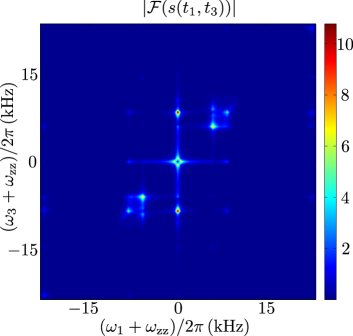
Figure 3: 2D spectrum due to the resonant third-order terms $H^{(3)}_{\rm res}$, Eq. (9), in the Coulomb potential. Simulation parameters are given in the main text. A strong peak at $\omega_{1}=\omega_{3}=-\omega_{\rm zz}$ was removed from the spectrum for clarity. Eigenvalues of $H^{(3)}_{\rm res}$ for low phonon numbers are identified and the effect of homogeneous broadening is clearly visible as broadening of the peaks in vertical and horizontal directions.

The resulting spectrum shown in Fig. 3 shows two bright peaks above and below the central peak, which correspond to pathways starting in the ground state. Their vertical coordinates are shifted by $\pm\sqrt{2}\Omega_{\rm T}$, the eigenvalues of $H^{(3)}_{\rm res}$ for the lowest levels showing coherent energy transfer between the two modes. All peak coordinates are shifted with respect to $-\omega_{\rm zz}$ by an eigenvalue of $H^{(3)}_{\rm res}$ or a linear combination thereof, from which further eigenvalues can be inferred sup_mat_g . Off-diagonal peaks, moreover, are an evidence of coherence transfer ernst_buch . The figure clearly shows homogeneous broadening of the peaks along the frequency axes due to the coupling to the thermal reservoirs. This illustrates how 2D spectroscopy allows for a distinction between homogeneous and inhomogeneous broadening, since the latter leads to broadening of the peaks along the diagonal as in Fig. 2.

In summary, we have shown how to extend 2D spectroscopy for the investigation of nonlinear dynamics of crystals of trapped ions. The method offers significant advantages: it does not produce any signal for purely harmonic evolution and it allows for the separation of signals which would appear superposed in a linear spectrum. It also facilitates the characterization of noise in the system: while effective static disorder gives rise to diagonal lines, dephasing and heating occuring during each experimental run manifest in broadening in the horizontal and vertical directions. Furthermore, the protocol does not require ground-state cooling, a feature which is particularly appealing for the study of large ion crystals. Note that it is well-known how to achieve significant reductions in the number of measurements required to obtain 2D spectra by employing techniques from the field of matrix completion matrix_completion . The 2D spectroscopy methods presented here form a versatile new diagnostic toolbox that may be applied well beyond the two case studies discussed here to cover all many-body models that may be realized in ion traps including spin models, structural dynamics of large ion crystals, and models in which spin and vibrational degrees of freedom are coupled.

Acknowledgements. The authors acknowledge discussions with U. Poschinger at early stages of the project and useful comments on the manuscript from M. Bruderer. This work was supported by the EU Integrating Project SIQS, the EU STREPs EQUAM and PAPETS, the Alexander von Humboldt Foundation and the ERC Synergy Grant BioQ.

I Supplemental Material to “Two-dimensional spectroscopy for the study of ion Coulomb crystals”

Contents

1. I Supplemental Material to “Two-dimensional spectroscopy for the study of ion Coulomb crystals”
2. A The motional Hamiltonian in the harmonic approximation
3. B Third-order terms in the Coulomb potential
4. C Fourth-order terms in the Coulomb potential
5. D Coherence transfer pathways and phase cycling
6. E Impact of phase fluctuations on phase cycling
7. F Cancellation of the signal from harmonic systems
8. G Identification of peaks in the third-order spectrum

Appendix A The motional Hamiltonian in the harmonic approximation

We start by considering $N$ singly charged atomic ions of mass $m$ confined in a linear Paul trap. We assume the trapping potential to be harmonic such that we can write

$$V_{\rm t}=\sum_{i=1}^{N}\sum_{\mu=x,y,z}\frac{1}{2}m\omega_{\mu}^{2}r_{i\mu}^{2}$$ (10)

where $\omega_{\mu}$ is the (pseudopotential) trapping frequency in spatial direction $\mu$ and $r_{i\mu}$ is the spatial coordinate $\mu$ of ion $i$. The Coulomb interaction between the ions is given by:

$$V_{\rm C}=\frac{1}{2}\sum_{i,j\neq i}\frac{e^{2}}{4\pi\epsilon_{0}}\frac{1}{|{\bf r}_{i}-{\bf r}_{j}|}$$ (11)

with $\epsilon_{0}$ the vacuum permittivity and $e$ the elementary charge. The full potential is then:

$$V=V_{\rm t}+V_{\rm C}.$$ (12)

Adding the kinetic energy of the ions we arrive at the full Hamiltonian for the motional degrees of freedom:

$$H=\sum_{i,\mu}\left(\frac{p_{i\mu}^{2}}{2m}+\frac{1}{2}m\omega_{\mu}^{2}r_{i\mu}^{2}\right)+\frac{1}{2}\sum_{i\neq j}\frac{e^{2}}{4\pi\epsilon_{0}}\frac{1}{|{\bf r}_{i}-{\bf r}_{j}|}.$$ (13)

Assuming the trap axis along the spatial $z$-direction and $\omega_{x},\>\omega_{y}\gg\omega_{z}$, the ions arrange on a string along $z$ and the radial equilibrium positions are given by $x_{i}^{0}=y_{i}^{0}=0$ while the axial equilibrium positions are determined by

$$\left.\frac{\partial V}{\partial z_{i}}\right|_{z_{i}^{0}}=0.$$ (14)

Introducing the charateristic length scale

$$l_{z}^{3}=\frac{e^{2}}{4\pi\epsilon_{0}m\omega_{z}^{2}}$$ (15)

the axial equilibrium positions $z_{i}^{0}$ may be written as

$$z_{i}^{0}=l_{z}u_{i}^{0}$$ (16)

where the $u_{i}^{0}$ are usually termed the dimensionless equilibrium positions of the ion string james_normal_modes_sm . Eq. (14) can then be written in terms of the $u_{i}^{0}$ which has the advantage that the result is independent of the specific ion mass and trapping frequency. The values of the $z_{i}^{0}$ for a specific setup are readily calculated with the help of $l_{z}$. A collection of the values of $u_{i}^{0}$ for up to ten ions may be found in james_normal_modes_sm . If the ions are sufficiently cold they perform only small excursions $\delta r_{j\mu}(t)$ around their equilibrium positions such that their spatial coordinates can be expressed as

$$r_{j\mu}(t)=r_{j\mu}^{0}+\delta r_{j\mu}(t).$$ (17)

Expanding the full potential in Eq. (12) to second order in these small displacements from equilibrium one obtains

$$V\simeq V^{(2)}=\frac{1}{2}\left.\sum_{i,j,\mu,\beta}\frac{\partial^{2}V}{\partial r_{i\mu}\partial r_{j\beta}}\right|_{{\bf r}_{i,j}^{0}}\delta r_{i\mu}\delta r_{j\beta}$$ (18)

where the constant energy shift due to the zeroth order contribution has been omitted. For a linear string of ions there are no couplings between the motion in different spatial directions in the second order approximation, so that the potential is given by

$$V^{(2)}=\frac{m\omega_{z}^{2}}{2}\sum_{i,j}\sum_{\mu}V^{\mu}_{ij}\delta r_{i\mu}\delta r_{j\mu}.$$ (19)

Before giving the expression for the $V^{\mu}_{ij}$ let us define the trap anisotropies

$$\alpha_{x/y}=\left(\frac{\omega_{z}}{\omega_{x/y}}\right)^{2}.$$ (20)

Note that small values of $\alpha_{x/y}$ imply that the confinement in the radial directions is much tighter than in the axial direction. With these definitions at hand we can write the Hessian matrices of the potential at the ions’ equilibrium positions as james_third_order_sm

$$V_{ij}^{z}=\begin{cases}1+2\sum_{p\neq j}\frac{1}{|u_{j}^{0}-u_{p}^{0}|^{3}}&{\rm if}\hskip 4.30554pti=j\\ \frac{-2}{|u_{j}^{0}-u_{i}^{0}|^{3}}&{\rm if}\hskip 4.30554pti\neq j\end{cases}$$ (21)

and

$$V_{ij}^{x/y}=\left(\frac{1}{\alpha_{x/y}}+\frac{1}{2}\right)\delta_{ij}-\frac{1}{2}V_{ij}^{z}.$$ (22)

Here, the $u_{i}^{0}$ are the dimensionless equilibrium positions defined in Eq. (16) and $\delta_{ij}$ is the Kronecker delta.

In the harmonic approximation the Hamiltonian Eq. (13) may be written as

$$H=\sum_{i,\mu}\frac{p_{i\mu}^{2}}{2m}+\frac{m\omega_{z}^{2}}{2}\sum_{i,j}\sum_{\mu}V^{\mu}_{ij}\delta r_{i\mu}\delta r_{j\mu}.$$ (23)

For each direction $\mu$, the matrix $V^{\mu}_{ij}$ is real and symmetric. As is apparent from Eqs. (21) and (22) all Hessians are diagonalized by the same orthogonal matrix $M$. The system is then described by $N$ uncoupled normal modes in every spatial direction goldstein . Physically, the entries $M_{jn}$ of the matrix can be understood as the normalized amplitude of normal mode $n$ at ion $j$ goldstein ; james_normal_modes_sm . Quantizing the motion according to

$$\begin{split}r_{j\mu}&=\sum_{n}M_{jn}\sqrt{\frac{\hbar}{2m\omega_{\mu,n}}}(a_{\mu,n}+a_{\mu,n}^{\dagger}),\\ p_{j\mu}&=\sum_{n}{\rm i}M_{jn}\sqrt{\frac{\hbar m\omega_{\mu,n}}{2}}(a_{\mu,n}^{\dagger}-a_{\mu,n})\end{split}$$ (24)

the Hamiltonian Eq. (23) can be cast into the form

$$H_{0}=\sum_{\mu,n}\hbar\omega_{\mu,n}a_{\mu,n}^{\dagger}a_{\mu,n}$$ (25)

which corresponds to Eq. (4) of the main text. Note that we have omitted the ground state energy. The axial normal mode frequencies are given by

$$\omega_{z,n}=\sqrt{\lambda_{n}^{z}}\omega_{z}$$ (26)

where $\omega_{z,n}$ is the frequency of mode $n$ and the $\lambda_{n}^{z}$ ($n=1,\dots,N$) are the eigenvalues of $V_{ij}^{z}$, ordered such that they increase with increasing $n$. Similarly, the radial normal mode frequencies read

$$\omega_{x/y,n}=\sqrt{\gamma_{n}^{x/y}}\omega_{z}$$ (27)

where the $\gamma_{n}^{x/y}$ are the eigenvalues of $V_{ij}^{x/y}$ which can be written as

$$\gamma_{n}^{x/y}=\frac{1}{\alpha_{x/y}}+\frac{1}{2}-\frac{\lambda_{n}^{z}}{2}.$$ (28)

Hence, the eigenvalues in the radial directions decrease with increasing $n$. Note, however, that the eigenvalues in the axial and radial directions with equal index $n$ correspond to the same eigenvector and thus the corresponding modes have the same structure. It can be shown james_normal_modes_sm that the smallest eigenvalue of $V_{ij}^{z}$ is $\lambda_{1}^{z}=1$ and corresponds to the center-of-mass mode. Thus, the center-of-mass mode is the energetically lowest lying mode in the axial direction while it is the energetically highest lying mode in the radial directions. Conversely, the energetically highest lying mode in the axial direction, corresponding to the eigenvalue $\lambda_{N}^{z}$, is the mode where neighboring ions perform out-of-phase oscillations. In the radial directions this mode is called the zigzag mode and is the energetically lowest lying mode. In Fig. 4 we schematically show all motional modes for a linear three-ion crystal.

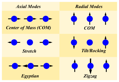
Figure 4: Sketch illustrating the different vibrational eigenmodes of a linear three-ion crystal and the standard naming convention for these modes. The inter-ion spacing is of the order of $l_{z}$.

Approaching the linear-to-zigzag structural transition the zigzag mode is particularly relevant as it is the soft mode in this transition for the case of infinitely many ions linear-zigzag_sm and numerical simulations show this behavior also emerges for chains of finite size. The instability of the linear chain below a critical value of the transverse confinement can be seen from Eq. (28). If the radial confinement is lowered in one direction, e.g. the $x$-direction, while the axial confinement is held constant, the value of $\alpha_{x}$ increases. Accordingly, the eigenvalues $\gamma_{n}^{x}$ become smaller and for a certain anisotropy $\alpha_{x}$ we have $\gamma_{N}^{x}=0$. Lowering the potential further would yield $\gamma_{N}^{x}<0$, an indicator that the linear configuration is not stable anymore. Indeed, in this parameter regime the ions break away from the linear configuration and arrange in a planar zigzag structure. This behavior is well-known and critical anisotropies have been estimated and experimentally tested for different numbers of ions linear-zigzag_experiment . In Fig. 5 we show the scaling of the eigenvalues and mode frequencies for the transverse modes in $x$-direction as a function of the trap anisotropy for a crystal of three ⁴⁰Ca⁺ ions and an axial trapping frequency $\omega_{z}/2\pi=2\,$MHz.

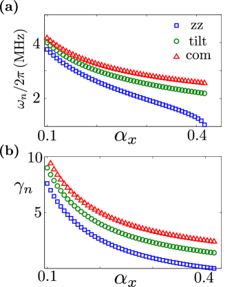
Figure 5: (a): Normal mode frequencies for a crystal of three ⁴⁰Ca⁺ ions as a function of the trap anisotropy $\alpha_{x}=(\omega_{z}/\omega_{x})^{2}$ for an axial trapping frequency $\omega_{z}/2\pi=2\,$MHz. (b): Eigenvalues of the Hessian in $x$-direction as a function of the trap anisotropy $\alpha_{x}$ for the same parameters as in (a).

Appendix B Third-order terms in the Coulomb potential

In Eq. (10) we have assumed that the trapping is harmonic which is a very good approximation in a Paul trap, unless nonlinearities are deliberately added to the trapping potential, e.g. by means of optical fields optical_potential . The next order corrections to the potential in Eq. (18) stem from the Coulomb interaction and are obtained by evaluating

$$V^{(3)}=\frac{1}{3!}\sum_{i,j,k\atop\mu,\beta,\gamma}\left.\frac{\partial^{3}V_{\rm C}}{\partial r_{k\gamma}\partial r_{i\mu}\partial r_{j\beta}}\right|_{{\bf r}_{i,j,k}^{0}}\delta r_{i\mu}\delta r_{j\beta}\delta r_{k\gamma}.$$ (29)

Inserting the dimensionless equilibrium positions from Eq. (16) into the above expression, after some algebra we obtain james_third_order_sm

$$V^{(3)}=\frac{m\omega_{z}^{2}}{2l_{z}}\sum_{i,j,k}C_{ijk}(3\delta x_{i}\delta x_{j}+3\delta y_{i}\delta y_{j}-2\delta z_{i}\delta z_{j})\delta z_{k}$$ (30)

with the tensor $C_{ijk}^{(3)}$

$$C^{(3)}_{ijk}=\begin{dcases}\sum_{p\neq k}\frac{{\rm sgn}(u_{k}^{0}-u_{p}^{0})}{|u_{k}^{0}-u_{p}^{0}|^{4}}&{\rm if}\>i=j=k\\ \frac{{\rm sgn}(u_{k}^{0}-u_{j}^{0})}{|u_{k}^{0}-u_{j}^{0}|^{4}}&{\rm if}\>i=j\neq k\\ \frac{{\rm sgn}(u_{i}^{0}-u_{k}^{0})}{|u_{i}^{0}-u_{k}^{0}|^{4}}&{\rm if}\>i\neq j=k\\ \frac{{\rm sgn}(u_{j}^{0}-u_{k}^{0})}{|u_{j}^{0}-u_{k}^{0}|^{4}}&{\rm if}\>i=k\neq j\\ 0&{\rm if}i\neq j\neq k.\\ \end{dcases}$$ (31)

Quantizing the coordinates according to Eq. (24) and using $a_{x,n}=a_{n},\>a_{y,n}=b_{n}$ and $a_{z,n}=c_{n}$ we arrive at the third-order correction Hamiltonian james_third_order_sm

$$\begin{split}H^{(3)}_{\rm full}=&\frac{z_{0}}{4l_{z}}\hbar\omega_{z}\sum_{n,m,p}D_{nmp}^{(3)}\times\\ &\left[\frac{3(a_{n}+a_{n}^{\dagger})(a_{m}+a_{m}^{\dagger})}{\sqrt[4]{\gamma_{n}^{x}\gamma_{m}^{x}}}+\frac{3(b_{n}+b_{n}^{\dagger})(b_{m}+b_{m}^{\dagger})}{\sqrt[4]{\gamma_{n}^{y}\gamma_{m}^{y}}}\right.\\ &\left.-\frac{2(c_{n}+c_{n}^{\dagger})(c_{m}+c_{m}^{\dagger})}{\sqrt[4]{\lambda_{n}^{z}\lambda_{m}^{z}}}\right]\frac{(c_{p}+c_{p}^{\dagger})}{\sqrt[4]{\lambda_{p}^{z}}}\\ \end{split}$$ (32)

where $D_{nmp}^{(3)}$ is defined as

$$D_{nmp}^{(3)}=\sum_{i,j,k}C_{ijk}^{(3)}M_{in}M_{jm}M_{kp}$$ (33)

and $z_{0}=\sqrt{\hbar/(2m\omega_{z})}$ is the spread of the longitudinal center-of-mass ground state wave packet. We note that all $D_{nmp}^{(3)}$ involving the center-of-mass modes, i.e. all $D_{nmp}^{(3)}$ with at least one index equal to one, vanish. Physically, this is due to the fact that transferring excitations to or from the center-of-mass modes would change the momentum of the crystal as a whole. This, however, cannot be due to the Coulomb interaction james_third_order_sm .

Transforming the quantized interaction Hamiltonian Eq. (32) to an interaction picture with respect to the time-independent Hamiltonian $H_{0}$, Eq. (25), it can be inspected for resonances. This has been done in detail in james_third_order_sm , where a list of possible resonances, i.e. involved modes and according values of $\alpha_{x/y}$, is provided for up to $N=10$ ions. Two types of resonances can occur: a radial phonon is created while one longitudinal and one radial phonon are annihilated or two transverse phonons are created upon the annihilation of one longitudinal phonon. Considering the case of $N=3$ ions only the latter resonance is possible. For our simulations we assumed that the degeneracy between the radial modes is lifted such that a resonance involves only one radial mode and the other mode is sufficiently far off-resonant. We chose to consider the $x$-direction for the transverse modes. For $\alpha_{x}=20/63$ one obtains a resonant coupling between the $x$-zigzag mode and the stretch mode. In this case the resonant part of the Hamiltonian in Eq. (32) reads

$$H_{\rm res}^{(3)}=3\frac{z_{0}}{4l_{z}}\hbar\omega_{z}\frac{D_{332}^{(3)}}{\sqrt[4]{\gamma_{3}^{x}\gamma_{3}^{x}\lambda_{2}^{z}}}\left[a_{3}^{2}c_{2}^{\dagger}+(a_{3}^{\dagger})^{2}c_{2}\right].$$ (34)

Setting $\Omega_{\rm T}=3z_{0}\omega_{z}D_{332}^{(3)}/(4l_{z}\sqrt[4]{\gamma_{3}^{x}\gamma_{3}^{x}\lambda_{2}^{z}})$ as well as $a_{3}=a_{\rm zz},\>c_{2}=c_{\rm str}$ we recover Eq. (9) of the main text.

Appendix C Fourth-order terms in the Coulomb potential

The fourth-order corrections to the potential in Eq. (18) due to the Coulomb potential are obtained by evaluating the expression

$$V^{(4)}=\frac{1}{4!}\sum_{i,j,k,l\atop\mu,\beta,\gamma,\delta}\left.\frac{\partial^{4}V_{\rm C}}{\partial r_{l\delta}\partial r_{k\gamma}\partial r_{i\mu}\partial r_{j\beta}}\right|_{{\bf r}_{i,j,k,l}^{0}}\delta r_{i\mu}\delta r_{j\beta}\delta r_{k\gamma}\delta r_{l\delta}.$$ (35)

After a rather lengthy but straightforward calculation we arrive at

$$\begin{split}V^{(4)}=&\frac{1}{4!}\frac{3e^{2}}{4\pi\epsilon_{0}}\frac{1}{l_{z}^{5}}\sum_{i,j,k,l}C_{ijkl}^{(4)}\left[3\delta x_{i}\delta x_{j}\delta x_{k}\delta x_{l}\right.\\ &+3\delta y_{i}\delta y_{j}\delta y_{k}\delta y_{l}+8\delta z_{i}\delta z_{j}\delta z_{k}\delta z_{l}+6\delta x_{i}\delta x_{j}\delta y_{k}\delta y_{l}\\ &\left.-24\delta x_{i}\delta x_{j}\delta z_{k}\delta z_{l}-24\delta y_{i}\delta y_{j}\delta z_{k}\delta z_{l}\right]\end{split}$$ (36)

where

$$\begin{split}C_{ijkl}^{(4)}=\delta_{ij}\delta_{jk}\delta_{kl}\sum_{p\neq l}\frac{1}{|u_{l}^{0}-u_{p}^{0}|^{5}}+\delta_{ij}\delta_{jk}(1-\delta_{kl})\frac{-1}{|u_{k}^{0}-u_{l}^{0}|^{5}}\\ +\delta_{ij}(1-\delta_{jk})\delta_{lj}\frac{-1}{|u_{l}^{0}-u_{k}^{0}|^{5}}+(1-\delta_{ij})\delta_{jk}\delta_{kl}\frac{-1}{|u_{l}^{0}-u_{i}^{0}|^{5}}\\ +(1-\delta_{ij})\delta_{ik}\delta_{kl}\frac{-1}{|u_{j}^{0}-u_{l}^{0}|^{5}}+\delta_{ij}(1-\delta_{jk})\delta_{kl}\frac{1}{|u_{j}^{0}-u_{l}^{0}|^{5}}\\ +(1-\delta_{ij})\delta_{jk}\delta_{il}\frac{1}{|u_{k}^{0}-u_{l}^{0}|^{5}}+(1-\delta_{ij})\delta_{ik}\delta_{jl}\frac{1}{|u_{l}^{0}-u_{k}^{0}|^{5}}\end{split}$$ (37)

or

$$C_{ijkl}^{(4)}=\begin{dcases}\sum_{p\neq l}\frac{1}{|u_{l}^{0}-u_{p}^{0}|^{5}}&{\rm if}\>\>i=j=k=l\\ \frac{-1}{|u_{k}^{0}-u_{l}^{0}|^{5}}&{\rm if}\>\>i=j=k\neq l\\ \frac{1}{|u_{j}^{0}-u_{l}^{0}|^{5}}&{\rm if}\>\>i=j\neq k=l\\ 0&{\rm else.}\end{dcases}$$ (38)

The indices of $C_{ijkl}^{(4)}$ can be interchanged at will. Thus, the above definition covers all entries of the tensor. Using Eq. (24) we obtain the quantized form of the fourth-order expansion of the Coulomb potential. The calculation is straightforward and yields

$$\begin{split}&H_{\rm full}^{(4)}=\left(\frac{z_{0}}{4l_{z}}\right)^{2}\hbar\omega_{z}\sum_{n,m,p,q}D_{nmpq}^{(4)}\times\\ &\left[\frac{3}{\sqrt[4]{\gamma_{n}^{x}\gamma_{m}^{x}\gamma_{p}^{x}\gamma_{q}^{x}}}(a_{n}+a_{n}^{\dagger})(a_{m}+a_{m}^{\dagger})(a_{p}+a_{p}^{\dagger})(a_{q}+a_{q}^{\dagger})\right.\\ &+\frac{3}{\sqrt[4]{\gamma_{n}^{y}\gamma_{m}^{y}\gamma_{p}^{y}\gamma_{q}^{y}}}(b_{n}+b_{n}^{\dagger})(b_{m}+b_{m}^{\dagger})(b_{p}+b_{p}^{\dagger})(b_{q}+b_{q}^{\dagger})\\ &+\frac{8}{\sqrt[4]{\lambda_{n}^{z}\lambda_{m}^{z}\lambda_{p}^{z}\lambda_{q}^{z}}}(c_{n}+c_{n}^{\dagger})(c_{m}+c_{m}^{\dagger})(c_{p}+c_{p}^{\dagger})(c_{q}+c_{q}^{\dagger})\\ &+\frac{6}{\sqrt[4]{\gamma_{n}^{x}\gamma_{m}^{x}\gamma_{p}^{y}\gamma_{q}^{y}}}(a_{n}+a_{n}^{\dagger})(a_{m}+a_{m}^{\dagger})(b_{p}+b_{p}^{\dagger})(b_{q}+b_{q}^{\dagger})\\ &-\frac{24}{\sqrt[4]{\gamma_{n}^{x}\gamma_{m}^{x}\lambda_{p}^{z}\lambda_{q}^{z}}}(a_{n}+a_{n}^{\dagger})(a_{m}+a_{m}^{\dagger})(c_{p}+c_{p}^{\dagger})(c_{q}+c_{q}^{\dagger})\\ &\left.-\frac{24}{\sqrt[4]{\gamma_{n}^{y}\gamma_{m}^{y}\lambda_{p}^{z}\lambda_{q}^{z}}}(b_{n}+b_{n}^{\dagger})(b_{m}+b_{m}^{\dagger})(c_{p}+c_{p}^{\dagger})(c_{q}+c_{q}^{\dagger})\right]\end{split}$$ (39)

where we have introduced

$$D_{nmpq}^{(4)}=\sum_{i,j,k,l}C_{ijkl}^{(4)}M_{in}M_{jm}M_{kp}M_{lq}.$$ (40)

Again, there are no couplings to the center-of-mass modes. This can be shown following the proof for the third order in Ref. james_third_order_sm . We start by realizing that

$$\sum_{l}C_{ijkl}^{(4)}=0.$$ (41)

This can be seen in the following way: if $i\neq j\neq k$ all terms in the above sum are zero and the result is trivial; if $i=j\neq k$ we have $\sum_{l}C_{iikl}^{(4)}=C_{iiki}^{(4)}+C_{iikk}^{(4)}=0$ as $C_{iiki}^{(4)}=-C_{iikk}^{(4)}$ from the definition in Eq. (38); in case $i=j=k$ we have $\sum_{l}C_{iiil}^{(4)}=C_{iiii}^{(4)}+\sum_{l\neq i}C_{iiil}^{(4)}$ which is again found to be zero by using Eq. (38). Using that $M_{l1}=1/\sqrt{N},\>l=1,\dots,N$ we obtain

$$\begin{split}D_{nmp1}^{(4)}&=\sum_{i,j,k,l}C_{ijkl}^{(4)}M_{in}M_{jm}M_{kp}\frac{1}{\sqrt{N}}\\ &=\frac{1}{\sqrt{N}}\sum_{i,j,k}M_{in}M_{jm}M_{kp}\sum_{l}C_{ijkl}^{(4)}=0.\end{split}$$ (42)

As the indices of $C_{ijkl}^{(4)}$ can be interchanged freely this is true for every element of $D_{nmpq}^{(4)}$ with at least one index equal to 1.

Let us now identify the regimes in which the fourth-order terms in the Hamiltonian, Eq. (39), have appreciable contributions to the motional dynamics. Under normal trapping conditions ($\omega_{x},\omega_{y}\gg\omega_{z}$) the corrections to the harmonic Hamiltonian, Eq. (25), are very small due to the prefactor $[z_{0}/(4l_{z})]^{2}\approx 10^{-6}$. For instance, in innsbruck_cross_kerr_sm Kerr-type interactions due to the fourth-order terms of the Coulomb potential were found to have strengths $\sim 1-10\,$Hz. The situation is different approaching the linear-to-zigzag transition. If the trapping potential in $x$-direction is relaxed reaching the close vicinity of the structural transition, $\gamma_{N}^{x}$ approaches zero while all other eigenvalues have values well above zero (cf. Fig. 5 for the case of three ions). Hence, due to the appearance of $\gamma_{N}^{x}$ in the denominator, the terms involving $\gamma_{N}^{x}$ acquire an appreciable value. Retaining only terms involving modes in the $x$-direction in Eq. (39) yields the Hamiltonian in Eq. (6) of the main text.

Table 2: Shifts in the normal mode frequencies due to fourth-order effects of the Coulomb interaction for a crystal of $N=3$ ions with $\omega_{\rm z}/2\pi=2\,{\rm MHz}$ and $\omega_{\rm x}/2\pi=3.1012\,{\rm MHz},\>\omega_{\rm y}/2\pi=5\,{\rm MHz}$

Frequency shift	$\Delta\omega_{\rm x,2}/2\pi$	$\Delta\omega_{\rm zz}/2\pi$	$\Delta\omega_{\rm y,2}/2\pi$	$\Delta\omega_{\rm y,3}/2\pi$	$\Delta\omega_{\rm z,2}/2\pi$	$\Delta\omega_{\rm z,3}/2\pi$
Third order	-0.5008 kHz	-10.0850  kHz	0 kHz	0 kHz	0.5275  kHz	0.2821  kHz
Fourth order	0.4791 kHz	25.2874 kHz	0.0826 kHz	0.2894 kHz	-0.4371 kHz	-0.9430 kHz
Effective	-0.0217 kHz	15.2025 kHz	0.0826 kHz	0.2894 kHz	0.0905 kHz	-0.6609 kHz

Table 3: Dephasing rates due to fourth-order effects of the Coulomb interaction for a crystal of $N=3$ ions with $\omega_{\rm z}/2\pi=2\,{\rm MHz}$ and $\omega_{\rm x}/2\pi=3.1012\,{\rm MHz},\>\omega_{\rm y}/2\pi=5\,{\rm MHz}$

	$\Omega_{\rm d,2}^{x}/2\pi$	$(\Omega_{\rm SI}/2)/2\pi$	$\Omega_{\rm d,2}^{y}/2\pi$	$\Omega_{\rm d,3}^{y}/2\pi$	$\Omega_{\rm d,2}^{z}/2\pi$	$\Omega_{\rm d,3}^{z}/2\pi$
Third order	-1.0487 kHz	-10.3467 kHz	0 kHz	0 kHz	1.0551 kHz	0.5171 kHz
Fourth order	0.9582 kHz	12.9082 kHz	0.1652 kHz	0.5787 kHz	-0.8741 kHz	-1.8860 kHz
Effective	-0.0905 kHz	2.5615 kHz	0.1652 kHz	0.5787 kHz	0.1810 kHz	-1.3690 kHz

This Hamiltonian has to be considered in more detail in order to identify the contributions relevant for the dynamics. To facilitate the analysis we divide the Hamiltonian in Eq. (6) of the main text into three parts $H^{(4)}=H_{\rm xx}+H_{\rm xy}+H_{\rm xz}$ where the indices denote the spatial direction in which the first and last two pairs of operators act. We restrict our analysis to the case of $N=3$ ions; the generalization to larger $N$ is straightforward. The first term reads

$$\begin{split}H_{\rm xx}=&3\left(\frac{z_{0}}{4l_{z}}\right)^{2}\hbar\omega_{z}\sum_{n,m,p,q}\frac{D_{nmpq}^{(4)}}{\sqrt[4]{\gamma_{n}^{x}\gamma_{m}^{x}\gamma_{p}^{x}\gamma_{q}^{x}}}\times\\ &(a_{n}+a_{n}^{\dagger})(a_{m}+a_{m}^{\dagger})(a_{p}+a_{p}^{\dagger})(a_{q}+a_{q}^{\dagger}).\end{split}$$ (43)

Moving to a frame rotating with the phonon frequencies we can find the resonant terms which will contribute appreciably to the dynamics. The Hamiltonian contains many Kerr-type terms $a_{n}^{\dagger}a_{n}a_{m}^{\dagger}a_{m}$ (and permutations thereof) coupling two modes $n$ and $m$. These terms do not acquire a time dependence in the rotating frame. In the special case $m=n$ these terms can be written as $(a_{n}^{\dagger})^{2}a_{n}^{2}+a_{n}^{\dagger}a_{n}$. Thus, the non-rotating fourth-order terms lead to Kerr-type couplings between different modes and also to a self-interaction of the modes together with a shift of the mode frequencies. In order to make sure that only these non-rotating terms are the dominant contribution to the dynamics one needs to check if the time-dependent terms can be neglected in a RWA. To this end we assume realistic experimental parameters as summarized in Table I of the main text and perform a quantitative anlysis: For each combination $nmpq$ there are 16 operator terms $O_{nmpq,i},\>i=1,\dots,16$, whose coefficients and frequencies we denote by $c_{nmpq,i}$ and $\omega_{nmpq,i}$, respectively. Then, we check if $c_{nmpq,i}/\omega_{nmpq,i}\ll 1$ for all energy non-conserving terms where $\omega_{nmpq,i}\neq 0$. This analysis shows that the energy non-conserving terms can be neglected in a RWA. Finally, ordering the resonant terms yields

$$\begin{split}H_{\rm xx}=&\frac{\hbar\Omega_{\rm SI}}{2}(a_{\rm zz}^{\dagger})^{2}a_{\rm zz}^{2}+\hbar\Delta\omega_{{\rm zz}}a_{\rm zz}^{\dagger}a_{\rm zz}\\ &+\hbar\Omega_{\rm d,2}^{x}a_{\rm zz}^{\dagger}a_{\rm zz}a^{\dagger}_{2}a_{2}+\hbar\Delta\omega_{x,2}a^{\dagger}_{2}a_{2}\end{split}$$ (44)

where

$$\begin{split}\Omega_{\rm SI}&=12\times 3\left(\frac{z_{0}}{4l_{z}}\right)^{2}\frac{D_{3333}^{(4)}}{\gamma_{\rm zz}^{x}}\omega_{z},\\ \Omega_{\rm d,2}^{x}&=24\times 3\left(\frac{z_{0}}{4l_{z}}\right)^{2}\frac{D_{2233}^{(4)}}{\sqrt{\gamma_{2}^{x}\gamma_{\rm zz}^{x}}}\omega_{z},\\ \Delta\omega_{\rm zz}&=\Omega_{\rm SI}+\frac{1}{2}\Omega_{\rm d,2}^{x},\\ \Delta\omega_{x,2}&=\frac{1}{2}\Omega_{\rm d,2}^{x}\\ \end{split}$$ (45)

and we use the index zz (instead of 3) to denote the $x$ zigzag mode. Note the we omitted the self-interaction of the $x$ tilt mode as it does not involve $\gamma_{\rm zz}^{x}$. Numerical values for the frequency shifts and mode couplings for the parameters used in our simulations can be found in Tables 2 and 3.

Following the same procedure we obtain

$$H_{\rm xy}=a_{\rm zz}^{\dagger}a_{\rm zz}\left(\hbar\Delta\omega_{\rm zz}^{\prime}+\sum_{n=2,3}\hbar\Omega_{\rm d,n}^{y}b_{n}^{\dagger}b_{n}\right)+\sum_{n=2,3}\hbar\Delta\omega_{y,n}b_{n}^{\dagger}b_{n}$$ (46)

where

$$\begin{split}\Omega_{\rm d,2}^{y}&=4\times 6\left(\frac{z_{0}}{4l_{z}}\right)^{2}\frac{D_{3322}^{(4)}}{\sqrt{\gamma_{\rm zz}^{x}\gamma_{2}^{y}}}\omega_{z},\\ \Omega_{\rm d,3}^{y}&=4\times 6\left(\frac{z_{0}}{4l_{z}}\right)^{2}\frac{D_{3333}^{(4)}}{\sqrt{\gamma_{\rm zz}^{x}\gamma_{3}^{y}}}\omega_{z},\\ \Delta\omega_{\rm zz}^{\prime}&=\frac{1}{2}(\Omega_{\rm d,2}^{y}+\Omega_{\rm d,3}^{y}),\\ \Delta\omega_{y,n}&=\frac{\Omega_{\rm d,n}^{y}}{2}.\\ \end{split}$$ (47)

Again numerical values can be found in Tables 2 and 3. Note that the frequency shift of the $x$ zigzag mode given in Table 2 is the sum of the shifts in Eqs. (44), (46) and (48). The resonant contributions of the third part are given by

$$H_{\rm xz}=a_{\rm zz}^{\dagger}a_{\rm zz}\left(\hbar\Delta\omega_{\rm zz}^{\prime\prime}+\sum_{n=2,3}\hbar\Omega_{\rm d,n}^{z}c_{n}^{\dagger}c_{n}\right)+\sum_{n=2,3}\hbar\Delta\omega_{z,n}c_{n}^{\dagger}c_{n}$$ (48)

where the mode couplings $\Omega_{\rm d,n}^{z}$ and the frequency shifts $\Delta\omega_{z,n}$ are defined analogous as in Eq. (47). Considering the numerical values for the mode couplings and frequency shifts in Tables 2 and 3 we realize that, except for the $x$ zigzag mode, the frequency shifts are much smaller than the motional frequencies which are of the order of MHz. Therefore, we neglect the frequency shifts for all modes except the zigzag mode. The sum of the above Hamiltonians $H^{(4)}=H_{\rm xx}+H_{\rm xy}+H_{\rm xz}$ then yields the structure of the Hamiltonian $H_{\rm eff}^{(4)}$ in Eqs. (7) and (8) of the main text. Let us emphasize that the self-interaction and frequency shift of the zigzag mode increase fastest when approaching the structural transition, scaling as $1/\gamma_{\rm zz}^{x}$, while the mode couplings only scale as $1/\sqrt{\gamma_{\rm zz}^{x}}$ (cf. Eqs. (45) and (47)).

An analysis including only the fourth-order terms is incomplete, since the off-resonant third-order Hamiltonian terms induce energy shifts of the same order of magnitude as the fourth-order terms, leading to corrections for the self-interactions, frequency shifts and dephasing rates innsbruck_cross_kerr_sm ; NRJ_2009_sm . For our purposes we only need to consider the part of the Hamiltonian $H^{(3)}_{\rm full}$, Eq. (32), involving $x$ modes, namely

$$\begin{split}H^{(3)}_{\rm x}=&3\frac{z_{0}}{4l_{z}}\hbar\omega_{z}\sum_{n,m,p}\frac{D_{nmp}^{(3)}}{\sqrt[4]{\gamma_{n}^{x}\gamma_{m}^{x}\lambda_{p}^{z}}}\times\\ &(a_{n}+a_{n}^{\dagger})(a_{m}+a_{m}^{\dagger})(c_{p}+c_{p}^{\dagger}).\end{split}$$ (49)

Hence, the off-resonant energy shifts induced by third-order terms are obtained from

$$\Delta E=\sum_{\{n^{\prime}\}\neq\{n\}}\frac{|\langle\{n^{\prime}\}|H^{(3)}_{\rm x}|\{n\}\rangle|^{2}}{E_{n}-E_{n^{\prime}}}$$ (50)

where $|\{n\}\rangle$ is a motional Fock state with energy $E_{n}$ and $|\{n^{\prime}\}\rangle$ is any other motional Fock state with energy $E_{n^{\prime}}$. Realizing that $D^{(3)}_{233},\>D^{(3)}_{323}$ and $D^{(3)}_{332}$ are the only non-zero elements of $D^{(3)}_{nmp}$ involving the $x$ zigzag mode means that only states that differ in the quantum numbers $n_{\rm x,2},n_{\rm x,3},n_{\rm z,2},n_{\rm z,3}=n_{\rm t},n_{\rm zz},n_{\rm str},n_{\rm eg}$ are coupled and contribute to the energy shifts. More precisely, one finds that the state $|\{n\}\rangle=|n_{\rm t},n_{\rm zz},n_{\rm str},n_{\rm eg}\rangle$ is coupled to the states $|\{n^{\prime}\}\rangle=|n_{\rm t}\pm 1,n_{\rm zz}\pm 1,n_{\rm str},n_{\rm eg}\pm 1\rangle$, $|\{n^{\prime}\}\rangle=|n_{\rm t},n_{\rm zz}\pm 2,n_{\rm str}\pm 1,n_{\rm eg}\rangle$ and $|\{n^{\prime}\}\rangle=|n_{\rm t},n_{\rm zz},n_{\rm str}\pm 1,n_{\rm eg}\rangle$ by $H^{(3)}_{\rm x}$. Note that in the states where various “$\pm$” appear all possible combinations of plus and minus signs are relevant. The numerical values for the coupling rates and frequency shifts obtained from Eq. (50) are summarized in Tables 2 and 3.

Finally, the effective coupling rates and frequency shifts are obtained by summing the third- and fourth-order contributions and can be found in the last rows of Tables 2 and 3. The relative frequency shifts due to higher-order corrections of the Coulomb potential are $10^{-4}$ or smaller for all modes except the $x$ zigzag mode and are therefore neglected for these modes. From Eqs. (46) and (48) we see that a thermal occupation of the $y$ and $z$ modes, with the exception of the center-of-mass modes, causes shifts of the $x$ zigzag mode frequency and leads to effective dephasing. Therefore, we refer to the mode couplings $\Omega_{\rm d,n}^{\mu}$ also as dephasing rates. The numbers in Table 3 show that the coupling of the $x$ zigzag mode to other modes is strongest for the $y$ zigzag and the Egyptian mode. Accordingly, a thermal population of these modes yields the strongest contribution to the effective dephasing of the $x$ zigzag mode. The other dephasing contributions are considerably smaller. Combining these considerations with Eqs. (44), (46) and (48) we arrive at the effective Hamiltonian used for the simulations presented in the main text

$$\begin{split}H_{\rm eff}^{(4)}=&\frac{\hbar\Omega_{\rm SI}}{2}(a^{\dagger}_{\rm zz})^{2}a_{\rm zz}^{2}+\hbar\Delta\omega_{\rm zz}a_{\rm zz}^{\dagger}a_{\rm zz}\\ &+a_{\rm zz}^{\dagger}a_{\rm zz}\left(\hbar\Omega_{\rm d,3}^{y}b_{3}^{\dagger}b_{3}+\hbar\Omega_{\rm d,3}^{z}c_{3}^{\dagger}c_{3}\right).\end{split}$$ (51)

Appendix D Coherence transfer pathways and phase cycling

In this section we briefly summarize the ideas of coherence transfer pathways and phase cycling ernst which provide a means of postselecting only a certain set of contributions to the signal measured in a 2D experiment. We follow the treatment in ernst . Let us consider the simplest 2D experiment with trapped ions following the scheme introduced in the main text consisting of two displacement pulses followed by free evolutions. The time-evolution operator reads

$$U_{0}(t_{1},t_{2})=U_{\rm free}(t_{2})D(\alpha_{2})U_{\rm free}(t_{1})D(\alpha_{1}).$$ (52)

The concept of coherence transfer pathways in this context is the following: each of the displacements is written as a Taylor series in powers of $\alpha_{k}$ and we pick only one operator term acting on the density matrix from each side for each displacement. Every possible combination of these terms forms a coherence transfer pathway. However, only pathways that end up in a population contribute to the measured signal. A simple example of a pathway for an experiment described by the sequence in Eq. (52) is illustrated in Fig. 6 (a).

Figure 6: (a): A coherence transfer pathway for the simplest pulse sequence, Eq. (52), yielding a two-dimensional spectrum in our setup. The population $|n\rangle\langle n|$ is transferred to the observable population $|n+1\rangle\langle n+1|$. The phase $-\phi_{2}$ is imprinted on the final population. (b): A coherence transfer pathway for an experiment consisting of four displacements and two free evolutions is shown. The phase signature $\phi_{2}-\phi_{3}-\phi_{4}$ is imprinted onto the final population.

In the illustrated sequence, the first displacement sets a phase reference such that all subsequent displacements can be applied with well-defined phase, in this case $\alpha_{2}=|\alpha_{2}|{\rm e}^{{\rm i}\phi_{2}}$. The phase of the second displacement is “imprinted” on the final state; for example, the contribution to the signal from the pathway shown in Fig. 6 (a) is proportional to ${\rm e}^{-{\rm i}\phi_{2}}$ and therefore we say it carries a phase signature $-\phi_{2}$. There are other pathways with different phases that also end in a diagonal matrix element. The observable we measure in the end is the mode population $\langle a^{\dagger}a\rangle=\langle\hat{n}\rangle$. If $c_{n}$ is the probability of state $|n\rangle$ in the final state of the experiment, the signal is given by

$$\begin{split}s(t_{1},t_{2},\phi_{2})&=\langle\hat{n}\rangle=\sum_{n}c_{n}n=\sum_{n}n\sum_{p}c_{n,p}{\rm e}^{{\rm i}p\phi_{2}}\\ &=\sum_{p}{\rm e}^{{\rm i}p\phi_{2}}\sum_{n}c_{n,p}n=\sum_{p}s_{p}(t_{1},t_{2}){\rm e}^{{\rm i}p\phi_{2}}.\end{split}$$ (53)

For future reference we summarize the above equation to

$$s(t_{1},t_{2},\phi_{2})=\sum_{p}s_{p}(t_{1},t_{2}){\rm e}^{{\rm i}p\phi_{2}}.$$ (54)

Note that the result is a real number. We now want to obtain the contribution to the signal due to pathways like the one illustrated in Fig. 6 (a). This means we need to obtain the contribution to the signal carrying the phase signature $q\phi_{2}$ where $q=-1$. In order to achieve this, one performs $N_{\phi_{2}}$ experiments varying the phase $\phi_{2}$ systematically as

$$\phi_{2,k}=k\frac{2\pi}{N_{\phi_{2}}},\hskip 8.61108ptk=0,\dots,N_{\phi_{2}}-1.$$ (55)

The signal obtained from each of these experiments is made up of a superposition as in Eq. (54). Thus, we can obtain the contribution that stems from the pathways with the phase signature $-\phi_{2}$ by a discrete Fourier analysis of the signal obtained in the $N_{\phi_{2}}$ experiments

$$\begin{split}s(t_{1},t_{2},q)&=\frac{1}{N_{\phi_{2}}}\sum_{k=0}^{N_{\phi_{2}}-1}s(t_{1},t_{2},\phi_{2,k}){\rm e}^{-{\rm i}q\phi_{2,k}}\\ &=\frac{1}{N_{\phi_{2}}}\sum_{k=0}^{N_{\phi_{2}}-1}\left[\sum_{p}s_{p}(t_{1},t_{2}){\rm e}^{{\rm i}p\phi_{2,k}}\right]{\rm e}^{-{\rm i}q\phi_{2,k}}.\end{split}$$ (56)

This procedure is called phase cycling.

However, in this way one does not only obtain the contribution with the phase factor $q\phi_{2}$ but also all contributions with $(q+rN_{\phi_{2}})\phi_{2}$ where $r\in\mathbb{Z}$. Thus, after phase cycling the signal is made up of all selected contributions

$$s(t_{1},t_{2},q)=s_{q}(t_{1},t_{2})+\sum_{r}s_{q+rN_{\phi_{2}}}(t_{1},t_{2}).$$ (57)

The unwanted but selected contributions in the second part of Eq. (57) are due to terms of higher orders in the $\alpha_{i}$ in the expansion of the displacements. Hence, one must choose $|\alpha_{i}|$ sufficiently small so that only the first few terms of the Taylor expansion are non-negligible. Then, for large enough $N_{\phi_{2}}$ only the desired pathway contributes to the signal. This defines what we mean by a “small” displacement for a given $N_{\phi_{2}}$. Note that phase cycling requires an increase in the number of experiments performed by a factor $N_{\phi_{2}}$.

This procedure can be generalized to more than one phase. In Fig. 6 (b) we illustrate a pathway for a sequence of four displacements interleaved by two free evolutions as in the experiments proposed in the main text. The full time evolution operator then reads

$$U_{0}(t_{1},t_{3})=D(\alpha_{4})U_{\rm free}(t_{3})D(\alpha_{3})D(\alpha_{2})U_{\rm free}(t_{1})D(\alpha_{1})$$ (58)

where we have also set $t_{2}=t_{4}=0$. Here we can write

$$\alpha_{i}=|\alpha_{i}|{\rm e}^{{\rm i}\phi_{i}}$$ (59)

for $i\geq 2$. In the case illustrated in Fig. 6 (b) the phase $\phi_{2}-\phi_{3}-\phi_{4}$ is imprinted on the final population $|n+1\rangle\langle n+1|$. If we are interested in selecting the pathways with this phase signature we can perform phase cycling for each of these phases performing $N_{\phi_{i}}$ experiments for each phase. Defining ${\bf q}=(q_{2},q_{3},q_{4})=(1,-1,-1)$ and $\phi_{\bf k}=(\phi_{2,k_{2}},\phi_{3,k_{3}},\phi_{4,k_{4}})$ we obtain the desired signal through

$$s(t_{1},t_{3},{\bf q})=\frac{1}{N_{\rm tot}}\sum_{k_{2}}\sum_{k_{3}}\sum_{k_{4}}s(t_{1},t_{3},\phi_{\bf k}){\rm e}^{-{\rm i}{\bf q}\cdot\phi_{\bf k}}$$ (60)

where $N_{\rm tot}=N_{\phi_{2}}\cdot N_{\phi_{3}}\cdot N_{\phi_{4}}$. Note that this increases the number of experiments one needs to perform by a factor $N_{\rm tot}$.

Appendix E Impact of phase fluctuations on phase cycling

In the previous section it was shown how to select only a certain set of contributions to the signal of a 2D spectroscopy experiment by means of phase cycling. Phase cycling relies on the ability to apply a series of displacements on the considered motional mode with well-defined phases. So far, we have assumed that these phases can be controlled arbitrarily well. Yet, this is not true in a real experiment. In fact, in any real experiment the phases of the applied displacement pulses will be subject to fluctuations. In the following we shall analyze how these phase fluctuations affect the signal obtained in a 2D spectroscopy experiment. We will consider that the displacements are implemented by a state-dependent optical dipole force on the ions induced by laser radiation monroe_science_sm .

We start by considering the simplest case of an experiment involving only two displacements as described in the first part of the previous section. In this case the signal is ideally given by (see Eq. (54))

$$s(t_{1},t_{2},\phi_{2})=\sum_{p}s_{p}(t_{1},t_{2}){\rm e}^{{\rm i}p\phi_{2}}.$$ (61)

In practice, however, the signal considered in the above equation is the mean obtained from a series of experiments. In every experimental run the phase of the second pulse is subject to some small fluctuations about the desired value such that the phase $\phi_{2}$ becomes a random variable. Hence, Eq. (61) becomes

$$s(t_{1},t_{2},\phi_{2})=\sum_{p}\langle s_{p}(t_{1},t_{2}){\rm e}^{{\rm i}p\phi_{2}}\rangle_{\rm st}$$ (62)

where $\langle\dots\rangle_{\rm st}$ denotes the stochastic average. We are interested in the impact of phase fluctuations on the signal with a certain phase signature $q\phi_{2}$. Therefore, we want to compute the corrections to the signal $s(t_{1},t_{2},\phi_{2})$ caused by the fluctuating phase. We start by noting that the $s_{p}(t_{1},t_{2})$ are independent of the phase $\phi_{2}$ (see Eq. (53)). Further, we assume that for the $m$th experimental run we can write $\phi_{2,m}=\phi_{2}+\Delta\phi_{2,m}$ where $|\Delta\phi_{2,m}|\ll 1$, i.e. that the phase fluctuations are small on the considered timescale. This seems justified in light of the results of phase_fluctuations_fsk . There it was found that laser phase drifts of $2\pi$ occured on a timescale $\tau_{\rm d}\approx 10\,$s while the experiments we consider take place on a timescale $\tau_{\rm exp}\approx 5\,$ms. We can then write  Eq. (62) as

$$s(t_{1},t_{2},\phi_{2})=\sum_{p}{\rm e}^{{\rm i}p\phi_{2}}s_{p}(t_{1},t_{2})\langle{\rm e}^{{\rm i}p\Delta\phi_{2,m}}\rangle_{\rm st}.$$ (63)

In order to proceed we assume that the laser phase drifts can be modeled as a Wiener process stochastic_processes_gillespie . A Wiener process $X(t)$ is a Gaussian process that obeys the stochastic differential equation

$$\frac{{\rm d}X(t)}{{\rm d}t}=\sqrt{c}\Gamma(t)$$ (64)

where $c>0$ and $\Gamma(t)$ is Gaussian white noise. $X(t)$ is characterized by its initial value $X(t_{0})$ and the diffusion constant $c$. Its first and second moments read

$$\langle X(t)\rangle=X(0),\hskip 8.61108pt{\rm Var}[X(t)]=ct$$ (65)

where have set the initial time $t_{0}=0$. The covariance of the Wiener process for two times $s,t$ is given by breuer_petruccione

$${\rm Cov}[X(s),X(t)]=c\cdot{\rm min}(s,t).$$ (66)

For the phase fluctuations we assume a Wiener process with zero mean and diffusion constant $c=(4\pi^{2}/10)\cdot{\rm s}^{-1}$. We determine $c$ by identifying the standard deviation of the process at $t=10\,$s with $2\pi$. $\Delta\phi_{2,m}$ is then given by the value of the stochastic process at the instance of time when the second laser pulse is applied. Using $|\Delta\phi_{2,m}|\ll 1$ we can simplify Eq. (63) to

$$\begin{split}s(t_{1},t_{2},\phi_{2})&\approx\sum_{p}{\rm e}^{{\rm i}p\phi_{2}}s_{p}(t_{1},t_{2})\left(1-\frac{1}{2}p^{2}{\rm Var}[\Delta\phi_{2,m}]\right)\\ &=\sum_{p}{\rm e}^{{\rm i}p\phi_{2}}s_{p}(t_{1},t_{2})\left(1-\frac{1}{2}p^{2}c\tau_{\rm exp}\right).\end{split}$$ (67)

Here we have already used that $\langle\Delta\phi_{2,m}\rangle=0$. Using $\tau_{\rm exp}=5\,$ms and $c=(4\pi^{2}/10)\cdot{\rm s}^{-1}$ as introduced above we obtain corrections of about 1% for terms with $p=1$ and 4% for $p=2$.

We now turn to the case of a protocol including four displacements as proposed in the main text where $t_{2}=t_{4}=0$. The above result is readily extended to this case. The signal for the protocol we propose in the main text is ideally given by

$$\begin{split}s(t_{1},t_{3},\bm{\phi})&=\sum_{\bf p}s_{\bf p}(t_{1},t_{3}){\rm e}^{{\rm i}{\bf p}\cdot\bm{\phi}}\\ &=\sum_{p_{2},p_{3},p_{4}}s_{p_{2},p_{3},p_{4}}(t_{1},t_{3}){\rm e}^{{\rm i}p_{2}\phi_{2}}{\rm e}^{{\rm i}p_{3}\phi_{3}}{\rm e}^{{\rm i}p_{4}\phi_{4}}.\end{split}$$ (68)

We again assume that each of the phases may be written as $\phi_{i,m}=\phi_{i}+\Delta\phi_{i,m},\>i=2,3,4$. Note, however, that for a specific $m$ the fluctuations are not uncorrelated as they are samples of the same stochastic process at different instances of time. We can then write Eq. (68) as

$$s(t_{1},t_{3},\bm{\phi})=\sum_{\bf p}{\rm e}^{{\rm i}{\bf p}\bm{\phi}}s_{{\bf p}}(t_{1},t_{3})\langle{\rm e}^{{\rm i}p_{2}\Delta\phi_{2,m}}{\rm e}^{{\rm i}p_{3}\Delta\phi_{3,m}}{\rm e}^{{\rm i}p_{4}\Delta\phi_{4,m}}\rangle_{\rm st}.$$ (69)

Again we have used that $s_{{\bf p}}(t_{1},t_{3})$ is independent of the phase fluctuations. We simplify the above equation by expanding the exponentials to second order in the small phase fluctuations. Using the covariance property, Eq. (66), of the Wiener process we can cast Eq. (69) into the form

$$\begin{split}s(t_{1},t_{3},\bm{\phi})&\approx\sum_{\bf p}{\rm e}^{{\rm i}{\bf p}\bm{\phi}}s_{\bf p}(t_{1},t_{3})(1-\frac{1}{2}c(p_{2}+p_{3}+p_{4})^{2}t_{1}-\frac{1}{2}cp_{4}^{2}t_{3})\\ &=\sum_{\bf p}{\rm e}^{{\rm i}{\bf p}\bm{\phi}}s_{\bf p}(t_{1},t_{3})(1-\Delta s_{\bf p}(t_{1},t_{3}))\end{split}$$ (70)

where we have used that the fluctuations have a zero mean and $t_{2}=0$. Based on Eq. (70) we can now estimate the loss in the signal, and thus contrast, for different pathways. In order to provide an upper bound for the loss in signal we set $t_{1}=t_{3}=2.5\,$ms for our estimates. In Tab. 4 we summarize the values for $\Delta s_{\bf p}(t_{1},t_{3})$ for pathways whose signals $\propto|\alpha|^{4}$ and $\propto|\alpha|^{6}$. For the pathway $(p_{2},p_{3},p_{4})=(1,-1,-1)$ which we chose for our simulations the loss in signal is about 1%. Thus, laser phase fluctuations do not pose a substantial problem for the protocol. In fact, as can be seen in Table 4 the losses lie in the range of 1-5% for all considered pathways. Signal contributions which scale with higher powers of $|\alpha|$ are negligible in view of the smallness of $|\alpha|$.

Table 4: Loss in signal due to laser phase fluctuations for different pathways of 2D experiment including four displacements

$p_{2}$	$p_{3}$	$p_{4}$	$\Delta s_{\bf p}(t_{1},t_{3})$
1	-1	-1	1.0%
1	-2	-1	2.5%
1	-1	-2	4.0%
2	-2	1	1.0%
-1	-1	-1	5.0%

Appendix F Cancellation of the signal from harmonic systems

In this section we will show that there is no signal for purely harmonic systems in an experiment using the four pulse sequence we propose in the main text. For clarity, we start by considering only the addressed mode and the case of unitary free evolution, and then show how to extend the result to systems with several modes and in contact with thermal baths. The full time-evolution operator for the experiments we propose reads

$$U_{0}(t_{1},t_{3})=D(\alpha_{4})U_{\rm free}(t_{3})D(\alpha_{3})D(\alpha_{2})U_{\rm free}(t_{1})D(\alpha_{1}).$$ (71)

We assume that the displacements can be effectively written as

$$D(\alpha_{i})=\mathds{1}+|\alpha_{i}|({\rm e}^{{\rm i}\phi_{i}}a^{\dagger}-{\rm e}^{-{\rm i}\phi_{i}}a)$$ (72)

where higher powers in $\alpha_{i}$ are either cancelled by phase cycling or give a negligible contribution to the spectrum as $|\alpha_{i}|\ll 1$.

The signal at the end of each experimental cycle is given by

$$s(t_{1},t_{3})=\mathop{\rm Tr}[\rho(t_{1},t_{3})n]$$ (73)

where $n$ is the number operator of the mode which is displaced in the experimental sequence. Using $\rho(t_{1},t_{3})=U_{0}(t_{1},t_{3})\rho_{0}U_{0}^{\dagger}(t_{1},t_{3})$ we may write Eq. (73) as

$$s(t_{1},t_{3})=\mathop{\rm Tr}[\rho_{0}U_{0}^{\dagger}(t_{1},t_{3})nU_{0}(t_{1},t_{3})]$$ (74)

where $U_{0}(t_{1},t_{3})$ is defined in Eq. (71) and $\rho_{0}$ is the initial state of the phonon modes. We now focus on the expression $U_{0}^{\dagger}(t_{1},t_{3})nU_{0}(t_{1},t_{3})$ and define $U_{1}$ such that $U_{0}(t_{1},t_{3})=D(\alpha_{4})U_{1}$. Using the expansion in Eq. (72) and keeping only terms with the phase ${\rm e}^{-{\rm i}\phi_{4}}$ we obtain

$$\begin{split}U_{0}^{\dagger}(t_{1},t_{3})nU_{0}(t_{1},t_{3})&=|\alpha_{4}|{\rm e}^{-{\rm i}\phi_{4}}U_{1}^{\dagger}[a,n]U_{1}\\ &=|\alpha_{4}|{\rm e}^{-{\rm i}\phi_{4}}U_{1}^{\dagger}aU_{1}.\end{split}$$ (75)

Next we write $U_{1}$ as $U_{1}=U_{\rm free}(t_{3})U_{2}$. Note that for a harmonic time evolution we have $U_{\rm free}^{\dagger}(t_{3})aU_{\rm free}(t_{3})=f(a,a^{\dagger})$ where $f(a,a^{\dagger})$ is a function linear in $a$ and $a^{\dagger}$. Thus, we obtain

$$U_{0}^{\dagger}(t_{1},t_{3})nU_{0}(t_{1},t_{3})=|\alpha_{4}|{\rm e}^{-{\rm i}\phi_{4}}U_{2}^{\dagger}f(a,a^{\dagger})U_{2}.$$ (76)

We now substitute $U_{2}=D(\alpha_{3})U_{3}$ and insert the expression into Eq. (76). Again using the expansion in Eq. (72) and keeping only terms with the phase ${\rm e}^{-{\rm i}\phi_{3}}$ we obtain

$$\begin{split}U_{0}^{\dagger}(t_{1},t_{3})nU_{0}(t_{1},t_{3})&=|\alpha_{3}||\alpha_{4}|{\rm e}^{-{\rm i}(\phi_{3}+\phi_{4})}U_{3}^{\dagger}[a,f(a,a^{\dagger})]U_{3}\\ &=|\alpha_{3}||\alpha_{4}|{\rm e}^{-{\rm i}(\phi_{3}+\phi_{4})}U_{3}^{\dagger}c\mathds{1}U_{3}.\end{split}$$ (77)

As $f(a,a^{\dagger})$ is linear in the creation and destruction operators we have $[a,f(a,a^{\dagger})]=c\mathds{1}$ with some $c\in\mathds{C}$. We then introduce $U_{3}=D(\alpha_{2})U_{4}$. Inserting this expression in the above equation and following the same procedure as above we finally obtain

$$\begin{split}U_{0}^{\dagger}(t_{1},t_{3})nU_{0}(t_{1},t_{3})&=-|\alpha_{2}||\alpha_{3}||\alpha_{4}|{\rm e}^{{\rm i}(\phi_{2}-\phi_{3}-\phi_{4})}U_{4}^{\dagger}[a^{\dagger},c\mathds{1}]U_{4}\\ &=0.\end{split}$$ (78)

Thus, we obtain no signal for purely harmonic time evolution.

The same calculation can be generalized to the case in which there are additional modes in the system. For this, one uses that harmonic evolution maps generalized quadrature operators, i.e. linear combinations of creation and annihilation operators for the different modes, into other quadrature operators, and that the commutator of two generalized quadratures is proportional to the identity. This line of reasoning can also be extended to systems in contact with thermal baths, or subject to other non-unitary dynamics leading to linear evolution. This is done by including the environmental degrees of freedom within the system, so that the total evolution becomes unitary and the above argument can be applied.

Appendix G Identification of peaks in the third-order spectrum

In this section we will identify the peaks that appear in the spectrum shown in Fig. 3 of the main text. To this end let us briefly recall that the spectrum is due to dynamics induced by the third-order corrections of the Coulomb potential. In the particular case considered the dynamics is governed by the Hamiltonian in Eq. (9) of the main text, namely

$$H^{(3)}_{\rm res}=\hbar\Omega_{\rm T}(a_{\rm zz}^{2}c_{\rm str}^{\dagger}+(a_{\rm zz}^{\dagger})^{2}c_{\rm str}).$$ (79)

Note once again that this Hamiltonian is not bounded from below and therefore only valid in the regime of low phonon numbers or, equivalently, small oscillation amplitudes. For high excitation numbers the fourth-order terms must be taken into account.

In the regime of low phonon numbers one can find a few of the eigenvectors and eigenvalues of the third-order Hamiltonian in Eq. (79) analytically. We start by realizing that $H^{(3)}_{\rm res}$ commutes with the operator $n_{\rm zz}+2n_{\rm str}$. Taking into account that $\omega_{\rm str}=2\omega_{\rm zz}$ we see that $H^{(3)}_{\rm res}$ only induces transitions between states which are degenerate with respect to the harmonic Hamiltonian in Eq. (25). In Table 5 the eigenvalues of $H^{(3)}_{\rm res}$ can be found together with the Fock states of which the eigenstates are linear combinations.

Table 5: First five eigenvalues and corresponding manifolds of $H^{(3)}_{\rm res}$

Manifold $|n_{\rm str},n_{\rm zz}\rangle$		Eigenvalues
$|1,0\rangle,|0,2\rangle$		$\pm\sqrt{2}\Omega_{\rm T}$
$|1,1\rangle,|0,3\rangle$		$\pm\sqrt{6}\Omega_{\rm T}$
$|2,0\rangle,|1,2\rangle,|0,4\rangle$		$0,\pm 4\Omega_{\rm T}$
$|2,1\rangle,|1,3\rangle,|0,5\rangle$		$0,\pm 4\sqrt{2}\Omega_{\rm T}$

The time evolution of the full experimental sequence for the obtention of the 2D spectrum is given in Eq. (71) with the free evolution governed by $H^{(3)}_{\rm res}$. An experimental cycle is completed by a measurement of the zigzag mode population. In Fig. 7 we show the spectrum obtained by the aforementioned time evolution starting in a thermal state with mean phonon numbers $\bar{n}_{\rm zz}=0.7$ and $\bar{n}_{\rm str}=0.2$ for the zigzag and stretch mode, respectively. The time evolution includes heating of the modes with heating rates $\dot{\bar{n}}_{\rm zz/str}=0.2/0.1{\rm quanta}\cdot{\rm ms}^{-1}$. The Hilbert spaces were truncated at $n_{\rm str,max}=6$ and $n_{\rm zz,max}=9$. The remaining parameters used in the simulations can be found in the main text. Note that we have substracted the bright maximum at $(-\omega_{\rm zz},-\omega_{\rm zz})$ in the center of the spectrum in order to enhance the contrast of the figure.

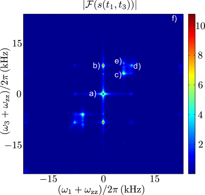
Figure 7: Two-dimensional spectrum obtained for a time evolution given in Eq. (71) where the free evolution is governed by $H_{\rm res}^{(3)}$, Eq. (79). The time evolution includes heating of the modes which leads to broadening of the peaks along the frequency axes. The frequency coordinates of the points a)-f) are given in the text and allow for an identification of all appearing peaks. The complete simulation parameters are given in the main text.

We will now identify the peaks appearing in the spectrum. We start by noting that the peaks in the spectrum can be related by reflections with respect to the origin. Therefore, we will only identify the peaks a)-f) marked in the figure, which is enough to infer the coordinates of all other peaks. In Fig. 8 we illustrate the two pathways leading to the dominant peaks in the spectrum located at a) and b) (and its symmetric counterpart). Both pathways lead to contributions which oscillate at frequency $-\omega_{\rm zz}$ during the free evolution period $t_{1}$. During the second free-evolution period, the contribution from the left pathway also oscillates with $-\omega_{\rm zz}$ while the right pathway has time dependences $-\omega_{\rm zz}\pm\sqrt{2}\Omega_{\rm T}$. The two frequencies in the second time evolution of the right path appear because the state $|n_{\rm zz}=2,n_{\rm str}=0\rangle$ may be written as a superposition of the eigenstates corresponding to the eigenvalues $\pm\sqrt{2}\Omega_{\rm T}$ of $H^{(3)}_{\rm res}$.

Figure 8: Coherence transfer pathways leading to the dominant peaks in the spectrum shown in Fig. 7. The pathway on the left yields a peak at $(-\omega_{\rm zz},-\omega_{\rm zz})$ while the right pathway leads to peaks at $(-\omega_{\rm zz},-\omega_{\rm zz}\pm\sqrt{2}\Omega_{\rm T})$

The peaks identified so far correspond to the possible pathways starting from the motional ground state. In the same way, one can find the pathways which reveal the time dependence during the free evolution periods for contributions where the initial state contains motional excitations, leading to the understanding of the origin of the remaining spectral peaks. The labelled peaks are then found to correspond to the coordinates:

$$\begin{split}{\rm a)}:&(-\omega_{\rm zz},-\omega_{\rm zz}),\\ {\rm b)}:&(-\omega_{\rm zz},-\omega_{\rm zz}+\sqrt{2}\Omega_{\rm T}),\\ {\rm c)}:&(-\omega_{\rm zz}+(\sqrt{6}-\sqrt{2})\Omega_{\rm T},-\omega_{\rm zz}+(\sqrt{6}-\sqrt{2})\Omega_{\rm T}),\\ {\rm d)}:&(-\omega_{\rm zz}+\sqrt{2}\Omega_{\rm T},-\omega_{\rm zz}+\sqrt{2}\Omega_{\rm T}),\\ {\rm e)}:&(-\omega_{\rm zz}+(\sqrt{6}-\sqrt{2})\Omega_{\rm T},\omega_{\rm zz}+(4-\sqrt{6})\Omega_{\rm T}),\\ {\rm f)}:&(-\omega_{\rm zz}+(\sqrt{6}+\sqrt{2})\Omega_{\rm T},-\omega_{\rm zz}+(\sqrt{6}+\sqrt{2})\Omega_{\rm T}).\end{split}$$ (80)

Accordingly, one can identify the eigenvalues of the first three manifolds in Table 5.

References

(1) See R.R. Ernst, G. Bodenhausen and A. Wokaun Principles of Nuclear Magnetic Resonance in One and
Two Dimensions (Oxford University Press, Oxford, 1989) and references therein.
(2)
P. Hamm and M. Zanni, Concepts and Methods of 2D Infrared Spectroscopy
(Cambridge University Press, Cambridge, 2011).
(3)
S. Mukamel, Principles of nonlinear optical spectroscopy (Oxford University Press, Oxford, 1995).
(4)
G. S. Engel et al., Nature 446, 782 (2007).
(5)
S. Ruetzel et al., Proc. Nat. Ac. Sci. 111, 4764 (2014).
(6) D. J. Wineland et al., J. Res. Natl. Inst. Stand. Technol. 103, 259 (1998).
(7)
D. Porras and J. I. Cirac, Phys. Rev. Lett. 92, 207901 (2004).
A. Friedenauer et al., Nat. Phys. 4, 757 (2008).
R. Islam et al., Nature Commun. 2, 377 (2011).
A. Bermudez and M.B. Plenio,
Phys. Rev. Lett. 109, 010501 (2012).
P. A. Ivanov et al., J. Phys. B 46, 104003 (2013).
(8)
A. del Campo et al., Phys. Rev. Lett. 105, 075701 (2010).
S. Ulm et al., Nature Comm. 4, 2290 (2013).
K. Pyka et al., Nature Comm. 4, 2291 (2013).
(9)
A. Bermudez, M. Bruderer and M. B. Plenio, Phys. Rev. Lett. 111, 040601 (2013).
(10)
A. Retzker et al.,
Phys. Rev. Lett. 101, 260504 (2008).
S. Fishman et al., Phys. Rev. B 77, 064111 (2008).
(11)
E. Shimshoni, G. Morigi and S. Fishman, Phys. Rev. Lett. 106, 010401 (2011).
E. Shimshoni, G. Morigi and S. Fishman, Phys. Rev. A 83, 032308 (2011).
(12)
I. Garcia-Mata, O. V. Zhirov and D. L. Shepelyansky, Eur. Phys. J. D 41, 325 (2007).
A. Benassi, A. Vanossi and E. Tosatti, Nature Comm. 2, 236 (2011).
(13)
D. Porras and J. I. Cirac, Phys. Rev. Lett. 93, 263602 (2004).
(14)
M. Gessner et al., New J. Phys. 16, 092001 (2014).
(15) Additional details are provided in section F of the Supplemental Material.
(16)
A. Dantan et al., Phys. Rev. Lett. 105, 103001 (2010).
(17)
B.C. Sawyer et al., Phys. Rev. Lett. 108, 213003 (2012).
(18) Additional details are provided in section D of the Supplemental Material.
(19) C. Marquet, F. Schmidt-Kaler and D. F. V.
James, Appl. Phys. B 76, 199-208 (2003)
(20) Additional details are provided in section C of the Supplemental Material.
(21) Additional details are provided in section A of the Supplemental Material.
(22)
X. R. Nie, C. F. Roos and D. F. V. James, Phys. Lett. A 373, 422-425 (2009).
(23) C. F. Roos et al., Phys. Rev. A 77, 040302(R) (2008)
(24) B. King et al., Phys. Rev. Lett. 81, 1525-1528 (1998)
H. Rohde et al.,
J. Opt. B: Quantum Semiclass. Opt 3, 34-41 (2001)
(25) C. Monroe et al., Science 272, 1131-1135
(1996)
(26) H. Landa, M. Drewsen, B. Reznik, and A. Retzker, New J.
Phys. 14, 093023 (2012).
(27) Additional details are provided in section E of the Supplemental Material.
(28) Additional details are provided in section G of the Supplemental Material.
(29) J. Almeida, J. Prior and M.B. Plenio, J. Phys. Chem. Lett. 3, 2692 - 2696 (2012),
M. Kost, J. Cai, and M. B. Plenio, arXiv:1407.6262

References

(1) D. F. V. James , Appl. Phys. B 66, 181-190 (1998)
(2) C. Marquet, F. Schmidt-Kaler and D. F. V.
James, Appl. Phys. B 76, 199-208 (2003)
(3) H. Goldstein, Klassische Mechanik (Akademische Verlagsgesellschaft, Frankfurt am Main, 1972)
(4)
G. Morigi and S. Fishman, Phys. Rev. Lett. 93, 170602 (2004).
S. Fishman, G. De Chiara, T. Calarco and G. Morigi, Phys. Rev. B 77, 064111 (2008).
(5)
D. G. Enzer et al., Phys. Rev. Lett. 85, 2466 (2000).
(6)
H. Katori, S. Schlipf and H. Walther, Phys. Rev. Lett. 79, 2221 (1997).
(7) C. F. Roos, T. Monz, K. Kim, M. Riebe, H. Häffner, D.F.V. James,
and R. Blatt, et
al., Phys. Rev. A 77, 040302(R) (2008)
(8)
X. R. Nie, C. F. Roos and D. F. V. James, Phys. Lett. A 373, 422-425 (2009).
(9) R.R. Ernst, G. Bodenhausen and A. Wokaun, Principles of Nuclear Magnetic Resonance in One and Two
Dimensions (Oxford University Press, Oxford, 1989)
(10) C. Monroe et al., Science 272, 1131-1135 (1996)
(11)
A. Walther, U. Poschinger, K. Singer and F. Schmidt-Kaler, Appl. Phys. B 107, 1061 – 1067 (2012).
(12)
D. T. Gillespie, Am. J. Phys. 64, 225 (1996).
(13) H.-P. Breuer and F. Petruccione, The Theory of Open Quantum Systems (Oxford University Press, Oxford, 2002)