Phase Retrieval via Wirtinger Flow: Theory and Algorithms
Abstract
We study the problem of recovering the phase from magnitude measurements; specifically, we wish to reconstruct a complex-valued signal about which we have phaseless samples of the form , (knowledge of the phase of these samples would yield a linear system). This paper develops a non-convex formulation of the phase retrieval problem as well as a concrete solution algorithm. In a nutshell, this algorithm starts with a careful initialization obtained by means of a spectral method, and then refines this initial estimate by iteratively applying novel update rules, which have low computational complexity, much like in a gradient descent scheme. The main contribution is that this algorithm is shown to rigorously allow the exact retrieval of phase information from a nearly minimal number of random measurements. Indeed, the sequence of successive iterates provably converges to the solution at a geometric rate so that the proposed scheme is efficient both in terms of computational and data resources. In theory, a variation on this scheme leads to a near-linear time algorithm for a physically realizable model based on coded diffraction patterns. We illustrate the effectiveness of our methods with various experiments on image data. Underlying our analysis are insights for the analysis of non-convex optimization schemes that may have implications for computational problems beyond phase retrieval.
1 Introduction
We are interested in solving quadratic equations of the form
| (1.1) |
where is the decision variable, are known sampling vectors, and are observed measurements. This problem is a general instance of a nonconvex quadratic program (QP). Nonconvex QPs have been observed to occur frequently in science and engineering and, consequently, their study is of importance. For example, a class of combinatorial optimization problems with Boolean decision variables may be cast as QPs [52, Section 4.3.1]. Focusing on the literature on physical sciences, the problem (1.1) is generally referred to as the phase retrieval problem. To understand this connection, recall that most detectors can only record the intensity of the light field and not its phase. Thus, when a small object is illuminated by a quasi-monochromatic wave, detectors measure the magnitude of the diffracted light. In the far field, the diffraction pattern happens to be the Fourier transform of the object of interest—this is called Fraunhofer diffraction—so that in discrete space, (1.1) models the data aquisition mechanism in a coherent diffraction imaging setup; one can identify with the object of interest, with complex sinusoids, and with the recorded data. Hence, we can think of (1.1) as a generalized phase retrieval problem. As is well known, the phase retrieval problem arises in many areas of science and engineering such as X-ray crystallography [33, 48], microscopy [47], astronomy [21], diffraction and array imaging [12, 18], and optics [66]. Other fields of application include acoustics [5, 4], blind channel estimation in wireless communications [3, 58], interferometry [22], quantum mechanics [20, 59] and quantum information [35]. We refer the reader to the tutorial paper [62] for a recent review of the theory and practice of phase retrieval.
Because of the practical significance of the phase retrieval problem in imaging science, the community has developed methods for recovering a signal from data of the form in the special case where one samples the (square) modulus of its Fourier transform. In this setup, the most widely used method is perhaps the error reduction algorithm and its generalizations, which were derived from the pioneering research of Gerchberg and Saxton [29] and Fienup [24, 26]. The Gerchberg-Saxton algorithm starts from a random initial estimate and proceeds by iteratively applying a pair of ‘projections’: at each iteration, the current guess is projected in data space so that the magnitude of its frequency spectrum matches the observations; the signal is then projected in signal space to conform to some a-priori knowledge about its structure. In a typical instance, our knowledge may be that the signal is real-valued, nonnegative and spatially limited. First, while error reduction methods often work well in practice, the algorithms seem to rely heavily on a priori information about the signals, see [34, 60, 25, 27]. Second, since these algorithms can be cast as alternating projections onto nonconvex sets [8] (the constraint in Fourier space is not convex), fundamental mathematical questions concerning their convergence remain, for the most part, unresolved; we refer to Section 3.2 for further discussion.
On the theoretical side, several combinatorial optimization problems—optimization programs with discrete design variables which take on integer or Boolean values—can be cast as solving quadratic equations or as minimizing a linear objective subject to quadratic inequalities. In their most general form these problems are known to be notoriously difficult (NP-hard) [52, Section 4.3]. Nevertheless, many heuristics have been developed for addressing such problems.111For a partial review of some of these heuristics as well as some recent theoretical advances in related problems we refer to our companion paper [16, Section 1.6] and references therein [13, 55, 56, 7, 65, 36, 30, 31]. One popular heuristic is based on a class of convex relaxations known as Shor’s relaxations [52, Section 4.3.1] which can be solved using tractable semi-definite programming (SDP). For certain random models, some recent SDP relaxations such as PhaseLift [14] are known to provide exact solutions (up to global phase) to the generalized phase retrieval problem using a near minimal number of sampling vectors [17, 16]. While in principle SDP based relaxations offer tractable solutions, they become computationally prohibitive as the dimension of the signal increases. Indeed, for a large number of unknowns in the tens of thousands, say, the memory requirements are far out of reach of desktop computers so that these SDP relaxations are de facto impractical.
2 Algorithm: Wirtinger Flow
This paper introduces an approach to phase retrieval based on non-convex optimization as well as a solution algorithm, which has two components: (1) a careful initialization obtained by means of a spectral method, and (2) a series of updates refining this initial estimate by iteratively applying a novel update rule, much like in a gradient descent scheme. We refer to the combination of these two steps, introduced in reverse order below, as the Wirtinger flow (WF) algorithm.
2.1 Minimization of a non-convex objective
Let be a loss function measuring the misfit between both its scalar arguments. If the loss function is non-negative and vanishes only when , then a solution to the generalized phase retrieval problem (1.1) is any solution to
| (2.1) |
Although one could study many loss functions, we shall focus in this paper on the simple quadratic loss . Admittedly, the formulation (2.1) does not make the problem any easier since the function is not convex. Minimizing non-convex objectives, which may have very many stationary points, is known to be NP-hard in general. In fact, even establishing convergence to a local minimum or stationary point can be quite challenging, please see [51] for an example where convergence to a local minimum of a degree-four polynomial is known to be NP-hard.222Observe that if all the sampling vectors are real valued, our objective is also a degree-four polynomial. As a side remark, deciding whether a stationary point of a polynomial of degree four is a local minimizer is already known to be NP-hard.
Our approach to (2.1) is simply stated: start with an initialization , and for , inductively define
| (2.2) |
If the decision variable and the sampling vectors were all real valued, the term between parentheses would be the gradient of divided by two, as our notation suggests. However, since is a mapping from to , it is not holomorphic and hence not complex-differentiable. However, this term can still be viewed as a gradient based on Wirtinger derivatives reviewed in Section 6. Hence, (2.2) is a form of steepest descent and the parameter can be interpreted as a step size (note nonetheless that the effective step size is also inversely proportional to the magnitude of the initial guess).
2.2 Initialization via a spectral method
Our main result states that for a certain random model, if the initialization is sufficiently accurate, then the sequence will converge toward a solution to the generalized phase problem (1.1). In this paper, we propose computing the initial guess via a spectral method, detailed in Algorithm 1. In words, is the leading eigenvector of the positive semidefinite Hermitian matrix constructed from the knowledge of the sampling vectors and observations. (As usual, is the adjoint of .) Letting be the matrix whose th row is so that with obvious notation , is the leading eigenvector of and can be computed via the power method by repeatedly applying , entrywise multiplication by and . In the theoretical framework we study below, a constant number of power iterations would give machine accuracy because of an eigenvalue gap between the top two eigenvalues, please see Appendix B for additional information.
2.3 Wirtinger flow as a stochastic gradient scheme
We would like to motivate the Wirtinger flow algorithm and provide some insight as to why we expect it to work in a model where the sampling vectors are random. First, we emphasize that our statements in this section are heuristic in nature; as it will become clear in the proof Section 7, a correct mathematical formalization of these ideas is far more complicated than our heuristic development here may suggest. Second, although our ideas are broadly applicable, it makes sense to begin understanding the algorithm in a setting where everything is real valued, and in which the vectors are i.i.d. . Also without any loss in generality and to simplify exposition in this section we shall assume .
Let be a solution to (1.1) so that , and consider the initialization step first. In the Gaussian model, a simple moment calculation gives
By the strong law of large numbers, the matrix in Algorithm 1 is equal to the right-hand side in the limit of large samples. Since any leading eigenvector of is of the form for some scalar , we see that the intialization step would recover perfectly, up to a global sign or phase factor, had we infinitely many samples. Indeed, the chosen normalization would guarantee that the recovered signal is of the form . As an aside, we would like to note that the top two eigenvalues of are well separated unless is very small, and that their ratio is equal to . Now with a finite amount of data, the leading eigenvector of will of course not be perfectly correlated with but we hope that it is sufficiently correlated to point us in the right direction.
We now turn our attention to the gradient-update (2.2) and define
where here and below, is once again our planted solution. The first term ensures that the direction of matches the direction of and the second term penalizes the deviation of the Euclidean norm of from that of . Obviously, the minimizers of this function are . Now consider the gradient scheme
| (2.3) |
In Section 7.9, we show that if , then converges to up to a global sign. However, this is all ideal as we would need knowledge of itself to compute the gradient of ; we simply cannot run this algorithm.
Consider now the WF update and assume for a moment that is fixed and independent of the sampling vectors. We are well aware that this is a false assumption but nevertheless wish to explore some of its consequences. In the Gaussian model, if is independent of the sampling vectors, then a modification of Lemma 7.2 for real-valued shows that and, therefore,
Hence, the average WF update is the same as that in (2.3) so that we can interpret the Wirtinger flow algorithm as a stochastic gradient scheme in which we only get to observe an unbiased estimate of the “true” gradient .
Regarding WF as a stochastic gradient scheme helps us in choosing the learning parameter or step size . Lemma 7.7 asserts that
| (2.4) |
holds with high probability. Looking at the right-hand side, this says that the uncertainty about the gradient estimate depends on how far we are from the actual solution . The further away, the larger the uncertainty or the noisier the estimate. This suggests that in the early iterations we should use a small learning parameter as the noise is large since we are not yet close to the solution. However, as the iterations count increases and we make progress, the size of the noise also decreases and we can pick larger values for the learning parameter. This heuristic together with experimentation lead us to consider
| (2.5) |
shown in Figure 1. Values of around and of around worked well in our simulations. This makes sure that is rather small at the beginning (e.g. but quickly increases and reaches a maximum value of about after 200 iterations or so.
3 Main Results
3.1 Exact phase retrieval via Wirtinger flow
Our main result establishes the correctness of the Wirtinger flow algorithm in the Gaussian model defined below. Later in Section 5, we shall also develop exact recovery results for a physically inspired diffraction model.
Definition 3.1
We say that the sampling vectors follow the Gaussian model if . In the real-valued case, they are i.i.d. .
We also need to define the distance to the solution set.
Definition 3.2
Let be any solution to the quadratic system (1.1) (the signal we wish to recover). For each , define
Theorem 3.3
Let be an arbitrary vector in and be quadratic samples with , where is a sufficiently large numerical constant. Then the Wirtinger flow initial estimate normalized to have squared Euclidean norm equal to ,333The same results holds with the intialization from Algorithm 1 because with a standard deviation of about the square root of this quantity. obeys
| (3.1) |
with probability at least ( is a fixed positive numerical constant). Further, take a constant learning parameter sequence, for all and assume for some fixed numerical constant . Then there is an event of probability at least , such that on this event, starting from any initial solution obeying (3.1), we have
Clearly, one would need quadratic measurements to have any hope of recovering . It is also known that in our sampling model, the mapping is injective for [5] and that this property holds for generic sampling vectors [19].444It is not within the scope of this paper to explain the meaning of generic vectors and, instead, refer the interested reader to [19]. Hence, the Wirtinger flow algorithm loses at most a logarithmic factor in the sampling complexity. In comparison, the SDP relaxation only needs a sampling complexity proportional to (no logarithmic factor) [15], and it is an open question whether Theorem 3.3 holds in this regime.
Setting yields accuracy in a relative sense, namely, , in iterations. The computational work at each iteration is dominated by two matrix-vector products of the form and , see Appendix B. It follows that the overall computational complexity of the WF algorithm is . Later in the paper, we will exhibit a modification to the WF algorithm of mere theoretical interest, which also yields exact recovery under the same sampling complexity and an computational complexity; that is to say, the computational workload is now just linear in the problem size.
3.2 Comparison with other non-convex schemes
We now pause to comment on a few other non-convex schemes in the literature. Other comparisons may be found in our companion paper [16].
Earlier, we discussed the Gerchberg-Saxton and Fienup algorithms. These formulations assume that is a Fourier transform and can be described as follows: suppose is the current guess, then one computes the image of through and adjust its modulus so that it matches that of the observed data vector: with obvious notation,
| (3.2) |
where is elementwise multiplication, and so that for all . Then
| (3.3) |
(In the case of Fourier data, the step (3.2)–(3.3) essentially adjusts the modulus of the Fourier transform of the current guess so that it fits the measured data.) Finally, if we know that the solution belongs to a convex set (as in the case where the signal is known to be real-valued, possibly non-negative and of finite support), then the next iterate is
| (3.4) |
where is the projection onto the convex set . If no such information is available, then . The first step (3.3) is not a projection onto a convex set and, therefore, it is in general completely unclear whether the Gerchberg-Saxton algorithm actually converges. (And if it were to converge, at what speed?) It is also unclear how the procedure should be initialized to yield accurate final estimates. This is in contrast to the Wirtinger flow algorithm, which in the Gaussian model is shown to exhibit geometric convergence to the solution to the phase retrieval problem. Another benefit is that the Wirtinger flow algorithm does not require solving a least-squares problem (3.3) at each iteration; each step enjoys a reduced computational complexity.
A recent contribution related to ours is the interesting paper [54], which proposes an alternating minimization scheme named AltMinPhase for the general phase retrieval problem. AltMinPhase is inspired by the Gerchberg-Saxton update (3.2)–(3.3) as well as other established alternating projection heuristics [26, 67, 42, 43, 45, 46]. We describe the algorithm in the setup of Theorem 3.3 for which [54] gives theoretical guarantees. To begin with, AltMinPhase partitions the sampling vectors (the rows of the matrix ) and corresponding observations into disjoint blocks , , , of roughly equal size. Hence, distinct blocks are stochastically independent from each other. The first block is used to compute an initial estimate . After initialization, AltMinPhase goes through a series of iterations of the form (3.2)–(3.3), however, with the key difference that each iteration uses a fresh set of sampling vectors and observations: in details,
| (3.5) |
As for the Gerchberg-Saxton algorithm, each iteration requires solving a least-squares problem. Now assume a real-valued Gaussian model as well as a real valued solution . The main result in [54] states that if the first block contains at least samples and each consecutive block contains at least samples— here denotes a positive numerical constant whose value may change at each occurence—then it is possible to initialize the algorithm via data from the first block in such a way that each consecutive iterate (3.5) decreases the error by 50%; naturally, all of this holds in a probabilistic sense. Hence, one can get accuracy in the sense introduced earlier from a total of samples. Whereas the Wirtinger flow algorithm achieves arbitrary accuracy from just samples, these theoretical results would require an infinite number of samples. This is, however, not the main point.
The main point is that in practice, it is not realistic to imagine (1) that we will divide the samples in distinct blocks (how many blocks should we form a priori? of which sizes?) and (2) that we will use measured data only once. With respect to the latter, observe that the Gerchberg-Saxton procedure (3.2)–(3.3) uses all the samples at each iteration. This is the reason why AltMinPhase is of little practical value, and of theoretical interest only. As a matter of fact, its design and study seem merely to stem from analytical considerations: since one uses an independent set of measurements at each iteration, and are stochastically independent, a fact which considerably simplifies the convergence analysis. In stark contrast, the WF iterate uses all the samples at each iteration and thus introduces some dependencies, which makes for some delicate analysis. Overcoming these difficulties is crucial because the community is preoccupied with convergence properties of algorithms one actually runs, like Gerchberg-Saxton (3.2)–(3.3), or would actually want to run. Interestingly, it may be possible to use some of the ideas developed in this paper to develop a rigorous theory of convergence for algorithms in the style of Gerchberg-Saxton and Fienup, please see [63].
In a recent paper [44], which appeared on the arXiv preprint server as the final version of this paper was under preparation, the authors explore necessary and sufficient conditions for the global convergence of an alternative minimization scheme with generic sampling vectors. The issue is that we do not know when these conditions hold. Further, even when the algorithm converges, it does not come with an explicit convergence rate so that is is not known whether the algorithm converges in polynomial time. As before, some of our methods as well as those from our companion paper [16] may have some bearing upon the analysis of this algorithm. Similarly, another class of nonconvex algorithms that have recently been proposed in the literature are iterative algorithms based on Generalized Approximate Message Passing (GAMP), see [57] and [61] as well as [23, 9, 10] for some background literature on AMP. In [61], the authors demonstrate a favorable runtime for an algorithm of this nature. However, this does not come with any theoretical guarantees.
Moving away from the phase retrieval problem, we would like to mention some very interesting work on the matrix completion problem using non-convex schemes by Montanari and coauthors [39, 40, 38], see also [37, 32, 41, 2, 6, 49, 50]. Although the problems and models are quite different, there are some general similarities between the algorithm named OptSpace in [39] and ours. Indeed, OptSpace operates by computing an initial guess of the solution to a low-rank matrix completion problem by means of a spectral method. It then sets up a nonconvex problem, and proposes an iterative algorithm for solving it. Under suitable assumptions, [39] demonstrates the correctness of this method in the sense that OptSpace will eventually converge to a low-rank solution, although it is not shown to converge in polynomial time.
4 Numerical Experiments
We present some numerical experiments to assess the empirical performance of the Wirtinger flow algorithm. Here, we mostly consider a model of coded diffraction patterns reviewed below.
4.1 The coded diffraction model
We consider an acquisition model, where we collect data of the form
| (4.1) |
thus for a fixed , we collect the magnitude of the diffraction pattern of the signal modulated by the waveform/code . By varying and changing the modulation pattern , we generate several views thereby creating a series of coded diffraction patterns (CDPs).
In this paper, we are mostly interested in the situation where the modulation patterns are random; in particular, we study a model in which the ’s are i.i.d. distributed, each having i.i.d. entries sampled from a distribution . Our theoretical results from Section 5 assume that is symmetric, obeys as well as the moment conditions
| (4.2) |
A random variable obeying these assumptions is said to be admissible. Since is complex valued we can have while . An example of an admissible random variable is , where and are independent and distributed as
| (4.3) |
We shall refer to this distribution as an octanary pattern since can take on eight distinct values. The condition is here to avoid unnecessarily complicated calculations in our theoretical analysis. In particular, we can also work with a ternary pattern in which is distributed as
| (4.4) |
We emphasize that these models are physically realizable in optical applications specially those that arise in microscopy. However, we should note that phase retrieval has many different applications and in some cases other models may be more convenient. We refer to our companion paper [16] Section 2.2 for a discussion of other practically relevant models.
4.2 The Gaussian and coded diffraction models
We begin by examining the performance of the Wirtinger flow algorithm for recovering random signals under the Gaussian and coded diffraction models. We are interested in signals of two different types:
-
•
Random low-pass signals. Here, is given by
with and and are i.i.d. .
-
•
Random Gaussian signals. In this model, is a random complex Gaussian vector with i.i.d. entries of the form with and distributed as ; this can be expressed as
where and are are i.i.d. so that the low-pass model is a ‘bandlimited’ version of this high-pass random model (variances are adjusted so that the expected signal power is the same).
Below, we set , and generate one signal of each type which will be used in all the experiments.
The initialization step of the Wirtinger flow algorithm is run by applying iterations of the power method outlined in Algorithm 3 from Appendix B. In the iteration (2.2), we use the parameter value where . We stop after iterations, and report the empirical probability of success for the two different signal models. The empirical probability of succcess is an average over trials, where in each instance, we generate new random sampling vectors according to the Gaussian or CDP models. We declare a trial successful if the relative error of the reconstruction falls below .
Figure 2 shows that around Gaussian phaseless measurements suffice for exact recovery with high probability via the Wirtinger flow algorithm. We also see that about six octanary patterns are sufficient.
4.3 Performance on natural images
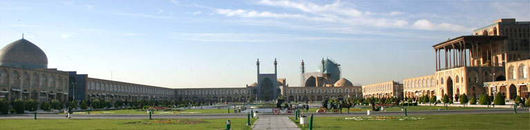
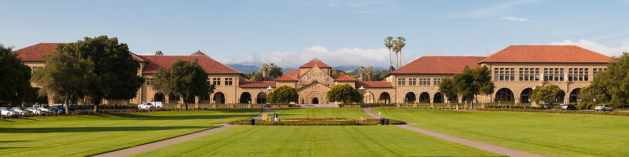
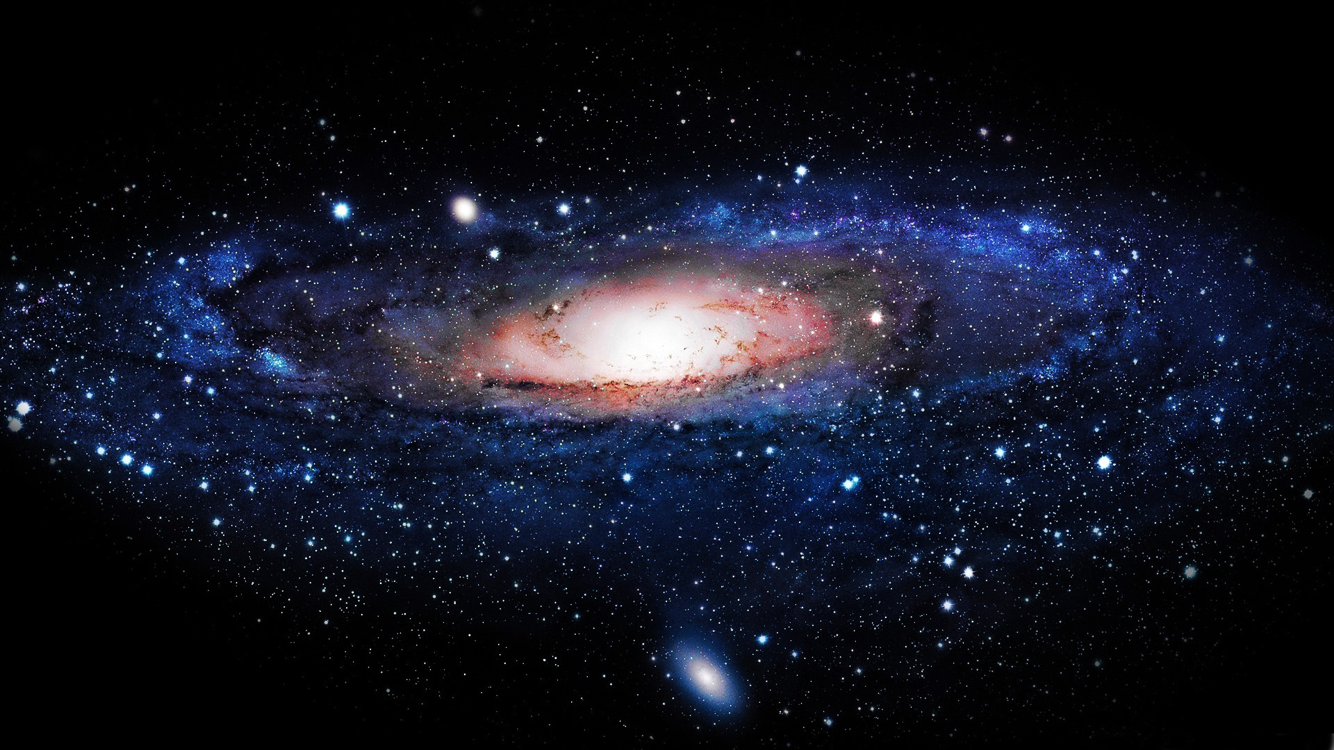
We move on to testing the Wirtinger flow algorithm on various images of different sizes; these are photographs of the Naqsh-e Jahan Square in the central Iranian city of Esfahan, the Stanford main quad, and the Milky Way galaxy. Since each photograph is in color, we run the WF algorithm on each of the three RGB images that make up the photograph. Color images are viewed as arrays, where the first two indices encode the pixel location, and the last the color band.
We generate random octanary patterns and gather the coded diffraction patterns for each color band using these 20 samples. As before, we run 50 iterations of the power method as the initialization step. The updates use the sequence where as before. In all cases we run iterations and record the relative recovery error as well as the running time. If and are the original and recovered images, the relative error is equal to , where is the Euclidean norm . The computational time we report is the the computational time averaged over the three RGB images. All experiments were carried out on a MacBook Pro with a 2.4 GHz Intel Core i7 Processor and 8 GB 1600 MHz DDR3 memory.
Figure 3 shows the images recovered via the Wirtinger flow algorithm. In all cases, WF gets 12 or 13 digits of precision in a matter of minutes. To convey an idea of timing that is platform-independent, we also report time in units of FFTs; one FFT unit is the amount of time it takes to perform a single FFT on an image of the same size. Now all the workload is dominated by matrix vector products of the form and . In details, each iteration of the power method in the initialization step, or each update (2.2) requires FFTs; the factor of 40 comes from the fact that we have 20 patterns and that each iteration involves one FFT and one adjoint or inverse FFT. Hence, the total number of FFTs is equal to
Another way to state this is that the total workload of our algorithm is roughly equal to applications of the sensing matrix and its adjoint . For about 13 digits of accuracy (relative error of about ), Figure 3 shows that we need between 21,000 and 42,000 FFT units. This is within a factor between 1.5 and 3 of the optimal number computed above. This increase has to do with the fact that in our implementation, certain variables are copied into other temporary variables and these types of operations cause some overhead. This overhead is non-linear and becomes more prominent as the size of the signal increases.
For comparison, SDP based solutions such as PhaseLift[17, 14] and PhaseCut[65] would be prohibitive on a laptop computer as the lifted signal would not fit into memory. In the SDP approach an pixel image become an array, which in the first example already takes storing the lifted signal even for the smallest image requires Bytes, which is approximately 85 GB of space. (For the image of the Milky Way, storage would be about 17 TB.) These large memory requirements prevent the application of full-blown SDP solvers on desktop computers.
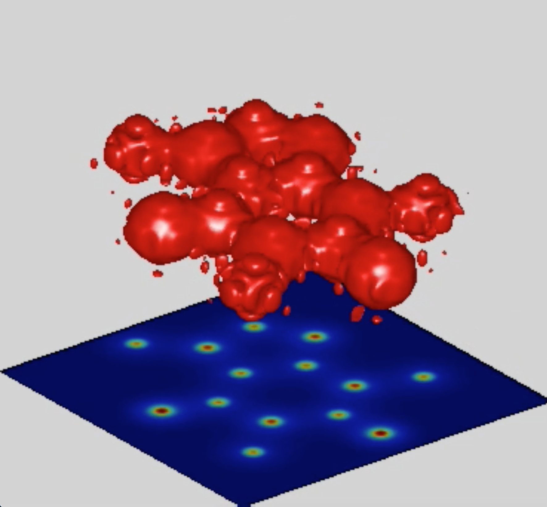
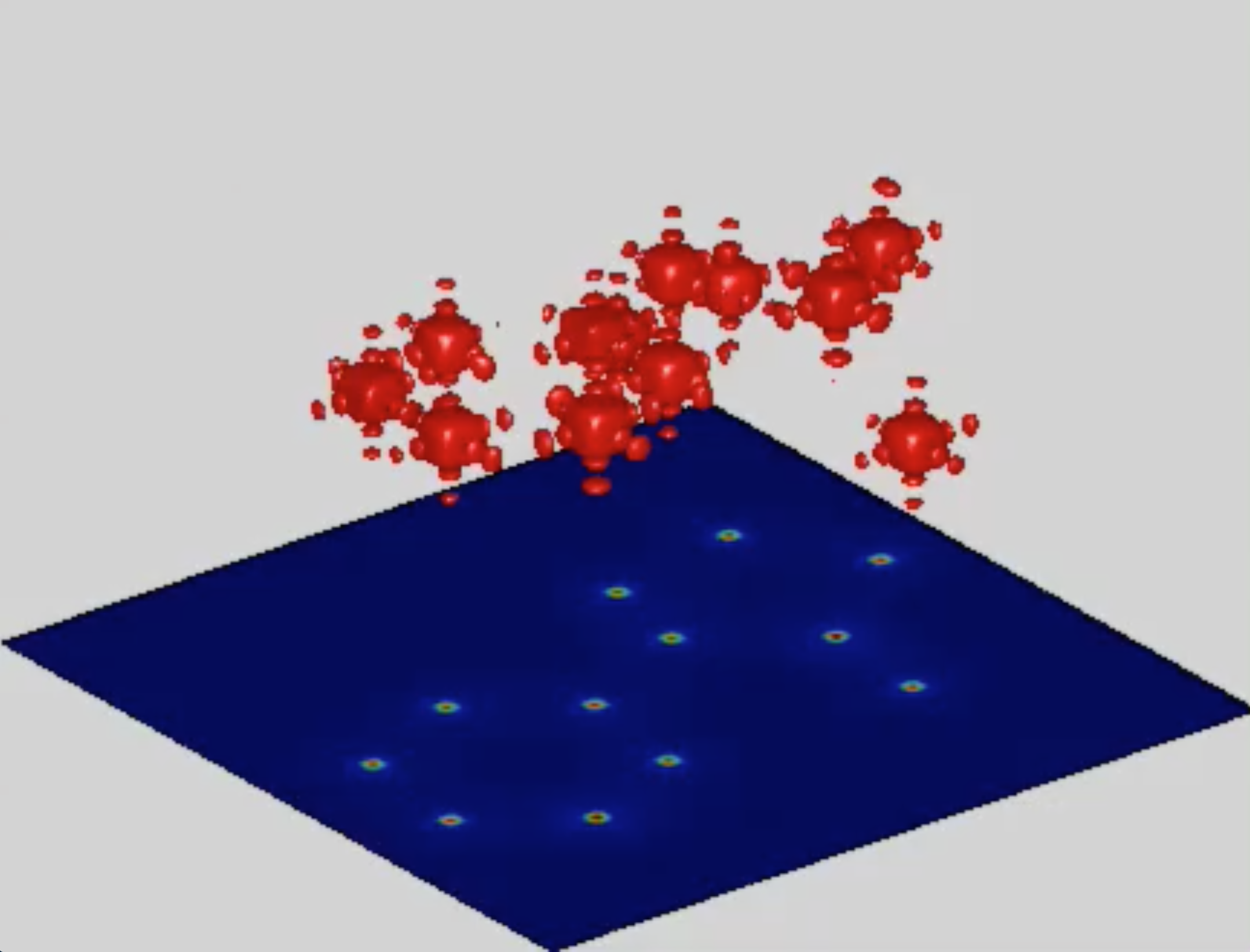
4.4 3D molecules
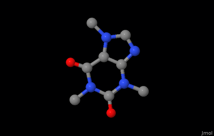
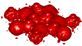
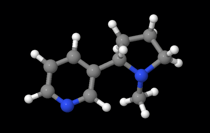
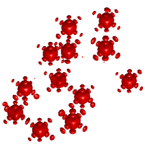
Understanding molecular structure is a great contemporary scientific challenge, and several techniques are currently employed to produce 3D images of molecules; these include electron microscopy and X-ray imaging. In X-ray imaging, for instance, the experimentalist illuminates an object of interest, e.g. a molecule, and then collects the intensity of the diffracted rays, please see Figure 4 for an illustrative setup. Figures 5 and 6 show the schematic representation and the corresponding electron density maps for the Caffeine and Nicotine molecules: the density map is the 3D object we seek to infer. In this paper, we do not go as far 3D reconstruction but demonstrate the performance of the Wirtinger flow algorithm for recovering projections of 3D molecule density maps from simulated data. For related simulations using convex schemes we refer the reader to [28].
To derive signal equations, consider an experimental apparatus as in Figure 4. If we imagine that light propagates in the direction of the -axis, an approximate model for the collected data reads
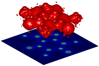
In other words, we collect the intensity of the diffraction pattern of the projection . The 2D image we wish to recover is thus the line integral of the density map along a given direction. As an example, the Caffeine molecule along with its projection on the -plane (line integral in the direction) is shown in Figure 7. Now, if we let be the Fourier transform of the density , one can re-express the identity above as
Therefore, by imputing the missing phase using phase retrieval algorithms, one can recover a slice of the 3D Fourier transfom of the electron density map, i.e. . Viewing the object from different angles or directions gives us different slices. In a second step we do not perform in this paper, one can presumably recover the 3D Fourier transform of the electron density map from all these slices (this is the tomography or blind tomography problem depending upon whether or not the projection angles are known) and, in turn, the 3D electron density map.
We now generate observation planes by rotating the -plane around the -axis by equally spaced angles in the interval . Each of these planes is associated with a 2D projection of size , giving us 20 coded diffraction octanary patterns (we use the same patterns for all 51 projections). We run the Wirtinger flow algorithm with exactly the same parameters as in the previous section, and stop after 150 gradient iterations. Figure 8 reports the average relative error over the 51 projections and the total computational time required for reconstructing all 51 images.
Mean rel. error is
Total time is hours
Mean rel. error is
Total time is hours
5 Theory for the Coded Diffraction Model
We complement our study with theoretical results applying to the model of coded diffraction patterns. These results concern a variation of the Wirtinger flow algorithm: whereas the iterations are exactly the same as (2.2), the initialization applies an iterative scheme which uses fresh sets of sample at each iteration. This is described in Algorithm 2. In the CDP model, the partitioning assigns to the same group all the observations and sampling vectors corresponding to a given realization of the random code. This is equivalent to partitioning the random patterns into groups. As a result, sampling vectors in distinct groups are stochastically independent.
Theorem 5.1
Let be an arbitrary vector in and assume we collect admissible coded diffraction patterns with , where is a sufficiently large numerical constant. Then the initial solution of Algorithm 2555We choose the number of partitions in Algorithm 2 to obey for a sufficiently large numerical constant. obeys
| (5.1) |
with probability at least . Further, take a constant learning parameter sequence, for all and assume for some fixed numerical constant . Then there is an event of probability at least , such that on this event, starting from any initial solution obeying (5.1), we have
| (5.2) |
In the Gaussian model, both statements also hold with high probability provided that , where is a sufficiently large numerical constant.
Hence, we achieve perfect recovery from on the order of samples arising from a coded diffraction experiment. Our companion paper [16] established that PhaseLift—the SDP relaxation—is also exact with a sampling complexity on the order of (this has recently been improved to [31]). We believe that the sampling complexity of both approaches (WF and SDP) can be further reduced to (or even for certain kind of patterns). We leave this to future research.
Setting yields accuracy in iterations. As the computational work at each iteration is dominated by two matrix-vector products of the form and , it follows that the overall computational is at most . In particular, this approach yields a near-linear time algorithm in the CDP model (linear in the dimension of the signal ). In the Gaussian model, the complexity scales like .
6 Wirtinger Derivatives
Our gradient step (2.2) uses a notion of derivative, which can be interpreted as a Wirtinger derivative. The purpose of this section is thus to gather some results concerning Wirtinger derivatives of real valued functions over complex variables. Here and below, is the transpose of the matrix , and denotes the complex conjugate of a scalar . Similarly, the matrix is obtained by taking complex conjugates of the elements of .
Any complex-or real-valued function
of several complex variables can be written in the form , where is holomorphic in for fixed and holomorphic in for fixed . This holds as long as a the real-valued functions and are differentiable as functions of the real variables and . As an example, consider
with and . While is not holomorphic in , is holomorphic in for a fixed , and vice versa.
This fact underlies the development of the Wirtinger calculus. In essence, the conjugate coordinates
can serve as a formal substitute for the representation . This leads to the following derivatives
Our definitions follow standard notation from multivariate calculus so that derivatives are row vectors and gradients are column vectors. In this new coordinate system the complex gradient is given by
Similarly, we define
In this coordinate system the complex Hessian is given by
Given vectors and , we have defined the gradient and Hessian in a manner such that Taylor’s approximation takes the form
If we were to run gradient descent in this new coordinate system, the iterates would be
| (6.1) |
Note that when is a real-valued function (as in this paper) we have
Therefore, the second set of updates in (6.1) is just the conjugate of the first. Thus, it is sufficient to keep track of the first update, namely,
For real valued functions of complex variables, setting
gives the gradient update
The reader may wonder why we choose to work with conjugate coordinates as there are alternatives: in particular, we could view the complex variable as a vector in and just run gradient descent in the coordinate system. The main reason why conjugate coordinates are particularly attractive is that expressions for derivatives become significantly simpler and resemble those we obtain in the real case, where is a function of real variables.
7 Proofs
7.1 Preliminaries
We first note that in the CDP model with admissible CDPs for all , as in our CDP model . In the Gaussian model the measurements vectors also obey for all with probability at least . Throughout the proofs, we assume we are on this event without explicitly mentioning it each time.
Before we begin with the proofs we should mention that we will prove our result using the update
| (7.1) |
in lieu of the WF update
| (7.2) |
Since holds with high probability as proven in Section 7.8, we have
| (7.3) |
Therefore, the results for the update (7.1) automatically carry over to the WF update with a simple rescaling of the upper bound on the learning parameter. More precisely, if we prove that the update (7.1) converges to a global optimum as long as , then the convergence of the WF update to a global optimum is guaranteed as long as . Also, the update in (7.1) is invariant to the Euclidean norm of . Therefore, without loss of generality we will assume throughout the proofs that .
We remind the reader that throughout is a solution to our quadratic equations, i.e. obeys and that the sampling vectors are independent from . Define
to be the set of all vectors that differ from the planted solution only by a global phase factor. We also introduce the set of all points that are close to ,
| (7.4) |
Finally for any vector we define the phase as
so that
7.2 Formulas for the complex gradient and Hessian
We gather some useful gradient and Hessian calculations that will be used repeatedly. Starting with
we establish
This gives
For the second derivative, we write
and
Therefore,
7.3 Expectation and concentration
This section gathers some useful intermediate results whose proofs are deferred to Appendix A. The first two lemmas establish the expectation of the Hessian, gradient and a related random variable in both the Gaussian and admissible CDP models.666In the CDP model the expectation is with respect to the random modulation pattern.
Lemma 7.1
Recall that is a solution obeying , which is independent from the sampling vectors. Furthermore, assume the sampling vectors are distributed according to either the Gaussian or admissible CDP model. Then
Lemma 7.2
In the setup of Lemma 7.1, let be a fixed vector independent of the sampling vectors. We have
The next lemma gathers some useful identities in the Gaussian model.
Lemma 7.3
Assume are fixed vectors obeying which are independent of the sampling vectors. Furthermore, assume the measurement vectors are distributed according to the Gaussian model. Then
| (7.5) | ||||
| (7.6) | ||||
| (7.7) |
The next lemma establishes the concentration of the Hessian around its mean for both the Gaussian and the CDP model.
Lemma 7.4
In the setup of Lemma 7.1, assume the vectors are distributed according to either the Gaussian or admissible CDP model with a sufficiently large number of measurements. This means that the number of samples obeys in the Gaussian model and the number of patterns obeys in the CDP model. Then
| (7.8) |
holds with probability at least and for the Gaussian and CDP models, respectively.
We will also make use of the two results below, which are corollaries of the three lemmas above. These corollaries are also proven in Appendix A.
Corollary 7.5
Suppose . Then for all obeying , we have
In the other direction,
Corollary 7.6
Suppose . Then for all obeying , we have
and
The next lemma establishes the concentration of the gradient around its mean for both Gaussian and admissible CDP models.
Lemma 7.7
In the setup of Lemma 7.4, let be a fixed vector independent of the sampling vectors obeying . Then
holds with probability at least in the Gaussian model and in the CDP model.
We finish with a result concerning the concentration of the sample covariance matrix.
Lemma 7.8
In the setup of Lemma 7.4,
holds with probability at least for the Gaussian model and in the CDP model. On this event,
| (7.9) |
7.4 General convergence analysis
We will assume that the function satisfies a regularity condition on , which essentially states that the gradient of the function is well behaved. We remind the reader that , as defined in (7.4), is the set of points that are close to the path of global minimizers.
Condition 7.9 (Regularity Condition)
We say that the function satisfies the regularity condition or if for all vectors we have
| (7.10) |
In the lemma below we show that as long as the regularity condition holds on then Wirtinger Flow starting from an initial solution in converges to a global optimizer at a geometric rate. Subsequent sections shall establish that this property holds.
Lemma 7.10
Assume that obeys RC for all . Furthermore, suppose , and assume . Consider the following update
Then for all we have and
We note that for , (7.10) holds with the direction of the inequality reversed.777One can see this by applying Cauchy-Schwarz and calculating the determinant of the resulting quadratic form. Thus, if holds, and must obey . As a result, under the stated assumptions of Lemma 7.10 above, the factor is non-negative.
Proof The proof follows a structure similar to related results in the convex optimization literature e.g. [53, Theorem 2.1.15]. However, unlike these classical results where the goal is often to prove convergence to a unique global optimum, the objective function does not have a unique global optimum. Indeed, in our problem, if is solution, then is also solution. Hence, proper modification is required to prove convergence results.
7.5 Proof of the regularity condition
For any , we need to show that
| (7.12) |
We prove this with by establishing that our gradient satisfies the local smoothness and local curvature conditions defined below. Combining both these two properties gives (7.12).
Condition 7.11 (Local Curvature Condition)
We say that the function satisfies the local curvature condition or if for all vectors ,
| (7.13) |
This condition essentially states that the function curves sufficiently upwards (along most directions) near the curve of global optimizers.
Condition 7.12 (Local Smoothness Condition)
We say that the function satisfies the local smoothness condition or if for all vectors we have
| (7.14) |
This condition essentially states that the gradient of the function is well behaved (the function does not vary too much) near the curve of global optimizers.
7.6 Proof of the local curvature condition
For any , we want to prove the local curvature condition (7.13). Recall that
and define . To establish (7.13) it suffices to prove that
| (7.15) |
holds for all satisfying , . Equivalently, we only need to prove that for all satisfying , and for all with ,
| (7.16) |
By Corollary 7.5, with high probability,
holds for all obeying . Therefore, to establish the local curvature condition (7.13) it suffices to show that
| (7.17) |
We will establish (7.17) for different measurement models and different values of . Below, it shall be convenient to use the shorthand
7.6.1 Proof of (7.17) with in the Gaussian and CDP models
Set . We show that with high probability, (7.17) holds for all satisfying Im, , , , and . First, note that by Cauchy-Schwarz inequality,
| (7.18) |
The last inequality follows from . By Corollary 7.5,
| (7.19) |
holds with high probability for all obeying . Furthermore, by applying Lemma 7.8,
| (7.20) |
holds with high probability. Plugging (7.19) and (7.20) in (7.6.1) yields
(7.17) follows by using , and .
7.6.2 Proof of (7.17) with in the Gaussian model
Set . We show that with high probability, (7.17) holds for all satisfying , , , , and . To this end, we first state a result about the tail of a sum of i.i.d. random variables. Below, is the cumulative distribution function of a standard normal variable.
Lemma 7.13 ([11])
Suppose are i.i.d. real-valued random variables obeying for some nonrandom , , and . Setting ,
where one can take .
To establish (7.17) we first prove it for a fixed , and then use a covering argument. Observe that
By Lemma 7.3,
compare (7.5) and (7.6). Therefore, using ,
Now define . First, since , . Second, we bound using Lemma 7.3 and Holder’s inequality with :
We have all the elements to apply Lemma 7.13 with and :
with . Therefore, with probability at least , we have
| (7.21) |
provided that . The inequality above holds for a fixed vector and a fixed value . To prove (7.17) for all and all with , define
Using the fact that and , we have . Moreover, for any obeying ,
Introduce
For any obeying ,
| (7.22) |
Therefore, for any obeying and , we have
| (7.23) |
Let be an -net for the unit sphere of with cardinality obeying . Applying (7.6.2) together with the union bound we conclude that for all and a fixed
| (7.24) |
The last line follows by choosing such that , where is a sufficiently large constant. Now for any on the unit sphere of , there exists a vector such that . By combining (7.23) and (7.6.2), holds with probability at least for all with unit Euclidean norm and for a fixed . Applying a similar covering number argument over we can further conclude that for all and
holds with probability at least as long as . This concludes the proof of (7.17) with .
7.7 Proof of the local smoothness condition
For any , we want to prove (7.14), which is equivalent to proving that for all obeying , we have
Recall that
and define
Define and , to establish (7.14) it suffices to prove that
| (7.25) |
holds for all and satisfying Im, and . Equivalently, we only need to prove for all and satisfying Im, and ,
| (7.26) |
Note that since
| (7.27) |
We now bound each of the terms on the right-hand side. For the first term we use Cauchy-Schwarz and Corollary 7.6, which give
| (7.28) |
Similarly, for the second term, we have
| (7.29) |
Finally, for the third term we use the Cauchy-Schwarz inequality together with Lemma 7.8 (inequality) (7.9) to derive
| (7.30) |
We now plug these inequalities into (7.7) and get
| (7.31) |
which completes the proof of (7.26) and, in turn, establishes the local smoothness condition in (7.14). However, the last line of (7.7) holds as long as
| (7.32) |
In our theorems we use two different values of and . Using in (7.32) we conclude that the local smoothness condition (7.7) holds as long as
7.8 Wirtinger flow initialization
In this section, we prove that the WF initialization obeys (3.1) from Theorem 3.3. Recall that
and that Lemma 7.4 gives
Let be the eigenvector corresponding to the top eigenvalue of obeying . It is easy to see that
Therefore,
Also, since is the top eigenvalue of , and , we have
Combining the above two inequalities together, we have
Recall that . By Lemma 7.8, equation (7.9), with high probability we have
Therefore, we have
7.9 Initialization via resampled Wirtinger Flow
In this section, we prove that that the output of Algorithm 2 obeys (5.1) from Theorem 5.1. Introduce
By Lemma 7.2, if is a vector independent from the measurements, then
We prove that obeys a regularization condition in , namely,
| (7.33) |
Lemma 7.7 implies that for a fixed vector ,
| (7.34) |
holds with high probability. The last inequality follows from (7.33). Applying Lemma 7.7, we also have
Plugging the latter into (7.9) yields
Therefore, using the general convergence analysis of gradient descent discussed in Section 7.4 we conclude that for all ,
Finally,
It only remains to establish (7.33). First, without loss of generality, we can assume that , which implies and use in lieu of dist. Set so that . This implies
Therefore,
| (7.35) |
where the last inequality is due to . Furthermore,
| (7.36) |
where the last inequality also holds because . Finally, (7.35) and (7.9) imply
where and .
Acknowledgements
E. C. is partially supported by AFOSR under grant FA9550-09-1-0643 and by gift from the Broadcom Foundation. X. L. is supported by the Wharton Dean’s Fund for Post-Doctoral Research and by funding from the National Institutes of Health. M. S. is supported by a Benchmark Stanford Graduate Fellowship and AFOSR grant FA9550-09-1-0643. M. S. would like to thank Andrea Montanari for helpful discussions and for the class [1] which inspired him to explore provable algorithms based on non-convex schemes. He would also like to thank Alexandre d’Aspremont, Fajwel Fogel and Filipe Maia for sharing some useful code regarding 3D molecule reconstructions, Ben Recht for introducing him to reference [51], and Amit Singer for bringing the paper [44] to his attention.
References
- [1] Stanford EE 378B: Inference, Estimation, and Information Processing.
- [2] A. Agarwal, S. Negahban, and M. J. Wainwright. Fast global convergence of gradient methods for high-dimensional statistical recovery. The Annals of Statistics, 40(5):2452–2482, 2012.
- [3] A. Ahmed, B. Recht, and J. Romberg. Blind deconvolution using convex programming. arXiv preprint arXiv:1211.5608, 2012.
- [4] R. Balan. On signal reconstruction from its spectrogram. In Information Sciences and Systems (CISS), 2010 44th Annual Conference on, pages 1–4. IEEE, 2010.
- [5] R. Balan, P. Casazza, and D. Edidin. On signal reconstruction without phase. Applied and Computational Harmonic Analysis, 20(3):345–356, 2006.
- [6] L. Balzano and S. J. Wright. Local convergence of an algorithm for subspace identification from partial data. arXiv preprint arXiv:1306.3391, 2013.
- [7] A. S. Bandeira, J. Cahill, D. G. Mixon, and A. A. Nelson. Saving phase: Injectivity and stability for phase retrieval. arXiv preprint arXiv:1302.4618, 2013.
- [8] H. H. Bauschke, P. L. Combettes, and D. R. Luke. Hybrid projection–reflection method for phase retrieval. JOSA A, 20(6):1025–1034, 2003.
- [9] M. Bayati and A. Montanari. The dynamics of message passing on dense graphs, with applications to compressed sensing. Information Theory, IEEE Transactions on, 57(2):764–785, 2011.
- [10] M. Bayati and A. Montanari. The LASSO risk for Gaussian matrices. Information Theory, IEEE Transactions on, 58(4):1997–2017, 2012.
- [11] V. Bentkus. An inequality for tail probabilities of martingales with differences bounded from one side. Journal of Theoretical Probability, 16(1):161–173, 2003.
- [12] O. Bunk, A. Diaz, F. Pfeiffer, C. David, B. Schmitt, D. K. Satapathy, and J. F Veen. Diffractive imaging for periodic samples: retrieving one-dimensional concentration profiles across microfluidic channels. Acta Crystallographica Section A: Foundations of Crystallography, 63(4):306–314, 2007.
- [13] J. Cahill, P. G. Casazza, J. Peterson, and L. Woodland. Phase retrieval by projections.
- [14] E. J. Candes, Y. C Eldar, T. Strohmer, and V. Voroninski. Phase retrieval via matrix completion. SIAM Journal on Imaging Sciences, 6(1):199–225, 2013.
- [15] E. J. Candes and X. Li. Solving quadratic equations via phaselift when there are about as many equations as unknowns. Foundations of Computational Mathematics, pages 1–10, 2012.
- [16] E. J. Candès, X. Li, and M. Soltanolkotabi. Phase retrieval from coded diffraction patterns. arXiv:1310.3240, Preprint 2013.
- [17] E. J. Candes, T. Strohmer, and V. Voroninski. Phaselift: Exact and stable signal recovery from magnitude measurements via convex programming. Communications on Pure and Applied Mathematics, 2012.
- [18] A. Chai, M. Moscoso, and G. Papanicolaou. Array imaging using intensity-only measurements. Inverse Problems, 27(1):015005, 2011.
- [19] A. Conca, D. Edidin, M. Hering, and C. Vinzant. An algebraic characterization of injectivity in phase retrieval. arXiv preprint arXiv:1312.0158, 2013.
- [20] J. V. Corbett. The Pauli problem, state reconstruction and quantum-real numbers. Reports on Mathematical Physics, 57(1):53–68, 2006.
- [21] J. C. Dainty and J. R. Fienup. Phase retrieval and image reconstruction for astronomy. Image Recovery: Theory and Application, ed. by H. Stark, Academic Press, San Diego, pages 231–275, 1987.
- [22] L. Demanet and V. Jugnon. Convex recovery from interferometric measurements. arXiv preprint arXiv:1307.6864, 2013.
- [23] D. L. Donoho, A. Maleki, and A. Montanari. Message-passing algorithms for compressed sensing. Proceedings of the National Academy of Sciences, 106(45):18914–18919, 2009.
- [24] J. R. Fienup. Reconstruction of an object from the modulus of its Fourier transform. Optics letters, 3(1):27–29, 1978.
- [25] J. R. Fienup. Fine resolution imaging of space objects. Final Scientific Report, 1 Oct. 1979-31 Oct. 1981 Environmental Research Inst. of Michigan, Ann Arbor. Radar and Optics Div., 1, 1982.
- [26] J. R. Fienup. Phase retrieval algorithms: a comparison. Applied optics, 21(15):2758–2769, 1982.
- [27] J. R. Fienup. Comments on “The reconstruction of a multidimensional sequence from the phase or magnitude of its Fourier transform”. Acoustics, Speech and Signal Processing, IEEE Transactions on, 31(3):738–739, 1983.
- [28] F. Fogel, I. Waldspurger, and A. d’Aspremont. Phase retrieval for imaging problems. arXiv preprint arXiv:1304.7735, 2013.
- [29] R. W. Gerchberg. A practical algorithm for the determination of phase from image and diffraction plane pictures. Optik, 35:237, 1972.
- [30] D. Gross, F. Krahmer, and R. Kueng. A partial derandomization of phaselift using spherical designs. arXiv preprint arXiv:1310.2267, 2013.
- [31] D. Gross, F. Krahmer, and R. Kueng. Improved recovery guarantees for phase retrieval from coded diffraction patterns. arXiv preprint arXiv:1402.6286, 2014.
- [32] M. Hardt. On the provable convergence of alternating minimization for matrix completion. arXiv preprint arXiv:1312.0925, 2013.
- [33] R. W. Harrison. Phase problem in crystallography. JOSA A, 10(5):1046–1055, 1993.
- [34] M. H. Hayes. The reconstruction of a multidimensional sequence from the phase or magnitude of its Fourier transform. Acoustics, Speech and Signal Processing, IEEE Transactions on, 30(2):140–154, 1982.
- [35] T. Heinosaari, L. Mazzarella, and M. M. Wolf. Quantum tomography under prior information. Communications in Mathematical Physics, 318(2):355–374, 2013.
- [36] K. Jaganathan, S. Oymak, and B. Hassibi. On robust phase retrieval for sparse signals. In Communication, Control, and Computing (Allerton), 2012 50th Annual Allerton Conference on, pages 794–799. IEEE, 2012.
- [37] P. Jain, P. Netrapalli, and S. Sanghavi. Low-rank matrix completion using alternating minimization. In Proceedings of the 45th annual ACM symposium on Symposium on theory of computing, pages 665–674. ACM, 2013.
- [38] R. H. Keshavan. Efficient algorithms for collaborative filtering. PhD thesis, Stanford University, 2012.
- [39] R. H. Keshavan, A. Montanari, and S. Oh. Matrix completion from a few entries. Information Theory, IEEE Transactions on, 56(6):2980–2998, 2010.
- [40] R. H. Keshavan, A. Montanari, and S. Oh. Matrix completion from noisy entries. The Journal of Machine Learning Research, 99:2057–2078, 2010.
- [41] K. Lee, Y. Wu, and Y. Bresler. Near optimal compressed sensing of sparse rank-one matrices via sparse power factorization. arXiv preprint arXiv:1312.0525, 2013.
- [42] S. Marchesini. Invited article: A unified evaluation of iterative projection algorithms for phase retrieval. Review of Scientific Instruments, 78(1):011301, 2007.
- [43] S. Marchesini. Phase retrieval and saddle-point optimization. JOSA A, 24(10):3289–3296, 2007.
- [44] S. Marchesini, Y. C. Tu, and H. Wu. Alternating projection, ptychographic imaging and phase synchronization. arXiv preprint arXiv:1402.0550, 2014.
- [45] J. Miao, P. Charalambous, J. Kirz, and D. Sayre. Extending the methodology of x-ray crystallography to allow imaging of micrometre-sized non-crystalline specimens. Nature, 400(6742):342–344, 1999.
- [46] J. Miao, T. Ishikawa, B. Johnson, E. H. Anderson, B. Lai, and K. O. Hodgson. High resolution 3D x-ray diffraction microscopy. Physical review letters, 89(8):088303, 2002.
- [47] J. Miao, T. Ishikawa, Q. Shen, and T. Earnest. Extending x-ray crystallography to allow the imaging of noncrystalline materials, cells, and single protein complexes. Annu. Rev. Phys. Chem., 59:387–410, 2008.
- [48] R. P. Millane. Phase retrieval in crystallography and optics. JOSA A, 7(3):394–411, 1990.
- [49] Y. Mroueh. Robust phase retrieval and super-resolution from one bit coded diffraction patterns. arXiv preprint arXiv:1402.2255, 2014.
- [50] Y. Mroueh and L. Rosasco. Quantization and greed are good: One bit phase retrieval, robustness and greedy refinements. arXiv preprint arXiv:1312.1830, 2013.
- [51] K. G. Murty and S. N. Kabadi. Some NP-complete problems in quadratic and nonlinear programming. Mathematical programming, 39(2):117–129, 1987.
- [52] A. Nemirovski. Lectures on modern convex optimization. In Society for Industrial and Applied Mathematics (SIAM). Citeseer, 2001.
- [53] Y. Nesterov. Introductory lectures on convex optimization, volume 87 of Applied Optimization. Kluwer Academic Publishers, Boston, MA, 2004. A basic course.
- [54] P. Netrapalli, P. Jain, and S. Sanghavi. Phase retrieval using alternating minimization. arXiv preprint arXiv:1306.0160, 2013.
- [55] H. Ohlsson, A. Y. Yang, R. Dong, and S. S. Sastry. Compressive phase retrieval from squared output measurements via semidefinite programming. arXiv preprint arXiv:1111.6323, 2011.
- [56] S. Oymak, A. Jalali, M. Fazel, Y. C. Eldar, and B. Hassibi. Simultaneously structured models with application to sparse and low-rank matrices. arXiv preprint arXiv:1212.3753, 2012.
- [57] S. Rangan. Generalized approximate message passing for estimation with random linear mixing. In Information Theory Proceedings (ISIT), 2011 IEEE International Symposium on, pages 2168–2172. IEEE, 2011.
- [58] J. Ranieri, A. Chebira, Y. M. Lu, and M. Vetterli. Phase retrieval for sparse signals: Uniqueness conditions. arXiv preprint arXiv:1308.3058, 2013.
- [59] H. Reichenbach. Philosophic foundations of quantum mechanics. University of California Pr, 1965.
- [60] J. L. C. Sanz, T. S. Huang, and T. Wu. A note on iterative Fourier transform phase reconstruction from magnitude. Acoustics, Speech and Signal Processing, IEEE Transactions on, 32(6):1251–1254, 1984.
- [61] P. Schniter and S. Rangan. Compressive phase retrieval via generalized approximate message passing. In Communication, Control, and Computing (Allerton), 2012 50th Annual Allerton Conference on, pages 815–822. IEEE, 2012.
- [62] Y. Shechtman, Y. C. Eldar, O. Cohen, H. N. Chapman, J. Miao, and M. Segev. Phase retrieval with application to optical imaging. arXiv preprint arXiv:1402.7350, 2014.
- [63] M. Soltanolkotabi. Algorithms and Theory for Clustering and Nonconvex Quadratic Programming. Stanford Ph.D. Dissertation, 2014.
- [64] R. Vershynin. Introduction to the non-asymptotic analysis of random matrices, 2011. Cambridge University Press, Y. C. Eldar and G. Kutyniok, editors, Compressed Sensing: Theory and Applications, 2012.
- [65] I. Waldspurger, A. d’Aspremont, and S. Mallat. Phase recovery, maxcut and complex semidefinite programming. arXiv preprint arXiv:1206.0102, 2012.
- [66] A. Walther. The question of phase retrieval in optics. Journal of Modern Optics, 10(1):41–49, 1963.
- [67] G. Yang, B. Dong, B. Gu, J. Zhuang, and O. K. Ersoy. Gerchberg-Saxton and Yang-Gu algorithms for phase retrieval in a nonunitary transform system: a comparison. Applied optics, 33(2):209–218, 1994.
Appendix A Expectations and deviations
We provide here the proofs of our intermediate results. Throughout this section we use to denote a diagonal random matrix with diagonal elements being i.i.d. samples from an admissible distribution (recall the definition (4.2) of an admissible random variable). For ease of exposition, we shall rewrite (4.1) in the form
where is the th row of the DFT matrix and is a diagonal matrix with the diagonal entries given by . In our model, the matricces are i.i.d. copies of .
A.1 Proof of Lemma 7.1
The proof for admissible coded diffraction patterns follows from Lemmas 3.1 and 3.2 in [16]. For the Gaussian model, it is a consequence of the two lemmas below, whose proofs are ommitted.
Lemma A.1
Suppose the sequence follows the Gaussiam model. Then for any fixed vector ,
Lemma A.2
Suppose the sequence follows the Gaussiam model. Then for any fixed vector ,
A.2 Proof of Lemma 7.2
A.3 Proof of Lemma 7.3
Suppose . Since the law of is invariant by unitary transformation, we may just as well take and , where are positive real numbers obeying . We have
and
The identity (7.7) follows from standard normal moment calculations.
A.4 Proof of Lemma 7.4
A.4.1 The CDP model
Write the Hessian as
where
and
It is useful to recall that
Now set
where is a positive scalar whose value will be determined shortly, and define the events
Note that . Also, if for all pairs , then and thus . Putting all of this together gives
| (A.1) |
A slight modification to Lemma 3.9 in [16] gives provided for a sufficiently large numerical constant . Since Hoeffding’s inequality yields , we have
Setting completes the proof.
A.4.2 The Gaussian model
By unitary invariance, we may take . Letting , be the first coordinate of a vector , to prove Lemma 7.4 for the Gaussian model it suffices to prove the two inequalities,
| (A.2) |
and
| (A.3) |
For any , there is a constant with the property that implies
with probability at least ; this is a consquence of Chebyshev’s inequality. Moreover a union bound gives
with probability at least . Denote by the event on which the above inequalities hold. We show that there is another event of high probability such that (A.2) and (A.3) hold on . Our proof strategy is similar to that of Theorem 39 in [64]. To prove (A.2), we will show that with high probability, for any obeying , we have
| (A.4) |
For this purpose, partition in the form with , and decompose the inner product as
This gives
which follows from since has unit norm. This gives
| (A.5) |
We now turn our attention to the last two terms of (A.4.2). For the second term, the ordinary Hoeffding’s inequality (Proposition 10 in [64]) gives that for any constants and , there exists a constant , such that for ,
holds with probability at least . To control the final term, we apply the Bernstein-type inequality (Proposition 16 in [64]) to assert the following: for any positive constants and , there exists a constant , such that for ,
holds with probability at least .
Therefore, for any unit norm vector ,
| (A.6) |
holds with probability at least . By Lemma 5.4 in [64], we can bound the operator norm via an -net argument:
where is an -net of the unit sphere in . By applying the union bound and choosing appropriate , and , (A.2) holds with probability at least , as long as . On this inequality follows from provided is sufficiently large. In conclusion, (A.2) holds with probability at least .
The proof of (A.3) is similar. The only difference is that the random matrix is not Hermitian, so we work with
where and are unit vectors.
A.5 Proof of Corollary 7.5
It follows from that . Therefore, using the fact that for any complex scalar , , we have
The other inequality is established in a similar fashion.
A.6 Proof of Corollary 7.6
In the proof of Lemma 7.4, we established that with high probability,
Therefore,
This concludes the proof of one side. The other side is similar.
A.7 Proof of Lemma 7.7
A.8 Proof of Lemma 7.8
Appendix B The Power Method
We use the power method (Algorithm 3) with a random initialization to compute the first eigenvector of . Since, each iteration of the power method asks to compute the matrix-vector product
we simply need to apply and to an arbitrary vector. In the Gaussian model, this costs multiplications while in the CDP model the cost is that of -point FFTs. We now turn our attention to the number of iterations required to achieve a sufficiently accurate initialization.
Standard results from numerical linear algebra show that after iterations of the power method, the accuracy of the eigenvector is , where and are the top two eigenvalues of the positive semidefinite matrix , and is the angle between the initial guess and the top eigenvector. Hence, we would need on the order of for accuracy. Under the stated assumptions, Lemma 7.4 bounds below the eigenvalue gap by a numerical constant so that we can see that few iterations of the power method would yield accurate estimates.