Probing the Constituent Structure of Black Holes

Abstract

Based on recent ideas, we propose a framework for the description of black holes in terms of constituent graviton degrees of freedom. Within this formalism a large black hole can be understood as a bound state of $N$ longitudinal gravitons. In this context black holes are similar to baryonic bound states in quantum chromodynamics (QCD) which are described by fundamental quark degrees of freedom. As a quantitative tool we employ a quantum bound state description originally developed in QCD that allows to consider black holes in a relativistic Hartree–like framework. As an application of our framework we calculate the cross section for scattering processes between graviton emitters outside of a Schwarzschild black hole and absorbers in its interior, that is gravitons. We show that these scatterings allow to directly extract structural observables such as the momentum distribution of black hole constituents.

1 Introduction

In general relativity, the complete gravitational collapse of a spherical symmetric body results in a Schwarzschild black hole. Based on the asymptotic flatness of the Schwarzschild solution, the black hole is fully characterized by the total mass. This allows to interprete the Schwarzschild metric in terms of the exterior gravitational field of an isolated body. Duff Duff showed that the Schwarzschild solution can be obtained by resumming infinitely many tree–level scattering processes involving weakly coupled gravitons and the black hole as an external source on Minkowski space–time. Therefore, the exterior of a Schwarzschild black hole admits both, a geometrical and a quantum mechanical description based on the $S$–matrix.

In our opinion, the luxury of friendly coexisting descriptions ends at the event horizon of the black hole. The reason can be understood as follows: the standard semi-classical treatment of Hawking radiation inevitably leads to non-unitary time evolution in the sense that pure states evolve into mixtures. This is known as the information paradox which is true for arbitrarily large black holes (excluding the possibility of remnants). In particular, this suggests that a resolution to this problem could be insensitive to the details of a UV completion of gravity. In contrast any sensible effective quantum field theory on flat space–time should preserve information by default. Let us stress already at this point that we do not claim that quantum field theory (QFT) on curved space–time is not valid. Rather it describes an idealized semi–classical situation which might miss quantum effects which could lead to purification of Hawking radiation.

In this article, we want to explore the possibility that QFT on flat space–time is fundamental, even for the description of black hole interiors.

The situation is somewhat analogous to the status quo of the proton around the advent of quantum chromodynamics. The mass, spin and electrical charge of the proton were known. Mass and spin are related to the Casimir invariants of the Poincare group, i.e. to the isometries of Minkowski space–time. Low–energy effective model building allowed to study hadron reactions at energies sufficiently low to neglect the internal structure of the participating hadrons. Protons and hadrons in general, however, do not enter in the Hamiltonian of quantum chromodynamics, albeit they are part of its spectrum, just not as elementary degrees of freedom, but as non–perturbative bound states. Understanding the internal structure of hadrons in terms of its (asymptotically) perturbative constituents becomes a formidable problem.

The charge radius of protons serves as a working analogue to the Schwarzschild radius. The charge radius sets the average length scale for confining color within protons. Hadrons in general cannot leak color, and chromodynamics can only be studied if probes are employed that can resolve length scales smaller than the charge radius. This can be achieved experimentally in deep inelastic scattering processes involving leptons emitting virtual photons and protons absorbing them. The only information observed is the recoil of the emitter. This information suffices to reconstruct the proton interior in terms of so–called structure functions. Outside the confining proton, questions can be answered using perturbation theory. Once the virtual photon has been absorbed by the proton, it probes the interior of a strong bound state. The interior structure of the proton depends on non–perturbative features of quantum chromodynamics, and cannot be fully described by means of perturbation theory. While asymptotic freedom allows a perturbative description for individual interactions at sufficiently small distances, confinement is a non–perturbative effect. It is also important to mention that confinement is a priori not due to collective effects, where all constituents create an effective potential for each single constituent that would be responsible for confinement. Nevertheless, Shifman et al. Shifman ; Shifman1 showed that questions pertaining to the internal structure of hadronic bound states can be formulated in a mean–field language, and the formulation is as close as it gets to a relativistic Hartree–like approximation. Shifman et al. postulated the existence of a non–perturbative ground state that supports the creation of bound states when an auxiliary current operates on it. The main difference to the perturbative vacuum is that it allows for quarks and gluons to condense. In turn, condensates of quarks and gluons parametrize the a priori unknown ground state. This way, non–perturbative effects are mapped to the details of this ground state such that generic observables factorize in perturbative (calculable) and non–perturbative (parametrized) pieces.

The main question we wish to pursue in this article is whether the interior of Schwarzschild black holes admit a similar quantum bound state description. If a quantum mechanical description of the black hole interior is at all feasible, it has to involve non–perturbative aspects of the quantum theory. And these aspects need to quantify the difference for a free field to evolve in the exterior or the interior of a Schwarzschild black hole. The very fact that the evolution is different motivates a quantum bound state description of the black hole interior.

Recently a description of black holes as quantum bound states of $N$ weakly interacting constituents has been suggested by Dvali and Gomez Dvali ; Dvali1 . At first sight, the complementary description suggested here seems difficult to achieve, because black holes are bound states of $N\gg 1$ constituents. However, ’t Hooft showed that large–$N$ systems can be blessed with simple scaling laws, giving rise to e.g. planar dominance tHooft . In his original work, ’t Hooft considered the case of a $SU(N)$ gauge theory for $N\rightarrow\infty$. Witten considered heavy baryons in this theory, which consist of $N$ constituent quarks in the fundamental representation of the gauge group, assuming that $SU(\infty)$ is a confining gauge theory Witten .

He showed that a diagrammatic approach to bound state properties (beyond the parton–level description) seems to indicate a bad large–$N$ limit. This lead to the observation that the large–$N$ behavior of this theory is only sensible provided the baryon mass scales as $M_{\mathcal{B}}\propto N$. In extending these kinematical considerations towards a dynamical description, Witten employed a Hartree approximation and restricted his work to heavy baryons.

Notice that the assumption of confinement in $SU(\infty)$ was needed to ensure a proper bound state spectrum in terms of color singlet hadrons. In general, the microscopic origin of the bound state spectrum, however, is not related to confinement or asymptotic freedom in the UV. In particular, the use of mean–field techniques does not depend on the precise nature of a large–$N$ system under consideration. Consider for example an atom with many electrons. In this case, constituents interact according to quantum electrodynamics. Therefore, no confining mechanism in such systems is at work. Nevertheless, as soon as the number of bound state constituents is large enough, mean–field techniques based on the Hartree ansatz can be succesfully employed.

Witten Witten demonstrated that the large–$N$ nature of the bound states lead to enormous simplifications as compared to real QCD. The reason for this is the emergence of a new expansion parameter, $1/N$, i.e. the inverse number of bound state constituents. As explained before, the power of the large–$N$ logic is not restricted to asymptotically free gauge theories. In fact, for any generic system composed of a large number $N\gg 1$ of individually weakly coupled quanta an expansion in $1/N$ can be employed. Another important example is given by Bose-Einstein condensates consisting of $N$ bosons. In that case the Bogoliubov approximation amounts to a truncation of a $1/N$ expansion at leading order. Thus, the simplifications rooting in the nature of large–$N$ systems seem to be generic, no matter what the underlying reasoning of bound state formation or condensation is. The reason for this property can eventually be traced back to fact that all these systems allow for a mean field description.

In practice, such a description is feasible technically in non–relativistic systems. However, as far as relativistic systems are concerned, there has not been much progress. An implementation of the Hartree idea in such a situation, however, is of fundamental importance. Applications include for example, large–$N$ baryons consisting of light quarks or black holes in the picture of Dvali . In principle a mean–field approach is given in terms of a consistent truncation of the Schwinger–Dyson equations. Technically, finding solutions to the truncated system, is in general a very demanding task. Therefore, it is desirable, to find a different implementation of the mean–field idea in relativistic field theory. At a practical level, this could, for example, amount to a parametrization of complicated microscopic phenomena in terms of phenomenological parameters. As such, these parameters can be effectively interpreted as coarse–grained observables.

Actually, first steps in that direction were proposed in Hofmann . There a general framework addressing relativistic mean–field questions involving bound states was presented and developed. For example, in the context of gravitational bound states, the only input of the ideas of Dvali is that black holes might be understood as large–$N$ bound states of longitudinal gravitons. Scaling relations or other results based on the estimates given there are not assumed in the formalism of Hofmann at any point. On the contrary, the field theoretical apparatus presented in this work explicitly allows to derive such scalings.

The framework employs weakly coupled constituents immersed in a complicated ground state filled with constituent condensates. These condensates parametrize the strong collective effects discussed above and correspond to normal–ordered contributions appearing when using Wick’s theorem. Thus, the condensates create an effective coarse–grained potential in which individual particles propagate. This construction is similar to the one used in sum rule calculations in non–perturbative QCD Shifman ; Shifman1 as discussed above. The difference is that the strong effects in QCD are due to confinement while in our case the ground state itself represents a mean field source, suggesting a relativistic Hartree framework to address non-perturbative questions.

As mentioned before the techniques developed in Hofmann are completely general and apply to both, gravitational and non–gravitational relativistic bound states consisting of many quanta.

Since we are interested in bound state properties of Schwarzschild space–times, we will however focus on spherically symmetric purely gravitating sources in this article. In what follows black holes are treated on the same footing as other gravitating bound states. The only difference is that the radius of the black hole is equal to the Schwarzschild radius. Questions concerning thermality and entropy will be addressed in future work.

A priori, quantum bound states representing black holes are unknown. Nevertheless, structural information about black holes understood as graviton bound states can be extracted from kinematical states that store quantum numbers and isometries pertaining to black holes. This is a common procedure in quantum chromodynamics where, for example, the pion decay constant is defined as the overlap between a two–quark state and the a priori unknown pion state  Shifman ; Shifman1 .

Our aim is to provide a quantitative formulation of these ideas. Having developed the theoretical framework in Hofmann , we will focus on applications within S-matrix theory in this article.

Black hole interiors, considered as quantum compositions of many constituents, can be probed using virtual gravitons. Albeit the probes are absorbed by black hole constituents inside of the black hole, information about the constituent distribution inside the bound state can be extracted from the probe emitter far away from the black hole.

In this article, we use this framework to construct observables like cross–sections. Furthermore, we study scattering processes that resolve the constituent structure of quantum bound states associated with black holes. In order to resolve the constituent composition of the black hole interior, a virtual graviton has to be emitted nearby the black hole horizon and be absorbed by the black hole. In such a inelastic scattering process, the horizon is the boundary separating the perturbative vacuum in the black hole exterior from the non–perturbative ground state in the interior. The information concerning the constituent distribution inside the black hole can be extracted from the scattering angle between the emitter asymptotics. This would allow for a complementary description of the black hole interior based on observables which can be measured by an outside observer.

In Section 2 the auxiliary current description is presented as the key concept allowing to represent quantum bound states by kinematical states which carry structural information. After reviewing the general construction based on Hofmann we will specialize our reasoning to spherically symmetric gravitating bound states. In Section 3 to 7 we present our computation of the cross–section of scattering of scalars on the black hole. We show that the result can be written in terms of distribution functions of gravitons inside the black hole. In particular, Section 3 is devoted to the description of black holes as absorbers of virtual gravitons. This description is promoted to absorption processes compatible with the S-matrix framework in Section 4. Section 5 offers an interpretation of these absorption processes in terms of constituent observables, which in turn offers the possibility to extract black hole constituent observables from scattering experiments. Section 6 complements this analysis by uncovering the analytical structure underlying the absorption of virtual messengers by black holes. In Section 7 we present the graviton distribution at the parton level. We want to stress, that our aim in this article is to show that cross sections can be described in terms of constituent quanta. Practically, this implies that the cross section is parametrized by a non–perturbative quantity, the graviton distribution function. This function should be measured in a real experiment. Predictivity of our techniques would then follow from the renormalization group evolution of that distribution function. This is exactly the same as the analogous situation in QCD. The question of renormalization group flows, however, is left for future work.

2 Auxiliary current description

Within the perturbative framework suitable for describing scattering processes there is no dynamical constituent representation of bound states based on elementary degrees of freedom. This, however, does not exclude a sensible representation of a bound state.

At the kinematical level all quantum states are identified by their quantum numbers. These quantum numbers should be in accordance with the intrinsic symmetries at work (such as gauge symmetries), and with the isometries characterising bound states in Minkowski space–time. Furthermore, the state has to be characterised according to isometries of Minkowski (Casimir operators of Minkowski). Including all these quantum numbers, collectively denoted as $\mathcal{L}$, leads to a complete kinematic characterisation of the bound state in question. Let us, for example, consider a proton. Kinematically a proton must be a colour neutral state with the correct quark content to ensure the correct electric charge and isospin corresponding to gauge quantum numbers. A further characterisation of the state is given by the mass and spin which are the eigenvalues of the corresponding Casimir operators of Minkowski. In the following, this construction will be demonstrated for the Schwarzschild case.

We assume a unique non–perturbative ground state $|\Omega\rangle$ which supports all quantum numbers $\mathcal{L}$ in the bound state spectrum. In particular, bound states can be created using appropriate auxiliary currents $\mathcal{J}$ acting on $|\Omega\rangle$. These currents should contain the field content associated with the bound state at hand. For example the current for the $\rho$–meson is given by $\mathcal{J}_{\rho}^{\mu}=1/2(\bar{u}\gamma^{\mu}u-\bar{d}\gamma^{\mu}d$) Shifman ; Shifman1 , where $u$ and $d$ are the up and down quark fields, respectively. Notice that this current has the correct isospin, charge and colour quantum numbers to represent a $\rho$–meson. This ensures that the overlap with the true state of the $\rho$–meson is non–vanishing, thus allowing to express the true state $|\rho\rangle$ in terms of $\mathcal{J}_{\rho}^{\mu}$. In our case the current should be composed out of $N$ gravitons. We will come back to the explicit form of the current later in this section.

First we derive the representation of a generic bound state $|\mathcal{B}\rangle$ in Minkowski space–time with quantum numbers encoded in $\mathcal{J}$. For that purpose consider

$$\langle\Omega|\mathcal{J}(x)|\mathcal{B}\rangle =\int\frac{\rm{d}^{4}P}{(2\pi)^{4}}\mathcal{B}(P,\mathcal{Q})\rm{e}^{-\rm{i}Px}\underbrace{\langle\Omega|\mathcal{J}(0)|P\rangle}_{\Gamma_{\mathcal{B}}}.$$ (1)

Here we inserted a complete set of momentum eigenstates $|P\rangle$ and used translational invariance of the vacuum state. Note that the matrix element on the right hand side defines a non–trivial decay constant $\Gamma_{\mathcal{B}}$. As mentioned before this construction is analogous to definitions of decay constants in the framework of QCD Shifman ; Shifman1 . $\mathcal{B}(P,\mathcal{Q})$ is the wave function of the bound state in momentum space carrying information about possible gauge quantum numbers and isometries encoded in $\mathcal{Q}$. Thus we identify the complete set of quantum numbers $\mathcal{L}=\{P,\mathcal{Q}\}$.

Expanding $|{\mathcal{B}}\rangle$ and $\mathcal{J}(x)|\Omega\rangle$ separately in momentum eigenstates and using the definition of $\Gamma_{\mathcal{B}}$ we arrive at the auxiliary current representation of an arbitrary quantum state and, in particular, a bound state

$$|\mathcal{B}\rangle = \frac{1}{\Gamma_{\mathcal{B}}}\int{\rm d}^{4}P\;\mathcal{B}(P,\mathcal{Q})\int\tfrac{{\rm d}^{4}x}{(2\pi)^{4}}\;{\rm e}^{{\rm i}P\cdot x}\mathcal{J}(x)|\Omega\rangle\;.$$ (2)

Notice that $\mathcal{B}(P,\mathcal{Q})$ localizes the information encoded in $\mathcal{J}$ in $|\mathcal{B}\rangle$ . It is intrinsically non–perturbative and can be related to the distribution of gravitons inside the bound state as we will discuss in more detail later.

Since in our construction spherically symmetric, gravitating sources are understood as bound states on flat space–time, also here one characterisation is given by the Casimir operators of Minkowski $P^{2}=-M_{\mathcal{B}}^{2}$. Thus our generic derivation applies here as well. Here $M_{\mathcal{B}}$ is the bound state’s mass. Since we consider Schwarzschild black holes there are no gauge quantum numbers associated to it. Therefore, in this discussion we do not need to take gauge quantum numbers into account.

Let us know specify the current $\mathcal{J}$ for the question at hand. The current $\mathcal{J}$ carries isometry information of black hole quantum bound states appropriate for the kinematical description. Note that these isometries are not due to any geometrical concept. Instead, they are a consequence of the explicit breaking of certain Lorentz symmetries in the presence of bound states.

Black holes can be modelled using bound states of $N$ gravitons by means of the following local, composite operator,

$$\mathcal{J}(x)=\mathcal{M}(\underbrace{h,\dots,h}_{N})(x)\;.$$ (3)

Here $\mathcal{M}$ denotes a Lorentz covariant tensor coupling $N$ gravitons $h$ in accordance with the bound state isometries archived in $\mathcal{Q}$. For simplicity, we displayed only graviton couplings, but other degrees of freedom can be included in the current description. In fact, this will be necessary when gravitons are coupled to other fields. The bound state isometries are represented via their associated symmetry generator $\mathcal{K}$. In order for the state $|\mathcal{B}\rangle$ to respect them, they are realised as local symmetries of the currents, i.e. $[\mathcal{J},\mathcal{K}]=0$. This implies the invariance of the state $\mathcal{J}(x)|\Omega\rangle$ under the action of $\mathcal{K}$.

The local symmetry condition leads to a differential equation determining the space–time dependence of the current. In our case, the collection of isometries includes generators corresponding to temporal homogeneity and spatial isotropy. We find $h=f(r)$ with $r$ denoting the Euclidean distance, so $\mathcal{J}=\mathcal{M}(h,\dots,h)(r)$. The coupling tensor $\mathcal{M}$ is not further constrained. The simplest auxilliary current is given by $\mathcal{J}=({\rm tr}h)^{N}(r)$. For notational simplicity we represent the bound state gravitons by massless scalars, $\mathcal{J}=\Phi^{N}$. This is completely justified at the partonic level, where gravitons are non-interacting. The reader is referred to Hofmann for more details concerning the choice of the current at this level of accuracy.

Any Observable $\mathcal{O}$ associated with black hole structure is subject to the isometries stored in $\mathcal{Q}$. Using (2), Ward’s identity leads to

$$0=\langle\mathcal{B}|\partial_{\mu}j^{\mu}|\mathcal{B}\rangle=\langle\mathcal{B}|\delta\mathcal{O}|\mathcal{B}\rangle=\delta\langle\mathcal{B}|\mathcal{O}|\mathcal{B}\rangle.$$ (4)

Here, $j$ denotes a conserved current corresponding to an isometry (this should not be confused with the auxiliary current $\mathcal{J}$). In practice, (4) implies that observables can be calculated in a fully Lorentz covariant way and it suffices to impose the symmetry constraints in the end.

Although the auxiliary current description is transparent, it is worth appreciating its simplicity when applied to free states $|\chi\rangle=|{\bf k},\mathcal{Q}\rangle$:

$$a^{\dagger}({\bf k},\mathcal{Q})|0\rangle = \Gamma_{\chi}^{\;-1}\int\tfrac{{\rm d}^{3}x}{(2\pi)^{3}}\;{\rm e}^{{\rm i}k\cdot x}\mathcal{J}(x)|\Omega\rangle\;,$$ (5)

where $k$ is on–shell, ${\bf k}$ is the particles three momentum and $|0\rangle$ denotes the perturbative vacuum state. In the auxiliary current description, excitations of the perturbative vacuum are generated by acting with the auxiliary current on the perturbative vacuum on a spatial slice at an arbitrary time. The current simply reduces to the field operator creating a scattering state from the vacuum. For example, $\mathcal{J}(x)=\chi(x)$ for a single particle scalar scattering state. Since $k$ is on–shell, an ingoing scattering state is given by

$$|{\bf k},\mathcal{Q},{\rm in}\rangle = \tfrac{2\pi}{{\rm i}\Gamma_{\chi}k^{0}({\bf k})}\int\tfrac{{\rm d}^{4}x}{(2\pi)^{4}}\;{\rm e}^{{\rm i}k\cdot x}D(x)\mathcal{J}(x)|\Omega\rangle\;,$$ (6)

with $D(x)$ denoting the equation of motion operator associated with $|\chi\rangle$. Note that in (6) a boundary term, as well as a term that would lead to a disconnected contribution in the scattering matrix have been dropped.

Hence, the auxiliary current description reduces to the famous Lehmann–Symanzik–Zimmermann reduction formula when applied to scattering states. This suggests a unified framework for scattering processes involving constituent and asymptotic states.

3 Black hole structure

In this section the non–geometrical concept of black hole structure will be introduced.

Quantum field theory allows for two distinct source types, external and internal sources, referring to the absence and presence of sources in the physical Hilbert space, respectively. They are, however, not on equal footing, since external sources approximate a more fundamental description solely involving internal sources. Clearly, an external source is structureless, while small–scale structure can be assigned to an internal composite source.

Considering black holes as external sources, i.e. not resolved in a physical Hilbert space, small–scale structure of their interior is a void concept. Scattering experiments allow to extract observables localized outside of the black hole. In particular, the $1/r$–potential can be recovered for $r>r_{\rm g}$, where $r_{\rm g}\equiv 2M_{\mathcal{B}}/M_{\rm P}^{2}$ is the Schwarzschild radius, with $M_{\rm P}$ denoting the Planck mass and $M_{\mathcal{B}}$ the black hole mass. Furthermore, resummation of tree scattering processes sourced by the external black hole give rise to geodesic motion in the respective Schwarzschild background. As explained before this allows for reinterpretation of geometry as being emergent from an $S$–matrix defined on flat space–time.

Treating black holes as internal sources anchored in the physical Hilbert space, their interior quantum structure can be resolved by employing probes of sufficient virtuality, $-q^{2}>r_{\rm g}^{\;-2}$. This can be described in a weakly coupled field theory provided $-q^{2}<M_{\rm P}^{\;2}$ holds. Notice, that these ideas depart from the semi-classical point of view. There, the existence of a horizon prohibits an observer outside of the black hole to get any information about the internal structure of the system. As explained before, the geometrical concept, is not fundamental within our approach. Rather geometry and thus the existence of a horizon should be understood as effective phenomena. On the microscopic level, however, this description should break down and a resolution of the bound state becomes possible for an outside observer.

For simplicity, consider an ingoing scalar $\Phi$ outside of the black hole emitting a graviton with appropriate virtuality, which subsequently gets absorbed by another scalar in the black hole’s interior. This process is encoded in the linearized Einstein–Hilbert action coupled to the energy–momentum tensor of a massless scalar, $\mathcal{T}={\rm d}\Phi\otimes{\rm d}\Phi-({\rm d}\Phi,{\rm d}\Phi)\eta/2$:

$$S=\int{\rm d}^{4}x\left[\frac{1}{2}h_{\mu\nu}\epsilon^{\mu\nu}_{\alpha\beta}h^{\alpha\beta}+\frac{1}{M_{\rm{P}}}h_{\mu\nu}\mathcal{T}^{\mu\nu}\right]\;.$$ (7)

Here $\epsilon^{\mu\nu}_{\alpha\beta}$ is the standard linearized kinetic operator of general relativity expanded around flat space–time. Note that we can trust this effective action in the kinematic regime discussed above.

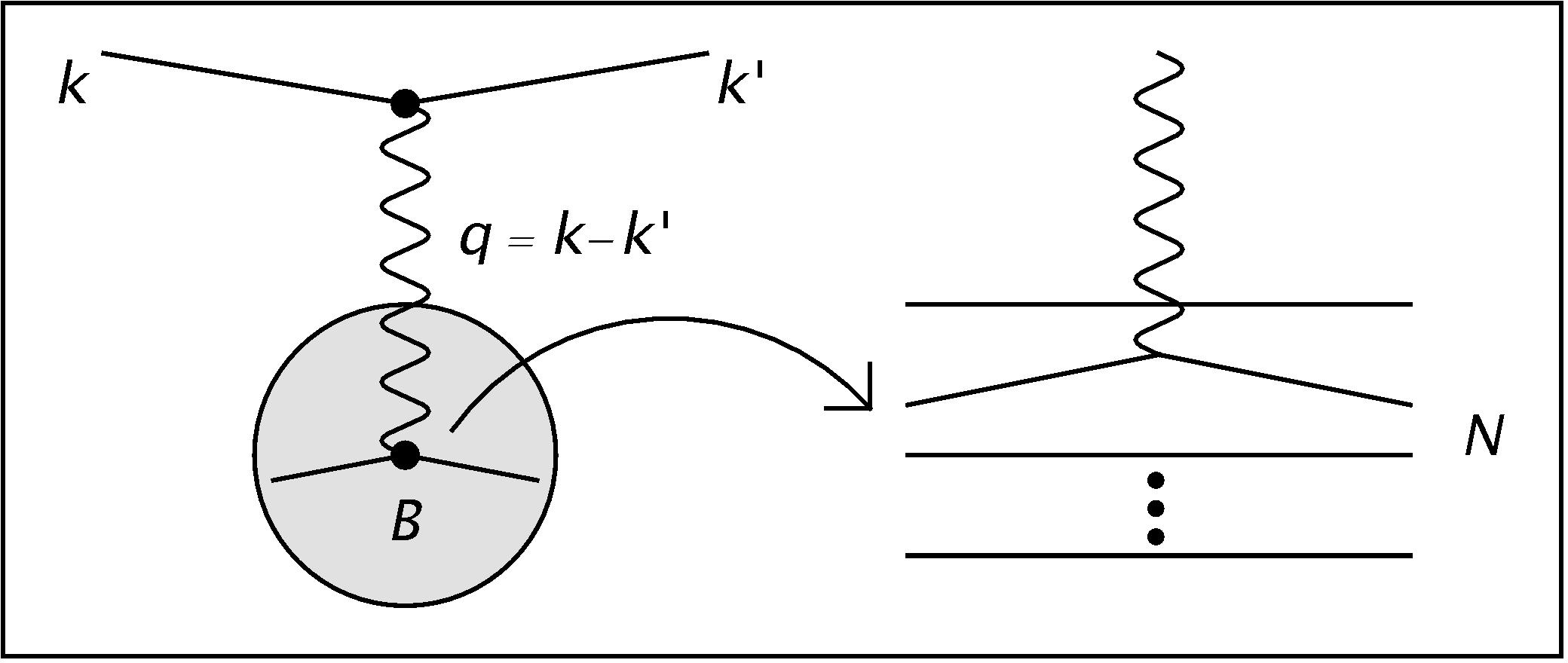
Figure 1: Feynman diagram for the scattering of a scalar on a black hole bound state at tree level. The wiggly line corresponds to the exchange of a virtual graviton. On the right hand side, the corresponding absorption is resolved into the microscopic constituents spectating and participating in the scatter process.

Before truncating ingoing and outgoing emitter legs, the one–graviton exchange amplitude for this process at tree level reads (Figure 1)

$$a^{(2)}(x_{1},x_{2})=\tfrac{{\rm i}^{2}}{M_{\rm P}^{\;4}}\int{\rm d}^{4}z_{1}{\rm d}^{4}z_{2}\;\mathcal{P}^{\mu\nu}(z_{1},z_{2};x_{1},x_{2})\mathcal{N}_{\mu\nu}(z_{2}),$$

where $\mathcal{P}$ contains all correlations with respect to the perturbative vacuum state $|0\rangle$, and $\mathcal{N}$ carries local, non-perturbative information about the black hole quantum state $|\mathcal{B}\rangle$:

$$\mathcal{P}^{\mu\nu} = \langle 0|{\rm T}\Phi(x_{2})\mathcal{T}_{\alpha\beta}(z_{1})\Phi(x_{1})|0\rangle\;\Delta^{\alpha\beta\mu\nu}(z_{1},z_{2})\;,$$

$$\mathcal{N}_{\mu\nu} = \langle\mathcal{B}^{\prime}|:\mathcal{T}_{\mu\nu}:(z_{2})|\mathcal{B}\rangle\;.$$ (8)

Here $\Delta$ denotes the free graviton propagator, and $|\mathcal{B}^{\prime}\rangle$ is the black hole quantum state after absorbing the graviton. Basically, $\mathcal{P}$ describes space–time events that originate outside the bound state, while $\mathcal{N}$ is localised in its interior.

Using the auxiliary current description, and provided that the bound state wave function $B(\mathcal{L})$ has a sufficiently compact support in $\mathcal{L}$–space, the graviton absorption event can be translated to the origin:

$$\mathcal{N}(z_{2})\approx{\rm e}^{-{\rm i}(P^{\prime}-P)\cdot z_{2}}\langle\mathcal{B}^{\prime}|:\mathcal{T}:(0)|\mathcal{B}\rangle\;,$$ (9)

with $P^{\prime}$ and $P$ denoting the black hole momentum after and before the graviton absorption, respectively, around which the corresponding wave function is peaked. The evaluation of $\mathcal{P}$ is straightforward. Truncating the ingoing and outgoing emitter legs, the one–graviton exchange amplitude becomes

$$\langle\mathcal{B}^{\prime}\Phi^{\prime}|\mathcal{B}\Phi\rangle^{(2)} =-{\rm i}(2\pi)^{4}\delta(k^{\prime}+P^{\prime}-k-P)\;\alpha_{\rm g}^{\;2}$$ (10)

$$\times\langle\mathcal{B}^{\prime}|:\mathcal{T}_{\mu\nu}:(0)|\mathcal{B}\rangle\;\Delta^{\mu\nu\alpha\beta}(k^{\prime}-k)\;G_{\alpha\beta\rho\sigma}\;\tfrac{k^{\prime\rho}k^{\sigma}}{k^{\prime 0}k^{0}}\;,$$

where the coupling $\alpha_{\rm g}\equiv 1/(4\pi M_{\rm P}^{\;2})$ has been introduced, and $G_{\alpha\beta\rho\sigma}=\eta_{\beta(\alpha}\eta_{\rho)\sigma}-\eta_{\beta\sigma}\eta_{\alpha\rho}$ is the Wheeler–DeWitt metric.

The total cross section $\sigma(\mathcal{B}^{\prime}\Phi^{\prime}\leftarrow\mathcal{B}\Phi)$ involves the absolute square of this amplitude and an integration over all intermediate bound states in the spectrum of the theory. Therefore, the differential cross section can be written as

$$k^{\prime 0}\frac{{\rm d}\sigma}{{\rm d}^{{}^{3}}k^{\prime}}=\frac{2}{\mathcal{F}(\Phi)}\;\left|\alpha_{\rm g}\Delta(k^{\prime}-k)\right|^{2}\;\mathcal{E}^{\alpha\beta\mu\nu}(k,k^{\prime})\mathcal{A}_{\alpha\beta\mu\nu}(\mathcal{B};k,k^{\prime})\;.$$ (11)

Here, $\mathcal{F}$ denotes the ingoing flux factor and $\Delta$ the scalar part of the graviton propagator. The emission tensor $\mathcal{E}$ captures the virtual graviton emission outside of the black hole, and the absorption tensor $\mathcal{A}$ its subsequent absorption by a black hole constituent. The emission tensor $\mathcal{E}\equiv Q\otimes Q$ is build from

$$Q^{\mu\nu}=4\pi^{2}\;\Pi^{\mu\nu\alpha\beta}(k^{\prime}-k)\;G_{\alpha\beta\rho\sigma}\;\tfrac{k^{\prime\rho}k^{\sigma}}{k^{\prime 0}k^{0}}\;,$$ (12)

with the graviton polarisation tensor $\Pi_{\mu\nu\alpha\beta}(q)\equiv\pi_{\mu(\alpha}\pi_{\beta)\nu}-\pi_{\mu\nu}\pi_{\alpha\beta}$, where $\pi_{\mu\nu}\equiv\eta_{\mu\nu}-\frac{q_{\mu}q_{\nu}}{q^{2}}$, and $k,k^{\prime}$ the on–shell momenta of the ingoing and outgoing scalar emitter, respectively. Graviton absorption is described as the energy momentum correlation of black hole constituents:

$$\mathcal{A}=\tfrac{1}{2\pi}\int{\rm d}^{4}x\;{\rm e}^{-{\rm i}(k^{\prime}-k)\cdot x}\langle\mathcal{B}|\mathcal{T}(x)\otimes\mathcal{T}(0)|\mathcal{B}\rangle\;.$$ (13)

Clearly, $\mathcal{A}$ contains information about the black hole interior, which is not yet resolved in terms of chronologically ordered subprocesses. For practical calculations, $\mathcal{A}$ will be related to the corresponding time ordered amplitude in the next section.

4 Chronological Ordering

Given that the graviton absorption tensor is not directly subject to time ordering, the question arises whether it can be deconstructed into causal correlations. The method to achieve this is very well-known in the context of scattering processes on bound states in QCD and will be adapted to the problem at hand in the following discussion.

As a first step, let us relate $\mathcal{A}$ to a tensor built from $\mathcal{T}(x)\wedge\mathcal{T}(0)$. Inserting a complete set of physical states in between the energy–momentum tensors at $x$ and $0$ in (13), and making good use of space–time translations, we arrive at

$$\mathcal{A}=\tfrac{1}{2\pi}\int\sum_{\mathcal{B^{\prime}}}(2\pi)^{4}\delta(q+P-P^{\prime})\langle B|\mathcal{T}(0)|\mathcal{B}^{\prime}\rangle\langle\mathcal{B}^{\prime}|\mathcal{T}(0)|\mathcal{B}\rangle\;,$$

with $q\equiv k-k^{\prime}$, $P$ and $P^{\prime}$ denoting the central momenta of wave–packets corresponding to ingoing and outgoing black hole quantum states, respectively. Standard kinematical arguments allow to replace (13) with

$$\mathcal{A}=\tfrac{1}{2\pi}\int{\rm d}^{4}x\;{\rm e}^{{\rm i}q\cdot x}\langle\mathcal{B}|[\mathcal{T}(x),\mathcal{T}(0)]|\mathcal{B}\rangle\;.$$ (14)

The absorption tensor (14) is given by the absorptive part of the Compton–like amplitude $\mathcal{C}$ for the forward scattering of a virtual graviton off a black hole,

$$\mathcal{C}={\rm i}\int{\rm d}^{4}x{\rm e}^{{\rm i}q\cdot x}\langle\mathcal{B}|{\rm T}\;\mathcal{T}(x)\otimes\mathcal{T}(0)|\mathcal{B}\rangle\;.$$ (15)

In order to see this, let us make the discontinuity of $\mathcal{C}$ manifest repeating the steps that allowed to extract the kinematical support of $\mathcal{A}$, leading to

$$\mathcal{C}=\int\sum_{\mathcal{B^{\prime}}}\tfrac{(2\pi)^{3}\delta({\bf P^{\prime}}-{\bf P}-{\bf q})}{P^{\prime 0}-P^{0}-q^{0}-{\rm i}\varepsilon}\langle\mathcal{B}|\mathcal{T}(0)|\mathcal{B}^{\prime}\rangle\langle\mathcal{B}^{\prime}|\mathcal{T}(0)|\mathcal{B}\rangle\;.$$ (16)

Defining Abs $\omega^{-1}\equiv[(\omega-{\rm i\varepsilon})^{-1}-(\omega+{\rm i\varepsilon})^{-1}]/(2{\rm i})$, it follows that Abs$(P^{\prime 0}-P^{0}-q^{0}-{\rm i}\varepsilon)^{-1}=\pi\delta(P^{\prime 0}-P^{0}-q^{0})$ and hence,

$$\pi\mathcal{A}(\mathcal{B};q)={\rm Abs}\;\mathcal{C}(\mathcal{B};q)\;,$$ (17)

which allows to deconstruct $\mathcal{A}$ in terms of chronologically ordered correlations.

5 Constituent representation of $\mathcal{A}$

In this section we give a physical interpretation of the absorption tensor in terms of constituent observables.

The time–ordered product of energy–momentum tensors in $\mathcal{C}$ gives rise to three contributions: The first corresponds to maximal connectivity between the tensors, resulting in a purely perturbative contribution void of any structural information. The second represents a disconnected contribution. Finally, the third contribution allows for perturbative correlations between the energy–momentum tensors and, in addition, carries structural information. Dropping the contributions void of structural information,

$${\rm T}\;\mathcal{T}_{\alpha\beta}(x)\mathcal{T}_{\mu\nu}(0)=\tfrac{1}{4}G_{\alpha\beta}^{ab}G_{\mu\nu}^{mn}\;C_{bm}(x)\;\mathcal{O}_{an}(x,0)\;,$$

where $C(x)\equiv 4\langle 0|{\rm T}\;{\rm d}\Phi(x)\otimes{\rm d}\Phi(0)|0\rangle$ denotes the correlation with respect to the perturbative vacuum,

$$C(x)=-\frac{2}{\pi^{2}}\frac{x^{2}\eta-4x\otimes x}{(x^{2})^{3}}$$ (18)

in free field theory, and $\mathcal{O}(x,0)\equiv\;:{\rm d}\Phi(x)\otimes{\rm d}\Phi(0):$ is the bi–local operator allowing to extract certain structural information when anchored in a quantum bound state.

In order to extract local observables, $\mathcal{O}(x,0)$ has to be expanded in a series of local operators. In principal this amounts to a Laurent–series expansion of the corresponding Green function. Let us first focus on its Taylor part:

$$\Phi(x)={\rm exp}\left(x\cdot\partial_{z}\right)\Phi(z)|_{z=0}\;.$$ (19)

The ordinary partial derivative is appropriate in the free field theory context, otherwise $\mathcal{O}(x,0)$ requires a gauge invariant completion. Then,

$$\mathcal{O}(x,0)=\sum_{j=0}^{\infty}\tfrac{1}{j!}\;\mathcal{O}^{[j]}(0)\;,$$ (20)

with $\mathcal{O}^{[j]}(0)\equiv\;:(x\cdot\partial_{z})^{j}{\rm d}\Phi(0)\otimes{\rm d}\Phi(0):$ and $[j]\equiv j+4$ denotes the mass dimension of the local operator. Note that we suppressed the space–time point $x$ appearing in the directional derivative in order to stress the local character of the operator expansion.

The fast track to relate $\mathcal{C}$ to constituent observables is to evaluate $\mathcal{O}(x,0)$ in a black hole quantum state using the auxiliary current description. We find for the local operators

$$\langle\mathcal{B}|\mathcal{O}^{[j]}(0)|\mathcal{B}\rangle=\kappa\left(x\cdot P\right)^{j}\langle\mathcal{B}|\Phi(r)\Phi(0)|\mathcal{B}\rangle P\otimes P\,.$$ (21)

Here, $\kappa$ denotes a combinatoric factor. Note that a simple point–split regularisation has been employed ($r^{2}\rightarrow 0$). The operator appearing on the right hand side of (21) measures the constituent number density.

Hence, the absorptive part of the forward virtual graviton scattering amplitude $\mathcal{C}$ or, equivalently, the graviton absorption tensor $\mathcal{A}$ can be directly interpreted in terms of the black hole constituent distribution.

6 Analytic properties of $\mathcal{C}$

The Ward–Takahashi identity associated with the underlying gauge symmetry fixes the tensorial structure $\theta_{\alpha\beta\mu\nu}(q,P)\equiv\Pi_{\alpha\beta}^{ab}\Pi_{\mu\nu}^{mn}\eta_{bm}P_{a}P_{n}$ of the amplitude $\mathcal{C}(q,P)$ in accordance with source conservation. The Laurent–series expansion of $\mathcal{O}(x,0)$ in local operators gives to leading order up to $\mathcal{O}(q\cdot P/P^{2})$

$$\mathcal{C}(q,P) = \langle\mathcal{B}|\Phi(r)\Phi(0)|\mathcal{B}\rangle\;\theta(q,P)\;\tfrac{\rm-i}{2\pi^{2}}\sum_{j=-\infty}^{\infty}C_{j}(q)u^{j}\;.$$ (22)

Here, the coefficients $C_{j}$ are calculable and turn out to be momentum independent, and the expansion parameter $u\equiv-P^{2}/q^{2}\gg 1$. Note that this parameter is the analogue of the inverse Bjorken scaling variable known from deep inelastic scattering. There is a profound difference between these two parameters, however. While in standard discussions of deep inelastic scattering in the infinite momentum frame one makes use of asymptotic freedom, this is not possible in gravity. For the problem at hand, however, there is a natural limit and correspondingly an appropriate expansion parameter. Namely, considering black holes of large mass and momentum transfers smaller than $M_{\rm P}$ (which is needed in order to trust the perturbative expansion) we are naturally lead to the expansion parameter $u$.

The discontinuity of $\mathcal{C}$ for fixed $q^{2}=-Q^{2}$ is at

$$u_{*}=\tfrac{M_{\mathcal{B}}}{2(M_{\mathcal{B}}^{\prime}-M_{\mathcal{B}})}\left(1-\tfrac{M_{\mathcal{B}}^{\prime 2}-M_{\mathcal{B}}^{2}}{Q^{2}}\right)\gg 1\;.$$ (23)

So $\mathcal{C}$ has an isolated pole at $u_{*}\gg 1$ and, in particular, no branch cut in leading order, corresponding to the statement that $M_{\mathcal{B}}^{\prime}/M_{\mathcal{B}}-1\approx 0$. Of course, the presence of a branch cut beyond leading order poses no obstacle. On the contrary, it has an evident interpretation in terms of intermediate black hole excitations.

In order to project onto the Laurent–coefficients, a path enclosing $[-u_{*},u_{*}]\subset\mathbb{R}$ in the complex $u$ plane has to be chosen.

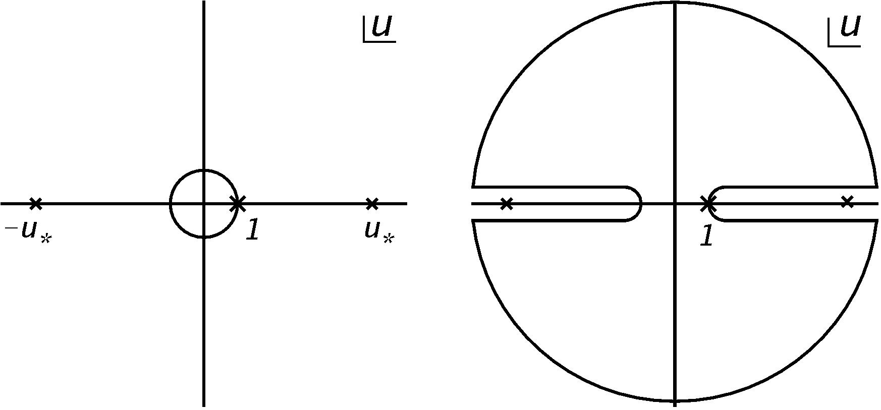
Figure 2: Integration contour in the complex $u$-plane. The left figure displays an integration contour corresponding to the radius of convergence. In order to relate this to the physical $u$-region ($P^{2}>Q^{2}$) we perform a contour deformation (right figure). The radius of the circle is sent to infinity.

This covers the physical $u$ region, while the radius of convergence of the corresponding Taylor series would only allow for unphysical $u\in[-1,1]$ (see Figure 2). We find

$$\int_{0}^{1}{\rm d}\zeta\;\zeta^{k-2}\mathcal{A}(q,P,\zeta)=\tfrac{C_{k-1}}{4\pi^{2}}\;\langle\mathcal{B}|\Phi(r)\Phi(0)|\mathcal{B}\rangle\;\theta(q,P)\;,$$ (24)

with $\zeta\equiv 1/u$ denoting the graviton virtuality relative to the black hole target mass. Hence, all moments of the absorption tensor with respect to $\zeta$ are directly proportional to the constituent distribution inside the black hole. This implies that ${\rm d}\sigma/{\rm d}^{3}k^{\prime}\propto\langle\mathcal{B}|\Phi(r)\Phi(0)|\mathcal{B}\rangle$. Thus, black hole constituent distributions are observables that can be extracted from scattering experiments.

Although $\langle\mathcal{B}|\Phi(r)\Phi(0)|\mathcal{B}\rangle$ can in practice not be determined from first principles, we will give a simple toy model for the wave function in the next section and compute $\mathcal{D}(|{\bf r}|)$. Requiring that the wave function is localized within the Schwarzschild radius (which seems to be a sensible assumption), will lead to a qualitative understanding of the distribution of quanta inside $|\mathcal{B}\rangle$.

In order to allow quantitative statements this means that the distribution should be measured at some scale $\Lambda\ll M_{\rm{p}}$ where the effective field theory description is valid. Predicting the cross section at a different scale can then be achieved by means of renormalization group techniques. Notice that this procedure is similar to the DGLAP evolution of quark and gluon distributions within the framework of perturbative QCD. Renormalization group evolution, however, will be studied in future work.

7 Constituent distribution at parton level

In Sections 5 & 6 we presented a constituent interpretation for virtual graviton absorption by a black hole quantum bound state. Central for this interpretation was the constituent distribution $\mathcal{D}(r)\equiv\langle\mathcal{B}|\Phi(r)\Phi(0)|\mathcal{B}\rangle$. As discussed in Section 2, $\mathcal{D}(r)$ can only depend on the spatial distance $|{\bf r}|$, but not on time.

The spatial length scale $|{\bf r}|$ is at the observers disposal. It can be interpreted as the necessarily finite spatial extent of an apparatus that emits a $\Phi$ quantum at one end and subsequently absorbs it at the other end. In between emission and absorption the quantum probes the medium in which the apparatus has been submerged, in our case the black hole interior. At the partonic level, no individual interactions between the probe and black hole constituents take place, therefore the only relevant scale remains $|{\bf r}|$. Effectively, then, there is only the correlation across the apparatus between emission and absorption events, which scales as $|{\bf r}|^{-2}$. The light–cone distribution of black hole constituents has been calculated in Hofmann at the parton level and to leading order in $1/N$. As explained in Hofmann these $1/N$–corrections already arise at the level of combinatorics associated to the diagrams that need to be computed. Note that these corrections are in accordance with the ideas of Dvali .

$$\mathcal{D}(|{\bf r}|)=2\Big{(}\frac{N}{M_{\mathcal{B}}}\Big{)}^{4}\Gamma_{\mathcal{B}}^{-2}\langle\Phi^{2(N-2)}\rangle\frac{1}{4\pi^{2}|{\bf r}|^{2}}\int d^{3}P\cos({\bf Pr}/2)|\mathcal{B}({\bf P},\mathcal{Q})|^{2},$$ (25)

where $\langle\Phi^{2(N-2)}\rangle$ is a condensate parametrizing the non–perturbative vacuum structure inside a black hole quantum bound state. At the diagrammatic level, $\mathcal{D}(|{\bf r}|)$ can be represented by Figure 3. Note that gauge corrections to (25) can be calculated following Hofmann .

Even in the absence of gauge interactions, $N$ carries non–perturbative information via its dependence on $\Gamma_{\mathcal{B}}$ and, in addition, its dependence on $\Phi$ condensates, see Hofmann . The latter dependence deserves elaboration. It can be traced back to the fact that $N\gg 1$ for black holes, implying minimal connectivity between the space–time events at which the auxiliary currents are operative.

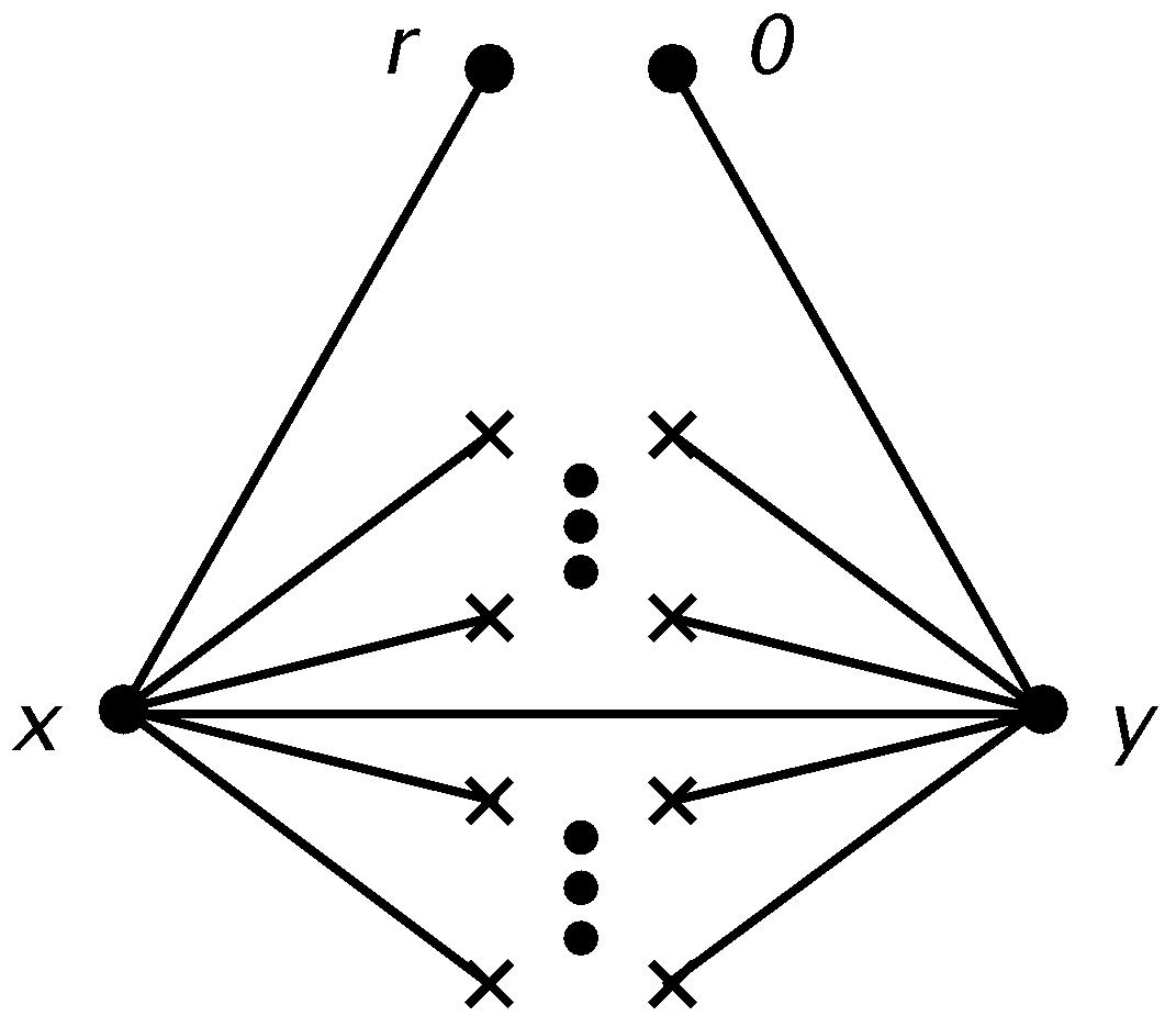
Figure 3: This is the only diagram contributing to $\mathcal{D}(|{\bf r}|)$. Straight lines represent free propagators, while lines ending in crosses correspond to non-perturbative condensation processes.

At the level of $\mathcal{D}(|{\bf r}|)$, this can be seen as follows. The constituent distribution is generated by a four–point correlator, where two space–time points are associated with the read–in events (auxiliary current locations) and one point–split for localising an apparatus of finite extent, consisting of an emitter and an absorber. The measurement process requires altogether six $\Phi$ fields at four space–time locations. The vast majority of fields composing the auxiliary currents has two options. Either they enhance the connectivity between the currents locations, or they condense. Condensation of $\Phi$ quanta turns out to be the favoured option in the so–called double scaling limit, $N,M_{\mathcal{B}}\rightarrow\infty$ and $N/M_{\mathcal{B}}=$const., where $M_{\mathcal{B}}$ denotes the bound state’s mass.

Violations of this limit are not exponentially suppressed, but of order $1/N\ll 1$, indicating the essential quantum character of black holes. Since the cross section is given in terms of the number density, these corrections are in principle measurable in scattering experiments.

Black holes naturally are large–$N$ quantum bound states. If operative as sources, they trivialize (planar dominance tHooft ; Witten ) the underlying quantum theory of constituent fields and represent an unrivalled realisation of the large–$N$ limit in nature.

Before concluding this section, let us calculate the constituent distribution $\mathcal{D}(|{\bf r}|)$ assuming a Gaussian wave function $\mathcal{B}({\bf P},\mathcal{Q})$ for the black hole peaked around $M_{\mathcal{B}}$ with a standard deviation given by $1/r_{\rm g}$. This choice reflects those features of the a priori unknown black hole state that are relevant for the qualitative behaviour of the constituent distribution. For instance, the non–perturbative ground state has compact support characterised by the size of the bound state itself. In Figure 4 we show the constituent distribution in wavelength space, $\widetilde{D}(\lambda)\propto\lambda\operatorname{erf}(2r_{\rm g}/\lambda)$, where $\operatorname{erf}$ denotes the error function and $\lambda=1/|{\bf k}|$. Here $|{\bf k}|$ is the absolute value of the constituent three–momentum. As can be seen, black hole constituents favour to occupy long wavelength modes. In other words, black hole interiors are dominated by soft physics in accordance with the postulates of reference Dvali .

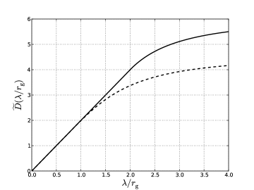
Figure 4: Parton distribution as a function of the wavelength for a gaussian wave function of variance $r_{\rm g}$ (dashed line) and a Heaviside profile (solid line). Here $\tilde{\mathcal{D}}(\lambda/r_{\rm g})$ is normalised to $\frac{r_{\rm g}}{2}(N/M)^{4}\Gamma_{\mathcal{B}}^{-2}\langle\Phi^{2(N-2)}\rangle$. The distribution is plotted only for wavelengths $\lambda<4r_{\rm g}$ since the condensates are not supported outside the black hole. By construction our analysis is valid only up to $\lambda=2r_{\rm g}$.

8 Discussion & Summary

Black holes are perhaps the most celebrated solutions of general relativity. Within our framework they are considered as bound states of quantum constituents on flat space–time with physical radius $r_{\rm g}$.

We discussed the representation of bound states in terms of currents in detail. Subsequently we specialised to spherically symmetric gravitating sources including black hole quantum bound states.

A quantum theory of black hole constituents allows to extract structural information from the associated quantum bound state. We showed that the process of virtual graviton absorption by a black hole is directly related to the constituent distribution inside the black hole. In particular, we gave a precise prediction for the differential scattering cross section of massless scalars on a black hole in terms of microscopic degrees of freedom constituting the bound state. Hence the constituent distribution is a faithful observable — it can be defined using a gauge invariant operator and, in addition, a scattering process can be specified allowing its measurement. Thus, in contrast to the standard lore, within our framework an outside observer in principle has access to the internal structure of a black hole.

We discussed the physics underlying graviton absorption by black holes. The quantum bound state proposal employed here is based on individually weakly coupled constituents immersed in a non–trivial medium. Constituent condensation is supported by a non–perturbative ground state $|\Omega\rangle$ and by the large–$N$ character of black holes. The quantum bound states associated with black holes can be generated by operating with an appropriate current $\mathcal{J}$ on $|\Omega\rangle$. These sources trivialise the underlying field theory and allow to consider black holes as the simplest realisations of large–$N$ bound states in nature. Finite $N$ effects can (and should) be studied, since they are not exponentially suppressed, proving that the bound state construction is truly quantum, and, consequently, that black holes are essentially beyond a semi–classical description. Furthermore, higher order radiative corrections to the scattering process leading to evolution equations for the distribution function should be considered in the future.

- (1) M. J. Duff, Quantum Tree Graphs and the Schwarzschild Solution, Phys. Rev. D 7, (1973) 2317.
- (2) M. A. Shifman, A. I. Vainshtein and V. I. Zakharov, QCD and Resonance Physics. Sum Rules, Nucl. Phys. B 47 (1979) 385.
- (3) M. A. Shifman, A. I. Vainshtein and V. I. Zakharov, QCD and Resonance Physics: Applications , Nucl. Phys. B 47 (1979) 448.
- (4) G. Dvali and C. Gomez, Black hole’s quantum N-portrait, Fortschr. Phys. 61 (2013) 742.
- (5) G. Dvali and C. Gomez, Black hole’s 1/N hair, Phys. Lett. B 719 (2013) 419.
- (6) G. ’t Hooft, A planar diagram theory for strong interactions, Nucl. Phys. B 72 (1974) 461.
- (7) E. Witten, Baryons in the 1/N expansion, Nucl. Phys. B 160 (1979) 57.
- (8) S. Hofmann, T. Rug, A Quantum Bound–State Description of Black Holes, (2014) arxiv:1403.3224 [hep-th]