Commensurate and Incommensurate States of Topological Quantum Matter

Abstract

We prove numerically and by dualities the existence of modulated, commensurate and incommensurate states of topological quantum matter in simple systems of parafermions, motivated by recent proposals for the realization of such systems in mesoscopic arrays. In two space dimensions, we obtain the simplest representative of a topological universality class that we call Lifshitz. It is characterized by a topological tricritical point where a non-locally ordered homogeneous phase meets a disordered phase and a third phase that displays modulations of a non-local order parameter.

In recent years, most efforts directed at investigating topological quantum matter experimentally have taken a top-to-bottom approach, starting from model Hamiltonians and engineering a systems to realize it. From this point of view, mesoscopic superconducting arrays have already been proven successful ioffe09 , and also for cold atomic gases the implementation of topological phases of matter seems within reach goldman13 .

Inevitably, the model Hamiltonians in question can only be realized up to implementation-dependent modifications, that, although small, may be relevant in the sense of the renormalization group and drive large systems away from the intended topological phase. This practical aspect of the theory of phase transitions for topological quantum matter is the natural counterpart of analogous considerations for conventional systems like magnetic memories, which can only tolerate some range of temperatures and applied magnetic fields. However there is one crucial difference. Since a Landau theory of non-local order parameters, which are those appropriate to topological quantum matter, does not exist yet, it is difficult to predict and classify interacting topological gapless phases. By contrast, the classification of gapped phases is understood (for parafermions, see Bondesan2013 ; Motruk2013 ).

In this paper we extend the list of demonstrated topological critical behaviors (see, for example, Ardonne2004 ; Feiguin2007 ; Tupitsyn2010 ; Dusuel2011 ; Schulz2012 ). We will show that topological quantum matter can be driven into phases characterized by non-local orders incommensurate with the underlying lattice. Remarkably, it will become clear that modulated and floating (and, in particular, incommensurate) topological quantum orders can easily arise in mesoscopic arrays from very natural interactions. And we will prove the existence of a topological universality class surprisingly sensitive to an underlying lattice structure by locating a topological Lifshitz tricritical point in the phase diagram of a two-dimensional model of topological quantum matter.

But let us recall first the basics of modulated Landau orders. When a local order parameter $\Phi({\bm{x}})$ emerges in a lattice system, phases may occur in which this order parameter displays modulations $\Phi({\bm{x}})\sim\Phi_{0}\cos({\bm{k}}_{0}\cdot{\bm{x}}+\phi_{0})$ commensurate with the lattice periodicity. The wave vector ${\bm{k}}_{0}$ is restricted by the Lifshitz condition to take one of a few possible values in the first Brillouin zone Landau1968 .

This picture of modulated local orders can break down if interactions that favor competing periodicities are present, as exemplified by the ANNNI model Bak1982 ; Selke1988 of magnetic ordering in the heavy lanthanoids Elliott1961 . In systems with such competing interactions, there might be regimes where the equilibrium wave vector varies continuously with some driving force, as first predicted in Ref. Hornreich1975 from the Landau functional density

$$f=\kappa_{2}\Phi^{2}+\kappa_{4}\Phi^{4}+\kappa_{6}\Phi^{6}+\gamma_{1}(\nabla\Phi)^{2}+\gamma_{2}(\nabla^{2}\Phi)^{2}$$ (1)

for an Ising order parameter. Just as the standard Ising tricritical point emerges at $\kappa_{2}=\kappa_{4}=0$, the Lifshitz tricritical point emerges at $\gamma_{1}=0$. It is the coexistence point for the paramagnetic, ferromagnetic, and modulated phases of the local order parameter $\Phi$. On the coexistence line between the modulated and paramagnetic phases, starting at the Lifshitz point, the wave vector ${\bm{k}}$ varies continuously with the driving field and so an additional critical exponent appears. If ${\bm{k}}$ happens to vary continuously in a phase, then the phase is called floating.

In the following we demonstrate through explicit examples that the full range of phenomena associated with commensurate and incommensurate modulations and the Lifshitz point can also be present in topological quantum matter, but now in terms of non-local order parameters. Unlike the situation for local (Landau) orders just discussed, there is no obvious way to predict such topological quantum orders on the basis of some general Landau-Wilson functional. This point showcases one of the troubling limitations in our current understanding of topological quantum matter at criticality.

We start by considering a one-dimensional effective Hamiltonian with a discrete global $\mathbb{Z}_{2m}$ ($m=1,3,\dots$ odd) symmetry that displays a critical floating phase. One may obtain a $\mathbb{Z}_{2m}$ symmetry in systems with quasiparticles of fractional charge $e/m$ subjected to proximity-induced superconducting pairing. The combination of these two ingredients provides a channel for Cooper pairs to split into $2m$ indistinguishable parts. Then the condensation of the Cooper pairs leads to a peculiar cyclic behavior of the local, charged degrees of freedom and induces the required $\mathbb{Z}_{2m}$ symmetry. These ideas are central to several proposals stern2012 ; shtengel2012 ; vaezi2013 ; cheng2013 that aim to realize localized parafermionic zero-energy modes (parafermions for short) in hybrid mesoscopic arrays including fractional topological insulators (FTI). Parafermions are obtained by gapping the edge modes of a FTI and constitute a fractionalized version of Majorana zero-energy edge modes (Majoranas for short), allowing for the emergence of 1D systems which generalize fendley2012 ; Bondesan2013 ; Motruk2013 ; Cobanera2014 ; Li2014 the well-known Majorana-Kitaev chain kitaev2001 .

Along the edge of an FTI, localized parafermions emerge at the interfaces between alternating regions where the edge modes of the FTI are gapped by proximity to superconducting islands or insulating ferromagnets stern2012 ; shtengel2012 , see Fig. 1. Each superconducting island $i$ hosts a pair of parafermionic modes $\Gamma_{i},\Delta_{i}$ sharing a fractional charge $q_{i}^{\sf f}=0,\frac{1}{m},\frac{2}{m},\ldots,\frac{2m-1}{m}$, in units of $e$, defined modulo $2$ stern2012 ; shtengel2012 . Parafermions obey non-local commutation rules,

$$\Gamma_{i}\Delta_{j} = e^{{\sf i}\frac{\pi}{m}}\,\Delta_{j}\Gamma_{i}\quad(i\leq j),$$ (2)

$$\Gamma_{i}\Gamma_{j} = e^{{\sf i}\frac{\pi}{m}}\,\Gamma_{j}\Gamma_{i},\quad\Delta_{i}\Delta_{j}=e^{{\sf i}\frac{\pi}{m}}\Delta_{j}\Delta_{i}\quad(i<j),$$ (3)

$$\Gamma_{i}^{2m} = \mathds{1}=-\Delta_{i}^{2m},\quad\Gamma_{i}^{\;}\Gamma_{i}^{\dagger}=\Delta_{i}^{\;}\Delta_{i}^{\dagger}=\mathds{1}.$$ (4)

This algebra of parafermions is a natural generalization of the Clifford algebra of Majoranas.

The charge $q_{i}^{\sf f}$ is the charge of the FTI edge segment coupled to the superconductor and may be represented by the operator $\Gamma_{i}^{\dagger}\Delta_{i}=e^{i\pi q_{i}^{\sf f}}$. In our mesoscopic array, two main physical processes intervene to couple the zero-energy modes: a fractional Josephson effect shtengel2012 ; cheng2013 , which generalizes the electron tunneling mediated by Majorana modes xu2010 , and the charging interactions of the islands which, just like in the Majorana case vanheck2011 ; vanheck2012 ; hassler2012 , cause an energy splitting of the states with different fractional charges Burrello2013 . The Josephson interaction accounts for the tunneling of fractional quasiparticles between two neighboring islands and it changes their fermionic number by $\pm 1/m$. The tunneling of a single fractional charge is the dominant process and, in terms of parafermionic modes, it reads $-\left({E_{J}}/{2}\right)(\Gamma_{i+1}\Delta_{i}^{\dagger}+H.c.).$ The charging interactions are modelled by assuming that each island is coupled to a background superconductor by a strong normal Josephson junction and a capacitive contact, with magnitudes $\varepsilon_{J}$ and $\varepsilon_{C}$ respectively. See Fig. 1.

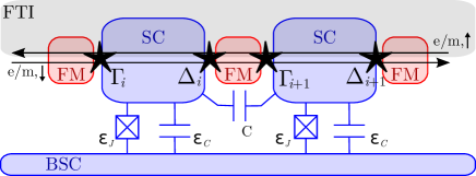
Figure 1: Parafermions $\Gamma_{i}$ and $\Delta_{i}$ are localized along the edge of a FTI at the interfaces between superconducting islands (SC) and insulating ferromagnets (FM). Each superconducting island is coupled to neighboring islands via a capacitive coupling $C$, and to a ground superconductor (BSC) via a Josephson junction $\varepsilon_{J}$ and a capacitive coupling $\varepsilon_{C}$.

Besides the contribution coming from Cooper pairs, the total charge in each island includes the charge $q^{\sf ind}_{i}$ induced by the neighboring potentials, and the fractional charge $q_{i}^{\sf f}$ associated to the parafermions. The effect of these two contributions is especially important if $\varepsilon_{J}\gg\varepsilon_{C}$, that is, in the transmon regime girvin07 . In this regime the low energy physics can be described by semiclassically assuming that the superconducting phase of the island is approximately pinned to the minima of the Josephson energy. Then the charging energy causes an effective interaction $-\Delta_{C}\cos\left(\pi(q^{\sf f}_{i}+q^{\sf ind}_{i})\right)$, where $\Delta_{C}$ depends on the ratio $\varepsilon_{J}/\varepsilon_{C}$ girvin07 , and the cosine dependence is due to the Aharonov-Casher effect associated with $2\pi$-phase slips in states with different charges $q^{\sf f}_{i}+q^{\sf ind}_{i}$ vanheck2011 ; hassler2012 . Following Burrello2013 , this interaction may be written as $-({1}/{2})\left(E_{C}^{(1)}\Gamma_{i}^{\dagger}\Delta_{i}+H.c.\right),$ where $E_{C}^{(1)}=\Delta_{C}e^{-{\sf i}\pi q^{\sf ind}}$ is, in general, complex. It is possible to tune $q^{\sf ind}$, using voltage gates in the system, to take the values $0$ or $1$ and thus obtain a positive or negative single-island charging energy term.

A further charging term appears in the presence of a cross-capacitance $C$ between neighboring islands. This term originates from the simultaneous $2\pi$-phase slip of both islands hassler2012 and reads $-E^{(2)}_{C}\cos\left(\pi(q_{i}^{\sf f}+q_{i+1}^{\sf f}+q^{\sf ind}_{i}+q^{\sf ind}_{i+1})\right)$. In particular, we impose that all the induced charges share a common value $q^{\sf ind}$. By tuning $q^{\sf ind}$ to add a unit of charge to each island ($q^{\sf ind}_{i}\to q^{\sf ind}_{i}+1$), the relative sign between the coupling strengths $E^{(1)}_{C}$ and $E^{(2)}_{C}=|E_{C}^{(2)}|e^{-{\sf i}2\pi q_{\sf ind}}$ may be controlled. This cross-capacitance interaction is translated into a four-parafermion operator and, combining all the previous terms, we obtain an effective Hamiltonian

$$H_{\sf eff} = -\frac{1}{2}\sum_{i=1}^{L}[(E_{J}\Gamma_{i+1}\Delta_{i}^{\dagger}$$

$$+ E^{(1)}_{C}\Gamma_{i}^{\dagger}\Delta_{i}+E_{C}^{(2)}\Gamma_{i}^{\dagger}\Delta_{i}\Gamma_{i+1}^{\dagger}\Delta_{i+1})+H.c.]$$

for the description of the array of Fig. 1 in its low-energy sector with periodic boundary conditions. In the following, we will take $E^{(1)}_{C}=1$ and $E_{C}^{(2)}\leq 0$. Then $H_{\sf eff}$ is closely connected to a generalization of the ANNNI model (corresponding to $m=1$) to any odd $m$ supplemental_material .

Figure 2: Quantum phase diagram of $H_{\sf eff}$ for $m=3$. The three ordered phases are labeled by the wave vector associated to the modulation of the string order parameter. The disordered phase contains modulated and unmodulated regimes, separated by the (dashed) disorder line. There are two critical phases with central charge $c=1$. Various indicators were used to mark the transitions: Blue dots mark global maxima of the entanglement entropy, green stars mark local maxima of its first $E_{J}$ derivative, red upwards triangles mark local minima of the second $E_{J}$ derivative of the ground energy, and black triangles mark discontinuities in the first derivative of the ground energy.

We studied the quantum phase diagram of $H_{\sf eff}$ for $m=3$ numerically, computing approximate ground states using the open source evoMPS toolbox evoMPS , which implements variational tangent plane techniques for matrix product states (MPS) tangent_plane_mps . In particular, evoMPS implements the nonlinear conjugate gradient method to accelerate the process significantly, particularly for critical regimes, in comparison to imaginary time evolution Milsted2013 . We choose block translation invariant MPS with various block lengths in order to handle ground states with nontrivial periodicity.

The quantum phase diagram of $H_{\sf eff}$ is shown in Fig. 2. There are three distinct gapped phases at low $E_{J}\geq 0$ followed by two critical phases, both with central charge $c=1$ mps_cc . The critical phases are topped by a gapped phase at large $E_{J}$. To further characterize the (dis)orders in these phases, we follow the ideas of Refs. Cobanera2013 ; vanHeck2014 to determine a non-local order parameter for $H_{\sf eff}$ by mapping this Hamiltonian to a Landau-ordered system. We obtain supplemental_material that the ground-state $|\Omega\rangle$ expectation value

$$\Sigma_{i}(d)=\langle\Omega|\prod_{n=i}^{i-d+1}\Gamma_{n}^{\dagger}\Delta_{n}^{\;}|\Omega\rangle$$ (6)

(independent of $i$) defines the required non-local order parameter. The string order parameter $\Sigma_{i}(d)$ displays long-range order in the three gapped phases at small $E_{J}$, with modulations characterized by $k_{0}=0,\pi/3,\pi/2$. The wave vectors are ordered as they appear for increasing $-E^{(2)}_{C}$, see Fig. 2. The ordered phases with $k_{0}=0,\pi/3$ are separated by a first-order line.

Starting at $E_{J}=0$ in either the gapped phase with $k_{0}=\pi/3$ or $k_{0}=\pi/2$ and increasing $E_{J}$ along a vertical line, the system enters the critical phase on the right in Fig. 2, and the asymptotic behavior of $\Sigma_{i}(d)$ changes from long-ranged to algebraically decaying, but with a modulation $k_{0}(E_{J})$ that appears to vary continuously with $E_{J}$ to the best available computer resolution. In this regime, the periodicity of the non-local order in the system is no longer anchored to the lattice structure, and so our mesoscopic array demonstrates the existence of floating regimes for mesoscopically-realized topological quantum matter. Fig. 3 shows $k_{0}(E_{J})$ for the full range of $E_{J}$ for three values of $-E^{(2)}_{C}$ starting at $k_{0}=\pi/3$, and two values starting at $k_{0}=\pi/2$.

As for the other phases, $\Sigma_{i}(d)$ shows no modulations in the critical phase on the left of the phase diagram. At $-E^{(C)}_{2}=0$, this phase is precisely supplemental_material the critical phase of the $p=2m=6$ clock model (see clock and references therein). The modulations of the string order parameter survive in the the gapped, disordered phase at large $E_{J}$ where $\Sigma_{i}(d)$ decays exponentially fast in $d$, but only for sufficiently large values of $-E^{(2)}_{C}$. There is a regime in the disordered phase without modulations, as shown in Fig. 2. The separation between the two disordered regimes, unmodulated and modulated, is called the disorder line in the literature on the ANNNI model.

Figure 3: Fitting of $\mathrm{Re}({\Sigma_{i}(d)})$ with a decay function modulated with wave vector $k_{0}$. The wave vectors starts at a constant value in the ordered phases and change continuously in the the critical phase on the right of the phase diagram. The error bars represent statistical errors from the least-squares fitting.

The string-ordered phases of $H_{\sf eff}$ manifest the various ways in which the global, discrete symmetry

$$U_{\sf C}=\prod_{i=1}^{L}\Gamma_{i}^{\dagger}\Delta_{i},\quad U_{\sf C}^{2m}=\mathds{1},\quad\left[U_{\sf C},H_{\sf eff}\right]=0\,,$$ (7)

can be spontaneously broken in the limit of infinite system size. There are however topological quantum orders that emerge without spontaneously breaking any symmetries, as first noticed for Ising gauge theories Wegner1971 . These states of topologically quantum matter are often modelled by systems with local symmetries, since, by Elitzur’s theorem Elitzur1975 , local symmetries cannot be spontaneously broken. The remainder of the paper focuses on a model that displays incommensurate behavior, and even a full-fledged topological Lifshitz point, without spontaneous symmetry breaking. We call a Lifshitz point topological if it is a tricritical point of the Lifshitz type, but associated to non-local orders only.

The model in question, inspired by the mesoscopic realization of the toric code in terms of Majoranas Terhal2012 , features parafermions $\Gamma_{({\bm{r}},\mu)},\Delta_{({\bm{r}},\mu)}$ ($\mu=1,2$) on each link $({\bm{r}},\mu)$ connecting sites ${\bm{r}},{\bm{r}}+\bm{e_{\mu}}$ of a square lattice. Let us define plaquette operators $B_{\bm{r}}=U_{({\bm{r}},1)}U_{({\bm{r}}+{\bm{e_{1}}},2)}U_{({\bm{r}}+{\bm{e_{2}}},1)}^{\dagger}U_{({\bm{r}},2)}^{\dagger}$ (in terms of the shorthand notation $U_{({\bm{r}},\mu)}=\Gamma_{({\bm{r}},\mu)}^{\dagger}\Delta_{({\bm{r}},\mu)}$), and star operators $A_{\bm{r}}=\Delta_{({\bm{r}},1)}\Gamma_{({\bm{r}}-{\bm{e_{2}}},2)}^{\dagger}\Delta_{({\bm{r}},2)}\Gamma_{({\bm{r}}-{\bm{e_{1}}},1)}^{\dagger}.$ As the naming suggests, the star and plaquette operators generate a commutative algebra. The gapped Hamiltonian

$$H_{\sf TC}=-\frac{1}{2}\sum_{\bm{r}}[h_{p}B_{\bm{r}}+h_{s}A_{\bm{r}}+H.c.]$$ (8)

is precisely the parafermionic representation of the $\mathds{Z}_{2m}$ toric code. In the following we will study the effect of the perturbation

$$V=-\frac{J_{1}}{2}\sum_{{\bm{r}},\mu}[U_{({\bm{r}},\mu)}+H.c.]-\frac{J_{2}}{2}\sum_{\bm{r}}[U_{({\bm{r}},2)}U_{({\bm{r}}+{\bm{e_{1}}},2)}+H.c.]$$ (9)

with $J_{1},-J_{2}\geq 0$. Since the plaquette operators $B_{\bm{r}}$ commute with the full Hamiltonian $H_{\sf LTC}=H_{\sf TC}+V$, they play the role of local symmetries. The ground state of the system belongs to the gauge-invariant sector where the plaquettes $B_{\bm{r}}$ act as the identity.

For the purpose of realizing the topological Lifshitz universality class, it suffices to consider only the simplest case of $m=1$ for which the parafermions reduce to Majoranas. Following Cobanera2014 , we exploit a gauge-reducing duality transformation Cobanera2011 to map $H_{\sf LTC}$ to a dual Landau-ordered system $H_{\sf LTC}^{D}$. Because we fix $m=1$, this dual system features spins $S=1/2$ placed at the sites ${\bm{r}}$ of a square lattice, represented by Pauli matrices $\sigma^{\alpha}_{\bm{r}}$. It is governed by the Hamiltonian

$$H_{\sf LTC}^{D}= - \sum_{\bm{r}}(h_{s}\sigma^{x}_{\bm{r}}+h_{p}\mathds{1})$$

$$- J_{1}\sum_{{\bm{r}},\mu}\sigma^{z}_{\bm{r}}\sigma^{z}_{{\bm{r}}-\bm{e_{\mu}}}-J_{2}\sum_{\bm{r}}\sigma^{z}_{{\bm{r}}-{\bm{e_{1}}}}\sigma^{z}_{{\bm{r}}+{\bm{e_{1}}}}.$$

The dual Hamiltonian $H_{\sf LTC}^{D}$ is precisely the celebrated quantum ANNNI model in two space dimensions. In mean field, $H_{\sf LTC}^{D}$ is directly connected to the Landau functional of Eq. (1) Selke1988 . Since dualities are unitary transformations Cobanera2011 , we obtain that our perturbed toric code and the ANNNI model share identical phase diagrams. In the following we rely on the extensive knowledge of this phase diagram collected in Ref. Selke1988 .

To characterize the non-local (dis)orders in the quantum phase diagram as it pertains to the topological model $H_{\sf LTC}$, we need to identify a non-local order parameter. Again, we follow the ideas of Ref. Cobanera2013 and obtain supplemental_material the string order parameter

$$\Sigma_{\bm{r}}(d)=\langle\Omega|\prod_{j=1}^{d}U_{({\bm{r}}+j{\bm{e_{1}}},2)}|\Omega\rangle.$$ (11)

In terms of $h_{s}$ versus $-J_{2}/J_{1}$, the phase diagram splits into a phase at high $h_{s}$ with exponential decay of the string order $\Sigma_{\bm{r}}(d)$ and phases at low $h_{s}$ with long-range string order. The ordered phases are split by a phase boundary starting at $-J_{2}/J_{1}=.5,h_{s}=0$ into a homogeneous phase $k_{0}=0$ at low $-J_{2}/J_{1}$, and a modulated phase for stronger $-J_{2}$, composed of (possibly infinitely!) many modulated phases with various $k_{0}\neq 0$. The two types of string orders meet the string disordered phase at a topological Lifshitz point. In this way, our model Hamiltonian $H_{\sf LTC}$ realizes the topological Lifshitz universality class.

In summary, in this paper we have proved that competing interactions in topological systems can lead to commensurate and incommensurate non-local orders with distinct critical behaviors. There are clear directions for future research. On the experimental side, it may be easier to demonstrate incommensurate non-local orders in cold atoms endres11 than in mesoscopic arrays, and so it would be interesting to investigate models presenting modulated phases for the string order parameter associated to the Haldane phase of $S=1$ spin chains. On the theoretical side, it is possible that the topic of modulated topological quantum orders opens an area of research significantly wider in scope than its Landau counterpart. To ascertain whether this is the case it would help to characterize the interplay between modulated orders and gauge fields. A natural, concrete starting point would be to investigate, in terms of the Fredenhagen-Marcu string order parameter recently rederived from dualities Cobanera2013 , the phase diagram of a $\mathds{Z}_{2}$ Higgs model with the matter field controlled by the ANNNI model Hamiltonian.

Acknowledgements. We thank B. van Heck, Y. Nakata and L. Vanderstraeten for useful discussions. AM was supported by the ERC grants QFTCMPS and SIQS, and by the cluster of excellence EXC 201 Quantum Engineering and Space-Time Research. EC was supported by the Dutch Science Foundation NWO/FOM and an ERC Advanced Investigator grant. MB acknowledges support from the German Excellence Initiative via the Nanosystems Initiative Munich and the EU grant SIQS.

Appendix A Supplemental Material

Duality transformations.— We report here the duality transformations mentioned in the text, following closely the techniques introduced in Refs. Cobanera2011 ; clock ; Cobanera2013 .

For the Hamiltonian $H_{\sf eff}$, the duality transformation in question is the unitary transformation $\mathcal{U}_{\sf d}$ induced by the mapping of interactions

$$\Gamma_{i}^{\dagger}\Delta_{i}\mapsto\Delta_{i}^{\dagger}\Gamma_{i+1},\quad\Delta_{i}^{\dagger}\Gamma_{i+1}\mapsto\Gamma_{i+1}^{\dagger}\Delta_{i+1}\quad(i=1,\dots,L).$$ (12)

The isospectral dual Hamiltonian $H_{\sf eff}^{D}=\mathcal{U}_{\sf d}H_{\sf eff}\mathcal{U}_{\sf d}^{\dagger}$ reads

$$H_{\sf eff}^{D} = -\frac{1}{2}\sum_{i=1}^{L}[(E_{J}\Gamma_{i}^{\dagger}\Delta_{i}$$

$$+ E^{(1)}_{C}\Delta_{i}^{\dagger}\Gamma_{i+1}+E_{C}^{(2)}\Delta_{i}^{\dagger}\Gamma_{i+1}\Delta_{i+1}^{\dagger}\Gamma_{i+2}+H.c.].$$

It is useful to rewrite $H_{\sf eff}^{D}$ in terms of local degrees of freedom. The combinations

$$U_{i}=\Gamma_{i}^{\dagger}\Delta_{i},\quad V_{i}=\Gamma_{i}\prod_{m=1}^{i-1}\Delta^{\dagger}_{m}\Gamma_{m},$$ (14)

of parafermions define spin-like, so-called clock variables that commute on different sites, and otherwise satisfy

$$V_{i}U_{i}=e^{i\frac{\pi}{m}}U_{i}V_{i},\quad U_{i}^{2m}=U_{i}U_{i}^{\dagger}=\mathds{1}=V_{i}V_{i}^{\dagger}=V_{i}^{2m}.$$ (15)

For $m=1$, these relations are satisfied by letting $U_{i}\rightarrow\sigma^{z}_{i}$ and $V_{i}\rightarrow\sigma^{x}_{i}$, with $\sigma^{x}_{i},\sigma^{z}_{i}$ the standard Pauli matrices. Then the reciprocal relations

$$\Gamma_{i}=V_{i}\prod_{m=1}^{i-1}U_{m},\quad\Delta_{i}=\Gamma_{i}U_{i}$$ (16)

show that, for $m=1$, $\Gamma_{i}\rightarrow a_{i}$ and $\Delta_{i}\rightarrow-{\sf i}b_{i}$, with $a_{i},b_{i}$ standard Majorana fermions satisfying the standard relation $c_{i}=(a_{i}+{\sf i}b_{i})/2$ to ordinary fermions.

In terms of the local clock variables $U_{i},V_{i}$, and up to boundary terms that we neglect in the following, $H_{\sf eff}^{D}$ reduces to

$$H_{ANNNC}=$$

$$- \frac{1}{2}\sum_{i}[E_{J}U_{i}+E_{C}^{(1)}V_{i}^{\dagger}V_{i+1}+E_{C}^{(2)}V_{i}^{\dagger}V_{i+2}+H.c.].$$

For $E_{C}^{(2)}=0$, the Hamiltonian $H_{ANNNC}$ reduces to the standard clock model clock . For $E_{C}^{(2)}<0$, $H_{ANNNC}$ describes a ferromagnetic clock model with antiferromagnetic next-nearest-neighbor interactions. For $m=1$, the clock variables are just Pauli matrices and $H_{ANNNC}$ becomes the the quantum descendant of the two-dimensional classical ANNNI model Selke1988 . Hence we call $H_{ANNNC}$ the anisotropic next-nearest neighbor clock (ANNNC) model. The phases of the ANNNC model can be distinguished by the long-distance behavior of the two-point correlator $g_{i}(d)=\langle V_{i}^{\dagger}V_{i+d}\rangle$. This observation translates into the string order parameter

$$\Sigma_{i}(d)=\langle\Omega|\prod_{n=i}^{i-d+1}\Gamma_{n}^{\dagger}\Delta_{n}^{\;}|\Omega\rangle$$ (18)

for $H_{\sf eff}$, by applying the transformations just introduced to $g_{i}(d)$.

Figure 4: Parafermions for the two-dimensional systems $H_{\sf LTC}$.

For the two-dimensional Hamiltonian $H_{\sf LTC}=H_{\sf TC}+V$ (see Fig. 4 for an illustration of the notation), and $m=1$, the duality mapping reads

$$A_{\bm{r}} \mapsto \sigma^{x}_{\bm{r}},$$ (19)

$$U_{({\bm{r}},1)} \mapsto \eta_{({\bm{r}},1)}\sigma^{z}_{\bm{r}}\sigma^{z}_{{\bm{r}}-{\bm{e_{2}}}},$$ (20)

$$U_{({\bm{r}},2)} \mapsto \eta_{({\bm{r}},2)}\sigma^{z}_{\bm{r}}\sigma^{z}_{{\bm{r}}-{\bm{e_{1}}}}.$$ (21)

The classical Ising variables $\eta_{{\bm{r}},\mu}=\pm 1$ are fixed in accordance with the relation

$$B_{\bm{r}}\mapsto(\prod_{\mu=1}^{2}\eta_{({\bm{r}},\mu)}\eta_{({\bm{r}}-\bm{e_{\mu}},\mu)})\mathds{1}$$ (22)

so that the dual system represents our perturbed toric code projected onto a particular set of simultaneous eigenstates of the $B_{\bm{r}}$. The gauge-invariant sector corresponds to $\eta_{({\bm{r}},\mu)}=1$. Magnetic phases that are distinguished in the ANNNI model $H^{D}$ by the long-distance behavior of the two-point correlator

$$g_{\bm{r}}(d)=\langle\sigma^{z}_{\bm{r}}\sigma^{z}_{{\bm{r}}+d{\bm{e_{1}}}}\rangle$$ (23)

are distinguished in our perturbed toric code by the string correlator

$$\Sigma_{\bm{r}}(d)=\langle\Omega|\prod_{i=1}^{d}U_{({\bm{r}}+m{\bm{e_{1}}},2)}|\Omega\rangle.$$ (24)

Numerical methods.— To compute the phase diagram and wave vectors in Fig. 2 and Fig. 3, we first obtain approximate ground states of $H_{\text{eff}}$ or $H^{D}_{\text{eff}}$ using block translation invariant MPS

$$|\Psi[A]\rangle=\sum_{\vec{s}=0}^{p}v_{L}^{\dagger}\left[\prod_{n=-\infty}^{+\infty}A_{0}^{s_{nL}}\dots A_{L-1}^{s_{(n+1)L-1}}\right]v_{R}|\vec{s}\rangle,$$ (25)

where $A_{k}^{s}$ is a $D\times D$ complex matrix or parameters, $D$ is the bond dimension, $\vec{s}=s_{-\infty}\dots s_{+\infty}$, and $v_{L},v_{R}$ are boundary vectors that do not feature in our calculations since the bulk is completely decoupled from the infinitely distant boundaries. To obtain a well-defined norm and expectation values, we also require that the transfer matrix $E=\sum_{s_{0}\dots s_{L-1}}A_{0}^{s_{0}}\dots A_{L-1}^{s_{L-1}}\otimes\overline{A_{0}^{s_{0}}\dots A_{L-1}^{s_{L-1}}}$ has a unique eigenvalue of largest magnitude equal to one.

By exploiting the tangent space $\mathcal{T}_{[A]}$ tangent_plane_mps to the variational manifold $\mathcal{M}_{D}$ defined in (25) at a given bond-dimension $D$, it is possible to compute the effective energy gradient (imaginary time evolution), which can be used to implement the nonlinear conjugate gradient method for minimizing the energy Milsted2013 . The tangent plane consists of vectors $\partial_{i}|\Psi[A]\rangle$, where $i$ enumerates all entries in the set of tensors $[A]$. These methods, among others, are implemented in the open source Python package evoMPS evoMPS .

To obtain the approximate phase diagram of Fig. 2, we fix $D$, in this case to $D=16$ or $D=24$, and compute MPS ground states along lines in parameter space, sweeping in both possible directions and selecting the lowest energy state for each point. We begin with a block length of $L=1$, increasing it if it becomes clear that the energy minimization is leading towards a global superposition (in order to restore translation invariance), which is indicated by the appearance of multiple eigenvalues of $E$ with maginitude approximately equal to one. We use a variety of quantities to locate a probable transition, in particular the first and second ground state energy derivatives, the entanglement entropy and correlation length, the expectation value of the order parameter, and its correlation function. We test for criticality within a region by computing an estimate for the CFT central charge from the scaling of the entropy and the correlation length with the bond dimension mps_cc . Note that, to precisely locate and characterize a second order (or higher order) phase transition, the bond dimension should be increased until finite entanglement effects are no longer significant.

We estimate the wave vector of the correlation function modulation by fitting the correlation function (or string expectation value) over twenty sites using

$$f(d)=Ae^{-d\lambda}\cos(k_{0}d+\phi),$$ (26)

where $d$ is the distance in sites, $\lambda$ is the inverse correlation length, $\phi$ is an offset and $k_{0}$ is the wave vector. We obtain an error on $k_{0}$ from the least squares fit result. Although the decay is approximately algebraic (for short distances) within critical regions, this function still offers a good fit of the wave vector. Within a modulated critical region, the wave vector is also present as the phase of the second largest eigenvalue of $E$, the magnitude of which determines the correlation length tangent_plane_mps .

For this work, we used ground state data for both $H^{D}_{\text{eff}}$ and $H_{\text{eff}}$, finding the results to be consistent. $H^{D}_{\text{eff}}$ offers some numerical advantages, possessing only nearest-neighbour interactions and having typically smaller ground state periodicity.

References

- (1) S. Gladchenko, D. Olaya, E. Dupont-Ferrier, B. Doucot, L. B. Ioffe and M. E. Gershenson, Nat. Phys. 5, 48 (2009).
- (2) N. Goldman, G. Juzeliunas, P. Ohberg and I. B. Spielman, arXiv:1308.6533 (2013).
- (3) R. Bondesan and T. Quella, J. Stat. Mech. P10024 (2013).
- (4) J. Motruk, E. Berg, A. M. Turner, and F. Pollmann, Phys. Rev. B 88, 085115 (2013).
- (5) E. Ardonne, P. Fendley, and E. Fradkin, Ann. Phys. 310, 493 (2004).
- (6) A. Feiguin, S. Trebst, A. W. W. Ludwig, M. Troyer, A. Kitaev, Z. Wang, and M. H. Freedman Phys. Rev. Lett. 98, 160409 (2007).
- (7) I. S. Tupitsyn, A. Kitaev, N. V. Prokof’ev, and P. C. E. Stamp Phys. Rev. B 82, 085114 (2010).
- (8) S. Dusuel, M. Kamfor, R. Orus, K. P. Schmidt, and J. Vidal, Phys. Rev. Lett. 106, 107203 (2011).
- (9) M. D. Schulz, S. Dusuel, R. Orus, J. Vidal, and K. P. Schmidt, New J. Phys. 14, 025005 (2012).
- (10) W. Li, S. Yang, H.-H. Tu and M. Cheng, in preparation.
- (11) L. D. Landau and E. M. Lifshitz, Statistical Physics, 2nd Edition (Pergamon Press, New York, 1968). See Chapter XIV.
- (12) P. Bak, Rep. Prog. Phys. 45, 587 (1982).
- (13) W. Selke, Phys. Rep. 170, 213 (1988).
- (14) R. J. Elliott, Phys. Rev. 124, 346 (1961).
- (15) R. M. Hornreich, Marshall Luban, and S. Shtrikman, Phys. Rev. Lett. 35, 1678 (1975).
- (16) N. H. Lindner, E. Berg, G. Refael and A. Stern, Phys. Rev. X 2, 041002 (2012).
- (17) D. J. Clarke, J. Alicea and K. Shtengel, Nat. Commun. 4, 1248 (2013).
- (18) A. Vaezi, Phys. Rev. B 87, 035132 (2013).
- (19) M. Cheng, Phys. Rev. B 86, 195126 (2013).
- (20) P. Fendley, J. Stat. Mech. P11020 (2012).
- (21) E. Cobanera and G. Ortiz, Phys. Rev. A 89, 012328 (2014).
- (22) A. Y. Kitaev, Phys. Usp. 44, 131 (2001).
- (23) C. Xu and L. Fu, Phys. Rev. B 81, 134435 (2010).
- (24) B. van Heck, F. Hassler, A. R. Akhmerov and C. W. J. Beenakker, Phys. Rev. B 84, 180502 (2011).
- (25) B. van Heck, A. R. Akhmerov, F. Hassler, M. Burrello, and C. W. J. Beenakker, New J. Phys. 14, 035019 (2012).
- (26) F. Hassler and D. Schuricht, New J. Phys. 14, 125018 (2012).
- (27) M. Burrello, B. van Heck, and E. Cobanera, Phys. Rev. B 87, 195422 (2013). This paper uses the notation to denote parafermions. The correspondence to our notation is and .
- (28) J. Koch, T. M. Yu, J. Gambetta, A. A. Houck, D. I. Schuster, J. Majer, A. Blais, M. H. Devoret, S. M. Girvin, and R. J. Schoelkopf, Phys. Rev. A 76, 042319 (2007).
- (29) evoMPS source, http://amilsted.github.io/evoMPS/.
- (30) J. Haegeman, T. J. Osborne, and F. Verstraete, Phys. Rev. B 88, 075133 (2013); A. Milsted, J. Haegeman, T. J. Osborne, and F. Verstraete, Phys. Rev. B 88, 155116 (2013).
- (31) A. Milsted, J. Haegeman, and T. J. Osborne, Phys. Rev. D 88, 085030 (2013).
- (32) L. Tagliacozzo, T. R. de Oliveira, S. Iblisdir, and J. I. Latorre, Phys. Rev. B 78, 024410 (2008); V. Stojevic, J. Haegeman, I. P. McCulloch, L. Tagliacozzo, and F. Verstraete, arXiv:1401.7654 (2014).
- (33) E. Cobanera, G. Ortiz, and Z. Nussinov Phys. Rev. B 87, 041105(R) (2013).
- (34) B. van Heck, E. Cobanera, J. Ulrich, and F. Hassler, Phys. Rev. B 89, 165416 (2014).
- (35) See the Supplemental Material.
- (36) G. Ortiz, E. Cobanera, and Z. Nussinov, Nuc. Phys. B 854, 780 (2011).
- (37) F. Wegner, J. Math. Phys. 12, 2259 (1971).
- (38) S. Elitzur, Phys. Rev. D 12, 3978 (1975).
- (39) B. M. Terhal, F. Hassler, and D. P. DiVincenzo Phys. Rev. Lett. 108, 260504 (2012).
- (40) E. Cobanera, G. Ortiz, and Z. Nussinov, Adv. Phys. 60, 679 (2011); E. Cobanera, G. Ortiz, and Z. Nussinov, Phys. Rev. Lett 104, 020402 (2010).
- (41) M. Endres et al., Science 334, 200 (2011).