A Clumpy Stellar Wind and Luminosity-Dependent Cyclotron Line Revealed by The First Suzaku Observation of the High-Mass X-ray Binary 4U 1538$-$522

Abstract

We present results from the first Suzaku observation of the high-mass X-ray binary 4U 1538$-$522. The broad-band spectral coverage of Suzaku allows for a detailed spectral analysis, characterizing the cyclotron resonance scattering feature at $23.0\pm 0.4$  keV and the iron K$\alpha$ line at $6.426\pm 0.008$ keV, as well as placing limits on the strengths of the iron K$\beta$ line and the iron K edge. We track the evolution of the spectral parameters both in time and in luminosity, notably finding a significant positive correlation between cyclotron line energy and luminosity. A dip and spike in the lightcurve is shown to be associated with an order-of-magnitude increase in column density along the line of sight, as well as significant variation in the underlying continuum, implying the accretion of a overdense region of a clumpy stellar wind. We also present a phase-resolved analysis, with most spectral parameters of interest showing significant variation with phase. Notably, both the cyclotron line energy and the iron K$\alpha$ line intensity vary significantly with phase, with the iron line intensity significantly out-of-phase with the pulse profile. We discuss the implications of these findings in the context of recent work in the areas of accretion column physics and cyclotron resonance scattering feature formation.

1. Introduction

4U 1538$-$522 is a persistent high mass X-ray binary (HMXB) discovered in the third Uhuru survey (Giacconi et al., 1974), consisting of a wind-accreting X-ray pulsar accompanied by the B0Iab supergiant QV Nor (Reynolds et al., 1992). Following the identification of the source as a pulsar by Becker et al. (1977) and Davison et al. (1977), the pulse period has undergone two major torque reversals, both unobserved: one in $\sim 1990$ at a pulse period of $\sim 530.5$ s (Rubin et al., 1997) and one in $\sim 2009$ at a pulse period of $\sim 525$ s (Finger et al., 2009). The source is currently following a spin-down trend, as observed by the Fermi GBM (Finger et al., 2009) and INTEGRAL (Hemphill et al., 2013). A $\sim 3.7$ day orbital period was observed by Becker et al. (1977) and Davison et al. (1977); while subsequent analyses have not found significant changes in the orbital period, the eccentricity of the orbit has proved to be an elusive target, with Makishima et al. (1987) adopting $e=0.08\pm 0.05$ while Clark (2000) provides parameters for circular and elliptical ($e\sim 0.17$) orbits, with the elliptical solution being updated by Mukherjee et al. (2006). Relatively recent work in Rawls et al. (2011) determined the mass of the compact object in 4U 1538$-$522 to be $0.87\pm 0.07$ $M_{\odot}$ for Clark’s elliptical orbit, and $1.104\pm 0.177$ for the circular solution - both substantially lower than the canonical neutron star mass of 1.4 $M_{\odot}$. Despite this very low mass, the source is clearly a neutron star, as its magnetic field, as determined from the energy of its cyclotron resonance scattering features, is $\sim 2\times 10^{12}$ G (Clark et al., 1990), significantly higher than the $\sim 10^{6}-10^{9}$ G fields seen in white dwarfs (Schmidt et al., 2003). 4U 1538$-$522’s distance is somewhat uncertain, with Crampton et al. (1978) estimating it to be $5.5\pm 1.5$ kpc, Ilovaisky et al. (1979) finding $6.0\pm 0.5$ kpc, and Reynolds et al. (1992) finding $6.4\pm 1.0$ kpc. We adopt the latter distance in this work.

The neutron star is a persistent X-ray emitter with occasional flaring, due to the close and low-eccentricity nature of the binary system. Due to the lack of a physical model, the spectrum of 4U 1538$-$522 is modeled similarly to other HMXBs, with one or more (Rodes-Roca et al., 2010) absorbed power laws modified by a high-energy exponential cutoff. An absorption feature at $\sim 22$ keV in the spectrum of 4U 1538$-$522 was discovered and identified as a cyclotron resonance scattering feature (CRSF) by Clark et al. (1990); another absorption feature at $\sim 50$ keV was observed by Robba et al. (2001) and identified as the harmonic of the 22 keV CRSF by Rodes-Roca et al. (2009). The spectrum also features a $6.4$ keV emission feature, identified as the Fe K$\alpha$ line (Makishima et al., 1987), as well as other emission lines in the $\sim 1-3$ keV and $\sim 6-7$ keV range (Rodes-Roca et al., 2010). The parameters of the cyclotron line have until now not displayed any detectable correlation with luminosity; however, conclusions in this area have been difficult to arrive at due to previous work using a mix of different empirical models for the continuum and the cyclotron line shape, with Clark et al. (1990), Mihara et al. (1998), and Rodes-Roca et al. (2009) using Lorentzian-shaped line profiles for the CRSF and Coburn (2001), Robba et al. (2001), and Hemphill et al. (2013) adopting Gaussian profiles. This is a common issue in the study of HMXBs in general, and as shown by Müller et al. (2013) in the case of 4U 0115+63, the choice of model (both for the continuum and the CRSF) can have large effects on the observed trend with luminosity. The factor of $\sim 4$ luminosity range covered in this single observation allows us to obtain a more self-consistent picture of the behavior of the cyclotron line.

2. Observation

Suzaku observed 4U 1538$-$522 on 10 August 2012 starting at UTC 00:04 (MJD 56149.003) for $61.9$ ks. The observation ID was 407068010. Suzaku carries two sets of operational instruments: the X-ray Imaging Spectrometer (XIS, Koyama et al., 2007), consisting of four CCD detectors (XIS0-3) covering a $0.2-12$ keV bandwidth, and the Hard X-ray Detector (HXD, Takahashi et al., 2007), which is comprised of a set of silicon PIN diodes (energy range $10-70$ keV) and the GSO scintillator ($40-600$ keV). The observation was carried out in the XIS-nominal pointing mode. One XIS unit, XIS2, is no longer operational, being taken offline after a micrometeorite impact in November 2006, so only the front-illuminated XIS0 and XIS3 and the back-illuminated XIS1 were used in the observation. We additionally chose not to use data from the GSO scintillators due to very low signal compared to background in that instrument. XIS and HXD/PIN data were reprocessed starting from the “unfiltered” event files using the standard Suzaku tools provided in the HEASOFT software suite, version 6.13. The extraction software makes use of the calibration database (CALDB) maintained by HEASARC; our extraction used version 20130916 for the XIS and 20110913 for the HXD/PIN.

2.1. XIS data reduction

To mitigate pile-up in the detectors, the three XIS instruments operated in 1/4 window mode. Each XIS unit features ⁵⁵Fe calibration sources illuminating two corners of each CCD, but this windowing mode precluded their use. An additional attitude correction was performed on the event files using the Suzaku tool aeattcor2 prior to spectral extraction. A pileup estimation using the pileest tool showed maximum pileup of $\sim 7$% around the center of the image, and so the source regions for each XIS unit were defined as annuli, excising the central region down to $\sim 3$% pileup. Background regions were defined as strips along the edges of each image; in the case of XIS0, the background regions additionally avoided a strip of bad pixels located along one edge of the image (due to what was likely a micrometeorite impact in 2009 - see Tsujimoto et al., 2010). In all detectors, background regions were defined with the same total area as the source region. Source and background spectra and lightcurves for each XIS unit were extracted using xselect, totaling 46 ks of exposure in each detector, and response matrices (RMFs) and ancillary response files (ARFs) were generated using xisrmfgen and xissimarfgen. Source spectra were regrouped using grppha; the grouping used is the same as that used by Nowak et al. (2011), which attempts to optimally account for the energy resolution of the XIS CCDs. Data below 1 keV and between 1.6 and 2.3 keV showed significant discrepancies between XIS1 and XIS0+XIS3, and were ignored; we additionally ignored XIS data above 10 keV.

2.2. PIN data reduction

Data from the Suzaku HXD/PIN were extracted using xselect. The “tuned” non-X-ray background (NXB) event files provided by the Suzaku team were used, while the cosmic X-ray background (CXB) was simulated according to the model of Boldt (1987), using the fakeit procedure in XSPEC v.12.8.0. The NXB and CXB spectra were added using mathpha to produce a single PIN background spectrum. The source spectrum was deadtime-corrected using the hxddtcor tool; the total PIN exposure after deadtime correction is 34 ks. PIN spectra were regrouped to 100 counts/bin, and data were ignored below 15 keV in all datasets and above $\sim 40-50$ keV, depending on the signal-to-noise in the particular dataset being analyzed.

3. Timing Analysis

We extracted 2 s-binned lightcurves from the XIS units and 16 s-binned lightcurves from both the XIS and the PIN. The 16 s-binned XIS0 and PIN lightcurves are plotted in Figure 1. Aside from the regular pulsations from the rotation of the neutron star, which are easily seen throughout the observation, there is additional clear structure in the lightcurve. A significant dip in flux is visible in the XIS lightcurve at $\sim 3.5\times 10^{4}$ s into the observation; this feature is not visible in the PIN lightcurve. A flare at $\sim 4\times 10^{4}$ s is visible in both instruments, and represents an increase in flux by a factor of $\sim 3$ for approximately three pulses. The counting rate drops during the post-flare portion of the observation, but unlike the dip, this decrease appears in both the XIS and the PIN and likely reflects an overall decrease in the accretion rate. The origins of these features can be better seen with a spectral analysis (see Section 4). The pulse period is $525.59\pm 0.04$ s, determined via epoch folding (Leahy et al., 1983; Larsson, 1996) using the 2 s-binned XIS0 lightcurve. Fermi GBM monitoring (as originally described in Finger et al., 2009) of the source finds a similar period of $\sim 525.7$ s at around the time of the Suzaku observation.

We extracted lightcurves in multiple energy bands and folded them on the determined pulse period to obtain the pulse profile in each energy band. These profiles can be found in Figure 2. The pulse profile is double-peaked at lower energies, with a weak secondary peak that essentially disappears at energies above $\sim 20$ keV.

The main peak is flat-topped at low energies, narrowing and becoming more peaked as energy increases. These changes are, however, quite slight in comparison to other sources (as seen in, e.g., 4U 0115+63 by Ferrigno et al., 2011). The main peak additionally appears to shift slightly in phase, with the main pulse of the high-energy pulse profiles slightly preceding the center of the main pulse in the lower-energy profiles. While energy-dependent lags are not unknown in X-ray pulsars, especially at around the cyclotron line energy (Ferrigno et al., 2011), such phase lags have not been observed before in 4U 1538$-$522 (Clark et al., 1990; Coburn, 2001; Robba et al., 2001). The behavior of the main pulse can be modeled with two blended peaks, one relatively energy-independent peak at phase $\sim 0.9$ and one at phase $\sim 0.15$ which decreases in height with increasing energy. The “knee” at phase $\sim 0.1$ visible in the 30–76 keV profile may be indicative of more complex energy dependence in the main pulse. The overall effect is an asymmetry in spectral hardness across the main pulse, which is easily seen in the phase-resolved spectra discussed in Section 4.4.

Figure 1.— The XIS0 (top) and HXD/PIN (bottom) lightcurves for the observation. The time resolution for both lightcurves is 16 s, and both use the full energy range of the detectors (0.1 to 12 keV for XIS0, 10 to 70 keV for the HXD/PIN). The large gaps every $\sim 6$ ks are due to the satellite’s passage through the South Atlantic Anomaly. The vertical lines and numbers indicate the time bins for the time-resolved analysis; the time-averaged spectra use data from bins 1 through 4.

Figure 2.— Energy-resolved pulse profiles for 4U 1538$-$522. The source lightcurves have been shifted so that phase 0 represents the same time for each profile. There is evidence of a phase shift in the peak of the main pulse, which can be seen as the main pulse consisting of two separate peaks blended together. The weak secondary peak disappears above $\sim 20$ keV, which may be in part due to the presence of the CRSF at $\sim 23$ keV.

4. Spectral Analysis

We analyze the spectrum of 4U 1538$-$522 in four different ways. First, we examine the time- and phase-averaged spectrum from the first 32 ks of the observation (Section 4.1). Second, we divided the observation into pieces with exposures of $\sim 4$ ks, in order to perform a coarsely-binned time-resolved analysis of the broad-band spectrum (Section 4.2). A more finely-binned analysis of the XIS spectra of the individual pulses (Section 4.3) gives a much higher resolution picture of the behavior of the lower-energy spectrum of the source. Finally, via phase-resolved analysis (Section 4.4), we investigate the source’s behavior over its pulse profile. The time intervals for the time-averaged and time-resolved spectra are indicated in Figure 1. In the full time-averaged spectrum, the coarsely-binned time-resolved spectra, and the phase-resolved spectra, all three XIS units and the HXD/PIN were fit simultaneously in XSPEC version 12.8.0. In the pulse-to-pulse analysis, only XIS spectra were used, as the low exposure for each individual spectrum precluded the use of PIN data.

4.1. Time-averaged spectrum

We do not examine the full observation in a single spectrum due to the high variability seen with the onset of the dip. Rather, we investigate here the time-averaged spectrum of the first 32 ks of the observation, where the source’s spectral variability is relatively low (see Sections 4.2 and 4.3). The three XIS and single PIN spectra cover an energy range of 1 to 40 keV, with gaps between 1.6 and 2.3 keV (due to uncertainties in the instrumental response) and between 10 and 15 keV (where both the XIS and the PIN lack good coverage). We fit our broad-band spectra with three different continuum models: a single power-law multiplied by either the highecut (White et al., 1983) or fdcut (Tanaka, 1986) exponential cutoff, and the two-power-law npex (Mihara, 1995):

$$\mathtt{pow*highecut}(E) = \left\{\begin{array}[]{cc}AE^{-\Gamma}&E<E_{\mathrm{cut}}\\ AE^{-\Gamma}\exp\left(\frac{E_{\mathrm{cut}}-E}{E_{\mathrm{fold}}}\right)&E\geq E_{\mathrm{cut}}\\ \end{array}\right.$$ (3)

$$\mathtt{pow*fdcut}(E) = AE^{-\Gamma}\left[1+\exp\left(\frac{E-E_{\mathrm{cut}}}{E_{\mathrm{fold}}}\right)\right]^{-1}$$ (4)

$$\mathtt{npex}(E) = A\left(E^{-\alpha}+BE^{+\beta}\right)e^{E/kT}$$ (5)

The remaining widely-used power-law/exponential cutoff continuum model, cutoffpl, did not provide good fits, with significant additional structure at higher energies and a reduced $\chi^{2}$ of $\sim 2$, and so it was not used. In equations 3 and 4, the parameter $\Gamma$ is the power-law index. We should note here that, despite using the same parameter names, the $E_{\mathrm{cut}}$ and $E_{\mathrm{fold}}$ parameters of the highecut and fdcut models are mathematically different and should not, in principle, be compared directly (although they do play similar roles). npex (Equation 5) has two power-laws, with the $\alpha$ index being negative-definite and the $\beta$ index being positive-definite. The $B$ parameter is the relative normalization of the positive-index power-law. The considerable added leverage of the second power-law tends to make fitting with npex a difficult proposition; we avoid this somewhat by freezing $\beta$ to $2.0$; this results in the model simulating the Wien hump at $E\sim kT$ that should exist in the Comptonized spectrum of the neutron star (Makishima et al., 1999). npex features a $kT$ parameter, which functions in a similar capacity to $E_{\mathrm{fold}}$ in the other two models.

Each continuum model is modified by absorption, using the latest version of the tbnew absorption model (Wilms et al., 2010) using the abundances of Wilms et al. (2000) and cross sections from Verner et al. (1996). In addition to the broad effects of absorption, the residuals have significant additional structure between $6.4$ and $\sim 7.5$ keV and at $\sim 23$ keV. The strong emission line at $\sim 6.4$ keV is the K$\alpha$ emission of neutral iron, while additional emission and absorption-like features in the residuals at $\sim 7$ keV are identified as the iron K$\beta$ emission line ($7.06$ keV) and the iron K-shell ionization edge ($7.112$ keV in neutral iron). The emission lines are modeled with additive gaussians, while the edge feature is modeled by allowing the abundance of iron in the absorber to vary. We fix the widths of the emission lines to $0.01$ keV, as the lines widths could not be constrained. We could not resolve the 6.4 keV feature into multiple emission lines as was done by Rodes-Roca et al. (2010). At $\sim 23$ keV there is a broad absorption-like feature, which we identify as 4U 1538$-$522’s CRSF. This feature is included in the model using a local XSPEC model, gauabs, a multiplicative absorption feature with a Gaussian optical depth profile:

$$\mathtt{gauabs}(\tau) = e^{-\tau\left(E\right)}$$ (6)

$$\tau(E) = \tau_{0}\exp\left(-\frac{\left(E-E_{0}\right)^{2}}{2\sigma^{2}}\right)$$ (7)

Here, $E_{0}$ is the centroid energy of the feature, $\tau_{0}$ is the maximum optical depth, and $\sigma$ is the width of the optical depth profile. The gauabs component modifies only the power-law and exponential cutoff continuum, as it is produced via the same physical processes that produce the rest of the continuum deep in the accretion column. The two Gaussian emission lines, Fe K$\alpha$ and K$\beta$, are added to this continuum, and the result is then modified by the tbnew absorption model. Unabsorbed fluxes are determined using the cflux model in XSPEC. The full model additionally has a multiplicative constant in order to account for calibration differences between instruments. The normalization constant for XIS0 was frozen at 1, while the constant for XIS1 and XIS3 were allowed to vary. The PIN normalization was frozen at the nominal value of $1.16$ per the Suzaku ABC guide, as the lack of overlap between the PIN and XIS made this parameter poorly constrained (and influential over values of the high energy cutoff parameters). The fitted parameters with 90% error bars can be found in Table 1, and the best-fit spectrum with the fdcut continuum is plotted in Figure 3.

Table 1Spectral fits for time-averaged spectrum

Continuum model		highecut	fdcut	npex
Flux	$\times 10^{-10}$ erg cm-2 s-1	$4.2\pm 0.2$	$4.2\pm 0.2$	$4.2\pm 0.2$
$N_{\mathrm{H}}$	$\times 10^{22}$ cm-2	$2.1\pm 0.2$	$2.1\pm 0.2$	$1.7\pm 0.3$
$\Gamma$		$1.17\pm 0.01$	$1.16^{+0.01}_{-0.02}$	$\cdots$
$A$	$\times 10^{-2}$ ph cm-2 s-1	$4.75\pm 0.08$	$4.70\pm 0.08$	$4.76\pm 0.18$
$E_{\mathrm{cut}}$	keV	$21^{+2}_{-3}$	$27\pm 1$	$\cdots$
$E_{\mathrm{fold}}$	keV	$8^{+2}_{-1}$	$5.0\pm 0.7$	$\cdots$
$\alpha$		$\cdots$	$\cdots$	$0.67\pm 0.03$
$B$	$\times 10^{-3}$	$\cdots$	$\cdots$	$3.2\pm 0.2$
$k_{\rm B}T$	keV	$\cdots$	$\cdots$	$4.83^{+0.09}_{-0.08}$
$E_{\mathrm{K}\alpha}$	keV	$6.426\pm 0.008$	$6.426\pm 0.008$	$6.425\pm 0.008$
$I_{\mathrm{K}\alpha}$	$\times 10^{-4}$ ph cm-2 s-1	$3.7\pm 0.3$	$3.6\pm 0.3$	$3.7\pm 0.3$
$E_{\mathrm{K}\beta}$	keV	$7.05^{+0.08}_{-0.07}$	$7.05\pm 0.08$	$7.06^{+0.13}_{-0.07}$
$I_{\mathrm{K}\beta}$	$\times 10^{-5}$ ph cm-2 s-1	$4\pm 2$	$3\pm 2$	$4\pm 2$
Fe abundance		$1.4^{+0.9}_{-0.7}$	$1.2^{+0.9}_{-0.7}$	$>1.06$
$E_{\mathrm{cyc}}$	keV	$22.2^{+0.8}_{-0.7}$	$23.0\pm 0.4$	$22.4\pm 0.3$
$\sigma_{\mathrm{cyc}}$	keV	$3.0\pm 0.3$	$3.2\pm 0.4$	$2.9\pm 0.4$
$\tau_{\mathrm{cyc}}$		$0.9^{+0.1}_{-0.2}$	$0.72^{+0.09}_{-0.08}$	$0.58\pm 0.05$
$\chi^{2}_{\mathrm{red}}$ (DOF)		$1.17(444)$	$1.21(444)$	$1.23(444)$

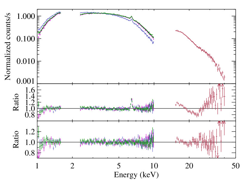
Figure 3.— The time-averaged spectrum for 4U 1538$-$522 before the dip. The continuum model is fdcut. The gap between 1.6 and 2.3 keV is due to uncertainties in the XIS instrumental response in that range. From top to bottom, we plot the spectrum with the best-fitting model, the ratio residuals for a simple absorbed power-law with an fdcut cutoff, and the residuals for the best-fit model, consisting of the absorbed power-law/fdcut continuum with iron K$\alpha$ and K$\beta$ lines and a gauabs feature modeling the CRSF at ${\sim 22}$ keV.

4.2. Time-resolved spectroscopy

Gaps in the lightcurve, caused by the passage of the satellite through the South Atlantic Anomaly, provide convenient points for a time-resolved spectral analysis. We thus divide the observation into nine segments, defined by the SAA gaps. The exception to this is for the fifth and sixth time bins, where the dividing line is placed at the start of the flare rather than during the SAA gap. This ensures that the fifth bin only encompasses the dip, and the sixth, the flare. The time intervals for these spectra are indicated in Figure 1. The HXD/PIN and three XIS spectra for each time bin were initially fit with the same set of models as used for the time-averaged spectrum. The iron K$\beta$ was generally not significantly detected in these spectra, but we did include it in the model (with its energy fixed at $7.056$ keV) in order to obtain upper limits on its intensity. The iron abundance was additionally fixed to the ISM abundance, as it was unconstrained at the high end.

All three continuum models fit the pre-dip and spike spectra well, with $\chi^{2}_{\rm red}\sim 1.0-1.1$. The dip and the final two spectra (spectra 4, 8, and 9 in Table 2), however, show noticeable curvature in their XIS spectra and have much poorer fits, with the dip spectrum having a reduced $\chi^{2}$ of 1.6 for 427 degrees of freedom and spectra 8 and 9 having reduced $\chi^{2}$ of $\sim 1.3$ for 415 and 421 degrees of freedom, respectively. We thus modify the model for these spectra by applying a partial-covering absorption component of the form

$$\mathtt{partcov}(E)=(1-f_{\text{pcf}})*\mathtt{tbnew}_{1}(E)+f_{\text{pcf}}*\mathtt{tbnew}_{2}(E)$$ (8)

This approximates the effect of the source being obscured by a varying absorbing column density. The entire source is absorbed by some base column density $N_{\mathrm{H}}$ (this corresponds to the value of $N_{\mathrm{H}}$ measured by the single tbnew component used in the other spectra), while a region with a higher column density of $N_{\rm H,pcf}$ covers some fraction $f_{\rm pcf}$ of the light from the source. This modification of the model is quite successful, bringing the value of reduced $\chi^{2}$ for the dip spectrum and spectrum 9 down to $\sim 1$ for each continuum model. The lowest-luminosity spectrum, number 8, still has the highest overall $\chi^{2}$ even with the partial-covering model applied, with $\chi^{2}_{\rm red}=1.20$ for 413 degrees of freedom. We attempted to apply the partial-covering model to the remaining spectra, but the covering fraction could not be constrained and the quality of the fit was not improved. In the final two spectra, the addition of the partial-covering model increases the power-law index significantly relative to its value when only a single absorber is used, and the high-energy cutoff parameters are found at values that are more in line with their pre-dip values. While this means comparing the parameters of these spectra to those without the partial-covering model is somewhat risky, it should be noted that our pulse-to-pulse analysis (Section 4.3) finds broadly similar results in terms of $N_{\mathrm{H}}$ and the power-law index.

The fitted parameters for the three continuum models are listed in Table 2. We plot selected parameters against time and unabsorbed flux in Figure 4; as the different continuum models show similar behavior, and in the interests of clarity, we only plot the results from fdcut. For each plotted parameter versus flux, we perform a linear fit and calculate 90% error bars for the slope, as well as computing Pearson’s product-moment correlation coefficient for the data; these results are summarized in Table 3.

Table 2Spectral fits for time-resolved spectroscopy

		1	2	3	4	5	6	7	8	9
highecut
Flux	$\times 10^{-10}$ erg cm-2 s-1	$4.29\pm 0.03$	$5.48\pm 0.05$	$4.59\pm 0.05$	$4.20\pm 0.05$	$4.4\pm 0.2$	$8.7\pm 0.1$	$4.65\pm 0.05$	$2.79^{+0.10}_{-0.09}$	$3.6\pm 0.1$
$N_{\mathrm{H}}$	$\times 10^{22}$ cm-2	$2.22\pm 0.03$	$2.14\pm 0.04$	$2.27\pm 0.05$	$1.98\pm 0.05$	$3.3\pm 0.2$	$2.82\pm 0.08$	$2.16\pm 0.05$	$2.6\pm 0.2$	$3.1\pm 0.2$
$N_{\rm H,pcf}$	$\times 10^{22}$ cm-2	$\cdots$	$\cdots$	$\cdots$	$\cdots$	$17\pm 3$	$\cdots$	$\cdots$	$8^{+4}_{-2}$	$9^{+4}_{-3}$
$f_{\rm pcf}$		$\cdots$	$\cdots$	$\cdots$	$\cdots$	$0.61\pm 0.03$	$\cdots$	$\cdots$	$0.40\pm 0.09$	$0.41^{+0.09}_{-0.08}$
$\Gamma$		$1.16\pm 0.01$	$1.18\pm 0.02$	$1.21\pm 0.02$	$1.20\pm 0.02$	$1.13\pm 0.06$	$0.94\pm 0.03$	$1.11\pm 0.02$	$1.38^{+0.06}_{-0.07}$	$1.38\pm 0.06$
$A$	$\times 10^{-2}$ ph cm-2 s-1	$4.4\pm 0.1$	$5.8\pm 0.2$	$5.1\pm 0.2$	$4.6\pm 0.2$	$4.2^{+0.6}_{-0.5}$	$4.4\pm 0.1$	$4.3\pm 0.2$	$4.1^{+0.6}_{-0.5}$	$5.3^{+0.7}_{-0.6}$
$E_{\mathrm{cut}}$	keV	$24^{+2}_{-4}$	$23^{+3}_{-4}$	$15^{+3}_{-2}$	$22\pm 5$	$21^{+4}_{-5}$	$14.1\pm 0.8$	$18^{+8}_{-5}$	$17^{+6}_{-2}$	$17^{+8}_{-2}$
$E_{\mathrm{fold}}$	keV	$6^{+2}_{-1}$	$7^{+3}_{-2}$	$13^{+2}_{-3}$	$9^{+4}_{-3}$	$8^{+4}_{-2}$	$12\pm 1$	$11^{+4}_{-5}$	$12^{+3}_{-5}$	$12^{+2}_{-6}$
$E_{\mathrm{K}\alpha}$	keV	$6.43\pm 0.01$	$6.43\pm 0.02$	$6.44\pm 0.02$	$6.40\pm 0.02$	$6.41\pm 0.01$	$6.39\pm 0.02$	$6.40\pm 0.02$	$6.42\pm 0.04$	$6.43\pm 0.03$
$I_{\mathrm{K}\alpha}$	$\times 10^{-4}$ ph cm-2 s-1	$3.6^{+0.4}_{-0.3}$	$4.4\pm 0.7$	$3.8\pm 0.6$	$3.3\pm 0.6$	$4.9\pm 0.5$	$8\pm 1$	$3.2\pm 0.6$	$1.2\pm 0.5$	$1.9\pm 0.5$
$I_{\mathrm{K}\beta}$	$\times 10^{-5}$ ph cm-2 s-1	$4\pm 3$	$<8.99$	$<9.39$	$<7.86$	$9\pm 5$	$<15.79$	$<12.43$	$<4.12$	$8\pm 5$
$E_{\mathrm{cyc}}$	keV	$23\pm 1$	$23\pm 1$	$21^{+3}_{-1}$	$22^{+2}_{-1}$	$21.7^{+1.0}_{-0.9}$	$23\pm 1$	$21.3^{+1.0}_{-0.7}$	$21.4^{+0.7}_{-0.6}$	$21.8^{+1.0}_{-0.9}$
$\sigma_{\mathrm{cyc}}$	keV	$3.5\pm 0.6$	$2.5^{+0.7}_{-0.5}$	$3^{+4}_{-2}$	$2.8^{+1.0}_{-0.5}$	$2.5^{+0.7}_{-0.6}$	$>2.12$	$3.2^{+0.8}_{-0.6}$	$0.8^{+1.0}_{-0.6}$	$<3.14$
$\tau_{\mathrm{cyc}}$		$1.1^{+0.1}_{-0.3}$	$0.9^{+0.2}_{-0.3}$	$0.3^{+0.2}_{-0.1}$	$0.9^{+0.2}_{-0.4}$	$0.8^{+0.2}_{-0.4}$	$0.3\pm 0.1$	$0.6^{+0.4}_{-0.3}$	$>0.59$	$0.5^{+90.0}_{-0.2}$
$\chi^{2}_{\rm red}$(dof)		1.02 (434)	1.04 (422)	1.09 (423)	1.10 (422)	1.07 (425)	1.08 (421)	1.05 (425)	1.19 (413)	1.06 (419)
fdcut
Flux	$\times 10^{-10}$ erg cm-2 s-1	$4.28\pm 0.03$	$5.48\pm 0.05$	$4.57^{+0.03}_{-0.05}$	$4.19\pm 0.05$	$4.3\pm 0.2$	$8.7\pm 0.1$	$4.62\pm 0.05$	$2.76^{+0.10}_{-0.09}$	$3.6\pm 0.1$
$N_{\mathrm{H}}$	$\times 10^{22}$ cm-2	$2.21\pm 0.03$	$2.14\pm 0.04$	$2.22^{+0.06}_{-0.07}$	$1.95^{+0.05}_{-0.06}$	$3.2\pm 0.2$	$2.7\pm 0.1$	$2.05^{+0.07}_{-0.08}$	$2.5\pm 0.2$	$3.1\pm 0.2$
$N_{\rm H,pcf}$	$\times 10^{22}$ cm-2	$\cdots$	$\cdots$	$\cdots$	$\cdots$	$16\pm 3$	$\cdots$	$\cdots$	$7^{+4}_{-3}$	$8^{+4}_{-2}$
$f_{\rm pcf}$		$\cdots$	$\cdots$	$\cdots$	$\cdots$	$0.59\pm 0.03$	$\cdots$	$\cdots$	$0.4\pm 0.1$	$0.40\pm 0.09$
$\Gamma$		$1.15\pm 0.02$	$1.17\pm 0.02$	$1.15^{+0.05}_{-0.06}$	$1.17\pm 0.04$	$1.07^{+0.07}_{-0.09}$	$0.85^{+0.06}_{-0.07}$	$0.99^{+0.06}_{-0.07}$	$1.32^{+0.08}_{-0.10}$	$1.34^{+0.07}_{-0.08}$
$A$	$\times 10^{-2}$ ph cm-2 s-1	$4.4\pm 0.1$	$5.7\pm 0.2$	$5.0\pm 0.2$	$4.5\pm 0.2$	$3.9^{+0.6}_{-0.5}$	$4.4\pm 0.1$	$4.4^{+0.4}_{-0.2}$	$3.7^{+0.6}_{-0.5}$	$5.0^{+0.7}_{-0.6}$
$E_{\mathrm{cut}}$	keV	$27\pm 2$	$28\pm 1$	$24^{+6}_{-5}$	$27\pm 3$	$26^{+2}_{-3}$	$22^{+5}_{-4}$	$19^{+5}_{-6}$	$26^{+2}_{-3}$	$28\pm 3$
$E_{\mathrm{fold}}$	keV	$5\pm 1$	$4.0^{+1.0}_{-0.9}$	$7\pm 2$	$6\pm 2$	$5\pm 1$	$7^{+1}_{-2}$	$9\pm 2$	$5\pm 2$	$5\pm 2$
$E_{\mathrm{K}\alpha}$	keV	$6.43\pm 0.01$	$6.43\pm 0.02$	$6.44\pm 0.02$	$6.40\pm 0.02$	$6.41\pm 0.01$	$6.39\pm 0.02$	$6.40\pm 0.02$	$6.42\pm 0.04$	$6.42\pm 0.03$
$I_{\mathrm{K}\alpha}$	$\times 10^{-4}$ ph cm-2 s-1	$3.5\pm 0.3$	$4.4\pm 0.7$	$3.7\pm 0.6$	$3.3\pm 0.6$	$4.9\pm 0.5$	$7\pm 1$	$3.0\pm 0.6$	$1.2^{+0.5}_{-0.4}$	$1.9\pm 0.5$
$I_{\mathrm{K}\beta}$	$\times 10^{-5}$ ph cm-2 s-1	$4\pm 3$	$<8.76$	$<9.03$	$<7.58$	$9\pm 5$	$<14.20$	$<11.33$	$<3.69$	$8\pm 5$
$E_{\mathrm{cyc}}$	keV	$23.2^{+0.7}_{-0.5}$	$23.2^{+0.8}_{-0.6}$	$23^{+2}_{-1}$	$22.6^{+0.8}_{-0.6}$	$22.3^{+0.6}_{-0.5}$	$24^{+2}_{-1}$	$22.1^{+0.8}_{-0.7}$	$22.0^{+0.8}_{-0.6}$	$23\pm 1$
$\sigma_{\mathrm{cyc}}$	keV	$3.4\pm 0.6$	$2.7\pm 0.7$	$3^{+2}_{-1}$	$2.4^{+1.0}_{-0.8}$	$2.4^{+0.8}_{-0.7}$	$3^{+2}_{-1}$	$2\pm 1$	$<2.41$	$3\pm 1$
$\tau_{\mathrm{cyc}}$		$0.9^{+0.2}_{-0.1}$	$0.8\pm 0.1$	$0.4^{+0.2}_{-0.1}$	$0.6^{+0.2}_{-0.1}$	$0.7\pm 0.1$	$0.5^{+0.2}_{-0.1}$	$0.5^{+0.6}_{-0.1}$	$>0.74$	$0.7\pm 0.2$
$\chi^{2}_{\rm red}$(dof)		1.04 (434)	1.06 (422)	1.11 (423)	1.10 (422)	1.09 (425)	1.08 (420)	1.03 (425)	1.20 (413)	1.07 (419)
npex
Flux	$\times 10^{-10}$ erg cm-2 s-1	$4.24\pm 0.03$	$5.51\pm 0.06$	$4.51\pm 0.05$	$4.15\pm 0.05$	$4.7^{+0.4}_{-0.3}$	$8.6\pm 0.1$	$4.55\pm 0.05$	$2.8\pm 0.2$	$4.0^{+0.5}_{-0.3}$
$N_{\mathrm{H}}$	$\times 10^{22}$ cm-2	$2.05\pm 0.05$	$2.14\pm 0.07$	$2.03^{+0.08}_{-0.07}$	$1.76\pm 0.07$	$3.4\pm 0.3$	$2.5\pm 0.1$	$1.83\pm 0.07$	$2.5\pm 0.2$	$3.2\pm 0.3$
$N_{\rm H,pcf}$	$\times 10^{22}$ cm-2	$\cdots$	$\cdots$	$\cdots$	$\cdots$	$19\pm 3$	$\cdots$	$\cdots$	$10\pm 4$	$12^{+4}_{-3}$
$f_{\rm pcf}$		$\cdots$	$\cdots$	$\cdots$	$\cdots$	$0.66^{+0.05}_{-0.06}$	$\cdots$	$\cdots$	$0.4^{+0.1}_{-0.2}$	$0.5\pm 0.1$
$\alpha$		$0.63^{+0.04}_{-0.03}$	$0.79^{+0.06}_{-0.05}$	$0.63^{+0.06}_{-0.05}$	$0.63\pm 0.05$	$0.8\pm 0.2$	$0.36^{+0.07}_{-0.06}$	$0.48^{+0.05}_{-0.04}$	$0.8\pm 0.2$	$1.1\pm 0.3$
$A$	$\times 10^{-2}$ ph cm-2 s-1	$4.3\pm 0.2$	$6.7\pm 0.5$	$4.5^{+0.4}_{-0.3}$	$4.1\pm 0.3$	$6^{+4}_{-2}$	$4.3\pm 0.2$	$3.5^{+0.3}_{-0.2}$	$4^{+2}_{-1}$	$8^{+7}_{-3}$
$B$	$\times 10^{-3}$	$3.2\pm 0.3$	$3.4\pm 0.3$	$2.4\pm 0.4$	$2.5\pm 0.4$	$2.8\pm 0.7$	$4^{+1}_{-2}$	$2.4\pm 0.4$	$2.0^{+0.5}_{-0.4}$	$1.5\pm 0.5$
$k_{\rm B}T$	keV	$4.8\pm 0.1$	$4.7\pm 0.1$	$5.2^{+0.4}_{-0.2}$	$5.1\pm 0.2$	$4.8\pm 0.2$	$5.4^{+1.0}_{-0.4}$	$5.5^{+0.3}_{-0.2}$	$4.7\pm 0.3$	$4.7\pm 0.3$
$E_{\mathrm{K}\alpha}$	keV	$6.43\pm 0.01$	$6.43\pm 0.02$	$6.44\pm 0.02$	$6.40\pm 0.02$	$6.41\pm 0.01$	$6.39\pm 0.02$	$6.40\pm 0.02$	$6.42\pm 0.04$	$6.42\pm 0.03$
$I_{\mathrm{K}\alpha}$	$\times 10^{-4}$ ph cm-2 s-1	$3.6^{+0.4}_{-0.3}$	$4.6\pm 0.7$	$3.8\pm 0.6$	$3.4\pm 0.6$	$5.1\pm 0.6$	$8\pm 1$	$3.1\pm 0.6$	$1.2\pm 0.5$	$2.1\pm 0.6$
$I_{\mathrm{K}\beta}$	$\times 10^{-5}$ ph cm-2 s-1	$4\pm 3$	$<8.80$	$<10.05$	$<8.45$	$10\pm 5$	$<14.67$	$<12.49$	$<4.18$	$10^{+6}_{-5}$
$E_{\mathrm{cyc}}$	keV	$22.6\pm 0.5$	$22.3\pm 0.6$	$23^{+2}_{-1}$	$22.3^{+0.7}_{-0.6}$	$21.9\pm 0.5$	$25^{+4}_{-2}$	$22.3^{+0.8}_{-0.7}$	$21.8^{+0.7}_{-0.6}$	$22.6^{+1.0}_{-0.9}$
$\sigma_{\mathrm{cyc}}$	keV	$2.7\pm 0.5$	$2.4\pm 0.7$	$3^{+2}_{-1}$	$2.3^{+0.8}_{-0.7}$	$2.3\pm 0.7$	$3^{+3}_{-2}$	$2.0\pm 0.9$	$1.0^{+1.0}_{-0.7}$	$3\pm 1$
$\tau_{\mathrm{cyc}}$		$0.66^{+0.09}_{-0.08}$	$0.6\pm 0.1$	$0.4\pm 0.1$	$0.6^{+0.2}_{-0.1}$	$0.6\pm 0.1$	$0.5^{+0.4}_{-0.1}$	$0.5^{+0.3}_{-0.1}$	$>0.69$	$0.6^{+0.2}_{-0.1}$
$\chi^{2}_{\rm red}$(dof)		1.08 (434)	1.00 (422)	1.12 (423)	1.11 (422)	1.08 (425)	1.07 (420)	1.01 (425)	1.20 (413)	1.06 (419)

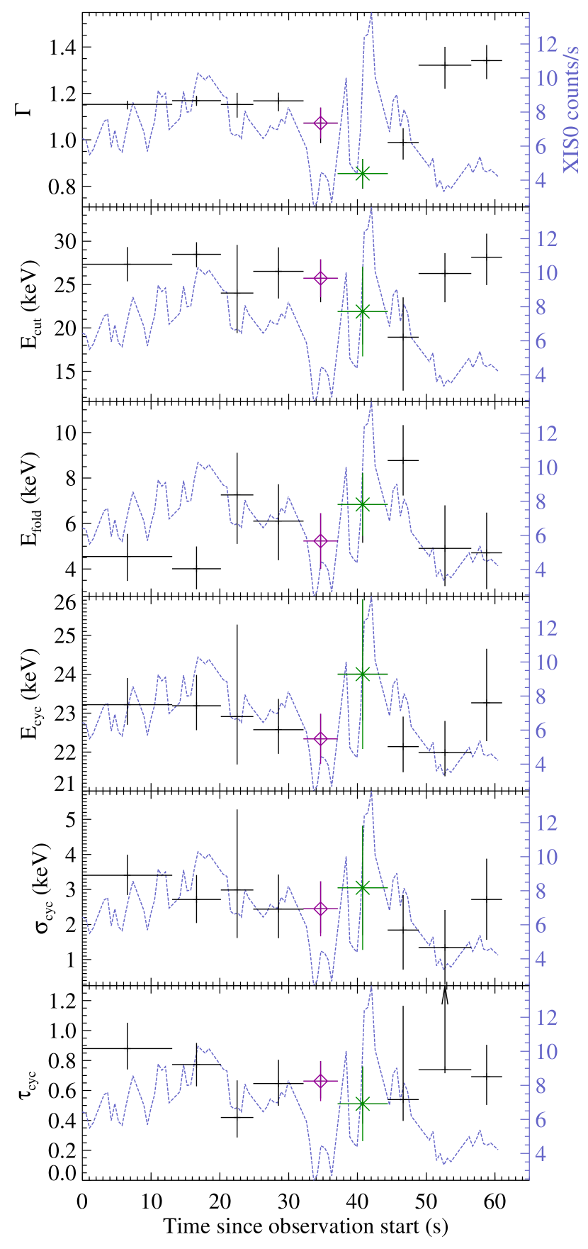
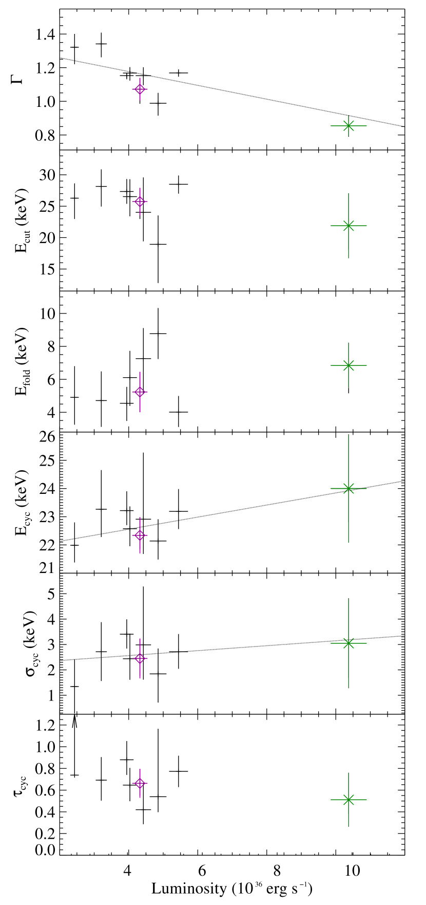
Figure 4.— Selected spectral parameters over the observation, plotted against time (left) and against luminosity (right). For clarity, we only plot results from the fdcut continuum model. The dip spectrum is plotted with a purple diamond, while the flare spectrum uses a green star; all other spectra are plotted in black crosses. When plotted versus time, the XIS0 counting rate is overplotted with a blue dotted line. We overplot the best-fit line for the power-law index, cyclotron line energy, and cyclotron line width vs. luminosity, all of which show significant correlations. The reader should note, however, that the power-law index includes points using differing continuum models, with the dip spectrum as well as the final two spectra adopting a partial-covering absorber and the remaining points using a single-absorber model.

Table 3Linear fits (with 90% error bars) and correlation coefficients for time-resolved spectroscopy

		highecut			fdcut			npex
Parameter	Units	Slope	$r$	$p$-value	Slope	$r$	$p$-value	Slope	$r$	$p$-value
$\Gamma$		$-0.054^{+0.006}_{-0.006}$	$-0.868$	$0.002$	$-0.05^{+0.02}_{-0.02}$	$-0.846$	$0.004$	$\cdots$	$\cdots$	$\cdots$
$E_{\mathrm{cut}}$	keV	$-1.3^{+0.4}_{-0.4}$	$-0.369$	$>0.1$	$-0.5^{+0.9}_{-0.9}$	$-0.465$	$>0.1$	$\cdots$	$\cdots$	$\cdots$
$E_{\mathrm{fold}}$	keV	$0.6^{+0.3}_{-0.3}$	$0.078$	$>0.1$	$0.2^{+0.3}_{-0.3}$	$0.327$	$>0.1$	$\cdots$	$\cdots$	$\cdots$
$\alpha$		$\cdots$	$\cdots$	$\cdots$	$\cdots$	$\cdots$	$\cdots$	$-0.05^{+0.02}_{-0.02}$	$-0.689$	$0.040$
$k_{\rm B}T$	keV	$\cdots$	$\cdots$	$\cdots$	$\cdots$	$\cdots$	$\cdots$	$0.06^{+0.06}_{-0.06}$	$0.599$	$0.088$
$E_{\mathrm{cyc}}$	keV	$0.3^{+0.2}_{-0.2}$	$0.586$	$0.097$	$0.3^{+0.2}_{-0.2}$	$0.690$	$0.040$	$0.4^{+0.2}_{-0.2}$	$0.896$	$0.001$
$\sigma_{\mathrm{cyc}}$	keV	$0.1^{+0.5}_{-0.6}$	$0.094$	$>0.1$	$0.2^{+0.3}_{-0.3}$	$0.407$	$>0.1$	$0.3^{+0.3}_{-0.3}$	$0.624$	$0.072$
$\tau_{\mathrm{cyc}}$		$-0.12^{+0.04}_{-0.04}$	$-0.340$	$>0.1$	$-0.03^{+0.04}_{-0.04}$	$-0.422$	$>0.1$	$-0.02^{+0.03}_{-0.03}$	$-0.534$	$>0.1$

4.3. Pulse-to-pulse analysis

To obtain a more complete picture of the variability of the absorbing column and the iron line, we further divided the observation and extracted spectra for individual pulses. We only examine spectra for full pulses - spectra from fractional pulses are excluded, to avoid contamination by the significant spectral variability within each pulse (see Section 4.4). After excluding fractional pulses, we have a total of 76 spectra. Only XIS spectra are analyzed, as the low exposure for each spectrum precludes the use of PIN data. Each spectrum is fit with a simple model consisting of a single absorbed power-law with an additive Gaussian modeling the iron K$\alpha$ line. This model fits the spectra generally quite well, with an average reduced $\chi^{2}$ of $1.17$. No evidence for partial covering was visible in the residuals, and the partial-covering model used in the previous section for the dip could not be constrained, so the absorption was modeled by a single tbnew component. The cflux model component in XSPEC was used to obtain unabsorbed fluxes for the power-law and the iron line. We plot each parameter with respect to time and luminosity in Figure 5. We also calculated Pearson’s correlation coefficients and performed linear fits on selected parameter versus the 2–10 keV power-law flux; these results are summarized in Table 4. The measured power-law index behaves roughly similar to what was seen in the time-resolved spectroscopy in Section 4.2, despite the use of a partial-covering model in that analysis. However, while the measured absorbing column density in the dip lines up roughly with the partial-covering $N_{\mathrm{H}}$ found in the time-resolved spectroscopy, the slightly-elevated $N_{\mathrm{H}}$ in the final $\sim 10$ pulse-to-pulse spectra do not reach the same levels as the partial-covering model found for the final two time-resolved spectra.

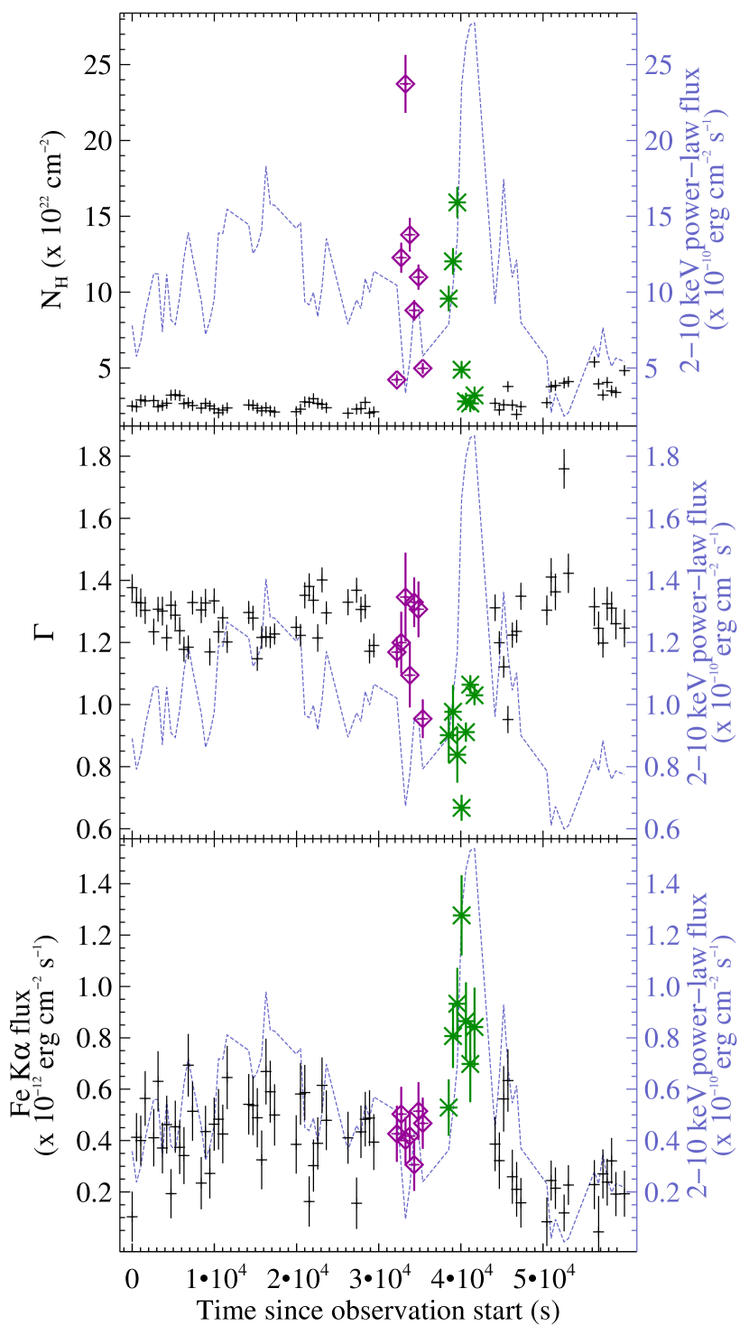
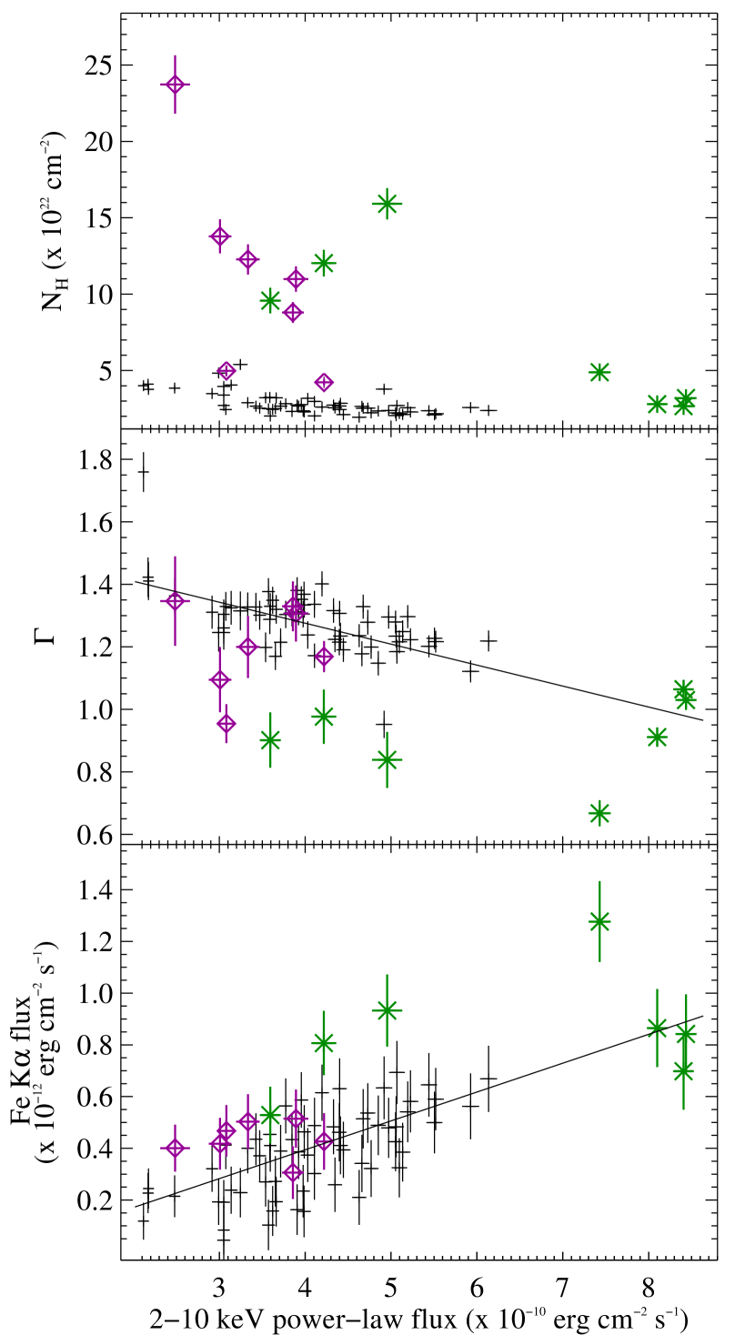
Figure 5.— Parameters versus time (left) and versus flux (right) for the pulse-to-pulse analysis. We plot the first spike in $N_{\mathrm{H}}$ in purple diamonds and the approximate extent of the “flare” state of the source in green stars, with the remainder of the data in black crosses. The unabsorbed power-law flux is rescaled and overplotted as a dashed blue line on the plots versus time. Correlations with luminosity are apparent for the power-law index and the iron K$\alpha$ flux, while the absorbing column density reveals that the dip at around 32 ks in the XIS lightcurve is due to two large spikes in $N_{\mathrm{H}}$.

Table 4Linear fits and correlation coefficients relative to 2–10 keV power-law flux for pulse-to-pulse spectroscopy

Parameter	Units	Slope	$r$	$p$-value
$N_{\mathrm{H}}$	$10^{22}$ cm-2	$-0.07\pm 0.03$	$-0.228$	$0.05$
$\Gamma$		$-0.067\pm 0.008$	$-0.570$	$10^{-7}$
Fe K$\alpha$ flux	$10^{-10}$ erg cm-2 s-1	$0.011\pm 0.002$	$0.707$	$<10^{-8}$

4.4. Phase-resolved spectroscopy

The pulse profile of 4U 1538$-$522 is double-peaked, with a large primary pulse and a significantly smaller secondary pulse (see Figure 5), similar to that found by Robba et al. (2001), Rodes-Roca et al. (2010), and Hemphill et al. (2013). Our phase-resolved analysis was carried out by defining good time intervals for six phase bins, with phase zero defined as the peak of the main pulse. The remaining phase bins thus cover the rising and falling edges of the main pulse, the peak of the secondary pulse, and the low-flux dips on either side of the secondary pulse. This choice of phase binning covers all the major features of the pulse profile without sacrificing signal-to-noise. XIS and PIN spectra were analyzed simultaneously, using the three models described in Section 4.2. The parameters of these three models with 90% error bars are listed in Table 5, and the parameters for the fdcut continuum are plotted in Figure 6. The shape of the continuum, including the cyclotron line, changes considerably between the rising and falling edges of the main pulse. Interestingly, the absorbing column density appears to be significantly dependent on pulse phase (although the magnitude of the effect is relatively small, on the order of 10%). A physical mechanism for this effect is difficult to imagine, and on the whole unlikely - the absorber does not readily show signs of significant ionization, which one would expect if it was close enough to the neutron star to be effected by the star’s rotation. It is likely that the dependence of $N_{\mathrm{H}}$ on pulse phase is in part due to our unphysical modeling of the continuum. This explanation is favored by the fact that the dependence of $N_{\mathrm{H}}$ on pulse phase varies with the choice of continuum model - under highecut, $N_{\mathrm{H}}$ is roughly constant in all bins save the peak of the main pulse, where it drops suddenly, while in fdcut and npex the $N_{\mathrm{H}}$ follows a more “sawtooth” pattern, dropping sharply at the main pulse but rising slowly afterwards. Meanwhile, the CRSF parameters and iron line intensity all show strong dependence on phase, without any strong dependence on continuum model.

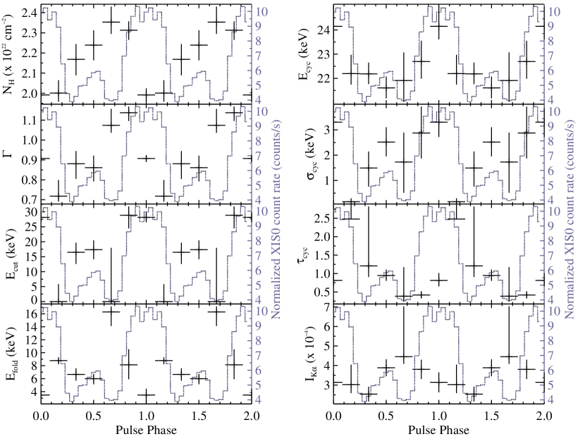
Figure 6.— Selected parameters for the phase-resolved fits. The spectral parameters for the fdcut continuum are plotted as crosses, while the pulse profile in the 2-10 keV band is overplotted with a blue dotted line. For clarity, the pulse profile is repeated. The vertical axis on the right of each plot indicates the normalized XIS count rate for the pulse profile. The apparent dependence of $N_{\mathrm{H}}$ on pulse phase is dependent on the choice of continuum model and likely reflects the fact that our empirical continuum models do not perfectly model the underlying continuum, rather than representing a true modulation of the obscuring column density.

Table 5Spectral fits for phase-resolved spectroscopy

		Phase bin
		1	2	3	4	5	6
highecut
Flux	$\times 10^{-10}$ erg cm-2 s-1	$6.32\pm 0.04$	$4.59\pm 0.04$	$2.98\pm 0.03$	$3.67\pm 0.03$	$2.60\pm 0.03$	$5.47\pm 0.04$
$N_{\mathrm{H}}$	$\times 10^{22}$ cm-2	$2.00\pm 0.03$	$2.34\pm 0.04$	$2.30\pm 0.05$	$2.35\pm 0.05$	$2.53\pm 0.05$	$2.35\pm 0.04$
$\Gamma$		$0.91\pm 0.01$	$1.13\pm 0.02$	$1.02\pm 0.02$	$0.98\pm 0.02$	$1.28\pm 0.02$	$1.18\pm 0.02$
$A$	$\times 10^{-2}$ ph cm-2 s-1	$4.2\pm 0.1$	$4.4\pm 0.1$	$2.37\pm 0.09$	$2.72\pm 0.09$	$3.2\pm 0.1$	$5.7^{+0.2}_{-0.1}$
$E_{\mathrm{cut}}$	keV	$23\pm 3$	$12.5^{+0.6}_{-0.7}$	$14^{+4}_{-1}$	$23^{+4}_{-8}$	$14^{+9}_{-2}$	$18^{+8}_{-4}$
$E_{\mathrm{fold}}$	keV	$6^{+1}_{-2}$	$10.1\pm 0.7$	$9.1^{+0.9}_{-2.0}$	$4^{+4}_{-1}$	$21^{+5}_{-10}$	$17^{+5}_{-7}$
$E_{\mathrm{K}\alpha}$	keV	$6.41\pm 0.02$	$6.41\pm 0.02$	$6.42\pm 0.02$	$6.43\pm 0.01$	$6.415^{+0.009}_{-0.008}$	$6.42\pm 0.01$
$I_{\mathrm{K}\alpha}$	$\times 10^{-4}$ ph cm-2 s-1	$3.2\pm 0.5$	$3.3\pm 0.4$	$2.6\pm 0.4$	$4.0\pm 0.4$	$4.6\pm 0.4$	$3.9\pm 0.5$
$I_{\mathrm{K}\beta}$	$\times 10^{-5}$ ph cm-2 s-1	$<8.00$	$<7.00$	$5\pm 4$	$5\pm 4$	$6\pm 3$	$<7.00$
$E_{\mathrm{cyc}}$	keV	$23.4^{+1.0}_{-0.8}$	$21.9\pm 0.6$	$21.9\pm 0.5$	$22\pm 2$	$21\pm 1$	$21.4^{+0.7}_{-0.6}$
$\sigma_{\mathrm{cyc}}$	keV	$3.0^{+0.6}_{-0.3}$	$0.33$ (fixed)	$2\pm 1$	$3.5^{+1.0}_{-0.4}$	$2.82$ (fixed)	$3.0^{+0.6}_{-2.0}$
$\tau_{\mathrm{cyc}}$		$0.9\pm 0.2$	$2^{+2}_{-1}$	$1.0^{+2.0}_{-0.3}$	$1.7^{+0.2}_{-0.9}$	$0.3^{+0.4}_{-0.1}$	$0.4^{+0.3}_{-0.2}$
$\chi^{2}_{\rm red}$(dof)		1.14 (432)	1.36 (423)	1.28 (417)	1.08 (423)	1.14 (427)	1.17 (438)
fdcut
Flux	$\times 10^{-10}$ erg cm-2 s-1	$6.32\pm 0.04$	$4.49^{+0.04}_{-0.03}$	$2.94\pm 0.03$	$3.63\pm 0.04$	$2.58\pm 0.03$	$5.46\pm 0.04$
$N_{\mathrm{H}}$	$\times 10^{22}$ cm-2	$1.99\pm 0.03$	$2.00^{+0.06}_{-0.04}$	$2.17\pm 0.08$	$2.24^{+0.07}_{-0.08}$	$2.35^{+0.08}_{-0.06}$	$2.31^{+0.04}_{-0.05}$
$\Gamma$		$0.91^{+0.01}_{-0.02}$	$0.72^{+0.08}_{-0.03}$	$0.88^{+0.06}_{-0.08}$	$0.86^{+0.06}_{-0.07}$	$1.07^{+0.08}_{-0.04}$	$1.14^{+0.03}_{-0.04}$
$A$	$\times 10^{-2}$ ph cm-2 s-1	$4.2\pm 0.1$	$6.4^{+0.2}_{-1.0}$	$2.26^{+0.10}_{-0.09}$	$2.56^{+0.10}_{-0.09}$	$5.4^{+0.3}_{-2.0}$	$5.7\pm 0.2$
$E_{\mathrm{cut}}$	keV	$28\pm 2$	$<6.01$	$16^{+3}_{-4}$	$17\pm 3$	$<20.01$	$29^{+3}_{-4}$
$E_{\mathrm{fold}}$	keV	$3\pm 1$	$8.8^{+0.2}_{-0.5}$	$6.6^{+1.0}_{-0.9}$	$6.0^{+0.7}_{-0.9}$	$16.3^{+0.9}_{-2.0}$	$8\pm 2$
$E_{\mathrm{K}\alpha}$	keV	$6.41\pm 0.02$	$6.42\pm 0.02$	$6.42\pm 0.02$	$6.43\pm 0.01$	$6.415\pm 0.009$	$6.42^{+0.02}_{-0.01}$
$I_{\mathrm{K}\alpha}$	$\times 10^{-4}$ ph cm-2 s-1	$3.1\pm 0.5$	$3.0^{+1.0}_{-0.4}$	$2.5\pm 0.4$	$3.9\pm 0.4$	$4.5^{+3.0}_{-0.4}$	$3.8\pm 0.5$
$I_{\mathrm{K}\beta}$	$\times 10^{-5}$ ph cm-2 s-1	$<8.00$	$<6.00$	$5\pm 4$	$<8.00$	$6^{+5}_{-3}$	$<7.00$
$E_{\mathrm{cyc}}$	keV	$24.1^{+0.8}_{-0.5}$	$22.2^{+0.8}_{-0.5}$	$22.2^{+0.5}_{-0.4}$	$21.6^{+0.5}_{-0.4}$	$21.9^{+1.0}_{-0.9}$	$22.7^{+0.9}_{-0.7}$
$\sigma_{\mathrm{cyc}}$	keV	$3.3\pm 0.6$	$0.16$ (fixed)	$1.5\pm 0.7$	$2.5\pm 0.6$	$2\pm 1$	$3\pm 1$
$\tau_{\mathrm{cyc}}$		$0.8\pm 0.2$	$>7.69$	$1.2^{+2.0}_{-0.3}$	$0.9^{+0.2}_{-0.1}$	$0.4^{+0.8}_{-0.1}$	$0.42^{+0.10}_{-0.08}$
$\chi^{2}_{\rm red}$(dof)		1.15 (432)	1.05 (423)	1.26 (417)	1.05 (423)	1.10 (426)	1.18 (438)
npex
Flux	$\times 10^{-10}$ erg cm-2 s-1	$6.31^{+0.05}_{-0.04}$	$4.42\pm 0.04$	$2.90\pm 0.03$	$3.60\pm 0.04$	$2.54\pm 0.03$	$5.40\pm 0.04$
$N_{\mathrm{H}}$	$\times 10^{22}$ cm-2	$1.91\pm 0.05$	$1.83\pm 0.05$	$1.95\pm 0.08$	$2.05\pm 0.08$	$2.15^{+0.07}_{-0.06}$	$2.13\pm 0.05$
$\alpha$		$0.50\pm 0.04$	$0.32\pm 0.03$	$0.33\pm 0.06$	$0.33\pm 0.06$	$0.64\pm 0.04$	$0.66\pm 0.03$
$A$	$\times 10^{-2}$ ph cm-2 s-1	$4.5^{+0.3}_{-0.2}$	$3.1^{+0.2}_{-0.1}$	$1.9\pm 0.2$	$2.4\pm 0.2$	$2.4^{+0.2}_{-0.1}$	$5.1\pm 0.3$
$B$	$\times 10^{-3}$	$5.2\pm 0.3$	$2.8\pm 0.6$	$4.9\pm 0.8$	$6.7\pm 0.9$	$1.1^{+0.4}_{-0.3}$	$1.8\pm 0.2$
$k_{\rm B}T$	keV	$5.0\pm 0.1$	$4.8\pm 0.2$	$4.6\pm 0.2$	$4.3\pm 0.2$	$6.1^{+0.6}_{-0.4}$	$5.9\pm 0.2$
$E_{\mathrm{K}\alpha}$	keV	$6.41\pm 0.02$	$6.42\pm 0.02$	$6.42\pm 0.02$	$6.43\pm 0.01$	$6.415^{+0.009}_{-0.008}$	$6.42\pm 0.01$
$I_{\mathrm{K}\alpha}$	$\times 10^{-4}$ ph cm-2 s-1	$3.2\pm 0.5$	$3.2\pm 0.5$	$2.6\pm 0.4$	$3.9\pm 0.5$	$4.6\pm 0.4$	$4.0\pm 0.5$
$I_{\mathrm{K}\beta}$	$\times 10^{-5}$ ph cm-2 s-1	$<7.00$	$<8.00$	$5\pm 4$	$5\pm 4$	$7\pm 3$	$<8.00$
$E_{\mathrm{cyc}}$	keV	$23.9^{+0.5}_{-0.4}$	$22.1^{+0.5}_{-0.4}$	$22.3^{+0.5}_{-0.4}$	$21.7^{+0.5}_{-0.4}$	$21.9^{+1.0}_{-0.8}$	$22.4\pm 0.6$
$\sigma_{\mathrm{cyc}}$	keV	$2.1\pm 0.5$	$0.33$ (fixed)	$1.5^{+0.6}_{-0.7}$	$2.4\pm 0.5$	$2\pm 1$	$3.4\pm 0.7$
$\tau_{\mathrm{cyc}}$		$0.48^{+0.09}_{-0.08}$	$4^{+4}_{-2}$	$1.2^{+2.0}_{-0.3}$	$0.9^{+0.2}_{-0.1}$	$0.4^{+0.2}_{-0.1}$	$0.46\pm 0.06$
$\chi^{2}_{\rm red}$(dof)		1.24 (432)	1.05 (424)	1.27 (417)	1.07 (423)	1.07 (426)	1.15 (438)

5. Discussion

Our observation of 4U 1538$-$522 reveals intriguing results in three broad areas. The line-of-sight column density increases drastically $\sim 32$ ks into the observation, and this is followed quickly by an X-ray flare. The increase in $N_{\mathrm{H}}$ is not associated with any additional changes in the continuum, implying that the source of the $N_{\mathrm{H}}$ increase is relatively distant from the neutron star accretion column, while the flare is associated with a significant increase in spectral hardness. The iron K$\alpha$ intensity varies with luminosity and with pulse phase, giving an indication of the illuminated iron’s overall distance from the neutron star. And the cyclotron line energy has a weak dependence on the source’s luminosity, revealed by the high-luminosity flare.

5.1. Variability of Absorption and Continuum

As can be seen in Figures 4 and 5, the column density and continuum parameters during the pre-dip portion of the observation stay relatively constant, with $N_{\mathrm{H}}$ at an average value of $2.16\times 10^{22}$ cm^-2 in the pulse-to-pulse dataset. However, with the onset of the dip $\sim 32$ ks into the observation, the measured column density increases drastically, first spiking to $\left(24\pm 2\right)\times 10^{22}$ cm^-2, quickly falling back to pre-dip levels, and then, immediately before the peak of the flare, rising again to $\left(16\pm 2\right)\times 10^{22}$ cm^-2. We note that the partial-covering model in the time-resolved spectrum of the dip reaches similar column densities ($\left(19\pm 3\right)\times 10^{22}$ cm^-2) to the pulse-to-pulse results, suggesting that the necessity of the partial coverer may be due to the averaging of spectra with varying $N_{\mathrm{H}}$, rather than a spatial partial coverer. The spikes in $N_{\mathrm{H}}$ suggest that the dip is caused by some overdense region of the accreted stellar wind passing through the line of sight. The duration of the increases in $N_{\mathrm{H}}$ along with the fact that the other continuum parameters do not change significantly during the dip indicates that the material producing the additional absorption must be relatively far from the star, as otherwise the material would be accreted onto the star in a relatively short time, changing the continuum emission and increasing the flux.

The continuum parameters (power-law index and cutoff and folding energies) are generally flat for the first half of the observation, remaining this way until a few pulsations before the peak of the flare, when the power-law index drops (in both the time-resolved spectra and the pulse-to-pulse spectra) by a factor of approximately 1/3. While the peak of the flare is clearly visible in the lightcurve, the point where the power-law index drops is a better approximation of the “true” starting point of the flare, with the beginning stages of the flare being obscured by the second spike in $N_{\mathrm{H}}$. The unabsorbed flux is indeed climbing during the three pulses before the peak of the flare, as can be seen in the overplotted lightcurve in Figure 5. While the cutoff and folding energies do change slightly with the onset of the flare, they are poorly constrained compared to the power-law index, so it is difficult to see the effect of the flare in these parameters. The cutoff energy does appear to drop during the flare and in the first post-flare spectrum, before rising back to its pre-flare levels, while the even more poorly constrained folding energy (and $kT$ in the npex model) rises during the flare. However, these effects are statistically very weak.

The source after the flare is less luminous, in terms of unabsorbed flux, than it was before the flare. In the pulse-to-pulse spectra, the power-law index additionally shows an overall negative correlation with luminosity, with a slope of $-0.067\pm 0.008$ per $10^{-10}$ erg cm^-2 s^-1. Pearson’s coefficient for this is $-0.58$, which for 76 points corresponds to a two-tailed p-value of less than $10^{-5}$. This trend is preserved even if we exclude the dip and the spike from the calculation, although the slope drops slightly to $-0.058\pm 0.011$ per $10^{-10}$ erg cm^-2 s^-1. The time-resolved spectra show a similar correlation, with a slope of $-0.05\pm 0.02$ per $10^{-10}$ erg cm^-2 s^-1. This lends some credence to the partial-covering model used in the final two spectra of the time-resolved analysis — without the partial-covering model, the power-law index in the time-resolved spectra does not show a significant correlation with flux.

The continuum parameters generally show variability with phase, with the different continuum models displaying similar behavior. The power-law index, cutoff energy, folding energy, and npex’s $kT$ all show a peak somewhere around the rising edge of the main pulse, and roughly trend downward until the secondary pulse. The spectral shape of the rising and falling edges of the main pulse are distinctly different. Our continuum results are similar to those found using other satellites by, e.g., Clark et al. (1990), Coburn (2001), and Robba et al. (2001).

One potential area of concern is that the dip or flare represent some anomalous behavior of the source, and including those data with the non-flaring, less-obscured data may skew our results with regards any observed correlations. However, the observed trends all persist even if we remove the dip and the flare from the sample, indicating that the trends are somewhat fundamental to the longer-term behavior of the source. The plot of iron line flux vs. power-law flux with the dip and flare excluded has the same slope of $(1.1\pm 0.2)\times 10^{-3}$ as found before, while the power-law index has a slightly smaller slope, $-0.058\pm 0.011$, but still consistent with the earlier result. Removing the dip and flare obviously produces larger changes in the behavior of $N_{\mathrm{H}}$, but the overall appearance of the parameter when plotted against the power-law flux is somewhat unchanged - there is an overall negative trend, as one would expect, with increased scatter in the measured $N_{\mathrm{H}}$ as the luminosity decreases. This increased scatter in $N_{\mathrm{H}}$ can be investigated by looking at the (lack of a) correlation between $N_{\mathrm{H}}$ and the power-law index: periods of increased $N_{\mathrm{H}}$ do not tend to be immediately related to changes in spectral hardness.

5.1.1 Connection between absorption event and flare

The presence of the flare in the lightcurve is evidence of some degree of clumpiness or structure in the stellar wind of QV Nor (although simulations have shown that highly variable accretion can occur even in the presence of a relatively smooth stellar wind; see, e.g., Manousakis et al., 2014). The increased $N_{\mathrm{H}}$ seen before the flare is a possible source of the material accreted during the flare. However, if this is the case, the total amount of matter in the clump should reflect the observed luminosity during the flare. The $N_{\mathrm{H}}$ variability has a two-peak structure, with one large peak reaching $\sim 25\times 10^{22}$ cm^-2 several ks before the flare and a smaller peak immediately before the flare that reaches $\sim 15\times 10^{22}$ cm^-2. By following a method similar to that applied to Vela X–1 by Martínez-Núñez et al. (2014), we can estimate the size and, more importantly, the mass of the overdensity in the stellar wind. We will first assume that the spikes in $N_{\mathrm{H}}$ are caused by overdensities that move with the stellar wind. Using the orbital solution from Mukherjee et al. (2006), the Suzaku observation was carried out at an orbital phase of $\sim 0.3$, and so we will additionally assume that the wind is moving roughly perpendicular to the line of sight.

In general, the wind velocity at a given distance will depend on the terminal wind velocity $v_{\infty}$ via

$$v_{\rm wind}(r)=v_{\infty}\left(1-\frac{R_{\rm opt}}{r}\right)^{\beta}$$ (9)

The terminal wind velocity can in turn be estimated from the escape velocity for QV Nor via the correlation plot in Abbott (1982). From Clark et al. (1994), we have

$$v_{\rm esc} = \left[2GM_{\rm opt}\left(1-L_{\rm opt}/L_{\rm Edd}\right)/R_{\rm opt}\right]^{1/2}$$ (10)

$$\approx 600\>\mathrm{km}\,\mathrm{s}^{-1}$$ (11)

In these equations, $M_{\rm opt}\sim 15$ $M_{\odot}$, $R_{\rm opt}\sim 16$ $R_{\odot}$, $\beta\sim 0.9$, $L_{\rm opt}=1.6\times 10^{5}$ $L_{\odot}$, and $L_{\rm Edd}\sim 5\times 10^{5}$ $L_{\odot}$ are the mass, radius, Roche lobe filling factor, luminosity, and Eddington luminosity of QV Nor (Reynolds et al., 1992; Rawls et al., 2011). From Abbott (1982), $v_{\infty}\sim 1300-1800$ km s^-1. A range of values have been reported for the mass and radius of QV Nor, with Reynolds et al. (1992) finding $M_{\rm opt}=19.9\pm 3.4$ $M_{\odot}$ and Rawls et al. (2011) finding $20.72\pm 2.27$ $M_{\odot}$ and $14.13\pm 2.78$ $M_{\odot}$ for the elliptical and circular orbital solutions, respectively, but these differences do not have large effects on our results here due to the imprecision in estimating the terminal wind velocity.

At an inclination of $\sim 70$ degrees (Rawls et al., 2011), the semimajor axis of the binary system is $\sim 1.7\times 10^{12}$ cm, and at this distance the wind velocity is $\sim 7\times 10^{7}$ cm s^-1. The length scales of the overdensities can thus be estimated from their time of passage through the line of sight from $v_{\rm wind}t_{\rm pass}\sim 2\times 10^{11}$ cm for the large spike and $\sim 1\times 10^{11}$ cm for the smaller spike. The average excess column densities over the extent of each spike in $N_{\mathrm{H}}$ are $9.1\times 10^{22}$ cm^-2 for the earlier, larger spike and $9.2\times 10^{22}$ cm^-2 for the second, smaller spike. The similarity in average column density is due to the shorter duration of the second spike ($\sim 3$ pulse periods) compared to the first spike ($\sim 7$ pulse periods). Given the estimated length scales, these imply number densities of $\sim 4\times 10^{11}$ H atoms cm^-3 and $\sim 8\times 10^{11}$ H atoms cm^-3, respectively, and thus masses of $\sim 10^{22}$ g and $2\times 10^{21}$ g. These represent a factor of $\sim$ 50–100 overdensity compared to the $\sim 5\times 10^{9}$ cm^-3 in the wind at the neutron star’s distance from QV Nor (Clark et al., 1994).

The X-ray flare persists for $\sim 7$ pulse periods, if we define the “flare” state as when the source is spectrally harder (the green stars in Figure 5). If the material from the larger spike in $N_{\mathrm{H}}$ was fully accreted by the neutron star, the mass accretion rate would be $\sim 10^{18}$ g s^-1. If $\eta$, the efficiency of converting gravitational energy to X-rays, is $\sim 10$%, the X-ray luminosity would be

$$L_{\rm flare} = \eta\frac{GM_{\rm X}\dot{M}}{R_{\rm X}}$$ (12)

$$\approx 3\times 10^{37}\>\mathrm{erg}\,\mathrm{s}^{-1}$$ (13)

The 5–100 keV X-ray luminosity measured during the flare is somewhat lower than this, with a peak luminosity of $1\times 10^{37}$ erg s^-1. However, the structure of the $N_{\mathrm{H}}$ variability, with the second peak during the flare and increased $N_{\mathrm{H}}$ post-flare, indicates that it is unlikely that the entirety of the overdense region was accreted onto the neutron star during the flare. Nonetheless, it is clear that the increased $N_{\mathrm{H}}$ seen during the dip represents enough material to support the observed flaring.

5.2. Iron line

In both the time-resolved and the pulse-to-pulse spectra, the Fe K$\alpha$ line has a significant positive correlation with flux. The points from the dip are slight outliers, remaining at roughly the same level as before the dip during the first spike in $N_{\mathrm{H}}$, and rising with the flare during the second, smaller peak in $N_{\mathrm{H}}$. The iron line’s insensitivity to the dip is not surprising, considering that the flux above $\sim 5$ keV is largely unaffected by the large increase in $N_{\mathrm{H}}$ that produces the dip. In the pulse-to-pulse spectra, Pearson’s correlation coefficient is 0.701, which indicates a very strong correlation. A linear fit to the pulse-to-pulse data returns a slope of $\left(1.1\pm 0.2\right)\times 10^{-2}$. The strong correlation between power-law flux and iron line flux implies that the iron must be fairly close to the neutron star (i.e. with a relatively small light travel time between the neutron star’s continuum emission and the surrounding iron). The cross-correlation of the pulse-to-pulse iron line fluxes and power-law fluxes peaks at a lag of zero, which at our time resolution places an upper limit on this light travel time of $525.59$ s, or a distance of $\sim 1.5\times 10^{13}$ cm. Meanwhile, phase-resolved spectroscopy shows the iron line varying with phase, following the general shape of the pulse profile, but with a significant phase lag of $\sim 0.67$, or $\sim 350$ s. If we assume that the iron emission peaks due to the light from the peak of the pulse, this would imply a distance of $\sim 10^{13}$ cm, or $\sim 1$ AU. Work by Rodes-Roca et al. (2010) using XMM-Newton found variability of the iron line with phase, but they only report the iron line equivalent width, and with the complex continuum that they use, a direct comparison is difficult. Robba et al. (2001) divided the BeppoSAX spectrum of 4U 1538$-$522 into four phase bins, and while they could not constrain the intensity of the iron line especially well, their results are broadly in line with ours, with the brightest iron K$\alpha$ offset from the main pulse.

Our constraints on the iron K$\beta$ line provide some limited additional insight in this area, as the ratio of the K$\beta$ intensity to the K$\alpha$ intensity is a probe of the level of ionization of the iron. While we typically only find upper limits on the K$\beta$ intensity, the values we do find are consistent with neutral iron, with the K$\beta$ to K$\alpha$ intensity ratio sitting around the expected $13.5$% (Palmeri et al., 2005). This is again consistent with the distance found via the cross-correlation and the phase-resolved spectroscopy - if the iron is indeed at an average distance of $\sim 1$ AU, we should not expect to see any strong signature of ionization.

5.3. Cyclotron scattering feature

The behavior of the cyclotron line over the course of the observation is our final feature of interest. This pseudo-absorption feature is produced when photons are scattered out of the line of sight by electrons in the accretion column above the neutron star’s magnetic poles. In the $\sim 10^{12}$ G magnetic field of the neutron star, the cyclotron motion of the electrons is quantized into Landau levels, and thus photons see an elevated scattering cross-section when they have sufficient energy to send an electron into the next level. This scattering results in a net reduction in line-of-sight photons at around the CRSF energy. The “12-B-12” rule gives an approximate relation between the observed CRSF energy and the magnetic field strength in the scattering region:

$$E_{\mathrm{cyc}}=\frac{11.57\,\mathrm{keV}}{1+z}\times B_{12}$$ (14)

where $B_{12}$ is the magnetic field in units of $10^{12}$ G and $z\sim 0.15$ is the gravitational redshift in the scattering region. 4U 1538$-$522’s CRSF energy of $\sim 23$ keV implies a magnetic field strength of $\sim 2.2-2.3\times 10^{12}$ G, assuming a radius of $10$ km and a mass of either $0.87\pm 0.07$ $M_{\odot}$ or $1.104\pm 0.177$ $M_{\odot}$, per Rawls et al. (2011). Our measured cyclotron line energy is moderately higher than many previously measured values, with Clark et al. (1990), Robba et al. (2001), and Coburn (2001) all finding CRSF energies around $\sim 20-21$ keV, while our CRSF energy is closer to $\sim 23$ keV. The results of Rodes-Roca et al. (2009) and Hemphill et al. (2013) are closer in line with ours. While the possibility of a long-term change over time in the cyclotron line energy is intriguing, a proper comparison with past work would need to take much more careful account of the differing instruments and models (both for the continuum and the CRSF) used by different authors, as these can have not insignificant effects on the measured line energy (see, e.g. Müller et al., 2013).

The cyclotron line energy reaches a peak value of $\sim 24$ keV during the flare, and there is a positive correlation between the CRSF energy and luminosity. Our linear fits to the data find a slope of $0.3\pm 0.2$ keV per $10^{-10}$ erg cm^-2 s^-1 in the fdcut and highecut models and $0.4\pm 0.2$ keV per $10^{-10}$ erg cm^-2 s^-1 when using npex. This is somewhat dependent on the inclusion of the point from the flare: if the flare is excluded, the slope for the fdcut continuum changes to $0.3\pm 0.3$, which, while just barely consistent with zero, is still notably inconsistent with a negative slope.

Current theory regarding the cyclotron line, according to Becker et al. (2012), finds that the CRSF energy should exhibit different behavior with respect to source luminosity depending on the luminosity regime of the source. When the accretion column is locally super-Eddington ($L>L_{\mathrm{crit}}$ in Becker et al.), increases in luminosity should push the line-emitting region upward, towards lower magnetic fields, while below this critical luminosity, the opposite should occur. At still lower luminosities, the line-producing region should be relatively close to the neutron star surface, and is not expected to change drastically with changes in luminosity.

After computing the luminosity of 4U 1538$-$522 for each time-resolved spectrum from the 5–100 keV flux assuming a distance of $6.4$ kpc (Reynolds et al., 1992), we can compare our results with the predictions of Becker et al. (2012). $L_{\rm crit}$ is given by equation 32 in Becker et al. (2012):

$$L_{\rm crit} = 1.49\times 10^{37}{\rm erg\,s}^{-1}\left(\frac{\Lambda}{0.1}\right)^{-7/5}w^{-28/15}$$ (15)

$$\times\left(\frac{M}{1.4{\rm\,M}_{\odot}}\right)^{29/30}\left(\frac{R}{10{\rm\,km}}\right)^{1/10}\left(\frac{B_{\rm surf}}{10^{12}{\rm\,G}}\right)^{16/15}$$

Here, $M$, $R$, and $B$ are, respectively, the mass, radius, and surface magnetic field strength of the neutron star, $w=1$ characterizes the shape of the photon spectrum inside the column (where there is assumed to be a mean photon energy of $\bar{E}=wkT_{\rm eff}$), and $\Lambda$ characterizes the mode of accretion. Becker et al. only consider the case of $\Lambda=0.1$, which approximates disk accretion. With this value for $\Lambda$, 4U 1538$-$522 is sub-critical, with the $L_{\rm coul}$ cut-off of Becker et al. (2012) sitting approximately between the highest non-flaring luminosity and the flare, and the Becker et al. (2012) predictions hold. However, 4U 1538$-$522 is believed to be a wind-accreting source, rather than a disk accretor, and thus we should choose $\Lambda=1$ in our calculations. This presents us with an interesting result: the value for $L_{\rm crit}$ drops considerably, in fact falling below the $L_{\rm coul}$ cut-off. It is uncertain as to what the theory predicts in this regime. This is the same as was found by Fürst et al. (2014) for Vela X$-$1, another wind-accreting HMXB of similar luminosity and with a CRSF of comparable energy ($\sim 25$ keV).

The problematic parameter here is $\Lambda$, which is difficult to determine precisely. The $w$ parameter is unlikely to diverge much from $w=1$, as the spectrum inside the accretion column is dominated by bremsstrahlung emission (Becker & Wolff, 2007), and our results do not change significantly when $w$ is varied around its assumed value of 1. The $\Lambda$ parameter, on the other hand, is tied to the Alfvén radius $R_{\rm A}$, as $R_{\rm A}$ in the disk of a disk-accreting source will be smaller than $R_{\rm A}$ for a wind-accretor experiencing a similar $\dot{M}$. Fürst et al. (2014) suggest that a very narrow accretion column could cause a breakdown of the theory in this case, and as the accretion column radius is tied to the Alfvén radius, differing values for $\Lambda$ could have an effect here. However, it is also possible that the assumption of $\Lambda=1$ is not precisely correct for 4U 1538$-$522; that is, the mode of accretion is not purely spherical. If the overdensity that produces the flare possesses significant angular momentum relative to the average angular momentum in the stellar wind, a transient disk may form during the flare and change the value of $\Lambda$ from its value during the non-flaring state of the source.

To examine this, we fit the predicted $E_{\rm cyc}$ from Becker et al. (2012) to our cyclotron line energy measurements. The free parameters were $\Lambda$ and the surface cyclotron line energy $E_{\rm surf}$, although we limited $E_{\rm surf}$ to be greater than our largest measured $E_{\rm cyc}$ (i.e., we assumed that the magnetic field our observation samples is weaker than the magnetic field at the surface). The mass of the neutron star was set to $1.104$$M_{\odot}$ (although using the lower-mass estimate from Rawls et al. (2011) did not change our results significantly), and the radius was assumed to be $10$ km. As in Becker et al. (2012), we assume a dipole magnetic field. The theoretical $E_{\rm cyc}$ is thus dependent on the altitude $h$ above the neutron star’s surface:

$$\frac{E_{\rm cyc}}{E_{\rm surf}}=\left(\frac{R+h}{R}\right)^{-3}$$ (16)

where $h$ is given by

$$h_{\rm s} = 2.28\times 10^{3}{\rm\,cm}\left(\frac{\xi}{0.01}\right)\left(\frac{M}{1.4{\rm\,M}_{\odot}}\right)^{-1}$$ (17)

$$\times\left(\frac{R}{10{\rm\,km}}\right)\left(\frac{L_{\rm X}}{10^{37}{\rm\,erg\,s}^{-1}}\right)$$

for a supercritical source and by

$$h_{\rm c} = 1.48\times 10^{5}{\rm\,cm}\left(\frac{\Lambda}{0.1}\right)^{-1}\left(\frac{\tau}{20}\right)\left(\frac{M}{1.4{\rm\,M}_{\odot}}\right)^{19/14}$$ (18)

$$\times\left(\frac{R}{10{\rm\,km}}\right)^{1/14}\left(\frac{B_{\rm surf}}{10^{12}{\rm\,G}}\right)^{-4/7}\left(\frac{L_{\rm X}}{10^{37}{\rm\,erg\,s}^{-1}}\right)^{-5/7}$$

for a subcritical source. This defines a piecewise function for $E_{\rm cyc}$, which we fit to our results. For the fdcut continuum model, the fitted values were $\Lambda=0.348^{+0.002}_{-0.058}$ and $E_{\rm surf}=24.68^{+0.36}_{-0.03}$ keV. This best-fit result is plotted over the measured values for $E_{\rm cyc}$ in Figure 7. We additionally fit the predicted cyclotron line energy fixed $\Lambda=1.0$ and $\Lambda=0.1$. While the quality of the $\Lambda=0.348$ fit is poor ($\chi^{2}=12.3$ for 7 degrees of freedom), it is clearly superior to the pure-disk and pure-wind assumptions. The fitted function additionally implies a critical luminosity of $\sim 6\times 10^{36}$ erg s^-1, in between the flaring and non-flaring states of 4U 1538$-$522. This would suggest that during the flare, the luminosity reached a sufficiently high level to create a stationary radiative shock in the accretion column, which pushes down the average height of the line-producing region. However, we lack data covering the transition from sub-critical to super-critical accretion, and the discontinuous change in this formulation is difficult to physically justify.

Figure 7.— $E_{\rm cyc}$ versus luminosity for the fdcut continuum. Overplotted in a solid line is the fitted theoretical $E_{\rm cyc}$ from Becker et al. (2012), where $\Lambda=0.35$ and $E_{\rm surf}=24.7$ keV. Error bars are 1$\sigma$. The dotted line indicates the theoretical $E_{\rm cyc}$ assuming disk accretion ($\Lambda=0.1$), while the dashed line is $E_{\rm cyc}$ assuming spherical wind accretion ($\Lambda=1.0$). The sharp breaks in the curves for the fitted and wind-accreting cases are due to the switch from sub-critical to super-critical accretion at those luminosities.

Alternative treatments of the CRSF-luminosity correlation can be found in Poutanen et al. (2013) and Nishimura (2014). Poutanen et al. posit that the CRSF is formed out of light from the accretion column reflecting off of the neutron star surface, finding that, for a dipole field, a higher-altitude emission region in the accretion column will illuminate a larger fraction of the stellar surface and sample a weaker average magnetic field. This results in smaller predicted correlations compared to Becker et al. (2012), but the signs of those correlations are preserved, as the cyclotron line energy is still dependent on the altitude of some scattering region in the accretion column. Their work focuses on much higher luminosities than we see in 4U 1538$-$522, even during the flare, but their results should be somewhat compatible with our results, as their observed trends are still dependent on variations in the altitude of the emitting region in the accretion column. One area of concern is that the Poutanen et al. model suggests that the CRSF width should, to some extent, vary inversely with the CRSF energy, as lower-energy lines are produced by sampling a larger range of magnetic fields in the neutron star atmosphere, smearing out the line. However, this interpretation is simplistic, and more study is needed to determine exactly what the reflection model predicts for the variation of line width with luminosity.

Meanwhile, Nishimura simulates a superposition of cyclotron lines produced in the accretion column within a range of altitudes, and manages to reproduce the observed correlations in multiple sources. It is interesting to note here that, in the flare, the primary pulse is considerably brighter than the secondary, and in our phase-resolved analysis, the cyclotron line energy peaks with the primary pulse. This may be indicative of behavior similar to how Nishimura explains the observed positive correlation in Her X$-$1: the increased primary pulse relative to the rest of the pulse profile weights that phase bin’s CRSF energy above the others, and produces the observed positive trend. However, this would imply that one should see a correlation between the ratio of the height of the primary pulse to the height of the secondary pulse. By modeling each double-peaked pulse with a sum of two Gaussians and computing the ratio of the heights, we can confirm that this is not the case - the average pulse height ratio for each time bin used in the time-resolved spectroscopy is not significantly correlated with $E_{\mathrm{cyc}}$ (see Figure 8).

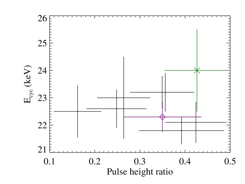
Figure 8.— Cyclotron line energy vs. ratio of secondary to primary pulse height. Each two-peaked pulse of the source is fitted with two Gaussians, modeling the primary and secondary pulses, and the pulse height ratio is the ratio of the heights of the fitted Gaussians. The average pulse height ratio is then computed for each time bin used in Section 4.2. The dip and flare are indicated as a purple diamond and a green star, respectively.

The CRSF width is also positively correlated with luminosity; this is in line with the observed correlation between CRSF energy and width seen in multiple sources and, indeed, across multiple sources (see, e.g., Coburn, 2001)). The correlation between $E_{\rm cyc}$ and $\sigma_{\rm cyc}$ is linear, with a slope of $0.9\pm 0.6$. The ratio of $\sigma_{\rm cyc}$ to $E_{\rm cyc}$ is, with the exception of the lowest-luminosity measurement from time bin 8, constant at $\sim 0.11$. The ratio of $E_{\rm cyc}$ to $\sigma_{\rm cyc}$ in a self-emitting atmosphere is given by Meszaros & Nagel (1985) as

$$\frac{\sigma_{\rm cyc}}{E_{\rm cyc}}\approx\left(8\ln 2\frac{kT_{\rm e}}{m_{\rm e}c^{2}}\right)^{\frac{1}{2}}|\cos\theta|$$ (19)

As $\theta$ is the angle between the magnetic field and the line of sight, $\cos\theta$ should not vary in phase-averaged spectra from a single observation. Thus, the interpretation is that a constant $E_{\rm cyc}/\sigma_{\rm cyc}$ ratio implies a relatively constant electron temperature of $\sim 1.3$ keV. The largest outlier is time bin 8, where the width of the CRSF drops to $\sim 1$ keV. The line is easily detected in this spectrum, appearing clearly in the residuals, but its shape is not fit well by the gauabs model. The cyclabs model, which uses a Lorentzian line profile, likewise does not fit the line well. This stems from the fact that there is no currently available physics-based model for the CRSF, and so the fitted width in these bins may not be physically meaningful. The CRSF depth is relatively stable throughout the observation, within errors, although the low width in time bin 8 results in only a lower bound for the optical depth.

The cyclotron line varies significantly with phase (Figure 6), and remains in-phase with the pulse profile in all continuum models. The behavior of the cyclotron line energy and width are comparable to the results of Clark et al. (1990) and Coburn (2001). The peak value of $E_{\mathrm{cyc}}$ is $\sim 24$ keV, similar to the peak cyclotron line energy seen in the time-resolved spectra. The CRSF width is also correlated with the pulse profile, although this is a more conditional statement than it was for the CRSF energy. The falling edge of the primary pulse is particularly problematic, as the CRSF width in that phase bin is exceptionally low, at $\sim 0.1-0.3$ keV. The depth in this bin is unbounded at the upper end due to the low width, and the line is overall much more poorly detected in comparison to the other phase bins, with its addition lowering the value of $\chi^{2}/{\rm dof}$ from $474.68/425$ to $445.04/423$ (compare to the peak of the main pulse, where the CRSF lowers $\chi^{2}/{\rm dof}$ from $689.74/435$ to $495.89/432$). However, beyond this one phase bin, the width shows a slight rise with phase, peaking with the primary pulse, and there is a hint of a correlation between the cyclotron line width and energy, similar to that seen in the phase-averaged spectra, but weaker. The depth follows the opposite pattern, with the highest-energy CRSF being one of the shallower features. The CRSF depth also displays the same asymmetry across the main pulse as seen in the other spectral parameters. Although Equation 19 predicts variation of $\sigma_{\rm cyc}/E_{\rm cyc}$ with luminosity within the pulse, no significant correlation can be found due to the large error bars.

6. Summary & Conclusions

We have carried out the first Suzaku observation of 4U 1538$-$522. Our comprehensive spectral analysis of the source examines the time-dependent and pulse-phase-dependent behavior of the source under a variety of spectral models. The dip-and-flare structure midway through the observation is associated with a significant increase in the line-of-sight absorption, with the timing and ionization characteristics of the absorption increase supporting the interpretation that the material that occulted the source was subsequently accreted onto one of the magnetic poles of the source, producing the observed flare. The intensity of the iron K$\alpha$ emission line at $6.4$ keV is found to correlate positively with luminosity in phase-averaged spectra, while the power-law index displays a negative correlation. A phase-resolved analysis additionally finds significant phase dependence in the spectral parameters, most notably finding a significant phase shift in the iron line intensity. The luminosity and phase dependence of the iron line, along with the lack of measurably high ionization, support the conclusion that the observed iron is, on average, approximately $0.7$ AU distant from the neutron star.

A positive correlation between the CRSF energy and luminosity is observed for the first time in this source. This correlation is moderately well explained by theoretical work by Becker et al. (2012), with the source accreting at sub-critical rates for most of the observation, increasing to above the critical luminosity during the flare. This is the first work that examines the behavior of the source at this high of a luminosity. Further work is necessary to properly compare this work to previous observations of the source, due primarily to differences in model choice and energy ranges used to calculate luminosity.

References

- Abbott (1982) Abbott, D. C. 1982, ApJ, 259, 282
- Becker & Wolff (2007) Becker, P. A., & Wolff, M. T. 2007, ApJ, 654, 435
- Becker et al. (2012) Becker, P. A., Klochkov, D., Schönherr, G., et al. 2012, A&A, 544, A123
- Becker et al. (1977) Becker, R. H., Swank, J. H., Boldt, E. A., et al. 1977, ApJ, 216, L11
- Boldt (1987) Boldt, E. 1987, Phys. Rep., 146, 215
- Clark (2000) Clark, G. W. 2000, ApJ, 542, L131
- Clark et al. (1994) Clark, G. W., Woo, J. W., & Nagase, F. 1994, ApJ, 422, 336
- Clark et al. (1990) Clark, G. W., Woo, J. W., Nagase, F., Makishima, K., & Sakao, T. 1990, ApJ, 353, 274
- Coburn (2001) Coburn, W. 2001, Phd, University of California, San Diego
- Crampton et al. (1978) Crampton, D., Hutchings, J. B., & Cowley, A. P. 1978, ApJ, 225, L63
- Davison et al. (1977) Davison, P. J. N., Watson, M. G., & Pye, J. P. 1977, MNRAS, 181, 73P
- Ferrigno et al. (2011) Ferrigno, C., Falanga, M., Bozzo, E., et al. 2011, A&A, 532, A76
- Finger et al. (2009) Finger, M. H., Beklen, E., Narayana Bhat, P., et al. 2009, arXiv:0912.3847
- Fürst et al. (2014) Fürst, F., Pottschmidt, K., Wilms, J., et al. 2014, ApJ, 780, 133
- Giacconi et al. (1974) Giacconi, R., Murray, S., Gursky, H., et al. 1974, ApJS, 27, 37
- Hemphill et al. (2013) Hemphill, P. B., Rothschild, R. E., Caballero, I., et al. 2013, ApJ, 777, 61
- Ilovaisky et al. (1979) Ilovaisky, S. A., Chevalier, C., & Motch, C. 1979, A&A, 71, L17
- Koyama et al. (2007) Koyama, K., Tsunemi, H., Dotani, T., et al. 2007, PASJ, 59, 23
- Larsson (1996) Larsson, S. 1996, A&AS, 117, 197
- Leahy et al. (1983) Leahy, D. A., Darbro, W., Elsner, R. F., et al. 1983, ApJ, 266, 160
- Makishima et al. (1987) Makishima, K., Koyama, K., Hayakawa, S., & Nagase, F. 1987, ApJ, 314, 619
- Makishima et al. (1999) Makishima, K., Mihara, T., Nagase, F., & Tanaka, Y. 1999, ApJ, 525, 978
- Manousakis et al. (2014) Manousakis, A., Walter, R., & Blondin, J. 2014, in European Physical Journal Web of Conferences, Vol. 64, European Physical Journal Web of Conferences, 2006
- Martínez-Núñez et al. (2014) Martínez-Núñez, S., Torrejón, J. M., Kühnel, M., et al. 2014, A&A, 563, A70
- Meszaros & Nagel (1985) Meszaros, P., & Nagel, W. 1985, ApJ, 299, 138
- Mihara (1995) Mihara, T. 1995, PhD thesis, Dept. of Physics, Univ. of Tokyo
- Mihara et al. (1998) Mihara, T., Makishima, K., & Nagase, F. 1998, Advances in Space Research, 22, 987
- Mukherjee et al. (2006) Mukherjee, U., Raichur, H., Paul, B., Naik, S., & Bhatt, N. 2006, Journal of Astrophysics and Astronomy, 27, 411
- Müller et al. (2013) Müller, S., Ferrigno, C., Kühnel, M., et al. 2013, A&A, 551, A6
- Nishimura (2014) Nishimura, O. 2014, ApJ, 781, 30
- Nowak et al. (2011) Nowak, M. A., Hanke, M., Trowbridge, S. N., et al. 2011, ApJ, 728, 13
- Palmeri et al. (2005) Palmeri, P., Kallman, T. R., Mendoza, C., Bautista, M. A., & Krolik, J. H. 2005, in American Institute of Physics Conference Series, Vol. 774, X-ray Diagnostics of Astrophysical Plasmas: Theory, Experiment, and Observation, ed. R. Smith, 75–82
- Poutanen et al. (2013) Poutanen, J., Mushtukov, A. A., Suleimanov, V. F., et al. 2013, ApJ, 777, 115
- Rawls et al. (2011) Rawls, M. L., Orosz, J. A., McClintock, J. E., et al. 2011, ApJ, 730, 25
- Reynolds et al. (1992) Reynolds, A. P., Bell, S. A., & Hilditch, R. W. 1992, MNRAS, 256, 631
- Robba et al. (2001) Robba, N. R., Burderi, L., Di Salvo, T., Iaria, R., & Cusumano, G. 2001, ApJ, 562, 950
- Rodes-Roca et al. (2010) Rodes-Roca, J. J., Page, K. L., Torrejón, J. M., Osborne, J. P., & Bernabéu, G. 2010, A&A, 526, A64
- Rodes-Roca et al. (2009) Rodes-Roca, J. J., Torrejón, J. M., Kreykenbohm, I., et al. 2009, A&A, 508, 395
- Rubin et al. (1997) Rubin, B. C., Finger, M. H., Scott, D. M., & Wilson, R. B. 1997, ApJ, 488, 413
- Schmidt et al. (2003) Schmidt, G. D., Harris, H. C., Liebert, J., et al. 2003, ApJ, 595, 1101
- Takahashi et al. (2007) Takahashi, T., Abe, K., Endo, M., et al. 2007, PASJ, 59, 35
- Tanaka (1986) Tanaka, Y. 1986, in Lecture Notes in Physics, Berlin Springer Verlag, Vol. 255, IAU Colloq. 89: Radiation Hydrodynamics in Stars and Compact Objects, ed. D. Mihalas & K.-H. A. Winkler, 198
- Tsujimoto et al. (2010) Tsujimoto, M., et al. 2010, Suzaku Memo 2010-03: Anomaly of XIS0 in June 2009, Tech. rep., JAXA
- Verner et al. (1996) Verner, D. A., Ferland, G. J., Korista, K. T., & Yakovlev, D. G. 1996, ApJ, 465, 487
- White et al. (1983) White, N. E., Swank, J. H., & Holt, S. S. 1983, ApJ, 270, 711
- Wilms et al. (2000) Wilms, J., Allen, A., & McCray, R. 2000, ApJ, 542, 914
- Wilms et al. (2010) Wilms, J., Lee, J. C., Nowak, M. A., et al. 2010, in Bulletin of the American Astronomical Society, Vol. 42, AAS/High Energy Astrophysics Division #11, 674