High order operator splitting methods based on an integral deferred correction framework
Andrew J. Christlieb 111Department of Mathematics and Department of Electrical and Computer Engineering, Michigan State University, East Lansing, MI 48824, USA. E-mail: christli@msu.edu Yuan Liu222Department of Mathematics, Michigan State University, East Lansing, MI 48824, USA. E-mail: yliu7@math.msu.edu Zhengfu Xu333Department of Mathematical Science, Michigan Technological University, Houghton, MI 49931, USA. E-mail: zhengfux@mtu.edu.
Abstract
Integral deferred correction (IDC) methods have been shown to be an efficient way to achieve arbitrary high order accuracy and possess good stability properties. In this paper, we construct high order operator splitting schemes using the IDC procedure to solve initial value problems (IVPs). We present analysis to show that the IDC methods can correct for both the splitting and numerical errors, lifting the order of accuracy by with each correction, where is the order of accuracy of the method used to solve the correction equation. We further apply this framework to solve partial differential equations (PDEs). Numerical examples in two dimensions of linear and nonlinear initial-boundary value problems are presented to demonstrate the performance of the proposed IDC approach.
Key Words: Integral deferred correction, initial-boundary value problem, high-order accuracy, operator splitting.
1 Introduction
In this paper we present high order operator splitting methods based on the integral deferred correction (IDC) mechanism. The methods are designed to leverage recent progress on parallel time stepping and offer a great deal of flexibility for computing the ordinary differential equations (ODEs). We focus on extending IDC theory to the case of splitting schemes on the IVP
| (1.1) |
and discuss the application in parabolic PDEs. Here, and .
In the case that (1.1) arises from a method of lines discretization of time dependent PDEs which describe multi-physics problems, we encounter high dimensional computation. For these problems, the splitting methods can be applied to decouple the problems into simpler sub-problems. Therefore, the main advantage of operator splitting methods are problem simplification, dimension reduction, and lower computational cost. Two broad categories can classify many splitting methods: differential operator splitting [1, 25, 32, 33] and algebraic splitting with the prominent example of the alternating direction implicit(ADI) method, which was first introduced in [9, 7, 30] for solving two dimensional heat equations. The main barrier in designing high order numerical methods based on the idea of splitting is the operator splitting error. To obtain high order accuracy via low order splitting method generally adds complexity to designing a scheme and stability analysis [14, 27, 18, 27, 26, 34, 12]. A recent work in [3] utilizes the spectral deferred correction (SDC) procedure to the advection-diffusion-reaction system in one dimension in order to enhance the overall order of accuracy. However, their work does not contain a proof that the corrections raise the order of the method.
In [10], a SDC method is first proposed as a new variation on the classical deferred correction methods [2]. The key idea is to recast the error equation such that the residual appears in the error equation in integral form instead of differential form, which greatly stabilizes the method. It is proposed as a framework to generate arbitrarily high order methods. This family of methods use Gaussian quadrature nodes in the correction to the defect or error, hence the method can achieve a maximal order of on grid points with corrections. This main feature of the SDC method made it popular and extensive investigation can be found in [10, 28, 21, 23, 22, 15, 16, 24]. Following this line of approach, the IDC methods are introduced in [6, 5, 4]. High order explicit and implicit Runge-Kutta (RK) integrators in both the prediction and correction steps (IDC-RK) are developed by utilizing uniform quadrature nodes for computing the residual. In [6, 5], it is established that using explicit RK methods of order in the correction step results in higher degrees of accuracy with each successive correction step, but only if uniform nodes are used instead of the Gaussian quadrature nodes of SDC. It is shown in [5] that the new methods produced by the IDC procedure are yet again RK methods. It is also demonstrated that, for the same order, IDC-RK methods possess better stability properties than the equivalent SDC methods. Furthermore, for explicit methods, each correction of IDC or SDC increases the region of absolute stability. Similar results are generalized to arbitrary order implicit and additive RK methods in [4]. Generally, for implicit methods based on IDC and SDC, the stability region becomes smaller when more correction steps are employed. It is believed that this is due to the numerical approximation of the residual integral. The primary purpose of this work is to apply the IDC methods to the low order operator splitting methods in order to obtain higher order accuracy.
The paper is organized as follows. In Section 2, we briefly review several classical operator splitting methods and show how these methods can be cast as additive RK (ARK) methods. In Section 3 we formulate the IDC methodology for application to operator splitting schemes. In Section 4, we prove that IDC methods can correct for both the splitting and numerical errors of ODEs, giving higher degrees of accuracy with each correction, where is the order of the method used in the correction steps. In section 5, as an interesting example, we will show how to use integral deferred correction for operator splitting (IDC-OS) schemes as a temporal discretization when solving PDEs. In Section 6 we carry out numerical simulations based on IDC methods for both linear and non-linear parabolic equations, and demonstrate that the new framework can achieve high order accuracy in time. In Section 7 we conclude the paper and discuss future work. We note that both the parallel time stepping version of IDC and the work presented in this paper are likely to benefit from the work in [20], and will be the subject of further investigation.
2 Operator splitting schemes for ODEs
In this section, we review several splitting methods which will serve as the base solver in the IDC framework. For differential operator splitting, such as Lie-Trotter splitting and Strang splitting, which happens at continuous level, we will apply appropriate numerical methods to the sub-problems and refer the whole approach as the discrete form of differential splitting. For both the differential splitting and algebraic splitting, we will show that each of the numerical schemes can be written as an ARK method. This insight is the first step required to apply the IDC methodology [4] to operator splitting schemes, which is the primary purpose of the present work.
2.1 Review of ARK methods
For IVP (1.1), when different -stage RK integrators are applied to each operator , the entire numerical method is called an ARK method. If we define the numerical solution after time steps as , which is an approximation to the exact solution , then one step of a -stage ARK method is given by
| (2.1) | |||||
| with | (2.2) |
and . An ARK method is succinctly identified by its Butcher tableau, as is demonstrated in Table 2.1.
In the following sections, we will explicitly write out the Butcher tableau for each operator splitting scheme and conclude that each of the operator splitting schemes considered in this work is indeed a form of ARK method.
2.2 Lie-Trotter splitting
We describe Lie-Trotter splitting for (1.1) in the case of in the right hand side functions. We consider a single interval . With first order Lie-Trotter splitting, (1.1) can be solved by two sub-problems:
| (2.3) |
The solution calculated from the first equation is used as the initial value of the second equation. Note that this splitting occurs on the continuous level. In order to define a discrete solver for (1.1), we need to choose a numerical scheme for solving each sub-problem. For example, if we use the backward Euler scheme to solve both equations, we obtain a scheme of the form
| (2.4) |
where denotes the numerical approximation for at time level . However, this approach only produces a first order approximation.
In order to make use of IDC methodology [4] to lift the order of accuracy of (2.4), we write a Butcher tableau for (2.4) in Table 2.2. Comparing the Butcher tableau for the Lie-Trotter splitting with the general form of the Butcher tableau of an ARK method, we can view the discrete form of Lie-Trotter splitting (2.4) as a 2-stage ARK method. This can be extended to the case of operators, where the resulting Butcher tableau would be a -stage ARK method.
| 0 | 0 | 0 | 0 | 0 | 0 | 0 |
|---|---|---|---|---|---|---|
| 1 | 0 | 1 | 0 | 0 | 0 | 0 |
| 1 | 0 | 1 | 0 | 0 | 0 | 1 |
| 0 | 1 | 0 | 0 | 0 | 1 |
2.3 Strang splitting
In this section, we consider the second order Strang splitting for the case of three operators to demonstrate how to construct Butcher tableaus for general differential operator splitting schemes. The case of operators can arise when splitting a stiff ODE into three sub-problems while maintaining second order accuracy in time.
We also focus on a single time step, . Second order Strang splitting for (1.1) reads as
| (2.5) |
Note that this splitting occurs on the continuous level, i.e. the temporal derivative for each sub-problem in (2.5) has yet to be discretized. If we discretize equations (2.5) with trapezoidal rule, we obtain an update of the form,
| (2.6) |
where . In Table 2.3, we write this scheme in the Butcher tableau. Comparing this with the Butcher tableau of the ARK methods, again we see that we can view the Strang splitting as a 5-stage ARK scheme.
| 0 | 0 | 0 | 0 | 0 | 0 | 0 | 0 | 0 | 0 | 0 | 0 | 0 | 0 | 0 | 0 | 0 | 0 | 0 | 0 | 0 |
|---|---|---|---|---|---|---|---|---|---|---|---|---|---|---|---|---|---|---|---|---|
| 0 | 0 | 0 | 0 | 0 | 0 | 0 | 0 | 0 | 0 | 0 | 0 | 0 | 0 | 0 | 0 | 0 | ||||
| 0 | 1 | 0 | 0 | 0 | 0 | 0 | 0 | 0 | 0 | 0 | 0 | 0 | 0 | 0 | 0 | 0 | ||||
| 0 | 0 | 1 | 0 | 0 | 0 | 0 | 0 | 0 | 0 | 0 | 0 | 0 | 0 | 0 | ||||||
| 0 | 0 | 0 | 0 | 0 | 0 | 0 | 0 | 0 | 0 | 0 | ||||||||||
| 1 | 0 | 0 | 0 | 0 | 0 | 0 | 0 | 0 | 0 | 0 | ||||||||||
| 0 | 0 | 0 | 0 | 0 | 0 | 0 | 0 | |||||||||||||
| 0 | 0 | 0 | 0 | 0 | 0 | 0 | 0 | 0 | 0 | 0 | 0 | 0 | 0 |
|---|---|---|---|---|---|---|---|---|---|---|---|---|---|
| 0 | 0 | 0 | 0 | 0 | 0 | 0 | 0 | 0 | 0 | ||||
| 0 | 1 | 0 | 0 | 0 | 0 | 0 | 0 | 0 | 0 | ||||
| 0 | 0 | 0 | 0 | 0 | 0 | ||||||||
| 1 | 0 | 0 | 0 | 0 | 0 | ||||||||
| 0 | 0 | 0 | 0 | ||||||||||
2.4 ADI splitting
The ADI method is a predictor-corrector scheme as a typical example of algebraic splitting, which happens after the discretization of equations. Here we are considering the discretized ODE version of the Peaceman-Rachford scheme [30] for (1.1). When , the ADI scheme takes the form
| (2.7) |
The Butcher tableau for the scheme (2.7) is shown in Table 2.5, and clearly, we see that we can view the ADI splitting scheme as a 2-stage ARK method.
| 0 | 0 | 0 | 0 | 0 | 0 | 0 |
|---|---|---|---|---|---|---|
| 0 | 0 | 0 | 0 | |||
| 1 | 0 | 1 | 0 | 0 | ||
| 0 | 1 | 0 | 0 |
3 Formulation of IDC-OS schemes
In this section, we review the formulation of IDC-OS presented in [4]. The authors [4] considered IDC methods for implicit-explicit (IMEX) schemes, where the non stiff part of the problem was treated explicitly, and the stiff part of the problem was treated implicitly. At present, our focus is on entirely implicit schemes.
We begin with some preliminary definitions. The starting point is to partition the time interval into intervals , , that satisfy
| (3.1) |
“macro”-time steps are defined by , and we permit them to vary with . Next, each interval is further partitioned into M sub-intervals , ,
| (3.2) |
with time step size . If Gaussian quadrature nodes are selected, as was originally done with the SDC method [10], varies with . Here, we only consider the case of uniform quadrature nodes, i.e. with for . Thus, without any ambiguity, we will drop the subscript on . Note that in what follows we will use superscript to denote the correction at a discrete set of time points and superscript to denote the continuous approximation given by passing a order polynomial through the discrete approximation. For simplicity, we drop the subscript for the description of the IDC procedure on “macro”-time interval . The whole iterative prediction-correction procedure is completed before moving on to the next time interval . The numerical solution at serves as the initial condition for the following interval .
-
1.
Prediction step : Use an -th order numerical method to obtain a preliminary solution to IVP (1.1)
(3.3) which is an -th order approximation to the exact solution
(3.4) where is the exact solution at for .
-
2.
Correction step : Use the error function to improve the accuracy of the scheme at each iteration. For to , ( is the number of correction steps):
-
(1) Denote the error function from the previous step as
(3.5) where is the exact solution and is an -th degree polynomial interpolating . Note that the error function, is not a polynomial in general.
-
(2) Denote the residual function as
(3.6) and compute the integral of the residual. For example,
(3.7) where are the coefficients that result from approximation of the integral by quadrature formulas and .
-
(3) Use an -th order numerical method to obtain an approximation to error vector
(3.8) where is the value of the exact error function (3.5) at time and we denote it as
(3.9) To compute by an operator splitting method consistent with the base method, we first express the error equation in a form consistent with original problem we are solving. We start by differentiating the error (3.5), together with (1.1)
Bring the residual to the left hand side, we have
(3.11) We now make the following change of variable,
(3.12) With this change of variable, we see that the error equation can be expressed as an IVP of the form,
(3.13) This is now in the form of (1.1) and we can apply the same operator splitting scheme to (3.13) that we applied to (1.1) and obtain the numerical approximation to . Recovering given is a simple procedure.
-
(4) Update the numerical solution as .
Remark 1 (The prediction step): For example, if we apply the discrete form of first order Lie-Trotter splitting (2.4) to (1.1) with , we have for ,
(3.14) Remark 2 (The correction step): As an example, if we use ADI splitting in the correction step, we will solve (3.13) with , we have for ,
(3.15) where
(3.16) for . Moreover, we note that we split the residual term equally for each operator in implementation.
-
4 Analysis of IDC-OS methods
In this section, we will discuss the error estimate for IDC-OS methods. Our analysis is similar to previous work of IDC-RK and IDC-ARK [6, 5, 4].
In section 4.1, we will establish that the IDC procedure can successfully reduce the splitting error for differential operator splitting methods where each sub-problem is solved exactly. In section 4.2, we continue by leveraging the ideas from the work in [4], and prove that the overall accuracy for the fully discrete methods is increased, as expected, with each successive correction. The second set of arguments apply to the discrete form of the differential operator splitting methods as well as the algebraic operator splitting methods. We present results for the stability regions of IDC-OS schemes in section 4.3. We remark that throughout this section, superscripts with a curly bracket denote the analytical functions related to solutions through differential splitting methods.
4.1 Splitting error: exact solutions to sub-problems
Differential operator splitting introduces a splitting error. If each sub-problem is solved exactly, the overall method only contains splitting error. Our starting point is to prove that IDC framework can reduce this splitting error. The primary result from this subsection is given by the following theorem.
Theorem 4.1.
Assume is the exact solution to IVP (1.1). Consider one time interval of an IDC method with . Suppose Lie-Trotter splitting (2.3) is used in the prediction step and the successive correction steps, and the sub-problems in each step are solved exactly. If and are at least differentiable, then the splitting error is of order after correction steps.
The proof of Theorem 4.1 follows by induction from the following two lemmas: Lemma 4.2 for the prediction step and Lemma 4.3 for the correction steps respectively.
Lemma 4.2.
The conclusion of Lemma 4.2 is simply a restatement of what the local error of splitting methods measures. The splitting error is for first order Lie-Trotter splitting [26].
Lemma 4.3.
Proof: We show the proof with the simple case . We have the error equation (3.13) after prediction and correction steps. Use the Lie-Trotter splitting method (2.3) to solve (3.13), we have
| (4.1) |
and
| (4.2) |
with defined in (3.16). Hence is the approximation of solved by the Lie-Trotter splitting method. It’s easy to see that
| (4.3) |
for . To prove , we examine the scaled variant
| (4.4) |
With this new notation, IVP (3.13) can be equivalently written as
| (4.5) |
with
| (4.6) |
Using the Lie-Trotter splitting method to solve IVP (4.5) will give us
| (4.7) |
and
| (4.8) |
with
| (4.9) |
is the approximation to through Lie-Trotter splitting. If , it is easy to verify that and . Similar as the work of IDC-RK in [6], one can further check that and . Therefore,
| (4.10) |
Notice that IVP (4.1) and (4.7) are both first order ODEs, and . Since is the solution to (4.7), is a solution to (4.1). Through the uniqueness of the solution for IVP, one can conclude that
| (4.11) |
Similarly, from IVP (4.2) and (4.8), one can further conclude
| (4.12) |
Thus (4.10) is equivalent to
| (4.13) |
i.e.
| (4.14) |
We now complete the proof of Lemma 4.3 for the case of Lie-Trotter splitting.
The conclusion in Theorem 4.1 also holds for Strang splitting method (2.5) and the proof is essentially the same as Lie-Trotter splitting. We have now demonstrated that IDC can lift the order of accuracy when each sub-problem is solved exactly, however, in practice, we usually do not have access to analytical solutions for these sub-problems. We will consider the fully discrete scheme in the next section.
4.2 Local truncation error: discrete solutions to sub-problems
A fully discrete solution introduces additional error beyond the splitting error. In this section, we turn to analyzing fully discrete IDC-OS schemes and begin with some preliminary definitions [6].
Definition 4.4.
(Discrete differentiation) Consider the discrete data set, , with defined as uniform quadrature nodes in (3.2). We denote as the -th degree Lagrangian interpolant of :
| (4.15) |
An -th degree discrete differentiation is a linear mapping that maps to , where
| (4.16) |
This linear mapping can be represented by a matrix multiplication , where and ,
Definition 4.5.
The Sobolev norm of the discrete data set is defined as
| (4.17) |
where is the identity matrix operating on .
Definition 4.6.
(smoothness of a discrete data set) A discrete data set possesses degrees of smoothness if is bounded as , with defined as the step size in the sub-interval where .
As discussed in section 2, all the listed operator splitting schemes are a form of ARK methods. Therefore, we can use the framework of the IDC-ARK schemes in [4] to enhance the order of the discretized scheme. Hence, we shall describe only what is needed for clarity when extending the results of the work in [4] to the fully implicit case under consideration here. For further details, we refer the reader to [5, 4]. The theorems below apply to lifting the order of algebraic splitting as well as the discrete form of differential splitting. The splitting error discussed in Theorem 4.1 is directly related to the local truncation error. We note that the results in the following theorem can be generalized to all IDC-OS schemes which can be written as a form of ARK method and the proof is quite similar.
Theorem 4.7.
Let be the solution to IVP (1.1). Assume , and are at least differentiable with respect to each argument, where . Consider one time interval of an IDC method with and uniformly distributed quadrature points. Suppose an -th order ARK method (2.1) is used in the prediction step and -th order ARK methods are used in the successive correction steps. Let . If , then the local truncation error is of order after correction steps.
The proof of Theorem 4.7 follows by induction from the following lemmas for the prediction and correction steps. For clarity, similar as [4], we will sketch a proof for Lie-Trotter splitting.
Lemma 4.8.
(prediction step) Consider an -th order ARK method for (1.1) on , with (M+1) uniformly distributed quadrature points. and satisfy the smoothness requirement in Theorem 4.7 and let be the numerical solution. Then,
-
(1) The error vector satisfies .
-
(2) The rescaled error vector has degrees of smoothness in the discrete sense.
Proof: (1) is obvious. We will prove (2) next. We drop the superscript as there is no ambiguity. Applying the discrete form of the Lie-Trotter splitting (2.4) to IVP (1.1) with , we have
| (4.18) |
i.e.
| (4.19) |
Performing Taylor expansion of at , we get
| (4.20) |
on the other hand, the exact solution satisfies
Subtracting (4.20) from (4.2) gives
where is the error at . Denote
| (4.22) |
and
| (4.23) |
We will use an inductive approach with respect to the degree of the smoothness to investigate the smoothness of the rescaled error vector , and
| (4.24) |
First of all, has at least zero degrees of smoothness in the discrete sense since . Assume has degrees of smoothness, we will show has degrees of smoothness, from which we can conclude has degrees of smoothness.
By assuming that and have at least degrees of smoothness, we can conclude and have at least degrees of smoothness, which implies and have at least degrees of smoothness. Therefore will have degrees of smoothness. Also, will have at least degrees of smoothness. Therefore, has degrees of smoothness. Therefore, has degrees of smoothness. Notice that , we complete the inductive approach and conclude has degrees of smoothness.
Before investigating the correction step for IDC-OS schemes, we describe some details for the error equations first. Notice that the error equation after (k-1) correction steps has the form of (3.11), with the notation , we actually implement the problem (3.13) on time interval via discrete Lie-Trotter splitting as follows
| (4.26) |
through which is updated. Furthermore, we can update by (3.12) and (3.7). Similarly, if we apply Lie-Trotter splitting to the scaled error equation (4.5) over the time interval , we have
| (4.27) |
from which we obtain and further .
Lemma 4.9.
(correction step) Let and satisfy the smoothness requirements in Theorem 4.7. Suppose and has degrees of smoothness in the discrete sense after the -th correction step. Then, after the -th correction step using an -th order ARK method and ,
-
(1) .
-
(2) The rescaled error vector has degrees of smoothness in the discrete sense.
Proof: The proof of Lemma 4.9 is similar as Lemma 4.8, but more tedious. Similar as in [4], we outline the proof here and present the difference between the proof of IDC-OS and IDC-RK, IDC-ARK in Proposition 4.10, we refer the reader to [5] for details.
-
1.
Substract the numerical error vector from the integrated error equation
(4.28) and make necessary substitution and expansion via the rescaled equations.
-
2.
Bound the error by an inductive approach.
The following proposition is about the equivalence of the rescaled error vector and unscaled error vectors for Lie-Trotter splitting. We remark that the proof of this proposition shows the difference of the proof between IDC-OS and IDC-RK in [5], IDC-ARK in [4].
Proposition 4.10.
Consider a single step of an IDC scheme constructed with the Lie-Trotter splitting scheme for the error equation, assume the exact solution , and satisfies the smoothness requirement in Theorem 4.7, then for a sufficiently smooth error function , the difference between the Taylor series for the exact error and the numerical error is after correction steps.
Proof: Notice that the left and right hand side terms of the rescaled error equation (4.5) is , applying the discrete form of Lie-Trotter splitting scheme (2.4) to (4.5) will result in
| (4.29) |
Since
| (4.30) |
The proof is complete if the following argument holds.
| (4.31) |
which is also equivalent to
| (4.32) |
We will prove (4.32) by induction. (4.32) holds for since the initial condition for the error equation is set as . Assume (4.31) holds for , then
On the other hand, Taylor expanding at will give us
Compare (4.2) and (4.2), we can conclude
| (4.35) |
Similar approach to the second equation in (4.26) and (4.27) will result in
| (4.36) |
which completes the inductive proof for (4.32).
4.3 Stability
In this subsection, we study the linear stability of the proposed IDC-OS numerical schemes. As is common practice [13], we consider the test problem
| (4.37) |
and observe how the numerical scheme behaves for different complex values of . Without loss of generality, we will assume that , and we’ll consider a single time step of length . The stability region of a numerical method is then defined as
| (4.38) |
An additional complication comes from the fact that an operator splitting scheme requires a splitting of the right hand side of (4.37) into parts. For simplicity, we’ll consider the special case of with , and we further assume that for simplicity.
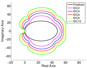
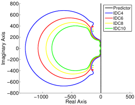
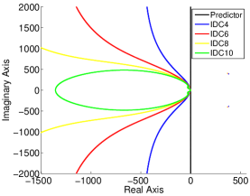
In Figure 4.1 we present stability regions for IDC-OS methods based on three separate base solvers: Lie-Trotter splitting, Strang splitting and ADI splitting. The stability region of Lie-Trotter splitting with IDC procedure is everywhere outside the curves, and the stability regions for Strang splitting and ADI is the finite region inside the curves. The number in the legend denotes the order of the method. For example, “IDC4” represents fourth order methods achieved by the IDC-OS schemes; for Lie-Trotter splitting, we require three correctors to attain fourth-order accuracy, whereas Strang and ADI splitting only require a single correction. Our first observation is that of the three base solvers, Lie-Trotter splitting is the only solver that retains an infinite region of absolute stability, whereas Strang splitting and ADI reduce to finite regions of absolute stability.
Consistent with other implicit IDC methods, the stability regions for our implicit IDC-OS methods decreases as the number of correction steps increases. We have observed that larger stability regions can be found if we include more quadrature nodes for evaluating the integral of the residual.444For all simulations used in this work, we use 13 uniformly distributed interior nodes for evaluating the residual integral in the error equation. This leads us to conjecture that a more accurate numerical approximation of the residual integral is important in finding larger stability regions.
(a)
(b)
(c)
5 Application of IDC-OS schemes to parabolic PDEs
In this section, we will discuss how to apply the IDC-OS framework to the parabolic problem of the form
| (5.1) |
The methods can be generalized to a high dimensional setting, but in this work we restrict our attention to two dimensions. For differential splitting methods, it is quite straightforward to apply IDC-OS schemes if we solve (5.1) via method of lines. One can obtain semi-discrete ODE systems which have the same form as (1.1) after spatial discretization. It is natural to assume one operator, say is related to the terms in direction, while is related to the terms in direction. As for algebraic splitting, one major difficulty for applying the IDC-OS framework to PDEs is how to handle the boundary and initial conditions for the error equation. In the following context, we will introduce one ADI formulation which can effectively deal with those issues. For simplicity, we only discuss the case when there is no nonlinear source in (5.1), i.e. .
Classical ADI starts by applying second-order Crank-Nicholson time discretization to the continuous PDE (5.1), this process produces a semi-discrete scheme
| (5.2) |
where is the time step, , and . On a two dimensional structured mesh, we choose to use the central difference approximation (of orders or ) for approximating the spatial operators , , and , and we denote them by , respectively. If the spatial discretization is performed on an grid, there are equations in the form of (5.2). We denote as the unknowns in vector form, then we can write these equations into matrix multiplication where boundary conditions are also incorporated,
where , , , and are the boundary terms. Notice that, different from [8], we enforce the boundary conditions strictly in the scheme. It is easy to verify that the method given in (5) is second order accurate in time. Specifically, if we use six order central difference for spatial derivatives such as in the numerical simulations, the local truncation error of (5) is . Denoting
| (5.4) | |||
(5) is equivalent to
| (5.5) |
To set up an ADI scheme, we follow [8] by adding one term to both sides of (5.5), which results in
| (5.6) |
Then it is straightforward to factor (5.6) as
| (5.7) |
Let us consider the second term on the right hand side of (5.7). Observe that
| (5.8) |
and that and both carry a in them, we see that the term . Hence, the second term on the right hand side of (5.7) is the same order as the truncation error, thus can be dropped. Therefore, the scheme reduces to
| (5.9) |
To solve (5.9), a two-step method was proposed in [9, 30],
| (5.10) |
However, to be symbolically consistent, symmetric and suited for IDC method, we choose to split the boundary values in the following way,
| (5.11) |
with boundary terms defined as
| (5.12) |
It should also be pointed out that the boundary values are associated with boundary functions at time and , instead of , therefore there is no error introduced from intermediate values on the boundary. This is important for setting the boundary conditions when solving the error equation of IDC when we combine the ADI scheme with the IDC methodology. Because the Dirichlet boundary conditions of (5.1) are exact and accounted for in the formulation of the prediction, therefore, the boundary terms will not show up in the correction steps.
6 Numerical examples
In this section, we present numerical results for the proposed implicit IDC-OS schemes on a variety of examples of the parabolic initial-boundary value problem (5.1), where our aim is to demonstrate the efficiency of the proposed time-stepping methods. We begin with two linear examples of (5.1), and then present an example of the heat equation with a nonlinear forcing term. Our final two examples come from mathematical biology: the Fitzhugh-Nagumo reaction-diffusion model and the Schnakenberg model.
Our present work is in two-dimensions, and every result is performed on a square domain with a cartesian grid. We solve (5.1) using -th order central difference for the spatial discretization in order that the temporal error is dominant in the measured numerical error.
Example 1. Linear example: Dirichlet boundary conditions. We solve initial boundary value problem (5.1) with constant coefficient in the domain . Initial condition is taken as and time dependent boundary conditions are . Therefore, (5.1) has the exact solution . represents the number of spatial grids in - and -direction. is the time steps used in the time interval where is end time. is the number of correction steps. is the exact solution and as the numerical solution. We solve Example 1 by first order Lie-Trotter splitting (2.4), second order Strang splitting (2.6) and ADI splitting (5.11) and all the splitting performed via dimensional fashion, the numerical error are shown in Table 6.6, Table 6.7 and Table 6.8 respectively. We can clearly conclude that the schemes achieve the designed order with IDC methodology, i.e. with one more correction step, the order of the scheme increases by 1 for Lie-Trotter splitting, while the order of the scheme increases by 2 for Strang splitting and ADI splitting.
| Number of time steps | ||||||||
|---|---|---|---|---|---|---|---|---|
| Correction | order | order | order | order | ||||
| = 0 | 1.53e-5 | – | 1.15e-5 | 0.99 | 9.24e-6 | 0.98 | 7.70e-6 | 1.00 |
| = 1 | 1.90e-7 | – | 1.09e-7 | 1.93 | 7.08e-8 | 1.93 | 4.94e-8 | 1.97 |
| = 2 | 3.10e-9 | – | 1.47e-9 | 2.59 | 8.06e-10 | 2.69 | 4.87e-10 | 2.76 |
| Number of time steps | ||||||||
|---|---|---|---|---|---|---|---|---|
| Correction | order | order | order | order | ||||
| = 0 | 3.02e-5 | – | 1.69e-5 | 2.02 | 1.08e-5 | 2.01 | 7.55e-6 | 1.96 |
| = 1 | 7.15e-7 | – | 2.45e-7 | 3.72 | 1.04e-7 | 3.84 | 5.20e-8 | 3.80 |
| = 2 | 3.64e-10 | – | 8.06e-11 | 5.24 | 2.28e-11 | 5.66 | 7.16e-12 | 6.35 |
| Number of time steps | ||||||||
| Correction | order | order | order | order | ||||
| = 0 | 3.68e-5 | – | 2.07e-5 | 2.00 | 1.32e-5 | 2.00 | 9.20e-6 | 2.00 |
| = 1 | 4.49e-7 | – | 2.08e-7 | 2.67 | 1.03e-7 | 3.13 | 5.07e-8 | 3.91 |
| = 2 | 1.18e-7 | – | 1.69e-8 | 6.74 | 4.74e-9 | 5.71 | 1.59e-9 | 5.98 |
Example 2. Linear example: periodic boundary conditions. In this example, we will solve (5.1) when , and the initial condition . We compute errors using the difference between two successive refinements:
| (6.1) |
where describes the number of time steps.
Again, we present results using three splitting options: Lie-Trotter, Strang and ADI splitting. Convergence studies are presented in Tables 6.9, 6.10 and 6.11, and we can also observe that the schemes achieve the designed order. Note that the numerical error for the two correctors when is not reliable in the cases of Strang and ADI splitting because of precision limitation.
| Number of time steps | ||||||||
| Correction | order | order | order | order | ||||
| = 0 | 4.65e-3 | – | 2.35e-3 | 0.98 | 1.18e-3 | 0.99 | 5.94e-4 | 0.99 |
| = 1 | 1.85e-4 | – | 5.68e-5 | 1.70 | 1.63e-5 | 1.80 | 4.44e-6 | 1.88 |
| = 2 | 3.47e-6 | – | 6.55e-7 | 2.41 | 1.19e-7 | 2.46 | 1.88e-8 | 2.66 |
| Number of time steps | ||||||||
|---|---|---|---|---|---|---|---|---|
| Correction | order | order | order | order | ||||
| = 0 | 5.24e-5 | – | 1.31e-5 | 2.00 | 3.29e-6 | 1.99 | 8.22e-7 | 2.00 |
| = 1 | 3.30e-9 | – | 2.06e-10 | 4.00 | 1.29e-11 | 4.00 | 8.04e-13 | 4.00 |
| = 2 | 5.80e-12 | – | 4.90e-14 | 6.89 | 7.77e-16 | 5.98 | 1.11e-16 | 2.81 |
| Number of time steps | ||||||||
|---|---|---|---|---|---|---|---|---|
| Correction | order | order | order | order | ||||
| = 0 | 7.77e-5 | – | 1.94e-5 | 2.00 | 4.85e-6 | 2.00 | 1.21e-6 | 2.00 |
| = 1 | 1.93e-8 | – | 1.20e-9 | 4.00 | 7.52e-11 | 4.00 | 4.70e-12 | 4.00 |
| = 2 | 1.43e-11 | – | 2.23e-13 | 6.01 | 3.56e-15 | 5.96 | 1.04e-16 | 5.10 |
Example 3. Nonlinear equation with Dirichlet boundary conditions. We now test the proposed IDC-OS methods on a nonlinear example of (5.1) with a known exact solution.
| (6.2) |
on the domain . The exact solution to this problem is . Given that we have an exact solution, all our numerical tests use exact boundary conditions from this solution.
An IDC-OS solver for (6.2) requires a definition for how the splitting will be performed. Here, we choose to split the problem into three pieces: and are the same as linear case, while contains the remaining non-linear terms,
| (6.3) |
We use Newton-iteration to solve the discretized version of .
In Tables 6.12 and 6.13 we present results from applying the IDC-OS method with Lie-Trotter and Strang splitting as the base solvers. In each case, we can see the successful increase of order after each correction: one in the case of Lie-Trotter splitting, and two in the case of Strang splitting.
In this work, we do not present results for IDC-OS methods based on ADI splitting for non-linear problems due to their computational complexity. The high-order differential operator splitting methods discussed here are much simpler than what would arise from using even low-order ADI splitting.
| Number of time steps | ||||||||
| Correction | order | order | order | order | ||||
| = 0 | 6.88e-3 | – | 5.16e-3 | 1.00 | 4.13e-3 | 1.00 | 3.44e-3 | 1.00 |
| = 1 | 7.31e-4 | – | 4.33e-4 | 1.82 | 2.87e-4 | 1.84 | 2.03e-4 | 1.90 |
| = 2 | 1.60e-5 | – | 6.95e-6 | 2.90 | 3.59e-6 | 2.96 | 2.06e-6 | 3.05 |
| Number of time steps | ||||||||
|---|---|---|---|---|---|---|---|---|
| Correction | order | order | order | order | ||||
| = 0 | 9.21e-5 | – | 5.20e-5 | 1.99 | 3.34e-5 | 1.98 | 2.33e-5 | 1.99 |
| = 1 | 3.04e-6 | – | 8.96e-7 | 4.25 | 3.38e-7 | 4.37 | 1.56e-7 | 4.24 |
| = 2 | 1.87e-8 | – | 3.22e-9 | 6.11 | 8.33e-10 | 6.06 | 2.84e-10 | 5.90 |
Example 4. Fitzhugh-Nagumo reaction-diffusion model. A simple mathematical model of an excitable medium is Fitzhugh-Nagumo (FHN) equations [11]. FHN equations with diffusion can be written as
| (6.4) |
where , are the diffusion coefficients for activator and inhibitor respectively, and is a real parameter. We consider the classical cubic FHN local dynamics [19, 29]
| (6.5) |
where , and are dimensionless parameters. We perform the numerical experiment for (6.4) and (6.5) on the domain with periodic boundary conditions. The parameters are chosen as following, , , , , , and . The initial condition is
| (6.6) |
| (6.7) |
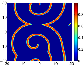
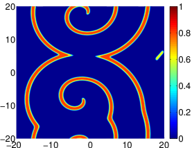
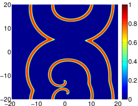
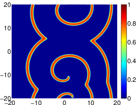
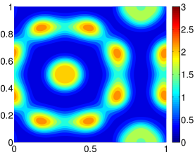
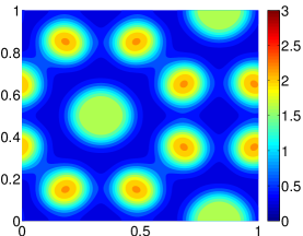
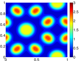
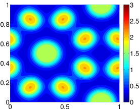
The domain is partitioned with a grid. Figure 6.2 shows the numerical solution to the concentration of the activator solving by Lie-Trotter splitting scheme, with three operators similar as Example 3. We observe the spiral waves at , which show a good agreement with the reference solutions. The computational step size is in all cases. We remark that, because the lower order schemes suffer more from the numerical error of diffusion than higher order ones, the pattern for look more consistent if we take a smaller computational time step size or a more refined mesh. Similar patterns can also be obtained by IDC-OS scheme based on Strang splitting.

(a1)
(a2)

(a3)
(b1)
(b2)

(b3)
(c1)

(c2)
(c3)
Remark. Figure 6.3 shows the order of accuracy for Fitzhugh-Nagumo reaction-diffusion model (6.4) at , in which we clearly observe the order increase of IDC-OS scheme with successive correction steps. However, for a more stiff parameter such as , order reduction phenomena is observed in the convergence study. Similar observation is made in the Example 5 on Schnakenberg model. How to approximate the residual integral and design a robust solver for stiff ODEs is an open question. Recently work in [20], the authors proposed a highly accurate solver based on an approximation of the integral of the residual as a linear combination of exponentials on uniform quadrature nodes. Their method is shown to do a good job of attaining high order of accuracy with correction steps and preserving the stability region of the original implicit time integrator which is used as the base scheme.

Example 5. Schnakenberg model. The Schnakenberg system [31] has been used to model the spatial distribution of a morphogen. It has the following form
| (6.8) |
where and represents the concentration of activator and inhibitor, with and as the diffusion coefficients respectively. , and are rate constants of biochemical reactions. Following the setup in [17], we take the initial conditions as
| (6.9) | ||||
| (6.10) |
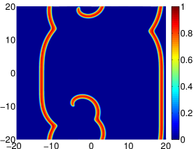
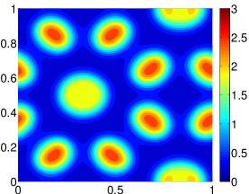
and the boundary conditions are periodic. The parameters are , , , and . The computational domain is . The numerical simulations with Lie-Trotter splitting is performed on a spatial grid and the numerical dynamical process of the concentration of the activator at different times are shown in Figure 6.4, we can observe that the initial data are amplified and spreads, leading to thew formation of spot pattern. The computational time step size is chosen as . We also note that similar patterns can be obtained by IDC-OS scheme based on Strang splitting.

(a1)
(a2)

(a3)
(b1)
(b2)

(b3)
(c1)

(c2)
(c3)
7 Conclusion
In this paper, we have provided a general temporal framework for the construction of high order operator splitting methods based on the integral deferred correction procedure. The method can achieve arbitrary high order via solving correction equation whereas reduce the computational cost by taking the advantage of operator splitting. Error analysis and numerical examples for IDC-OS methods are performed to show that the proposed IDC framework successfully enhances the order of accuracy in time. A study on order reduction for very stiff problems will be part of our future work.
Acknowledgments
AJC supported in part by AFOSR grants FA9550-11-1-0281, FA9550-12-1-0343 and FA9550-12-1-0455, NSF grant DMS-1115709, and MSU Foundation grant SPG-RG100059. ZX is supported by NSF grant DMS-1316662. Additionally, the authors would like to thank Prof. William Hitchon and Dr. David Seal for helpful comments on this work.
References
- [1] K. Bagrinovskii and S. Godunov. Difference schemes for multidimensional problems (in russian). Doklady Akademii Nauk, 115:431–433, 1957.
- [2] K. Bohmer and H. Stetter. Defect correction methods. Theory and Applications Springer-Verlag, Wien, 1984.
- [3] A. Bourlioux, A. Layton, and M. Minion. High-order multi-implicit spectral deferred correction methods for problems of reactive flow. Journal of Computational Physics, 189(2):651–675, 2003.
- [4] A. Christlieb, M. Morton, B. Ong, and J.-M. Qiu. Semi-implicit integral deferred correction constructed with additive runge–kutta methods. Communications in Mathematical Sciences, 9:879–902, 2011.
- [5] A. Christlieb, B. Ong, and J.-M. Qiu. Comments on high order integrators embedded within integral deferred correction methods. Communications in Applied Mathematics and Computational Science, 4(1):27–56, 2009.
- [6] A. Christlieb, B. Ong, and J.-M. Qiu. Integral deferred correction methods constructed with high order runge-kutta integrators. Mathematics of Computation, 79(270):761–783, 2010.
- [7] J. Douglas. On the numerical integration of by implicit methods. Journal of the Society for Industrial and Applied Mathematics, 3(1):42–65, 1955.
- [8] J. Douglas and S. Kim. On accuracy of alternating direction implicit methods for parabolic equations. Preprint, 1999.
- [9] J. Douglas and D. Peaceman. Numerical solution of two-dimensional heat-flow problems. AIChE Journal, 1(4):505–512, 1955.
- [10] A. Dutt, L. Greengard, and V. Rokhlin. Spectral deferred correction methods for ordinary differential equations. BIT Numerical Mathematics, 40(2):241–266, 2000.
- [11] P. C. Fife et al. Mathematical aspects of reacting and diffusing systems. Springer Verlag., 1979.
- [12] J. Geiser. Higher-order difference and higher-order splitting methods for 2d parabolic problems with mixed derivatives. 2(67):3339–3350, 2007.
- [13] E. Hairer, S. Nørsett, and G. Wanner. Solving ordinary differential equations, volume 2. Springer, 1991.
- [14] E. Hansen and A. Ostermann. High order splitting methods for analytic semigroups exist. BIT Numerical Mathematics, 49(3):527–542, 2009.
- [15] J. Huang, J. Jia, and M. Minion. Accelerating the convergence of spectral deferred correction methods. Journal of Computational Physics, 214(2):633–656, 2006.
- [16] J. Huang, J. Jia, and M. Minion. Arbitrary order krylov deferred correction methods for differential algebraic equations. Journal of Computational Physics, 221(2):739–760, 2007.
- [17] W. Hundsdorfer and J. Verwer. Numerical solution of time-dependent advection-diffusion-reaction equations, volume 33. Springer, 2003.
- [18] H. Jia and K. Li. A third accurate operator splitting method. Mathematical and Computer Modelling, 53(1):387–396, 2011.
- [19] J. Keener and J. Sneyd. Mathematical Physiology: I: Cellular Physiology, volume 1. Springer, 2010.
- [20] D. Kushnir and V. Rokhlin. A highly accurate solver for stiff ordinary differential equations. SIAM Journal on Scientific Computing, 34(3):A1296–A1315, 2012.
- [21] A. Layton. On the choice of correctors for semi-implicit picard deferred correction methods. Applied Numerical Mathematics, 58(6):845–858, 2008.
- [22] A. Layton and M. Minion. Implications of the choice of quadrature nodes for picard integral deferred corrections methods for ordinary differential equations. BIT Numerical Mathematics, 45(2):341–373, 2005.
- [23] A. Layton and M. Minion. Implications of the choice of predictors for semi-implicit picard integral deferred correction methods. Communications in Applied Mathematics and Computational Science, 2(1):1–34, 2007.
- [24] Y. Liu, C.-W. Shu, and M. Zhang. Strong stability preserving property of the deferred correction time discretization. Journal of Computational Mathematics, 26(5):633–656, 2008.
- [25] G. Marchuk. Some application of splitting-up methods to the solution of mathematical physics problems. Aplikace Matematiky, 13(2):103–132, 1968.
- [26] R. McLachlan and G. R. Quispel. Splitting methods. Acta Numerica, 11:341–434, 2002.
- [27] R. McLachlan and G. R. Quispel. Geometric integrators for odes. Journal of Physics A: Mathematical and General, 39(19):5251, 2006.
- [28] M. Minion. Semi-implicit spectral deferred correction methods for ordinary differential equations. Communications in Mathematical Sciences, 1(3):471–500, 2003.
- [29] D. Olmos and B. Shizgal. Pseudospectral method of solution of the fitzhugh–nagumo equation. Mathematics and Computers in Simulation, 79(7):2258–2278, 2009.
- [30] D. W. Peaceman and H. H. Rachford, Jr. The numerical solution of parabolic and elliptic differential equations. Journal of the Society for Industrial and Applied Mathematics, 3(1):28–41, 1955.
- [31] J. Schnakenberg. Simple chemical reaction systems with limit cycle behaviour. Journal of theoretical biology, 81(3):389–400, 1979.
- [32] G. Strang. On the construction and comparison of difference schemes. SIAM Journal on Numerical Analysis, 5(3):506–517, 1968.
- [33] G. Strang. Approximating semigroups and the consistency of difference schemes. Proceedings of the American Mathematical Society, 20(1):1–7, 1969.
- [34] M. Thalhammer. High-order exponential operator splitting methods for time-dependent schrödinger equations. SIAM Journal on Numerical Analysis, 46(4):2022–2038, 2008.