The Core Collapse Supernova Rate from the SDSS-II Supernova Survey

Abstract

We use the Sloan Digital Sky Survey II Supernova Survey (SDSS-II SNS) data to measure the volumetric core collapse supernova (CCSN) rate in the redshift range $(0.03<z<0.09)$. Using a sample of 89 CCSN we find a volume-averaged rate of $1.06{\pm}0.19\times 10^{-4}\frac{(h/0.7)^{3}}{(\mathrm{yr}\mathrm{Mpc}^{3})}$ at a mean redshift of $0.072\pm 0.009$. We measure the CCSN luminosity function from the data and consider the implications on the star formation history.

1 Introduction

Supernovae of the observational Types Ib, Ic and all Type II are the result of core collapse events in massive stars. Because the interval from massive star formation to CCSN is brief on astronomical time scales, the CCSN distribution in space and time traces the formation of massive stars, a process that is not currently well understood. Study of the stellar population in galaxies shows an increasing rate of star formation with redshift up to $z\approx 0.5$ proportional to the phenomenological rate formula $(1+z)^{\beta}$ with $\beta$ having values in the range 2.5 to 3.9 (Hopkins, 2004; Schiminovich, 2005; Le Floc’h, 2005; Hopkins&Beacom, 2006; Rujopakarn, 2010; Cucciati, 2012) depending on the redshift and wavelength ranges considered. Comparisons between the star formation and CCSN rate densities show that the redshift dependence of the two agree well up to redshift of about 1.0 with higher values of $\beta$ as in Horiuchi (2011).

However, there is confusion on the absolute comparison between the two rates: when the overall star formation rate density and initial mass function are used to predict the rate at which massive stars form, it ought to match the rate at which CCSN occur, given our current understanding of stellar evolution. Horiuchi and collaborators in Horiuchi (2011) note an apparent discrepancy between the two absolute rates with the star formation implying a much higher CCSN rate than is observed. This disagreement could be caused by a very large misunderstanding of stellar evolution, a large change in the initial stellar mass function, or large population of dim or extincted CCSN that evade detection as a function of redshift that preserves the observed redshift dependence. Botticella and collaborators in Botticella (2012) conclude that the star formation rate derived from H$\alpha$ is too small by a factor of 2, which would exacerbate further the discrepancy reported in Horiuchi (2011). Recently Mathews and collaborators in Mathews (2014) have looked at this and conclude that there may no “supernova rate problem” at all.

The goal of this work is to measure the CCSN rate more accurately than was previously possible, taking advantage of the large spatial volume sampled by and the uniform observing conditions of the SDSS-II SNS described in Frieman (2008), to help resolve this confusion. More properly we will measure the CCSN rate density, but we often use the common short hand of “rate” for the rate density. The SDSS-II SNS was designed to detect type Ia supernovae (SNIa) in the so-called “redshift desert”, where previous supernova data were lacking. Likewise, the survey’s design allows our CCSN rate measurements to probe an intermediate redshift range where no prior CCSN rate has been published. Our CCSN data span the region $0.03<z<0.09$. Combined with other CCSN rate measurements, our measurement helps anchor the CCSN rate desnity versus redshift curve.

The CCSN rate density is also valuable input to supernova cosmology studies. Increasingly large samples of photometric supernova light curves are being gathered with only a small fraction of the objects having simultaneous spectral data for the identification of supernova types. Precise knowledge of the CCSN rate will be needed to understand and quantify the level of CCSN contamination in a sample of SNIa selected with only photometry.

The current generation of supernova surveys have greatly increased the accuracy and time resolution of supernova observations. The SDSS-II SNS is part of this cohort, along with the Supernova Legacy Survey (SNLS) and Southern intermediate redshift ESO Supernova Search (STRESS). SDSS-II SNS and SNLS were designed primarily to measure SNIa candidates for cosmology, but incidentally detected a large, well–characterized sample of CCSN. STRESS, on the other hand, was explicitly designed as a supernova rate survey for both SNIa and CCSN, though it did not quite have the same commitment of observational resources as SNLS and SDSS-II SNS. The SNLS analysis of Bazin (2009) and the STRESS analysis of Botticella (2008) are today’s state of the art CCSN rate density measurements. This work adds to the CCSN rate results for the current generation of surveys.

Surveys in search of SNIa provide an opportunity to measure the CCSN rate density, as the observation and image processing pipeline designed to discover SNIa will incidentally detect a nearly equal number of CCSN. We have employed this approach using data from the SDSS-II SNS, from which we extracted ${\sim}10000$ CCSN candidates, although we use only a fraction of this sample to measure the CCSN rate at redshift less than $0.1$.

In the next sections we describe the SDSS-II SNS and the important ancillary data we obtained from the SDSS-III BOSS project described in Eisenstein (2011); Dawson (2013), how we characterize candidates, our model for the efficiency of detecting CCSN, the selections that we make to count observed CCSN, corrections we apply to that count, sources of uncertainty, the rate calculation, discuss our result, and conclude.

2 The SDSS-II SNS and SDSS-III BOSS

We only briefly describe the SDSS-II SNS here. Full details are given in Frieman (2008); Fukugita (1996); Gunn (1998); York (2000); Gunn (2006). Sako (2014) makes the entire data sample publically available and gives more details about its composition. For the SDSS-II SNS, a 300 $\mathrm{deg}^{2}$ region of sky, designated the Equatorial stripe and also known as ‘Stripe 82’, was targeted for imaging once every two days; however, viewing conditions only allowed imaging of the entire stripe once every four days, on average. To detect supernovae within the search region, images from each night were compared to a previously observed SDSS template image of the same region of the sky to identify transient objects. To reduce the number of candidates to consider, a catalog of known quasars, variable stars and active galactic nuclei (AGNs) was used to exclude variable objects that are known not to be supernovae. We account later for these known variables by reducing our observing area. We hand scanned the images of the excluded AGNs, and observed no additional variable objects within them. Also, most objects within the solar system are rejected by software; their proper motion is so large that their position shifts significantly in the few minutes between $g-$, $r-$ and $i-$band exposures.

Initially the observed variable objects were forwarded to a team of human scanners within the collaboration. Images of each object were visually inspected by one or more scanners, who registered their judgment on whether the object might be a supernova. Many transient signals are obviously not supernovae, including fast moving objects, poor image subtractions, and telescope artifacts. Also, when a variable object was detected in more than one year of observation, it was excluded from the sample, as supernovae are extremely unlikely to be detected over such a long period of time. As the survey progressed, exclusion of these non-supernovae became increasingly automated, so that a greater fraction of objects forwarded to the scanners were subsequently identified as possible supernovae. A key change made after our first observing season is that software observed variable objects were only forwarded to human scanners after two observations, rather than one. This reduced the number of human scanned objects by nearly a factor of ten, but led to little change in the number of supernova candidates, and no change for variable objects with peak magnitude brighter than magnitude 21 in the $r-$band. The photometry for the supernova candidates is described in Holtzman (2008).

As the SDSS-II SNS was designed to detect and measure SNIa, it produced an excellent sample for measuring the rate density of SNIa. Analysis of the SDSS-II SNS data in Dilday (2008) and Dilday (2010) identified a rate sample of over 500 SNIa candidates, approximately half of which were spectroscopically confirmed. The remainder were typed by a template fitting algorithm, shown in Monte Carlo simulations to add only about 5% uncertainty to the rate measurement due to false positives.

For the CCSN rate measurement presented here, we make use of methods developed in Dilday (2008). In general, CCSN are much more diverse than SNIa, and therefore tools to identify CCSN candidates from photometry alone are not as well developed as for SNIa. However, we can make use of the current consensus view that SNIa and CCSN together comprise nearly the entire set of observed supernovae besides “peculiar” SNIa and CCSN with very unusual light curves, both of which are rare. Thus we are able to establish the CCSN rate by first counting generic supernova light curves, then subtracting the relatively easier to identify SNIa from the sample using Dilday’s methods. The possibility of exotic supernova types that are neither CCSN nor SNIa does exist, but their numbers as a fraction of all supernovae detected to date is unlikely to be an important consideration. Uncertainty in the CCSN rate due to exotic supernovae, using our best estimate at their presence in our sample, is negligible compared to other uncertainties.

The SDSS-III BOSS described in Eisenstein (2011); Dawson (2013) project provides important ancillary data for this result. While SNIa not observed spectroscopically can have an estimate of their redshift based on their peak brightness and colors, this is not possible for the much more diverse CCSN. Unknown redshifts for supernova candidates observed only photometrically would be a dominant uncertainty for the CCSN rate, while limiting CCSN candidates to those that were observed spectroscopically would limit the size of the sample leading to a large statistical uncertainty on the CCSN rate. The SDSS-III BOSS project provided a way out of this dilemma by spectroscopically measuring the redshift of almost all $r\lesssim 21$ galaxies that are hosts to SDSS-II SNS supernova candidates.

At the beginning of the SDSS-III BOSS project, we compiled a list of suggested targets. This was a complete list of galaxies, not observed spectroscopically in the SDSS-II SNS, that are nearest to a supernova candidate in angular distance and nearest in isophotal distance. Isophotal distance measures the candidate’s distance from the galaxy center, as a fraction of the galaxy’s isophotal size along the galaxy-candidate axis. When a galaxy is nearest to a candidate in both angular and isophotal distance at a redshift smaller than 0.1, confidence is high, better than 97%, that it is the galaxy in which the supernova candidate actually occurred. For more details on the selection of the galaxies targeted by SDSS-III BOSS see Olmstead (2013); Campbell (2013); Sako (2014).

A small fraction of the recommended targets could not be observed due to technical reasons, usually fiber collisions, and observational constraints, usually the requested target’s brightness was below the reliable measurement threshold. SDSS-III BOSS discovered that some, less than 5%, of the targets were variable stars or quasars, which unsurprisingly means that some of the variable light sources observed by our survey were not a supernova at all. For the remainder, which appear to be typical galaxies, the BOSS team measured redshifts. The data were taken with the BOSS spectrograph described in Smee (2013) and processed by the BOSS pipeline described in Bolton (2012).

Our sample has a heterogeneous sample of spectra taken by many different instruments of varied natures. We make use of these spectra to identify the supernova type and measure the redshift. In the redshift range of interest, less than 0.1, the supernova identification for SNIa is very secure and the uncertainty on the redshift is negligible.

3 Supernova Detection Efficiency Model

Our rate measurement begins with the complete set of $9933$ SDSS-II SNS candidate light curves with associated redshifts smaller than 0.3 or no good measure of their redshifts, as produced by the analysis pipeline outlined in the preceding section. The SDSS-II SNS used relatively loose criteria for identifying a supernova candidate. Therefore, the candidate set from which we begin includes a large number of variable objects that are not supernovae, such as variable stars, quasars and other active galaxies, or perhaps even novae within the Milky Way.

To separate supernovae from other variable object types, we employed the phenomenological light curve fitting method used by the SNLS in Bazin (2009). They model observed supernova brightness in each pass band as a function of time using the formula:

$$f(t)=A\frac{e^{-(\frac{t-t_{0}}{\tau_{F}})}}{(1+e^{-(\frac{t-t_{0}}{\tau_{R}})})}$$ (1)

We fit for the four parameters $A$, the overall amplitude of the light curve, $t_{0}$, roughly the time of peak luminosity, $\tau_{R}$, the rate of flux increase long before the peak, and $\tau_{F}$, the rate of flux decrease long after the peak. We fit in the $r-$band and the maximum of the function defines the peak brightness which we will use to model our detection efficiently. Details of the fitting procedure are given in Taylor (2011).

Of 9933 light curves processed, the fit failed to converge on 62 candidates. Of those, 60 candidates recorded null or negative flux in the $r-$band for all epochs; those 60 are discarded. These were identified by human scanners in the first season based on an initial, later improved, photometric image subtraction. Visual inspection confirms that the remaining two display oscillatory features not characteristic of supernovae, as shown in Figure 1. The uncertainty due to excluding non-converging fits is negligible compared to other sources of uncertainty.

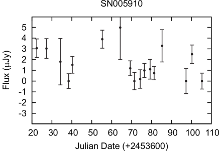
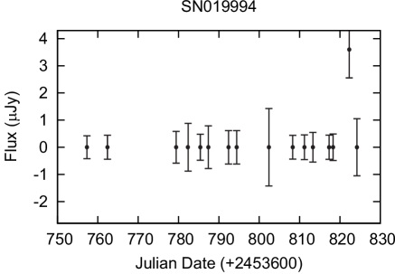
Figure 1: SDSS-II SNS candidate $r-$band light curves are shown for two objects which the light curve model did not converge to a best fit.

The supernova model adapted from Bazin (2009) can be fit to virtually any light curve; however, the fit will be poor for light curves without a clear, dominant peak. To measure the quality of the fit, we again follow the method of Bazin by fitting a second model to each light curve, which is just the best-fit constant flux.

When the constant flux fit has a chi-squared comparable to the chi-squared for the model fit, the object either is not a supernova, or the data are too noisy to identify it as a supernova. In either case, we remove such objects from the rate sample. The model and constant flux chi-squared are directly compared, even though the model has three more degrees of freedom, as both functions are fit to the same number of data points, which in almost all cases is large compared to the number of fit parameters. To quantify this comparison, we assign each light curve a flatness score, $\Lambda$, defined by:

$$\Lambda\equiv\frac{\chi^{2}_{model}}{\chi^{2}_{model}+\chi^{2}_{const}}$$ (2)

The value of $\Lambda$ ranges from zero for the best measured, obvious supernovae, to one for light curves that show no supernova features. Figure 2 shows the distribution of $\Lambda$ for all SDSS-II SNS candidates with redshift less than 0.09. It is bimodal, with a large peak near $\Lambda=0.5$, and a smaller peak near $\Lambda=0$.

To test the correlation between flatness score and object type, we examine the $\Lambda$ distribution for two candidate sub-samples: core collapse supernovae and active galaxies, both of which have been confirmed through spectroscopic analysis, as described in Sako (2008, 2011). We find that spectroscopically confirmed CCSN, the middle plot in Figure 2, are concentrated near $\Lambda=0$, as expected, while the bottom plot shows that confirmed AGN are concentrated near $\Lambda=0.5$.

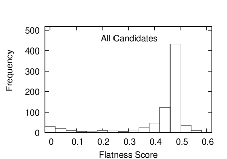
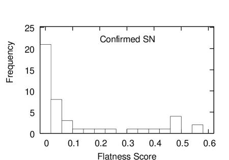
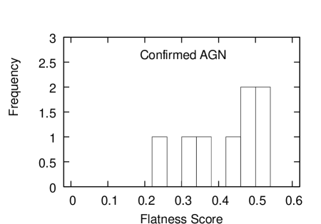
Figure 2: Flatness score, as defined in the text, distribution is shown for all candidates (top), for spectroscopically confirmed supernovae (middle), and for confirmed AGN (bottom). All data have $z<0.09$.

Based on these distributions we define supernova candidates to have $\Lambda_{c}<0.354$. The systematic uncertainty of this choice is discussed below. A representative selection of light curves, confirmed AGN at various redshifts, excluded by the flatness score requirement are shown in Figure 3, and

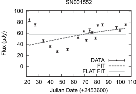
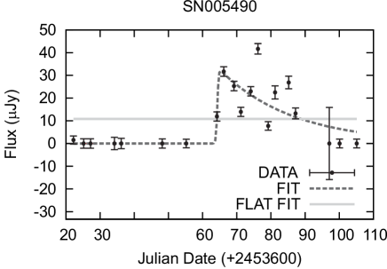
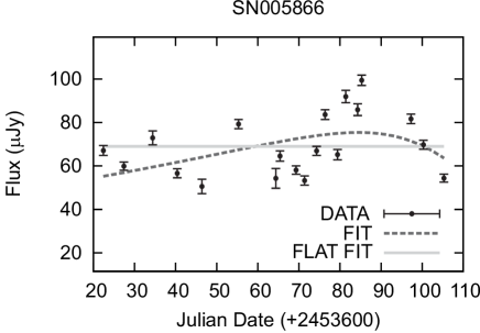
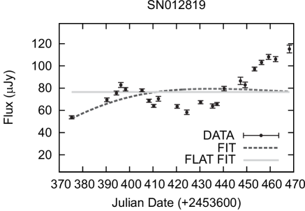
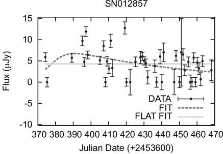
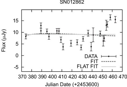
Figure 3: Above are examples of confirmed AGN light curves at various redshifts, with the the constant flux fit with a full line and the supernova model described in the text with a dashed line. All these candidates were excluded by the flatness requirement. Only the r-band is shown for clarity.

Figure 4 shows examples of accepted light curves.

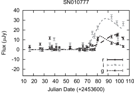
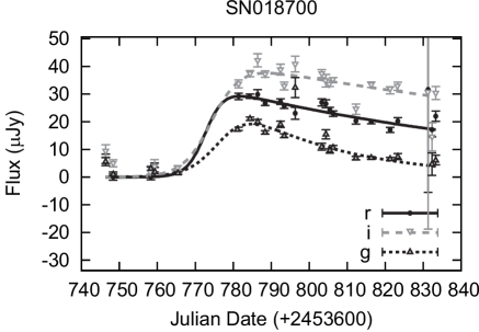
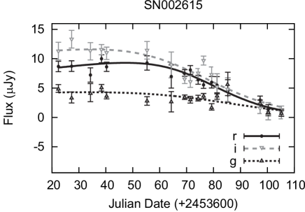
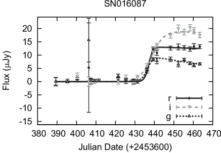
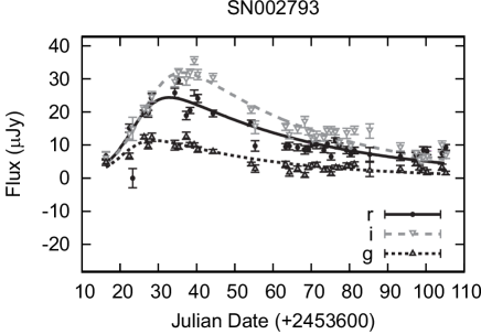
Figure 4: Above are examples light curves accepted into the core collapse supernova rate sample. The lines show the SN model fit described in the text.

The magnitude limit, beyond which a supernova is too dim for the survey to detect, is not a sharp boundary. There is a range of magnitudes, due to light curve shape, observing conditions, and survey cadence, over which supernovae have a finite probability of detection. We refer to this function as our survey’s detection efficiency. We model the detection efficiency as a function of the supernova’s peak apparent magnitude as seen in the SDSS $r-$band. The form of the model efficiency function, $\epsilon(m)$ is:

$$\epsilon(m)=\frac{1}{2}\left[1-\mathrm{erf}(\frac{m-m_{E}}{\sigma_{E}})\right]$$ (3)

This form is simply the convolution of a normal distribution of width $\sigma_{E}$ with a step function whose transition occurs at $m_{E}$.

To measure $m_{E}$ and $\sigma_{E}$ we start with the sample of SN candidates that have peak magnitudes bright enough that our detection efficiency is nearly one. We take this magnitude to be 21; see below for further discussion. The cumulative number of candidates with peak magnitude $m$ smaller than $m_{E}$, $N_{p}(m)$, should have the form:

$$N_{p}(m)=p_{0}+p_{1}10^{0.6m}+p_{2}10^{0.8m}+p_{3}10^{1.0m}+p_{4}10^{1.2m}$$ (4)

where the coefficients $p_{i}$ are determined by fitting the observed distribution shown in Figure 5.

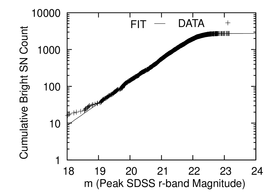
Figure 5: The cumulative bright supernova candidate count, $N_{p}(m)$, versus the peak $r-$band magnitude ($m$). The fit shown with a line and discussed in the text determines the efficiency model.

Equation 4 is derived by first expressing the SN rate, $\rho_{SN}$, as a function of luminosity distance, $D$, and expanding $\rho_{SN}(D)$ with a Taylor series in $D$. The luminosity distance is then in turn expressed in terms of the distance modulus, $\mu$, according to:

$$D=(10\mathrm{pc})\mbox{ }10^{0.2\mu}$$ (5)

Integrating over the sample volume and simplifying then yields Equation 4, approximated to fourth order in $(10\ \mathrm{pc})/D$.

Once the best fit $N_{p}(m)$ is obtained for the bright portion of the rate sample, it is compared to the actual number of candidates at all magnitudes, $N_{a}(m)$. The form of $N_{p}(m)$ should be nearly the same at dimmer magnitudes as at bright magnitudes, since each cohort in apparent magnitude includes objects at a wide range of distances.

Next we fit the actual number of candidates, $N_{a}(m)$, to

$$N_{a}(m)=\int_{-\infty}^{m}\!\epsilon(a)N_{p}(a)\,\mathrm{d}a$$ (6)

which includes the effect of the efficiency. The parameters of $N_{p}(m)$, the model population function, are held fixed at the values fitted to the bright sub-sample, while the parameters of $\epsilon(m)$, the efficiency function, are allowed to float. The resulting, best fit efficiency model is displayed in Figure 6.

Figure 6: The model supernova detection efficiency as a function of the peak brightness for all SN candidates. The model fit shown with a line is used to correct the observed count of CCSN.

Details for the efficiency model can be found in Taylor (2011).

With the detection efficiency model in hand, we weight each supernova candidate according to the inverse of the efficiency based on its peak apparent magnitude. The corrected supernova count is then the sum of these weights, for all accepted candidates. In addition, we find the uncertainty in each candidates’ weight by taking the standard deviation of 1000 random trials. For each trial the candidate’s peak magnitude is drawn from a Gaussian distribution of width given by the uncertainty in the candidate’s peak magnitude weighted by the detection efficiency.

The resulting, corrected redshift distribution is shown in Figure 7. Also displayed in the figure is the uncorrected, raw distribution. The actual supernova count is expected to

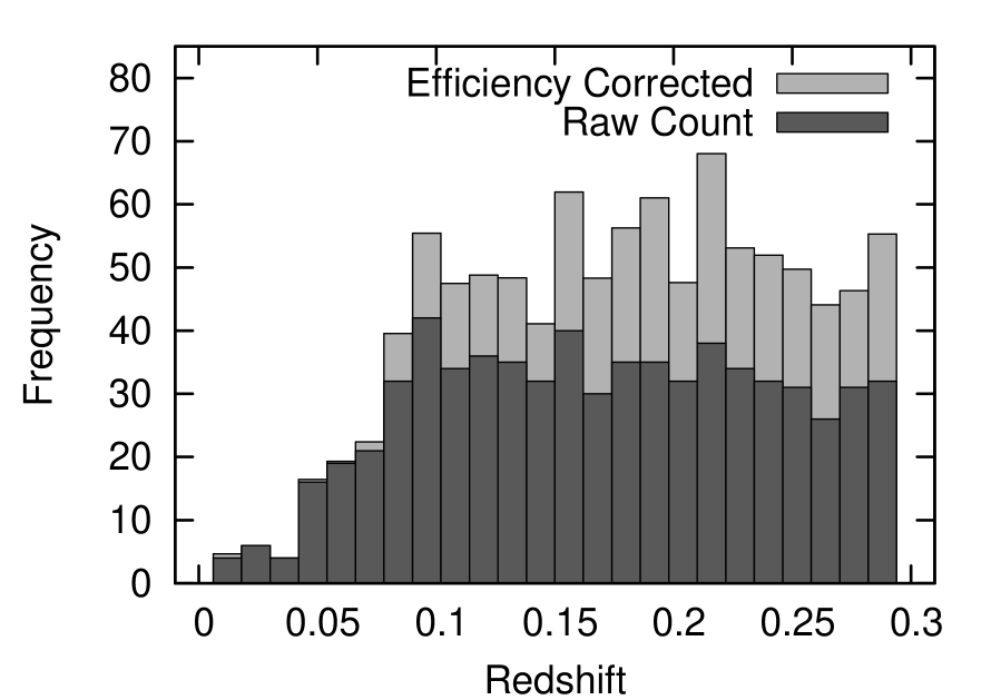
Figure 7: The redshift distribution of the CCSN rate sample is shown, sub-luminous sample excluded, before and after the efficiency correction.

increase as approximately the third power of redshift, because of the increasing volume sampled. However, beyond $z\approx 0.1$, an increasingly large fraction of the CCSN population is at magnitudes where the survey has very low or zero detection efficiency.

We need a redshift as a distance measure. Spectroscopic redshift of the supernova itself is preferred, but when that is not available we instead use the spectroscopic redshift of the host galaxy, or a photometric redshift estimate of the host galaxy as a last resort. However, in a few cases no spectra were taken of the supernova, the host galaxy is too faint to detect, or for technical reasons the redshift of the host galaxy is not measured, thus we have no guidance at all for the candidate’s distance. We remove candidates from the sample due to lack of redshift information, treating all of them as non-detections. Figure 8

Figure 8: The peak apparent magnitude distribution, in SDSS $r-$band, is shown for SN candidates excluded from the rate sample for lack of redshift information on top, and below for the SN cadidates in the rate sample with redshift information.

shows the peak magnitude distribution of such candidates, showing that the majority of these are at the edge of our detection limit. Also the figure shows the peak magnitude distribution of all the candidates that pass all the other slections, but have a redshift determination. By treating candidates with no redshift as non-detections, we are implicitly assuming that they are beyond our upper redshift cut of 0.09, and we attempt to justify this assumption below.

4 CCSN Rate Selections

We select only candidates which fall in the Right Ascension (RA) and Declination (DEC) for which the SDSS-II SNS had full coverage during its three seasons. The RA had a ragged edge night-to-night due to time and weather limitations and we simply chose the range that was covered on 100% of the observing nights.

The candidate light curve has to be successfully fit by our light curve model as described above. Candidates have to pass the flatness score test described above. We truncate the rate sample at $z=0.09$ to limit the effect of low detection efficiency discussed above. Galaxies with $z<0.03$ are not homogeneously distributed, leading to a distortion in the apparent spatial distribution of supernovae. To avoid this effect, which violates assumptions of our efficiency model, we exclude any supernova candidate with redshift less than 0.03 from the rate sample.

We need to remove SNIa for our CCSN rate measure. Fortunately, the SDSS-II SNS has sophisticated methods for identification of SNIa, as they are the primary targets of interest for the survey’s cosmology mission. Objects which display properties most similar to SNIa, and which are suitable for spectroscopic observation, were submitted to the SDSS-II SNS partner observatories. The spectra obtained are subjected to a cross-correlation analysis, comparing them with template spectra for SNIa, CCSN and other object types. The spectroscopic target selection process and spectrum analysis are described in Zheng (2008). Those which match the SNIa templates are marked as confirmed SNIa in the SDSS-II SNS database, and we remove all such candidates from our CCSN rate sample.

The SDSS-II SNS identified many more supernova candidates than available spectroscopic resources could observe, therefore methods were developed to identify SNIa using only the photometric data from SDSS-II SNS itself. Sako (2008, 2011) describes this process in detail; we only summarize here. Observed light curves are fit to a variety of supernova templates, selecting the supernova type which fits the data best. Those candidates identified as SNIa by this classification program are marked as photometric SNIa in the SDSS-II SNS database, and we remove all such candidates from our CCSN rate sample. Over 93% of the SNIa candidates removed from our sample are identified spetroscopically.

After fitting light curves to the Bazin (2009) model, we excluded all candidates where the model peak occurs in the first or last 10 days of a observing season, 2005, 2006, and 2007, or where there are no observations before or after the time of the fit peak. The Julian date ranges included are shown in Table 1, summing to a total survey time of 264 days, or 0.723 years.

Table 1: Survey Time Ranges Included in CCSN Rate Measurement

Observing Season	Julian Date Range	Days
2005	53622 - 53705	83
2006	53974 - 54068	94
2007	54346 - 54433	87
Total		264

As a supernova’s luminosity decreases, the effective volume of the survey also decreases. This means that the intrinsically dimmest supernovae are always under-represented in any large volume of space. We exclude from the rate sample any supernova with peak absolute magnitude of $-15.0$ or dimmer in the SDSS $r-$band assuming a flat spectral distribution. We call these the sub-luminous sample. As all other supernova rate measurements to date suffer the same limitation, either implicitly or via an explicit luminosity requirement such as ours, the results will still be comparable. The final measurement is therefore more properly the “bright core collapse rate density.” Note that here we are explicit as to what this means for this result, while this is usually implicit in all other supernova rate measurements. We discuss the implications of this requirement further in Section 8.

Table 2 summarizes the selections we have made on our initial large sample to arrive at the 89 candidates we use for the CCSN rate density measurement.

Table 2: The SDSS-II SNS CCSN Rate Sample.

Selection	Number
Candidate Within RA-DEC Range	9933
Fit Light Curve	9871
$0.03<z<0.09$	808
Flatness Score Test	205
Not Type Ia Supernova	157
Within Observing Season	100
Not Sub-Luminous	89
Accepted CCSN Candidates	89

5 Corrections

The SDSS-II SNS does not detect all supernovae that occur. Weather, lunar phase, proximity to other celestial objects, and many other factors can result in non-detection. To compensate for this effect, we constructed an efficiency model as described in Section 3. Each candidate in the rate sample is then weighted by the inverse of the survey detection efficiency, as a function of supernova peak apparent magnitude. The weighting scheme corrects the base sample count upward by 7.44 supernovae. The correction is relatively small as we have confined our sample to a redshift range in which we are highly efficient at detecting CCSN that are not sub-luminous.

The observed luminosity of a supernova may be less than its actual luminosity due to extinction. However, dust in each supernova’s host galaxy, or perhaps even in the local environment of the supernova itself, is more difficult to measure. This local extinction is represented by the parametrization of Cardelli (1989), which quantifies extinction with two parameters, $A_{V}$ and $R_{V}$.

We employ the model developed by Hatano (1998), who simulated an ensemble of host galaxies at random inclinations, and placed model supernovae within them approximating the spatial distribution of observed supernovae. Dust along the resulting line of sight determined the extinction of each model supernova. The resulting $A_{V}$ distribution is roughly exponential, ${P}(A_{V})\approx\frac{1}{\tau_{V}}e^{-\frac{A_{V}}{\tau_{V}}}$, with exponent $\tau_{V}=0.50\pm 0.03$, where we use a standard $R_{V}=3.1$. Details of how we correct the observed supernova count due to extinction can be found in Taylor (2011). The extinction correction is small, less than 3% of the measured rate, and because of poorly quantified uncertainties in the extinction model, we count 100% of this correction as a systematic uncertainty. There is evidence at higher redshifts that extinction for CCSN is much larger Melinder (2012), and this is another reason for our redshift selection maximum at 0.09.

The results of efficiency and extinction corrections are summarized in Table  3.

Table 3: Corrections to the CCSN Rate Sample Size.

Reason	Adjustment	Sample Size
Base Rate Sample		89.00
Efficiency Correction	7.44	96.44
Extinction Correction	2.11	98.55
Corrected Rate Sample		98.55

6 Sources of Uncertainty

Table  4 summarizes the sources of statistical and systematic errors. We discuss the systematic errors in more detail below.

To study systematic effects due to inherent assumptions in the efficiency model, we compared it to another efficiency model. This second model represented the detection efficiency as exactly 100% for bright objects, zero for dim objects, and follows a cosine function of the object peak magnitude in the transition region between. The efficiency correction of 6.13 produced by this alternative model is consistent with the correction from our base model, 7.44, and the difference is small compared to the statistical uncertainty on the base model which is calculated by summing the uncertainty on the weight assigned to each candidate, $\pm 7.43$. We conclude that the efficiency correction is not strongly dependent on the exact shape of the assumed detection efficiency function, and we assign the statistical error on the model we use, which is large compared to the differences among these, as the systematic uncertainty due to the efficiency correction.

We have cross checked this efficiency model with a SNANA, a public supernova analysis and simulation package described in Kessler (2009b), based simulation of CCSN in the SDSS-II SNS. It agrees that we are fully efficient for the bright CCSN, peak magnitude brighter than 21, and rolls off smoothly to being completely inefficient for dimmer CCSN, peak magnitude dimmer than 23. We can obtain arbitrary precision with this simulation, but do not have a clear way to assess its systematic uncertainty. The simulation is based on a finite set of CCSN templates which are unlikely to span the diversity of real CSSN. The uncertainty from the empirically–derived efficiency described above is a better estimate of our lack of understanding of our efficiency model than any procedure that we have thought of based on a likely incomplete simulation.

The identification of supernovae based on flatness score, $\Lambda$, also may introduce systematic uncertainty. The number of confirmed AGN in the target redshift region is small, and they may not be representative of all AGN. To estimate this uncertainty, we measure the rate at which confirmed supernovae are rejected by the flatness score requirement, and the rate at which confirmed AGN are accepted by the same requirement; 100% of both numbers is taken as systematic uncertainty. Adding these two sources in quadrature, we find systematic uncertainty of $\pm 6.22$ in the supernova count due to misidentification. This value is large compared to our best guess of exotic supernovae types that could be contaminating our sample. Li (2011) notes that in a volume–limited sample of supernovae lightcurves, 5% of the SNIa sample is the distinct “2002cx-like” objects, which we estimate as the number of truly exotic objects that would not fall clearly under our two categories of SNIa or CCSN. This result translates to $2.4$ objects which we add in quadrature to misidentification uncertainty to get $\pm 6.67$ as an uncertainty on the supernova count. We get a similar estimate, $\pm 3.5$ if rather we assume that truly exotic objects are Type Iax supernovae, of which 2002cx is thought to be a member, as suggested in Foley (2013). Type Iax are thought to be roughly 30% of the SNIa sample in a given volume, but their impact is reduced due to our brightness threshold which about half of the dimmer Type Iax would not pass. There is an even smaller change, $\pm 2$ if we vary the flatness cut from $0.3$ to $0.4$ from its nominal value of 0.354.

At low redshifts, $(z<0.1)$, where CCSN can be detected with high efficiency, the combined photometric and spectroscopic identification of SNIa is very accurate. Our simulation tests in the SNIa rate measurement found that less than 1% of SDSS-II SNS candidate SNIa are actually CCSN, as found in Dilday (2010). CCSN are more than three times as numerous as SNIa in a given volume of space, therefore excluding survey-identified SNIa from our sample should remove less than 0.3% of CCSN from the rate calculation; an insignificant effect compared to other sources of uncertainty.

Though the SDSS-III BOSS data greatly improved the accuracy of redshift estimates, there are still some supernovae in the sample with only photometric redshifts. To estimate the resulting uncertainty, we compared spectroscopic and photometric redshift measurements for those candidates where both were available. The resulting error is counted as the number of candidates that would be moved into or out of the redshift range of interest when replacing the photometric value with the spectroscopic value. This yields $\pm 10\%$ systematic uncertainty in the supernova count, due to incorrect redshift.

For the good light curves without any reasonable measure of their redshift we make an estimate of the number that could violate our assumption that they were beyond the redshift range of our rate sample. We modeled each individual redshift as a Gaussian with mean and width equal to the mean and width of the redshift distribution of the sample all 1074 light curves that pass all our other selection, have good redshifts, and peak magnitudes within one of the candidate without redshift. Many of these are SNIa at redshifts greater than 0.1. We then integrated the area of these 149 Guassians between 0.03 and 0.09 and find a sum of less than one. Our best guess is that a very small number of these, compared to the 10% count uncertainty due to incorrect redshifts, could possibly enter our sample and we assign no systematic uncertainty due to removing them. Our assertion that the almost all of the sample without good redshifts are beyond the redshift range of our rate sample.

The supernova rate density is measured by the supernova count divided by survey time and volume. The error on the time and volume is negligible compared to error in the supernova count. We use the co-moving volume that encloses the sample of supernovae. Uncertainty in cosmological parameters could make a small contribution to uncertainty in the co-moving volume, and hence uncertainty in the supernova rate density. To probe the effect of varying cosmological parameters on co-moving volume, we employed the iCosmos cosmological distance calculator, developed by Vardanyan (2011). The SDSS-II SNS cosmology study found a 5% uncertainty in $\Omega_{m}$ in Kessler (2009a), which translates to approximately 0.3% uncertainty in comoving volume at $z=0.09$. We ignore this. Kessler (2009a) also found approximately 10% uncertainty in $w$, the dark energy equation of state parameter, which translates to a 1.3% uncertainty in comoving volume at $z=0.09$. The effect of uncertainty in $w$ is small, but it is significant enough to account for in sources of uncertainty for the CCSN rate, and we have included it in the uncertainty tabulation.

Table  4 summarizes the sources of statistical and systematic uncertainty; they are added in quadrature for a total uncertainty estimate.

Table 4: Sources of Uncertainty in the CCSN Rate

Source of Uncertainty	Uncertainty in SN Count	% Uncertainty
Statistical Uncertainty	10.31	10.6%
Efficiency Correction	7.43	7.5%
Extinction Correction	2.11	2.1%
Identification by Flatness	6.67	6.8%
Redshift Uncertainty	10.00	10.2%
Volume due to Cosmology Parameters		1.3%
All Systematic Uncertainties		14.6%
Total Uncertainty		18.0%

7 CCSN Rate Calculation

The survey volume is calculated as the difference between two sections of a sphere, each subtended by the solid angle given by the chosen limits on right ascension and declination. Because the declination range lies within $1.25^{\circ}$ of the celestial equator, we can use the small angle approximation for $\Delta\theta$ given by:

$$V=\frac{1}{3}(\Delta\theta)(\Delta\phi)(D_{c2}^{3}-D_{c1}^{3})$$ (7)

where $D_{c1}$ and $D_{c2}$ are the co-moving distances at $z=0.03$ and $z=0.09$, respectively. The right ascension range, which gives $\Delta\phi$, of the survey is $-50^{\circ}$ to $50^{\circ}$. Note that we further correct by a factor of $1/(1+z)$ in the survey volume integration to account for the cosmological time dilation. This calculation yields a survey volume of $1.29\times 10^{6}\ {\mathrm{M}pc}^{3}$. Uncertainty in cosmological parameters introduces an error in the calculated volume, which are propagated into the systematic error on the rate as discussed above. The survey area excluded due to bright stars, known variables, etc. is less than 2%.

When counting supernova that occurred during the survey time range, a systematic error may be introduced by incorrectly measuring the peak time. Light curves only have data recorded every two days, at best, therefore the light curve fit may incorrectly judge the time of maximum luminosity. To measure error due to this effect, we divided each observing season into two halves; the difference in supernova count between the two halves was 5.5, with an average of 44.5 supernovae in each half. This result is within the bounds of statistical fluctuation, since $5.5<\sqrt{(}44.5)$, therefore we conclude that additional, systematic error to to time uncertainty is negligible. Our SNANA based simulation, where we can compare the real peak time with an observed peak time, also finds that the fluctuations in the number of accepted light curves due to mismeasurements of the peak time are small compared the statistical uncertainty.

The final rate calculation is just the supernova count, divided by the survey time and volume. A factor of $h^{3}$, with $h=0.7$ is included in the rate units, to reflect the fact that this rate density measurement scales with the Hubble constant, $\mathrm{H}_{0}$, with a value of $\mathrm{H}_{0}=h\ 100\mathrm{km/s}\mathrm{Mpc}^{-1}$. The final rate is given by:

$$\rho_{\mathrm{CCSN}}=\frac{98.55\mathrm{CCSNe}}{1.29\times 10^{6}\mathrm{Mpc}^{3}\times 0.723\mathrm{yr}}=(1.06\pm 0.11(stat)\pm 0.15(sys))\times 10^{-4}\frac{(h/0.7)^{3}}{\mathrm{Mpc}^{3}\mathrm{yr}}$$ (8)

8 Discussion

We compute the mean of our sample’s redshifts weighting by the inverse of the efficiency correction to measure an average redshift for our rate density of $0.072\pm 0.005$. A more complex procedure which tries to take into account the redshift dependence of the rate described in Taylor (2011) finds an average redshift of $0.080\pm 0.005$ and we take the difference as a systematic uncertainty on the redshift of our rate to get a final value of $0.072\pm 0.009$.

Figure 9 shows our result, and CCSN rate measurements from the literature, versus the redshift. The solid line shows the expected trend in CCSN rate according to the increase in star formation rate with redshift, $\rho_{\mathrm{CCSN}}=\rho_{0}(1+z)^{\beta}$ with $\beta=4.3$ as seen in Karim (2011), scaled to the combined rate measurements.

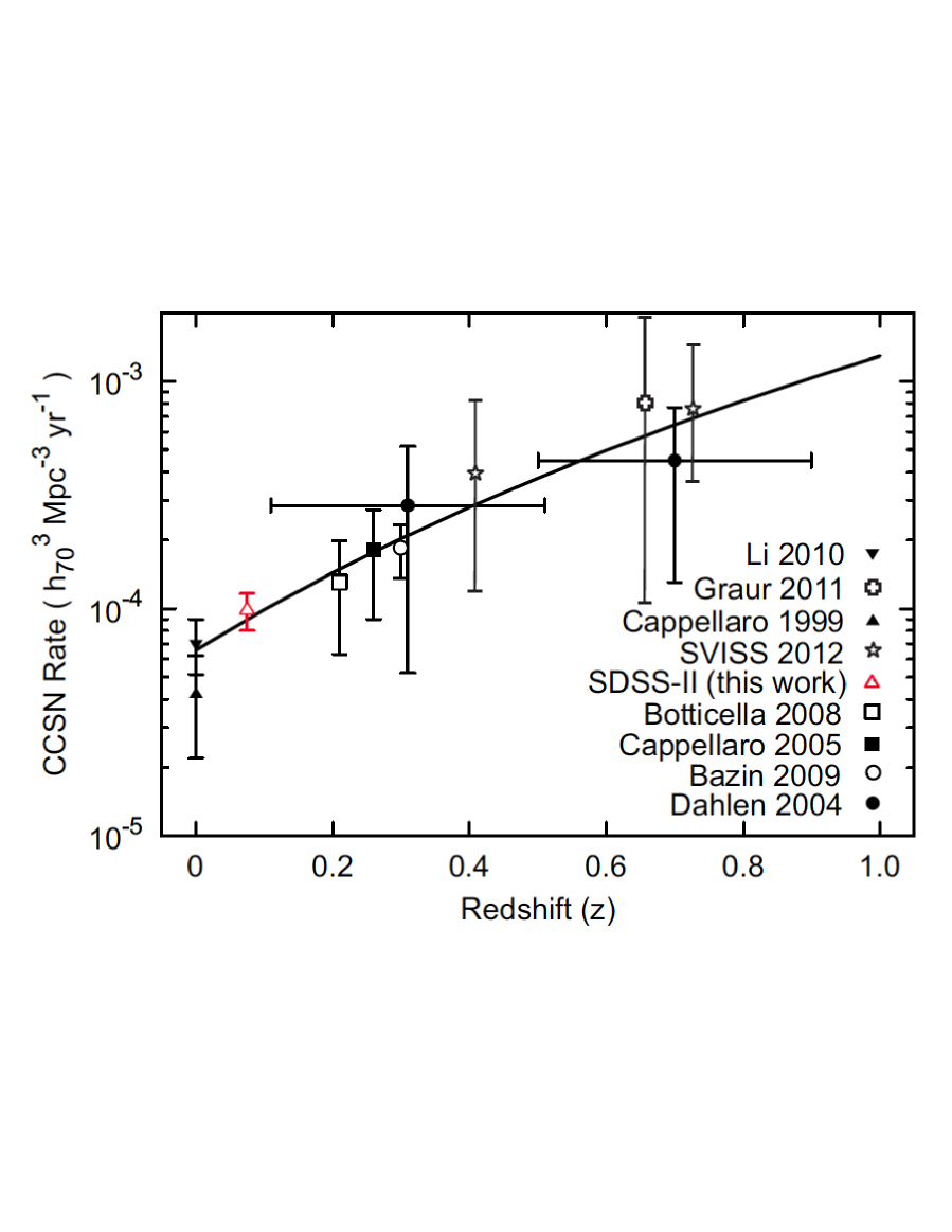
Figure 9: The CCSN rate measurement from this work in red is shown with previous CCSN rate measurements in the literature. The solid line is the star formation rate, scaled to fit the measured CCSN rates.

Our result is generally consistent with the trend identified in earlier CCSN surveys, but provides coverage in a redshift range not previously measured.

We would like to compare the CCSN rate with the star formation rate. Unfortunately establishing exact correspondence between these two rates is complicated by our inability to observe the dimmest CCSNe. This includes both CCSNe that are intrinsically dim, and those that are obscured by dust in the host galaxy. In an effort to better understand this sub-luminous CCSN population, we have attempted to characterize the full distribution of CCSN absolute magnitudes, as much as our data will allow.

Figure 10 shows the efficiency-weighted absolute magnitude distribution of our CCSN rate sample, plus those candidates excluded only because they were too faint, dimmer than $M=-15$, or at redshift below our 0.03 limit. This is related to the core collapse supernova luminosity function, but does not include corrections for the redshift dependence of our data.

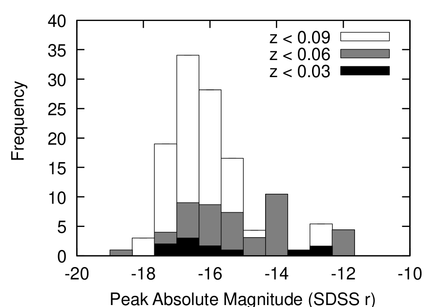
Figure 10: The CCSN luminosity distribution, see text, that we derive for the rate sample in this work, plus candidates excluded only because they were faint or below the redshift range of the rate measure.

The figure suggests that sub-luminous supernovae may be underrepresented in the full rate sample, because a similar number are detected in the small volume lowest redshift and the larger volume mid-redshift bin. To estimate the actual rate of sub-luminous supernovae, we examine the sub-samples for $z<0.03$ and $0.03<z<0.06$. The sub-luminous fractions in these ranges are 20% and 24%, respectively. Our sample is too small to regard these figures as conclusive, but they do suggest that a sub-luminous fraction of 50%, the number required to solve rate problem in Horiuchi (2011), is unlikely. Our data do suggest that there might be a substantial fraction, more than 20%, of sub-luminous supernovae that have been missed in existing rate measurements. This is also suggested in Mattila (2012).

Future surveys promise orders of magnitude increase in the number of supernovae observed. While this will greatly reduce statistical uncertainty, systematic uncertainty may remain comparable to present day surveys, especially because only a small fraction of such events are likely to have spectroscopic redshift measurements. It is possible that almost all galaxy hosts can have their redshifts measured by a massively parallel spectrometer yielding a larger sample of CCSN with secure redshifts which will be important in better measuring the rate of sub-luminous CCSN, a crucial factor in understanding the correspondence between CCSN rate and star formation rate. Also, the increased statistics will be invaluable in more complex supernova measurements, such as understanding the distribution of various supernova characteristics within the CCSN population, and correlating CCSN rate density and characteristics with properties of the host galaxy and location within the galaxy.

9 Conclusion

In conclusion we have measured a bright core collapse supernovae rate density of $(1.06\pm 0.19\times 10^{-4})(h/0.7)^{3}/(\mathrm{Mpc}^{3}\ \mathrm{yr})$ at a mean redshift of $0.072\pm 0.009$. This agrees with the expectation from previous measures and lies along the previously observed trend. Our new result is the most accurate single measurement and is at a newly explored region in redshift. It derives from a sample of 89 light curves observed with the SDSS-II SNS in the redshift range of 0.03 to 0.09 that have been corrected with an efficiency derived from our data and an extinction model from Hatano and collaborators in Hatano (1998).

References

- Bazin (2009) Bazin, G., et al. 2009, A&A, 499, 653
- Bolton (2012) Bolton, A., et al. 2012, AJ, 144, 144
- Botticella (2008) Botticella, M., et al. 2008, A&A, 479, 49
- Botticella (2012) Botticella, M., et al. 2012, A&A, 537, 132
- Campbell (2013) Campbell, H., et al. 2013, ApJ, 763, 88
- Cappellaro (1999) Cappellaro, E., et al. 1999, A&A, 351, 459
- Cappellaro (2005) Cappellaro, E., et al. 2005, A&A, 430, 83
- Cardelli (1989) Cardelli, J., et al. 1989, ApJ, 345, 245
- Cucciati (2012) Cucciati O. et al. 2012 A&A, 539, 31
- Dahlen (2004) Dahlen, T., et al. 2004, ApJ, 613, 189
- Dawson (2013) Dawson, K., et al. 2013, AJ, 145, 10
- Dilday (2008) Dilday, B., et al. 2008, ApJ, 682, 262
- Dilday (2010) Dilday, B., et al. 2010, ApJ, 713, 1026
- Eisenstein (2011) Eisenstein, D. et al. 2011, AJ, 142, 72
- Foley (2013) Foley, Ryan J. et al. 2013, ApJ, 767, 57
- Frieman (2008) Frieman, J., et al. 2008, AJ, 135, 338
- Fukugita (1996) Fukugita, M., et al. 1996, AJ, 111, 1748
- Graur (2011) Graur, O. et al. 2011, MNRAS, 417, 916G
- Gunn (1998) Gunn, J.E., et al. 1998, AJ, 116, 3040
- Gunn (2006) Gunn, J.E., et al. 2006, AJ, 131, 2332
- Hatano (1998) Hatano, K., et al. 1998, ApJ, 502, 177
- Holtzman (2008) Holtzman, J., et al. 2008, AJ, 136, 2306
- Hopkins (2004) Hopkins, A.M. 2004 ApJ, 615, 209-221
- Hopkins&Beacom (2006) Hopkins, A.M. & J. F. Beacom 2006, ApJ, 651, 142-154
- Horiuchi (2011) Horiuchi, S., et al. 2011, ApJ738, 154-159
- Karim (2011) Karim, A., et al. 2011, ApJ730, 61
- Kessler (2009a) Kessler, R., et al. 2009, ApJS, 185, 32
- Kessler (2009b) Kessler, R., et al. 2009, PASP, 121, 1028
- Li (2011) Li, W., et al. 2011, MNRAS, 412, 1441
- Le Floc’h (2005) Le Floc’h E. et al. 2005, ApJ, 632, 169
- Mathews (2014) Mathews, G., et al. arXiv:1405.0458 [astro-ph.CO]
- Mattila (2012) Mattila, S., et al. 2012, ApJ, 756, 111
- Melinder (2012) Melinder, J. et al. 2012, A&A, 545, 96
- Olmstead (2013) Olmstead, M.D. et al. arXiv:1308.6818 [astro-ph.CO]
- Rujopakarn (2010) Rujopakarn W. et al. 2010 ApJ, 718, 1171
- Sako (2008) Sako, M., et al. 2008, AJ, 135, 348
- Sako (2011) Sako, M., et al. 2011, AJ, 738, 162s
- Sako (2014) arXiv:1401.3317 [astro-ph.CO]
- Schiminovich (2005) Schiminovich, D., et al. 2005 ApJ619, L47
- Smee (2013) Smee, S.A., et al. 2013, AJ, in press
- Taylor (2011) Taylor, M., 2011, “The Core Collapse Supernova Rate in the SDSS-II Supernova Survey”, Ph.D. Thesis, Wayne State University
- Vardanyan (2011) Vardanyan, M., iCosmos Cosmology Calculator, Retrieved from http://www.icosmos.co.uk, April 10, 2011.
- York (2000) York, D.G., et al. 2000, AJ, 120, 1579.
- Zheng (2008) Zheng, C., et al. 2008, AJ, 135, 1766