Astrophysical line diagnosis requires non-linear dynamical atomic modeling

Abstract

Line intensities and oscillator strengths for the controversial 3C and 3D astrophysically relevant lines in neonlike Fe¹⁶⁺ ions are calculated. We show that, for strong x-ray sources, the modeling of the spectral lines by a peak with an area proportional to the oscillator strength is not sufficient and non-linear dynamical effects have to be taken into account. Furthermore, a large-scale configuration-interaction calculation of oscillator strengths is performed with the inclusion of higher-order electron-correlation effects. The dynamical effects give a possible resolution of discrepancies of theory and experiment found by recent measurements, which motivates the use of light-matter interaction models also valid for strong light fields in the analysis and interpretation of astrophysical and laboratory spectra.

Astrophysical spectra recorded by space observatories provide the only means to determine the element composition, temperature, density, and velocity of distant celestial objects such as stars, x-ray binaries, black hole accretion discs, or active galactic nuclei Díaz Trigo et al. (2013); Liu et al. (2013); Bernitt et al. (2012); Behar et al. (2001); Xu et al. (2002); Paerels and Kahn (2003); Brown et al. (2001); van Pradijs and Bleeker (1999); Rybicki and Lightman (2004). Such x-ray (or optical) spectra are often composed of a series of peaks associated with a range of elements, ionic charge states, and transitions. Therefore, a large amount of reliable atomic data is needed to disentangle the physical properties of the emitting objects. Such data—transition energies and probabilities, oscillator strengths, collisional and recombination cross sections, etc.—may be obtained from laboratory astrophysics experiments (see e.g. Bernitt et al. (2012); Hahn et al. (2014); Schnorr et al. (2013); Rudolph et al. (2013); Schmidt et al. (2007); Beiersdorfer et al. (2004, 2001); Brown et al. (1998)) or, more economically, from theoretical calculations (see e.g. Bhatia (1992); Cornille et al. (1994); Safronova et al. (2001); Chen (2001)).

The x-ray emission lines of highly charged Fe ions are among the brightest in astrophysical spectra. Within the last decade, several observations were performed with the space laboratories Chandra and XMM-Newton (see e.g. Huenemoerder et al. (2011); Paerels and Kahn (2003); Xu et al. (2002); Mewe et al. (2001)). The line-strength ratio of two $2p\to 3d$ lines in Fe¹⁶⁺, customarily denoted as 3C [$2p^{6}(J=0)\rightarrow(2p^{5})_{1/2}3d_{3/2}\leavevmode\nobreak\ (J=1)$, transition energy of 826 eV] and 3D [$2p^{6}(J=0)\rightarrow(2p^{5})_{3/2}3d_{5/2}\leavevmode\nobreak\ (J=1)$, at 812 eV], was observed, but the results disagreed with theoretical predictions Bhatia (1992); Cornille et al. (1994); Safronova et al. (2001); Chen (2001). Initially this disagreement was considered to originate from the co-existence of different charge states of Fe, and later, after laboratory measurements, as an effect of electron-impact excitation of the ion. Furthermore, since several theoretical calculations of transition probabilities in highly charged ions agreed well with the experiments (see, e.g. Tupitsyn et al. (2005); Volotka et al. (2006); Lapierre et al. (2005)), there was no reason to assume that essential contributions had not been included in the predictions. The question was out of focus until the first laser spectroscopic experiment in the x-ray regime Bernitt et al. (2012), enabled by the advent of x-ray free-electron-laser (XFEL) facilities Emma et al. (2010). This experiment at the Linac Coherent Light Source (LCLS, Ref. LCL ) gave hints for an incorrect atomic structure theory: a disagreement between all state-of-the-art theoretical predictions (ratio of the 3C and 3D oscillator strength around 3.5 and above) and the experimental line-strength ratio of 2.61(23) has been stated Bernitt et al. (2012). In the comparison and in previous astrophysical modeling, it was assumed that the intensity of a line is proportional to the electric dipole oscillator strength.

In this Letter, motivated by the above discrepancy, we refine the theory of x-ray–ion interactions by calculating higher-order electron-correlation and dynamical effects contributing to the 3C/3D line-strength ratio. Our results suggest that the disagreement may be removed by the inclusion of non-linear dynamical effects present in the case of strong driving x-ray fields. The broadening of the spectral lines due to the high x-ray intensity depends on the dipole moment of the transitions involved, significantly influencing both the line strengths as well as their ratio.

Higher-order correlation and QED corrections to the oscillator strengths. To improve the atomic structure theory of the dipole transition rates, we first apply a large-scale implementation of the configuration-interaction Dirac-Fock-Sturm (CI-DFS) method Tupitsyn et al. (2003, 2005), which uses radial wave functions obtained by the numerical solution of the Dirac-Fock equation for the occupied orbitals ($1s$, $2s$, $2p$, $3d$), and virtual orbitals with positive and negative energies represented by a relativistic Sturmian basis set. These orbitals are employed to construct configuration state functions, i.e., Slater determinants $|\Phi^{i}_{J}\rangle$ ($i=1,\dots,N$, where $N$ is the total number of configurations) in an angular momentum-coupled basis with a total angular momentum $J$. The atomic wave function $|\Psi_{J}\rangle$ is finally represented as a linear combination of a large set of configurations:

$$|\Psi_{J}\rangle=\sum_{i=1}^{N}c_{i}|\Phi_{J}^{i}\rangle.$$ (1)

The Einstein coefficients $A_{eg}$ and oscillator strengths $f_{eg}$ are calculated with such wave functions representing the $2p^{6}$ ground $(g)$ and excited $(e\in\{(2p^{5})_{1/2}3d_{3/2},(2p^{5})_{3/2}3d_{5/2}\})$ states of the ion Grant (1974):

$$A_{eg} = \frac{4\pi^{2}e^{2}c^{2}}{(2J_{i}+1)\omega_{eg}}\sum_{M_{i},M_{f}}\sum_{\vec{k}/k,\sigma}\left|\langle{e}|\vec{\alpha}\vec{\epsilon}_{\vec{k}\sigma}e^{-i\vec{k}\vec{r}}|{g}\rangle\right|^{2}\,,$$

$$f_{eg} = \frac{2J_{e}+1}{2J_{g}+1}\frac{A_{eg}mc^{3}}{2\omega^{2}_{eg}e^{2}}\,.$$ (2)

Here, the summation goes over the magnetic quantum numbers of the initial and final states and the polarization $\sigma$ of the emitted photon, and, in addition, an integration is performed over the direction $\vec{k}/k$ of the emitted photon. $c$, $e$ and $m$ denote here the speed of light, the elementary charge, and the electron mass, respectively, and $\vec{\alpha}$ and $\vec{\epsilon}_{\vec{k}\sigma}$ stand for the vector of alpha matrices and the photon polarization unit vector. The dimensionless oscillator strength is of particular interest, as for low driving-field intensities it is proportional to the line strength, here given as the integrated peak area of the resonance photon scattering cross section Grant (1974); Foot (2005):

$$S_{eg}=\frac{\pi^{2}c^{2}\hbar^{3}}{(\hbar\omega)^{2}}\frac{g_{e}}{g_{g}}A_{eg}\propto f_{eg}\,.$$ (3)

In order to match the accuracy of the experimental transition energies $\omega_{eg}=\omega_{e}-\omega_{g}$, additional quantum-electrodynamic (QED) corrections are taken into account in an ab initio manner. The QED corrections in first order in the fine-structure constant $\alpha$ consist of the self-energy (SE) and vacuum-polarization (VP) terms. The SE correction is decomposed into zero-, one-, and many-potential terms. The zero-potential and one-potential terms are calculated in momentum space using formulas from Ref. Yerokhin and Shabaev (1999). The residual part of the SE correction, the so-called many-potential term, is calculated in coordinate space. For any given intermediate-state angular momenta, the summation over the Dirac spectrum is performed using the dual-kinetic-balance approach Shabaev et al. (2004) with basis functions constructed from B-splines. The VP correction was calculated in the Uehling approximation Uehling (1935). Electron-interaction contributions to the QED corrections were calculated by evaluating the single-electron QED diagrams with an effective potential accounting for the screening of the remaining 9 electrons, as described in Ref. Schnorr et al. (2013). We find that although screening effects significantly modify the single-electron QED corrections, the total QED effect on the transition energies is on the 10-meV level.

While we can conclude that transition energies entering the theoretical oscillator strengths can be predicted with sufficient accuracy, the discrepancy with the measurements prevails, and it may be rooted in the calculation of the non-diagonal dipole matrix elements. In all previous theoretical studies it was assumed that the correlated many-electron wave function can be well represented by constructing the configuration space with single and double electron exchanges from the reference-state configuration. Here we also take into account triple excitations, resulting in a huge number of configurations. As a result, for the case of single and double excitations included, the 3C/3D oscillator strength ratio is 3.57, while the contribution of the triple excitation is as low as -0.01. Thus, our results confirm earlier theoretical calculations and disprove the significance of triple excitations, suggesting that the discrepancy of theory and experiment is not funded in the inaccurate description of the ions’ electronic structure.

Modeling of strong-field effects. Once insufficiencies in structure calculations are ruled out, the next to investigate are dynamical aspects of light-matter interaction. In Ref. Bernitt et al. (2012) and in previous studies it was implicitly assumed that the intensity of the observed lines is proportional to the oscillator strength. This holds true under the assumption of a relatively weak exciting field. However, nonlinearities are anticipated if the intensity $I$ of the field is comparable to or larger than the saturation intensity $I_{\rm sat}$, to be defined below. For the Fe transitions studied, with $I_{\rm sat}\approx$ $10^{11}$ W/cm², the intensity of LCLS pulses is typically on or above this order of magnitude, such that the exciting field cannot be considered as weak anymore.

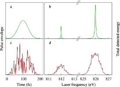
Figure 1: (a) Time-envelope of a Gaussian and (c) an incoherent pulse, in arbitrary units. (b,d) The fluorescence signal (total energy of fluorescence photons) as a function of the XFEL photon energy in the energy range of the 3C and 3D transitions in Fe¹⁶⁺, in arbitrary units. Here, an x-ray intensity of $I=10^{13}$ W/cm² was used and results are shown for (c) a Gaussian pulse and (d) after averaging over 10 incoherent pulses with a time duration of $T=200$ fs. For incoherent pulses, the bandwidth is set to $B=1$ eV.

We therefore improve the physical description and perform time-dependent simulations by modeling the ion as a two-level system with ground state $|g\rangle$ and excited state $|e\rangle$. The transition energy $\omega_{eg}$ approximately equals 826 eV and 812 eV for the 3C and 3D lines, respectively, and the decay width is $\Gamma_{eg}=\hbar A_{eg}$. We describe the atomic system via the density matrix $\hat{\rho}(t)$ of elements $\rho_{ij}$, with $i,\,j\in\{g,\,e\}$, whose evolution in time is given by the master equation Scully and Zubairy (1997); Kiffner et al. (2010)

$$\frac{d\hat{\rho}}{dt}=-\frac{i}{\hbar}[\hat{H},\hat{\rho}(t)]+L\hat{\rho}(t)\,,$$ (4)

where the square brackets stand for a commutator, and the Lindblad superoperator $L$ represents the spontaneous decay from the exited state $|e\rangle$ to the ground state $|g\rangle$ with decay rates equal to $2.22\times 10^{13}$ s^-1 and $6.02\times 10^{12}$ s^-1 for the 3C and the 3D transitions, respectively, according to our CI-DFS calculations. The Hamiltonian $\hat{H}=\hat{H}_{0}+\hat{H}_{\mathrm{int}}$ is the sum of the electronic-structure Hamiltonian $\hat{H}_{0}=\sum_{i\in\{g,e\}}\hbar\omega_{i}|i\rangle\langle i|$ and of the Hamiltonian $\hat{H}_{\mathrm{int}}$ describing the interaction of the ion with an external time-dependent electric field $\mathcal{E}(t)=E(t)\,\cos(\omega_{\mathrm{X}}t+\psi(t))$ of x-ray carrier frequency $\omega_{\mathrm{X}}$, envelope $E(t)$, and phase $\psi(t)$. We introduce the vector $\vec{R}(t)$ of the slowly varying components of the density matrix,

$$\vec{R}(t)=(\rho_{gg}(t),\,\rho_{ge}(t)\,e^{-i\omega_{\mathrm{X}}t},\,\rho_{eg}(t)\,e^{i\omega_{\mathrm{X}}t},\,\rho_{ee}(t))^{\mathrm{T}}\,,$$ (5)

such that the master equation can be written in the matrix form

$$\frac{d\vec{R}(t)}{dt}={\bf M}(t)\vec{R}(t)\,,$$ (6)

with the $4\times 4$ time-dependent matrix

$${\bf M}(t)=\left(\begin{array}[]{c c c c}0&-i\frac{\Omega^{*}_{R}(t)}{2}&i\frac{\Omega_{R}(t)}{2}&\Gamma_{eg}\\ -i\frac{\Omega_{R}(t)}{2}&i\Delta-\frac{\Gamma_{eg}}{2}&0&i\frac{\Omega_{R}(t)}{2}\\ i\frac{\Omega^{*}_{R}(t)}{2}&0&-i\Delta-\frac{\Gamma_{eg}}{2}&-i\frac{\Omega^{*}_{R}(t)}{2}\\ 0&i\frac{\Omega^{*}_{R}(t)}{2}&-i\frac{\Omega_{R}(t)}{2}&-\Gamma_{eg}\\ \end{array}\right)\,.$$

The complex time-dependent Rabi frequency $\Omega_{R}(t)=eE(t)\langle g|\hat{r}|e\rangle e^{i\psi(t)}/\hbar$ is proportional to the square root of the x-ray intensity $I$ and $\Delta=\omega_{eg}-\omega_{X}$ denotes the detuning of the laser frequency from the transition frequency. For a continuous-wave driving field, $E(t)=\bar{E}$, $\psi(t)=0$, with correspondingly constant Rabi frequency $\bar{\Omega}_{R}$, the solution of the master equation (6) converges for $t\rightarrow\infty$ to the stationary solution Scully and Zubairy (1997); Foot (2005)

$$\bar{R}_{ee}(\Delta)=\frac{\bar{\Omega}_{R}^{2}}{4\Delta^{2}+\Gamma_{eg}^{2}+2\bar{\Omega}_{R}^{2}}\,.$$ (8)

The energy detected per unit time for a given detuning $\Delta$ is

$$\mathcal{I}(\Delta)\propto\Gamma_{eg}\omega_{eg}\bar{R}_{ee}(\Delta)\,,$$ (9)

which can be used to calculate the ratio of the intensities emitted by the two lines by means of the integrals over the detuning $\Delta$

$$S_{\rm 3C}/S_{\rm 3D}=\frac{\int{\rm d}\Delta\mathcal{I}_{\rm 3C}(\Delta)}{\int{\rm d}\Delta\mathcal{I}_{\rm 3D}(\Delta)}\,.$$ (10)

By introducing for each line the saturation intensity $I_{\mathrm{sat}}=I\,\Gamma_{eg}^{2}/(2\bar{\Omega}^{2}_{R})$, this leads to

$$S_{\rm 3C}/S_{\rm 3D}=\frac{\Gamma_{\mathrm{3C}}\omega_{\mathrm{3D}}^{2}}{\Gamma_{\mathrm{3D}}\omega_{\mathrm{3C}}^{2}}\,\sqrt{\frac{1+I/I_{\rm sat,3D}}{1+I/I_{\rm sat,3C}}}.$$ (11)

For a weak exciting field ($I\ll I_{\rm sat}$), this agrees with the linear theory of resonance fluorescence predicting a ratio of 3.56, while in the strong-field limit ($I\gg I_{\rm sat}$) Eq. (11) converges to the value $S_{\rm 3C}/S_{\rm 3D}\rightarrow 7.03$.

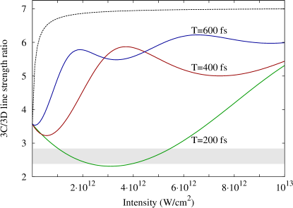
Figure 2: The line-strength ratio $S_{\rm 3C}/S_{\rm 3D}$ as a function of the intensity and duration of the Gaussian pulse. The dashed line is for a continuous wave field (Eq. 10). The gray shaded area shows the experimental ratio 2.61(23) Bernitt et al. (2012) together with its error bar.

For a time-dependent (pulsed) driving field, the system of differential equations (6) is solved assuming the initial conditions $\vec{R}_{0}=(1,0,0,0)^{T}$. Thereby, we can calculate the total detected energy as a function of the detuning,

$$\mathcal{E}(\Delta)\propto\Gamma_{R}\omega_{eg}\int_{-\infty}^{+\infty}R_{ee}(t)dt\,,$$ (12)

where $R_{ee}(t)$ also depends on $\Delta$. This yields a spectrum which can be compared to the experimentally measured one. The ratio of total emitted line energies can be again calculated as a ratio of the integrals over the detuning $\Delta$:

$$S_{\rm 3C}/S_{\rm 3D}=\frac{\int{\rm d}\Delta\mathcal{E}_{\rm 3C}(\Delta)}{\int{\rm d}\Delta\mathcal{E}_{\rm 3D}(\Delta)}\,.$$ (13)

Typical LCLS intensities are in the range of $I=10^{11}-10^{14}$ W/cm² and pulse durations in the range $T=200-2000$ fs. Also, not the total electromagnetic energy emitted in all directions was detected in the experiment Bernitt et al. (2012), but only a fraction of it emitted into a given solid angle. However, since the excited states have the same symmetry (total angular momentum $J=1$) and the ground state of the ion is spherically symmetric ($J=0$), the angular distribution of the emitted radiation is the same for both transitions, allowing one to compare the strength ratio as defined above with the experimentally determined line intensities.

Matching the experimental line strengths and discussion. In Fig. 1b, simulated 3C and 3D fluorescence lines are presented assuming strong XFEL pulses of Gaussian shape for an intensity of $I=10^{13}$ W/cm² and duration of $T=200$ fs. We use the pulse envelope $E(t)=E_{\rm max}e^{-\frac{t^{2}}{T^{2}}32\ln(2)}$ and a constant phase $\psi(t)=0$. The ratio of the 3C and 3D line strengths is shown separately on Fig. 2 as a function of pulse parameters. The strengths and their ratio are sensitive to the change of pulse intensity and duration. Between $I=1-6\times 10^{12}$ W/cm² and for $T=200$ fs, the resulting line-strength ratio is in the range of $2.31-3.08$, as presented in Fig. 2. This result is still in agreement with the measured value of 2.61$\pm$0.23. We also infer that the pulse-by-pulse variation of intensity and duration contributes to the experimental uncertainty of the ratio. These results confirm the importance of strong-field dynamical effects in a relatively intense XFEL field. We note that, in this range of parameters, we are still in the weakly nonlinear regime: below intensities of approximately 10¹¹ W/cm², the linear theory of resonance fluorescence may be applied. (The linear model is also applicable for transitions with significantly lower dipole matrix elements, even if the intensity of the x-ray source is high.) At higher intensities, or for longer pulses, which is also still in the range of possible experimental parameters, the sensitivity to the pulse parameters increases, resulting in an oscillation of the line-strength ratio of the 3C and 3D lines between 5.5 and 6.5, in agreement with the previously mentioned intensity-saturation effects. Increasing the pulse duration in the simulations, one reaches the limit of continuous-wave fields, which is shown by the dashed line [cf. Eq. (10)].

For an even more realistic modeling, we additionally take into account the chaotic nature of XFEL pulses generated via self-amplified spontaneous emission Bonifacio et al. (1984), by modeling amplitude $E(t)$ and phase $\psi(t)$ via the partial-coherence method from Refs. Pfeifer et al. (2010); Cavaletto et al. (2012). An understanding of incoherence effects is not only relevant for laboratory measurements but also for astrophysical observations, as natural x-ray sources lack coherence. In the simulations, we employ a series of such randomized pulses, an example of which is shown on Fig. 1c. Fig. 1d presents the fluorescence signal resulting from the use of such incoherent pulses, while Fig. 3 displays the line-strength ratio (13) obtained with chaotic pulses of different duration, intensity and bandwidth. Each point in Fig. 3 is obtained by averaging over 10 independent realizations of a chaotic pulse. The numerical uncertainty of the obtained results is estimated to be on the level of $1-2\%$. As in the case of Gaussian pulses, the line-strength ratio clearly depends on the pulse parameters. Also here, for small intensities, the value of 3.56 is approached, in agreement with the linear theory of resonance fluorescence. We notice that, for incoherent pulses, the effect of the decrease in the 3C/3D line-strength ratio can be observed within a wider range of pulse intensities than for Gaussian pulses, as well as for a significantly larger interval of pulse durations. As shown in the picture, this effect becomes more significant at increasing values of the bandwidth (i.e., the FWHM of the energy spectrum) of the chaotic pulse, which in the experiment Bernitt et al. (2012) can be estimated to be of the order of 1 eV. The decrease in bandwidth (increase in coherence time) corresponds to a more coherent pulse, and a behaviour closer to that displayed by fully coherent (transform-limited) Gaussian pulses.

Although parameters of XFEL pulses are not fixed from pulse to pulse because of their chaotic nature, the average peak intensity may be estimated to lie in the considered range. However, the predicted decrease in the 3C/3D ratio within a broad interval of pulse intensities and pulse durations allow us to suggest that the observed unexpectedly low value of the 3C/3D ratio is determined by previously neglected nonlinear dynamical effects.

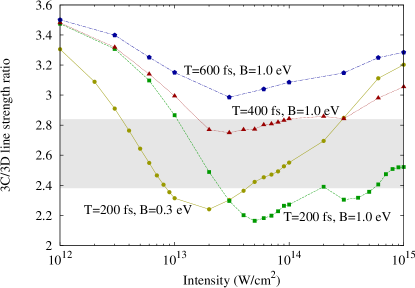
Figure 3: The line-strength ratio $S_{\rm 3C}/S_{\rm 3D}$ as a function of the intensity $I$ and duration $T$ of the incoherent pulse. For the shortest pulses, results with two different bandwidths $B$ are shown. The gray shaded area shows the experimental ratio 2.61(23) Bernitt et al. (2012) together with its error bar.

In summary, we conclude that a new approach is called for in astrophysical line diagnostics, taking into account effects depending on the intensity of the radiation field. Above certain intensities, weak-field atomic theory may not give a proper picture of radiative processes taking place in, e.g., black hole accretion discs. For stellar-mass black holes, the Eddington luminosity of approx. $10^{38}$ erg/s translates to a total radiation intensity (integrated over the Planck distribution at a temperature of $5\times 10^{7}$ K Shapiro and Teukolsky (1983)) on the order of $10^{18}$ W/cm² at a distance of 3 Schwarzschild radii, of which approximately $3\times 10^{13}$ W/cm² is in a typical 1-eV range of an atomic line at 1 keV. Furthermore, such nonlinear dynamic effects also have to be considered in laboratory astrophysics experiments employing sources of high x-ray intensities, such as, e.g., x-ray free-electron lasers.

We acknowledge helpful advice from Ilya I. Tupitsyn and insightful conversations with Alberto Benedetti.

References

- Díaz Trigo et al. (2013) M. Díaz Trigo, J. C. A. Miller-Jones, S. Migliari, J. W. Broderick, and T. Tzioumis, Nature 504, 260 (2013).
- Liu et al. (2013) J.-F. Liu, J. N. Bregman, Y. Bai, S. Justham, and P. Crowther, Nature 503, 500 (2013).
- Bernitt et al. (2012) S. Bernitt, G. V. Brown, J. K. Rudolph, R. Steinbrügge, A. Graf, M. Leutenegger, S. W. Epp, S. Eberle, K. Kubiček, V. Mäckel, M. C. Simon, E. Träbert, E. W. Magee, C. Beilmann, N. Hell, S. Schippers, A. Müller, S. M. Kahn, A. Surzhykov, Z. Harman, C. H. Keitel, J. Clementson, F. S. Porter, W. Schlotter, J. J. Turner, J. Ullrich, P. Beiersdorfer, and J. R. Crespo López-Urrutia, Nature 492, 225 (2012).
- Behar et al. (2001) E. Behar, J. Cottam, and S. M. Kahn, Astrophys. J. 548, 966 (2001).
- Xu et al. (2002) H. Xu, S. M. Kahn, J. R. Peterson, E. Behar, F. B. S. Paerels, R. F. Mushotzky, J. G. Jernigan, A. C. Brinkman, and K. Makishima, Astrophys. J. 579, 600 (2002).
- Paerels and Kahn (2003) F. B. S. Paerels and S. M. Kahn, Annu. Rev. Astron. Astrophys. 41, 291 (2003).
- Brown et al. (2001) G. V. Brown, P. Beiersdorfer, H. Chen, M. H. Chen, and K. J. Reed, Astrophys. J. 557, L75 (2001).
- van Pradijs and Bleeker (1999) J. van Pradijs and J. A. M. Bleeker, eds., X-ray spectroscopy in astrophysics (Springer-Verlag, 1999).
- Rybicki and Lightman (2004) G. B. Rybicki and A. P. Lightman, Radiative processes in astrophysics (John Wiley & Sons, 2004).
- Hahn et al. (2014) M. Hahn, N. R. Badnell, M. Grieser, C. Krantz, M. Lestinsky, A. Müller, O. Novotný, R. Repnow, S. Schippers, A. Wolf, and D. W. Savin, Astrophys. J. 788, 46 (2014).
- Schnorr et al. (2013) K. Schnorr, V. Mäckel, N. S. Oreshkina, S. Augustin, F. Brunner, Z. Harman, C. H. Keitel, J. Ullrich, and J. R. Crespo López-Urrutia, Astrophys. J. 776, 121 (2013).
- Rudolph et al. (2013) J. K. Rudolph, S. Bernitt, S. W. Epp, R. Steinbrügge, C. Beilmann, G. V. Brown, S. Eberle, A. Graf, Z. Harman, N. Hell, M. Leutenegger, A. Müller, K. Schlage, H.-C. Wille, H. Yavaş, J. Ullrich, and J. R. Crespo López-Urrutia, Phys. Rev. Lett. 111, 103002 (2013).
- Schmidt et al. (2007) E. W. Schmidt, D. Bernhardt, A. Müller, S. Schippers, S. Fritzsche, J. Hoffmann, A. S. Jaroshevich, C. Krantz, M. Lestinsky, D. A. Orlov, A. Wolf, D. Lukić, and D. W. Savin, Phys. Rev. A 76, 032717 (2007).
- Beiersdorfer et al. (2004) P. Beiersdorfer, M. Bitter, S. von Goeler, and K. W. Hill, Astrophys. J. 610, 616 (2004).
- Beiersdorfer et al. (2001) P. Beiersdorfer, S. von Goeler, M. Bitter, and D. B. Thorn, Phys. Rev. A 64, 032705 (2001).
- Brown et al. (1998) G. V. Brown, P. Beiersdorfer, D. A. Liedahl, K. Widmann, and S. M. Kahn, Astrophys. J. 502, 1015 (1998).
- Bhatia (1992) A. K. Bhatia, At. Data and Nucl. Data Tables 52, 1 (1992).
- Cornille et al. (1994) M. Cornille, J. Dubau, and S. Jacquemot, At. Data and Nucl. Data Tables 58, 1 (1994).
- Safronova et al. (2001) U. I. Safronova, C. Namba, I. Murakami, W. R. Johnson, and M. S. Safronova, Phys. Rev. A 64, 012507 (2001).
- Chen (2001) G.-X. Chen, Phys. Rev. A 76, 062708 (2001).
- Huenemoerder et al. (2011) D. P. Huenemoerder, A. Mitschang, D. Dewey, M. A. Nowak, N. S. Schulz, J. S. Nichols, J. E. Davis, J. C. Houck, H. L. Marshall, M. S. Noble, D. Morgan, and C. R. Canizares, Astron. J. 141, 129 (2011).
- Mewe et al. (2001) R. Mewe, A. J. J. Raassen, J. J. Drake, J. S. Kaastra, R. L. J. van der Meer, and D. Porquet, Astron. Astrophys. 368, 888 (2001).
- Tupitsyn et al. (2005) I. I. Tupitsyn, A. V. Volotka, D. A. Glazov, V. M. Shabaev, G. Plunien, J. R. Crespo López-Urrutia, A. Lapierre, and J. Ullrich, Phys. Rev. A 72, 062503 (2005).
- Volotka et al. (2006) A. V. Volotka, D. A. Glazov, G. Plunien, V. M. Shabaev, and I. I. Tupitsyn, Eur. Phys. J. D 38, 293 (2006).
- Lapierre et al. (2005) A. Lapierre, U. D. Jentschura, J. R. Crespo López–Urrutia, J. Braun, G. Brenner, H. Bruhns, D. Fischer, A. J. González Martínez, Z. Harman, W. R. Johnson, C. H. Keitel, V. Mironov, C. J. Osborne, G. Sikler, R. S. Orts, V. Shabaev, H. Tawara, I. I. Tupitsyn, J. Ullrich, and A. Volotka, Phys. Rev. Lett. 95, 183001 (2005).
- Emma et al. (2010) P. Emma, R. Akre, J. Arthur, R. Bionta, C. Bostedt, J. Bozek, A. Brachmann, P. Bucksbaum, R. Coffee, F.-J. Decker, Y. Ding, D. Dowell, S. Edstrom, A. Fisher, J. Frisch, S. Gilevich, J. Hastings, G. Hays, P. Hering, Z. Huang, R. Iverson, H. Loos, M. Messerschmidt, A. Miahnahri, S. Moeller, H.-D. Nuhn, G. Pile, D. Ratner, J. Rzepiela, D. Schultz, T. Smith, P. Stefan, H. Tompkins, J. Turner, J. Welch, W. White, J. Wu, G. Yocky, and J. Galayda, Nature Photon. 4, 641 (2010).
- (27) “Linac Coherent Light Source,” http://lcls.slac.stanford.edu.
- Tupitsyn et al. (2003) I. I. Tupitsyn, V. M. Shabaev, J. R. Crespo López-Urrutia, I. Draganić, R. Soria Orts, and J. Ullrich, Phys. Rev. A 68, 022511 (2003).
- Grant (1974) I. P. Grant, J. Phys. B 7, 1458 (1974).
- Foot (2005) C. J. Foot, Atomic Physics (Oxford University Press, 2005).
- Yerokhin and Shabaev (1999) V. Yerokhin and V. M. Shabaev, Pys. Rev. A 60, 800 (1999).
- Shabaev et al. (2004) V. M. Shabaev, I. I. Tupitsyn, V. A. Yerokhin, G. Plunien, and G. Soff, Phys. Rev. Lett 93, 130405 (2004).
- Uehling (1935) E. A. Uehling, Phys. Rev. 48, 55 (1935).
- Scully and Zubairy (1997) M. O. Scully and S. Zubairy, Quantum Optics (Cambrige University Press, Cambridge, 1997).
- Kiffner et al. (2010) M. Kiffner, M. Macovei, J. Evers, and C. H. Keitel, in Prog. Opt., Vol. 55, edited by E. Wolf (Elsevier, 2010) Chap. 3, p. 85.
- Bonifacio et al. (1984) R. Bonifacio, C. Pellegrini, and L. Narducci, Optics Communications 50, 373 (1984).
- Pfeifer et al. (2010) T. Pfeifer, Y. Jiang, S. Düsterer, R. Moshammer, and J. Ullrich, Opt. Lett. 35, 3441 (2010).
- Cavaletto et al. (2012) S. M. Cavaletto, C. Buth, Z. Harman, E. P. Kanter, S. H. Southworth, L. Young, and C. H. Keitel, Phys. Rev. A 86, 033402 (2012).
- Shapiro and Teukolsky (1983) S. L. Shapiro and S. A. Teukolsky, Black holes, white dwarfs and neutron stars: the physics of compact objects (John Wiley & Sons, 1983).