Numerical stability analysis of the Euler scheme for BSDEs

Abstract.

In this paper, we study the qualitative behaviour of approximation schemes for Backward Stochastic Differential Equations (BSDEs) by introducing a new notion of numerical stability. For the Euler scheme, we provide sufficient conditions in the one-dimensional and multidimensional case to guarantee the numerical stability. We then perform a classical Von Neumann stability analysis in the case of a linear driver $f$ and exhibit necessary conditions to get stability in this case. Finally, we illustrate our results with numerical applications.

Key words: BSDEs, Approximation, Numerical stability.

MSC Classification (2000): 93E20, 65C99, 60H30.

1. Introduction

In this paper, we study the qualitative behaviour of a class of numerical methods for Backward Stochastic Differential Equations (BSDEs) by introducing a new notion of numerical stability. Even though we will focus exclusively on the numerical schemes, we recall, to motivate our work the definition of BSDEs in a classical setting, see e.g. [25]. Let $(\Omega,\mathcal{A},\mathbb{P})$ be a probability space supporting a $d$-dimensional Brownian motion $(W_{t})_{t\geq 0}$. We denote by $\mathbb{F}:=(\mathcal{F}_{t})_{t\geq 0}$ the Brownian filtration. Let $T>0$, $\xi$ be an $\mathcal{F}_{T}$-measurable and square-integrable random variable and $f:\Omega\times\mathbb{R}^{+}\times\mathbb{R}^{d}\times\mathbb{R}^{m\times d}\rightarrow\mathbb{R}^{m}$ in such a way that the process $(f(t,y,z))_{t\in[0,T]}$ is progressively measurable for all $(y,z)\in\mathbb{R}^{m}\times\mathbb{R}^{m\times d}$ and $\mathbb{E}\left[\int_{0}^{T}\left|f(s,0,0)\right|^{2}ds\right]<+\infty$. The solution $(\mathcal{Y},\mathcal{Z})$ of a BSDEs satisfies

$$\mathcal{Y}_{t}=\xi+\int_{t}^{T}f(s,\mathcal{Y}_{s},\mathcal{Z}_{s})\mathrm{d}s-\int_{t}^{T}\mathcal{Z}_{s}\mathrm{d}W_{s}\;.$$ (1.1)

If we assume that $f$ is a Lipschitz function with respect to $y$ and $z$ then it is known [25] that the BSDE (1.1) has a unique solution $(\mathcal{Y},\mathcal{Z})\in\mathscr{S}^{2}\times\mathscr{H}^{2}$ where $\mathscr{S}^{2}$ is the set of continuous adapted processes satisfying $\mathbb{E}\!\!\left[\sup_{s\in[0,T]}|U_{s}|^{2}\right]<\infty$ and $\mathscr{H}^{2}$ is the set of progressively measurable processes $V$ satisfying $\mathbb{E}\!\!\left[\int_{0}^{T}|V_{t}|^{2}\mathrm{d}t\right]<\infty$. Let us mention also that it is possible to relax some assumptions on $f$ and $\xi$: see e.g. [23] for monotone generators with respect to $y$, [3] for $L^{p}$ solutions and [19] for quadratic generators with respect to $z$. These equations have applications e.g. in PDE analysis through non-linear Feynman-Kac formula [24, 14], stochastic control theory [22] or mathematical finance [17]. Recently, they have been used as non linear pricing methods [12, 13, 7, 6]. In the past ten years, a lot of work has also been done on the numerical approximation of the above BSDE (and extensions) see e.g. [28, 2, 18, 9] and the references therein, especially in a markovian setting. This means that the terminal condition and the random part of the generator are given by deterministic measurable functions of a forward diffusion $X$, precisely $\xi:=g(X_{T})$ and $f(t,y,z)=\bar{f}(t,X_{t},y,z)$, with

$$X_{t}=X_{0}+\int_{0}^{t}b(X_{s})\mathrm{d}s+\int_{0}^{t}\sigma(X_{s})\mathrm{d}W_{s}\;,\;t\in[0,T]\,.$$

Here, we assume that $g$, $x\mapsto\bar{f}(t,x,y,z)$, $b$ and $\sigma$ are Lipschitz-continuous function.

One of the first numerical method that has been proposed, see e.g. [28, 2] and the references therein for early works, is given by a discrete backward programming equation. Given a grid $\pi=\{t_{0}:=0,\dots,t_{i},\dots,t_{n}:=T\}$, one sets $Y_{n}=\xi$ and compute at each step:

$$Y_{i} =\mathbb{E}_{t_{i}}\!\!\left[Y_{i+1}+(t_{i+1}-t_{i})f(t_{i},Y_{i},Z_{i})\right]$$ (1.2)

$$Z_{i} =\mathbb{E}_{t_{i}}\!\!\left[\frac{1}{t_{i+1}-t_{i}}Y_{i+1}(\Delta W_{i})^{\prime}\right]$$ (1.3)

where $\Delta W_{i}:=W_{t_{i+1}}-W_{t_{i}}$, $\mathbb{E}_{t}\!\!\left[\cdot\right]$ stands for $\mathbb{E}\!\!\left[\cdot\,|\,\mathcal{F}_{t}\right]$ and ^′ denotes the transpose operator.

The above scheme is implicit in $Y$ and one can compute alternatively

$$Y_{i}=\mathbb{E}_{t_{i}}\!\!\left[Y_{i+1}+(t_{i+1}-t_{i})f(t_{i},Y_{i+1},Z_{i})\right]$$ (1.4)

to get an explicit version.

It has been shown that, in the Lipschitz setting, the above method has order at least one-half [28, 2] and generally at most one [18, 10]. Recently, other methods have been proposed with high order of convergence, one step methods as Runge-Kutta method [10] and linear multi-step method [9]. A first motivation for this work comes from the need to distinguish between ’good’ and ’bad’ methods provided by the above papers. Indeed, the order of convergence of a scheme is an asymptotic property that allows to classify schemes when the number of time-steps tends to infinity. We would like here to know the quality of a scheme when the number of timesteps is set.

The study we perform in this paper can be seen as an extension of the numerical stability study of numerical schemes for ODEs, in the context of BSDEs. Indeed, if one considers a deterministic terminal value for $\xi$ and a deterministic generator $f$, in the one-dimensional setting the BSDE reduces to an ODE, and the corresponding scheme to an Euler method for ODE. It is well known, see e.g. [8], that implicit and explicit Euler method have different stability behaviour in practice when $f$ is monotone. In particular, the explicit Euler method may become unstable if the timestep $h$ is not small enough. One should expect this behaviour also for the above BSDE scheme. The framework of BSDEs is (in some sense) richer than the one for ODEs and studying the stability of the methods given in (1.2)-(1.3) or (1.4)-(1.3) is already a challenging task. Moreover, to the best of our knowledge, it is the first time that such a study is undertaken. In the next paragraph, we motivate our work with an example belonging ’purely’ to the BSDEs framework.

1.1. A motivating example

Let us consider the BSDE (1.1) with the following choice of coefficients: $g(\cdot)=\cos(\alpha\cdot)$, $X=W$ (dimension one) and $f(t,y,z)=bz$, for given real numbers $\alpha$ and $b$. Namely, $(\mathcal{Y},\mathcal{Z})$ is solution to,

$$\mathcal{Y}_{t}=cos(\alpha W_{T})+\int_{t}^{T}b\mathcal{Z}_{s}\mathrm{d}s-\int_{t}^{T}\mathcal{Z}_{s}\mathrm{d}W_{s}\;,t\leq T\;.$$ (1.5)

At time $t=0$, the $\mathcal{Y}$ component is easily computed and given by

$$\mathcal{Y}_{0}=e^{-\alpha^{2}\frac{T}{2}}\cos(\alpha bT)\;.$$

We observe that $\mathcal{Y}_{0}$ is bounded by $1$, the bound of the terminal condition and moreover, $\mathcal{Y}_{0}\rightarrow 0$ as $T\rightarrow\infty$. This can be interpreted as a stability property of the BSDE, see next section, Proposition 1.1 .

We then consider the numerical approximation introduced in (1.2)-(1.3) above. In order to compute the conditional expectations and set the terminal value, we simply use a trinomial (recombining) tree for the Brownian motion, see e.g. [9] and an equidistant time grid of $[0,T]$ with $h=\frac{T}{n}$ and $n+1$ time steps. It is well known that, in this context, the error for the $\mathcal{Y}$ part is given by $\mathcal{Y}_{0}-Y_{0}=O(h),$ where $Y_{0}$ is the solution at time $0$ returned by the scheme, see [18, 9]. Let us now try to observe this behaviour in practice by plotting the error $|\mathcal{Y}_{0}-{Y}_{0}|$ against the number of step, in logarithmic scale, for different value of $(b,T)$, $\alpha$ being set to $1$.

Figure 1. Euler Scheme, $(b=1,T=10)$

Figure 2. Euler Scheme, $(b=5,T=1)$

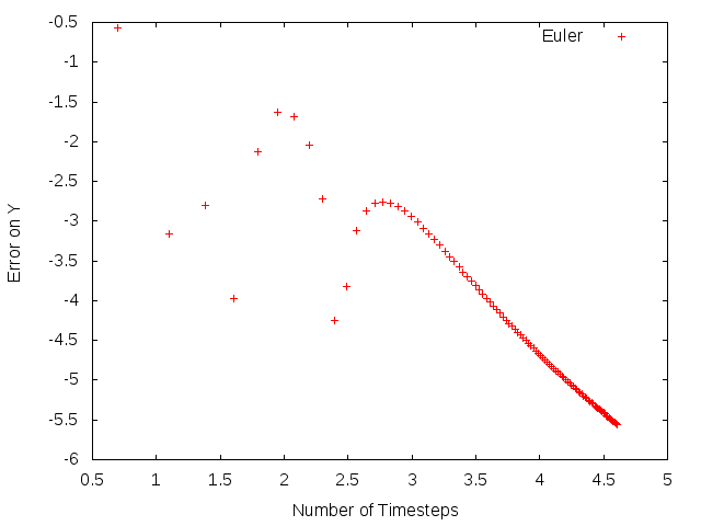
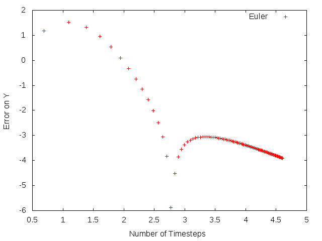
On Figure 1 and 2 appears clearly a first transient state and then the asymptotic steady state, after a number of time step (between $25$ and $35$). This means that the linear convergence is obtained for $h$ being smaller that some $h^{*}$. This phenomenon appears here if $b$ is ’big’ or $T$ is ’big’. On Figure 3, where both $b$ and $T$ are ’big’, things are even worse. The correct behaviour of the scheme is observed only for very large $n$ ($n$ is larger than $240$).

Figure 3. Euler Scheme, $(b=5,T=10)$

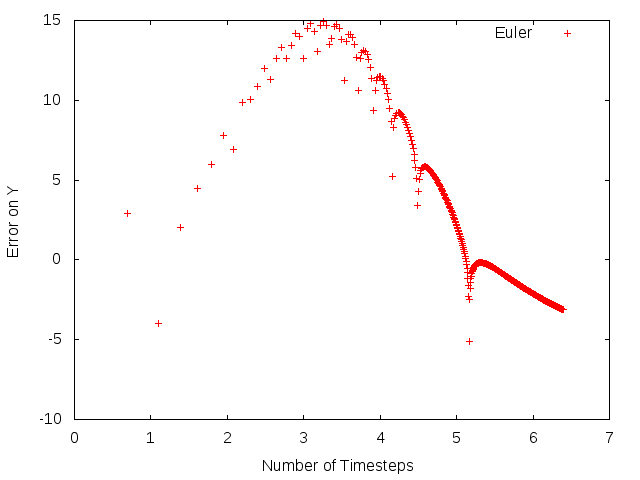
We see that even in the ’pure’ BSDE setting, i.e. when $f$ depends only on $z$, the numerical method exhibits some instability. In the sequel, we investigate this unstable behaviour and provide sufficient and necessary (in some sense) conditions in order to avoid it.

1.2. Main assumptions and stability of BSDEs

Before stating a precise definition of numerical stability, we recall some known sufficient conditions to obtain a bounded solution $\mathcal{Y}$ to (1.1). Since we are interested in the numerical behavior of discretization schemes for BSDEs, we simplify our framework by assuming that the generator is deterministic and does not depend on time $t$ (denoted $(y,z)\mapsto f(y,z)$ by an abuse of notation). We also suppose that $f(0,0)=0$.

In the sequel, we shall make use of the following assumptions.

$({HfLy})$: The function $f$ is Lipschitz continuous with respect to $y$ with Lipschitz constant $L^{Y}\geq 0$, i.e.

$$|f(y^{\prime},z)-f(y,z)|\leq L^{Y}|y-y^{\prime}|.$$

$({HfLz})$: The function $f$ is Lipschitz continuous with respect to $z$ with Lipschitz constant $L^{Z}\geq 0$, i.e.

$$|f(y,z^{\prime})-f(y,z)|\leq L^{Z}|z-z^{\prime}|.$$

$({Hfmy})$: The function $f$ is monotone in $y$ with a constant of monotonicity $l^{Y}\geq 0$, i.e.

$$\langle y-y^{\prime},f(y,z)-f(y^{\prime},z)\rangle\leq-l^{Y}\left|y-y^{\prime}\right|^{2}.$$

Moreover $f$ is continuous in $y$ and has a controlled growth in $y$, precisely there exists an increasing function $\kappa:\mathbb{R}^{+}\rightarrow\mathbb{R}^{+}$ such that

$$\left|f(y,z)\right|\leq\left|f(0,z)\right|+\kappa(\left|y\right|).$$

Let us remark that if assumptions $({HfLy})$ and $({Hfmy})$ hold true then we have $l^{Y}\leq L^{Y}$.

Proposition 1.1 (Stability of BSDEs).

Let us assume that $({HfLz})$-$({Hfmy})$ hold true and $\|\xi\|_{\infty}<\infty$, where $\|\cdot\|_{\infty}$ denotes the $L^{\infty}$ norm of the euclidian norm of random vector. Then, if $m=1$, there exists a unique solution $(\mathcal{Y},\mathcal{Z})\in\mathscr{S}^{2}\times\mathscr{H}^{2}$ such that

$$\|\mathcal{Y}\|_{\mathscr{S}^{\infty}}:=\textrm{essup}_{0\leq t\leq T}\left|\mathcal{Y}_{t}\right|\leq\|\xi\|_{\infty}\;,$$ (1.6)

and if $m>1$, the previous statement holds true assuming moreover that

$$(L^{Z})^{2}\leq 2l^{Y}.$$

Remark 1.1.

It is possible to obtain the same type of result as Proposition 1.1 when $f$ is not Lipschitz with respect to $z$ but has quadratic growth (see e.g. [19, 20]).We do not discuss here this result because when computing numerical approximations of quadratic BSDEs, a first step consists in truncating the generator with respect to $z$ to obtain a Lipschitz generator (see e.g. [26, 11]).

Proof of Proposition 1.1

For this proposition the existence and the uniqueness of the solution come from [23]. The estimate (1.6) is quite standard to obtain since it is just sufficient to apply the Ito formula to the process $e^{((L^{Z})^{2}-2l^{Y})t}\left|\mathcal{Y}_{t}\right|^{2}$ (see e.g. Proposition 2.2 in [23]). In dimension $m=1$, the estimate (1.6) comes from a classical linearization argument: see e.g. [5] or [27].     $\sqcap$$\sqcup$

From now on, we assume that $({HfLz})$ and $({Hfmy})$ hold true, $\|\xi\|_{\infty}<+\infty$ and

$$(L^{Z})^{2}\leq 2l^{Y},$$ (1.7)

when $m>1$. Then, from Proposition 1.1, we have $\|\mathcal{Y}\|_{\mathscr{S}^{\infty}}\leq\|\xi\|_{\infty}$.

1.3. Definition: Numerical Stability

In practice, we will study the numerical stability of the following family of schemes.
For $n\geq 1$, we set $\pi=\{t_{0}:=0,\dots,t_{i},\dots,t_{n}:=T\}$ a discrete-time grid of $[0,T]$. We denote $h_{i}:=t_{i+1}-t_{i}$ and $\max h_{i}=h$. We assume that $h=O(\frac{1}{n})$. On a probability space $(\widehat{\Omega},\widehat{\mathcal{A}},\widehat{\mathbb{P}})$, we are given discrete-time filtration $\widehat{\mathbb{F}}=(\widehat{\mathcal{F}}_{t_{i}})_{1\leq i\leq n}$ associated to $\pi$.

Definition 1.1.

(i) The terminal condition of the scheme is given by $\widehat{\xi}$ which is an $\widehat{\mathcal{F}}_{T}$-measurable square integrable random variable.

(ii) The transition from step $i+1$ to step $i$ is given by

$${Y}_{i} =\widehat{\mathbb{E}}_{t_{i}}\!\left[{Y}_{i+1}+h_{i}\theta f({Y}_{i},{Z}_{i})+h_{i}(1-\theta)f({Y}_{i+1},{Z}_{i})\right]$$

$${Z}_{i} =\widehat{\mathbb{E}}_{t_{i}}\!\left[{Y}_{i+1}{H}_{i}^{\prime}\right].$$

for $\theta\in\{0,1\}$. The value $\theta=1$ corresponds to the implicit scheme and $\theta=0$ to the “pseudo-explicit” scheme.

We assume that $H$-coefficients $({H}_{i})_{0\leqslant i<n}$ are some $\mathbb{R}^{d}$ independent random vectors such that, for all $0\leqslant i<n$, ${H}_{i}$ is $\widehat{\mathcal{F}}_{t_{i+1}}$ measurable, $\widehat{\mathbb{E}}_{t_{i}}\!\left[{H}_{i}{}\right]=0$,

$$c_{i}I_{d\times d}=h_{i}\widehat{\mathbb{E}}\!\left[{H}_{i}{H}_{i}^{\prime}\right]=h_{i}\widehat{\mathbb{E}}_{t_{i}}\!\left[{H}_{i}{H}_{i}^{\prime}\right]\,,$$ (1.8)

and

$$\frac{\lambda}{d}\leqslant c_{i}\leqslant\frac{\Lambda}{d}\,,$$ (1.9)

where $\lambda$, $\Lambda$ are positive constants which do not depend on $T$ and $n$. Let us remark that (1.8) and (1.9) imply that

$$\lambda\leqslant h_{i}\widehat{\mathbb{E}}\!\left[|{H}_{i}|^{2}\right]=h_{i}\widehat{\mathbb{E}}_{t_{i}}\!\left[|{H}_{i}|^{2}\right]\leqslant\Lambda\,.$$ (1.10)

We would like to discuss now the well-posedness of the above methods, meaning:

• one can solve for ${Y}_{i}$ in practice, when the scheme has an implicit feature i.e. when $\theta=1$;

• for all $i\leq n-1$, $({Y}_{i},{Z}_{i})$ are square-integrable.

Note that, in the sequel, we will always assume the well-posedness of schemes given in Definition 1.1.

In the following lemma, we recall sufficient conditions to obtain this property.

Lemma 1.1.

1. For $\theta=0$ (explicit scheme), the scheme is well-posed under $({HfLy})$-$({HfLz})$.

2. For $\theta=1$ (implicit scheme), the scheme is well-posed under $({Hfmy})$-$({HfLz})$.

Proof. Statement (i) follows directly. Statement (ii) is more involved. Let us assume that the scheme is well-posed until step $i+1$ and let us show that $({Y}_{i},{Z}_{i})$ are well-defined and square integrable. Obviously, there is no issue for ${Z}_{i}$. By remarking that the map $F:y\mapsto y-\theta f(y,{Z}_{i}(\omega))$ is almost surely strongly monotone since we have

$$\langle y^{\prime}-y,F(y^{\prime})-F(y)\rangle\geq(1+h_{i}l^{Y})\left|y^{\prime}-y\right|^{2},\quad\forall y,y^{\prime}\in\mathbb{R}^{m},$$

we can use same arguments as in section 4.4 of [21] to show the existence of a unique $\widehat{\mathcal{F}}_{t_{i}}$-measurable r.v. ${Y}_{i}$ such that

$${Y}_{i}=\widehat{\mathbb{E}}_{t_{i}}\!\left[{Y}_{i+1}+h_{i}f({Y}_{i},{Z}_{i})\right].$$

Moreover, we have

$$\left|{Y}_{i}\right|^{2} =\widehat{\mathbb{E}}_{t_{i}}\!\left[{Y}_{i}^{\prime}{Y}_{i+1}+h_{i}{Y}_{i}^{\prime}f({Y}_{i},{Z}_{i})\right]$$

$$\leq\frac{\left|{Y}_{i}\right|^{2}}{2}+(L^{Z})^{2}h^{2}\left|{Z}_{i}\right|^{2}+\widehat{\mathbb{E}}_{t_{i}}\!\left[\left|{Y}_{i+1}\right|^{2}\right]$$

and so ${Y}_{i}$ is a square integrable r.v.     $\sqcap$$\sqcup$

Remark 1.2.

1. One could extend Definition 1.1 to any $\theta\in[0,1]$ and actually carry on the analysis made in the next section. One should note however that this would not be the usual $\theta$-scheme as only $Z_{i}$ appears in the approximation. In particular, one cannot hope to retrieve an order 2 scheme for $\theta=\frac{1}{2}$ as in [16], in the general case where $f$ depends on $Z$.

2. The theoretical discrete-time approximation of (1.2)-(1.4) and (1.3) belong to the above class of approximations. It suffices to work on $(\Omega,\mathcal{A},\mathbb{P})$, to set $\widehat{\mathcal{F}}_{t_{i}}=\mathcal{F}_{t_{i}}$ and $H_{i}{}=\frac{W_{t_{i+1}}-W_{t_{i}}}{t_{i+1}-t_{i}}$.

3. The above setting encompasses the case of tree methods like cubature methods, see e.g. [15], and quantization methods, see e.g. [1].

We now introduce the notion of numerical stability which is an attempt to formalise the phenomenon described in section 1.1. Roughly speaking, for an ODE we say that a scheme is numericaly stable if the numerical solution obtained with this scheme remains bounded when the real solution is bounded. It is not possible to transpose directly this notion to BSDEs since here $T$ is fixed but we defined a closely related notion of numerical stability. To do this, let us consider a BSDE such that $Y$ is bounded by a constant that does not depend on $T$, recalling Proposition 1.1. Roughly speaking, we will say that a scheme is numericaly stable if the numerical approximation of this BSDE remains bounded by a bound that does not depend on $T$ as well.

Definition 1.2 (Numerical Stability).

We say that the scheme given in Definition 1.1 is numerically stable if, there exists $h^{*}$ such that for all $h\leq h^{*}$,

$$|{Y}_{0}|\leq\|\widehat{\xi}\|_{\infty}\;,$$

for all essentially bounded $\hat{\mathcal{F}}_{T}$-measurable random variable $\widehat{\xi}$.

We also introduce an unconditional stability property for the scheme above.

Definition 1.3 (A-stability).

We say that the scheme is $A$-stable, if $h^{*}=\infty$ in the definition above.

Remark 1.3.

If $\xi$ is non random, the schemes given in Definition 1.1 are the usual implicit ($\theta=1$) and explicit ($\theta=0$) Euler schemes for ODEs. Results for numerical stability are well known, see e.g. [8]. In particular, the implicit Euler scheme is A-stable and the explicit Euler scheme is stable if $\frac{|L^{Y}|^{2}}{2l^{Y}}h\leq 1$. We will show that the so-called ’implicit’ Euler scheme for BSDEs may not be A-stable.

Remark 1.4.

Let us mention that a notion of $L^{2}$-stability has already been introduced for the above method [10] and extended in [21]. This notion does not coincide with the one considered here. Indeed, it allows only to prove convergence of the scheme, focusing on the asymptotic $h\rightarrow 0$.

2. Sufficient conditions for numerical stability

We present here our main results concerning the numerical stability of the methods given in Definition 1.1. The conditions below allow to determine the range of timesteps $h>0$ for which the methods are guaranteed to be stable. We state our results by considering separately the multidimensional setting and the one-dimensional setting for $Y$. Similarly to the continuous BSDEs case, we obtain stability results using different sets of assumption. In the next Section, we will perform a Von Neumann stability analysis, which completes the results of this section.

2.1. Multidimensional case

In this paragraph and the next one, we assume that the scheme given in Definition 1.1 is well-posed, see Lemma 1.1 for sufficient conditions. Our first result concerns the multidimensional case for $Y$.

Proposition 2.1.

Assume that $({HfLz})$ and $({Hfmy})$ hold with $l^{Y}>0$ and if $\theta=0$, that $({HfLy})$ is in force as well. If, moreover,

$$\frac{\left(\sqrt{\Lambda}L^{Z}+\sqrt{h}L^{Y}(1-\theta)\right)^{2}}{2l^{Y}}\leq 1,$$ (2.1)

then the scheme given in Definition 1.1 is numericaly stable, recalling Definition 1.2.

Before giving the proof of the above proposition, we make the following observations.

Remark 2.1.

1. The best sufficient condition is obtained for the implicit scheme ($\theta=1$). In this case, (2.1) becomes

   $$\Lambda(L^{Z})^{2}\leqslant 2l^{Y}$$ (2.2)

   which is exactly the assumption (1.7) when $\Lambda=1$. Moreover, (2.2) does not depend on $h$ which means that when this condition is satisfied then the scheme is A-stable, recalling Definition 1.3.

2. The fact that we do not need assumption $({HfLy})$ when $\theta=1$ (implicit scheme) allows us to study the stability of the untruncated implicit scheme for BSDEs with polynomial growth drivers with respect to $y$ introduced and studied in [21].

Proof of Proposition 2.1

For $0\leq i\leq n-1$, setting

$$\Gamma_{i}:=\mathbb{E}_{t_{i}}\left[\left\{Y_{i+1}+h_{i}(1-\theta)f(Y_{i+1},Z_{i})\right\}H_{i}^{\prime}\right],$$

As in the seminal paper [4], we observe that

$$Y_{i}=Y_{i+1}+h_{i}\left(\theta f(Y_{i},Z_{i})+(1-\theta)f(Y_{i+1},Z_{i})\right)-h_{i}c_{i}^{-1}\Gamma_{i}H_{i}-\Delta M_{i},$$

with $\mathbb{E}_{t_{i}}\left[\Delta M_{i}\right]=0$ and $\mathbb{E}_{t_{i}}\left[\Delta M_{i}H_{i}^{\prime}\right]=0$. Using the identity $|y|^{2}=|x|^{2}+2x^{\prime}(y-x)+|y-x|^{2}$ with $y=Y_{i+1}$ and $x=Y_{i}$, and taking expectation on both sides, we compute

$$\left|Y_{i}\right|^{2} = \mathbb{E}_{t_{i}}\left[\left|Y_{i+1}\right|^{2}+2h_{i}Y_{i}^{\prime}\left\{\theta f(Y_{i},Z_{i})+(1-\theta)f(Y_{i+1},Z_{i})\right\}-\left|Y_{i}-Y_{i+1}\right|^{2}\right]$$ (2.3)

$$= \mathbb{E}_{t_{i}}\left[\left|Y_{i+1}\right|^{2}+2h_{i}Y_{i}^{\prime}f(Y_{i},0)+2h_{i}Y_{i}^{\prime}\left\{f(Y_{i},Z_{i})-f(Y_{i},0)\right\}\right.$$

$$\quad\quad\left.+2(1-\theta)h_{i}Y_{i}^{\prime}\left\{f(Y_{i+1},Z_{i})-f(Y_{i},Z_{i})\right\}-\left|Y_{i}-Y_{i+1}\right|^{2}\right].$$

Then assumptions $({HfLz})$, $({Hfmy})$ and $({HfLy})$ (if $\theta=0$) on $f$ yield

$$\left|Y_{i}\right|^{2} \leq \mathbb{E}_{t_{i}}\left[\left|Y_{i+1}\right|^{2}-2l^{Y}h_{i}\left|Y_{i}\right|^{2}+2h_{i}L^{Z}\left|Y_{i}\right|\left|Z_{i}\right|+2h_{i}(1-\theta)L^{Y}\left|Y_{i}\right|\left|Y_{i+1}-Y_{i}\right|\right.$$

$$\quad\quad\left.-\left|Y_{i+1}-Y_{i}\right|^{2}\right].$$

We now introduce two constants $\alpha>0$ and $\beta>0$ to be set latter on. Using Young inequality (twice), we compute

$$\left|Y_{i}\right|^{2} \leq \mathbb{E}_{t_{i}}\left[\left|Y_{i+1}\right|^{2}+(\alpha+\beta-2l^{Y})h_{i}\left|Y_{i}\right|^{2}+\frac{h_{i}(L^{Z})^{2}}{\alpha}\left|Z_{i}\right|^{2}+\frac{h_{i}(1-\theta)^{2}(L^{Y})^{2}}{\beta}\left|Y_{i+1}-Y_{i}\right|^{2}\right.$$

$$\quad\quad\left.-\left|Y_{i+1}-Y_{i}\right|^{2}\right].$$

Let us remark that if $\theta=1$ or $L^{Y}=0$ we do not need to introduce $\beta$ and to use the second Young inequality. In the same way, if $L^{Z}=0$, we do not need to introduce $\alpha$ and to use the first Young inequality. Since $Z_{i}=\mathbb{E}_{t_{i}}\left[(Y_{i+1}-Y_{i})H_{i}^{\prime}\right]$, we apply Cauchy-Schwarz inequality to obtain

$$h_{i}\left|Z_{i}\right|^{2}\leqslant\Lambda\mathbb{E}_{t_{i}}\left[\left|Y_{i+1}-Y_{i}\right|^{2}\right]$$ (2.4)

and then the previous inequality becomes

$$\left|Y_{i}\right|^{2} \leq \mathbb{E}_{t_{i}}\left[\left|Y_{i+1}\right|^{2}+(\alpha+\beta-2l^{Y})h_{i}\left|Y_{i}\right|^{2}+\left(\frac{\Lambda(L^{Z})^{2}}{\alpha}+\frac{h(1-\theta)^{2}(L^{Y})^{2}}{\beta}-1\right)\left|Y_{i+1}-Y_{i}\right|^{2}\right].$$

Finally setting in the above inequality

$$\alpha = \Lambda(L^{Z})^{2}+\sqrt{\Lambda h(L^{Z})^{2}(1-\theta)^{2}(L^{Y})^{2}},$$

$$\beta = h(1-\theta)^{2}(L^{Y})^{2}+\sqrt{\Lambda h(L^{Z})^{2}(1-\theta)^{2}(L^{Y})^{2}},$$

leads to

$$\left|Y_{i}\right|^{2} \leq \mathbb{E}_{t_{i}}\left[\left|Y_{i+1}\right|^{2}+\left(\left(\sqrt{\Lambda}L^{Z}+\sqrt{h}L^{Y}(1-\theta)\right)^{2}-2l^{Y}\right)h_{i}\left|Y_{i}\right|^{2}\right].$$

Under assumption (2.1) we get

$$\left|Y_{i}\right|^{2}\leq\mathbb{E}_{t_{i}}\left[\left|Y_{i+1}\right|^{2}\right]$$

and an easy induction concludes the proof.     $\sqcap$$\sqcup$

2.2. One-dimensional case

We now turn to the one-dimensional setting for $Y$ and prove the numerical stability of the Euler scheme under slightly different assumptions.

Proposition 2.2.

Assume that $m=1$ and assumptions $({HfLz})$ and $({Hfmy})$ hold true. Moreover, when $\theta=0$ we assume that assumption $({HfLy})$ holds and $l^{Y}>0$. Finally, we also suppose that

$$h\left[\frac{(1-\theta)^{2}(L^{Y})^{2}}{2l^{Y}}+L^{Z}(\max_{0\leq i\leq n-1}|H_{i}|)\right]\leq 1.$$ (2.5)

Then the scheme given in Definition 1.1 is numerically stable, recalling Definition 1.2.

Remark 2.2.

1. Assumption (2.5) imposes that $H$ is bounded.

2. The best sufficient condition is obtained for the implicit scheme ($\theta=1$). Nevertheless, even in this case, condition (2.5) does not guarantee $A$-stability, recall Definition (1.3).

3. When $\theta=1$ (implicit scheme), a comparison theorem holds: see Proposition 2.4 and Corollary 2.5 in [11].

4. It is worth to compare condition (2.5) to (2.1). First of all, when $f$ does not depend on $z$, $L^{Z}=0$ and then assumptions (2.5) and (2.1) are equal: we find the classical stability condition for ODEs, that is to say

   $$h\frac{(1-\theta)^{2}(L^{Y})^{2}}{2l^{Y}}\leq 1.$$

   In the general case, it is important to remark that condition (2.5) is fulfilled as soon as $h$ is small enough whereas it is not the case for (2.1).

5. Since assumption $({HfLy})$ is not required when $\theta=1$ (implicit scheme), our result can be applied to study the stability of the untruncated implicit scheme for BSDEs with polynomial growth drivers with respect to $y$ introduced in [21].

Proof of Proposition 2.2

We adapt the proof of Proposition 2.1 to the one-dimensional setting. Let us denote, for $0\leq i\leq n-1$,

$$\gamma_{i}=\frac{f(Y_{i},Z_{i})-f(Y_{i},0)}{\left|Z_{i}\right|^{2}}Z_{i}\mathbbm{1}_{\{Z_{i}\neq 0\}}.$$

Then, using the definition of $Z_{i}$, equality (2.3) becomes

$$\left|Y_{i}\right|^{2} = \mathbb{E}_{t_{i}}\left[\left|Y_{i+1}\right|^{2}+2h_{i}Y_{i}f(Y_{i},0)+2h_{i}Y_{i}Y_{i+1}\gamma_{i}H_{i}\right.$$

$$\quad\quad\left.+2(1-\theta)h_{i}Y_{i}\left\{f(Y_{i+1},Z_{i})-f(Y_{i},Z_{i})\right\}-\left|Y_{i}-Y_{i+1}\right|^{2}\right].$$

Observing that

$$2Y_{i}(Y_{i+1}-Y_{i})=\left|Y_{i+1}\right|^{2}-\left|Y_{i+1}-Y_{i}\right|^{2}-\left|Y_{i}\right|^{2}$$

and $\mathbb{E}_{t_{i}}[\left|Y_{i}\right|^{2}\gamma_{i}H_{i}]=0$, we compute

$$\left|Y_{i}\right|^{2} = \mathbb{E}_{t_{i}}\left[(1+h_{i}\gamma_{i}H_{i})\left|Y_{i+1}\right|^{2}+2h_{i}Y_{i}f(Y_{i},0)+2(1-\theta)h_{i}Y_{i}\left\{f(Y_{i+1},Z_{i})-f(Y_{i},Z_{i})\right\}\right.$$

$$\quad\quad\left.-(1+h_{i}\gamma_{i}H_{i})\left|Y_{i}-Y_{i+1}\right|^{2}\right].$$

Using assumptions $({HfLz})$, $({Hfmy})$ and $({HfLy})$ on $f$ together with Young inequality, we get, for all $\alpha>0$,

$$\left|Y_{i}\right|^{2} \leq \mathbb{E}_{t_{i}}\left[(1+h_{i}\gamma_{i}H_{i})\left|Y_{i+1}\right|^{2}+h_{i}\left(\frac{(1-\theta)^{2}(L^{Y})^{2}}{\alpha}-2l^{Y}\right)\left|Y_{i}\right|^{2}\right.$$

$$\quad\quad\left.-(1+h_{i}\gamma_{i}H_{i}-\alpha h_{i})\left|Y_{i}-Y_{i+1}\right|^{2}\right].$$

Let us remark that we do not need to introduce $\alpha$ and use Young inequality if $\theta=1$ or $L^{Y}=0$. Otherwise, setting $\alpha=(1-\theta)^{2}(L^{Y})^{2}/(2l^{Y})$, we obtain

$$\left|Y_{i}\right|^{2} \leq \mathbb{E}_{t_{i}}\left[(1+h_{i}\gamma_{i}H_{i})\left|Y_{i+1}\right|^{2}-\left(1+h_{i}\gamma_{i}H_{i}-h_{i}\frac{(1-\theta)^{2}(L^{Y})^{2}}{2l^{Y}}\right)\left|Y_{i}-Y_{i+1}\right|^{2}\right].$$

Since we assume that (2.5) and assumption $({HfLz})$ on $f$ hold, then we have

$$1+h_{i}\gamma_{i}H_{i}-h_{i}\frac{(1-\theta)^{2}(L^{Y})^{2}}{2l^{Y}}\geq 1-h_{i}L^{Z}\left|H_{i}\right|-h_{i}\frac{(1-\theta)^{2}(L^{Y})^{2}}{2l^{Y}}\geq 0,$$

and

$$\left|Y_{i}\right|^{2} \leq \mathbb{E}_{t_{i}}\left[(1+h_{i}\gamma_{i}H_{i})\left|Y_{i+1}\right|^{2}\right].$$

An easy induction leads to

$$|Y_{i}|^{2} \leq\mathbb{E}_{t_{i}}\left[\prod_{j=i}^{n-1}(1+h_{j}\gamma_{j}H_{j})|Y_{n}|^{2}\right].$$

Finally, for all $0\leq i\leq n-1$, (2.5) and assumption $({HfLz})$ on $f$ yields that

$$1+h_{i}\gamma_{i}H_{i}\geq 1-h_{i}L^{Z}\left|H_{i}\right|\geq 0.$$

We then easily obtain the inequality

$$|Y_{i}|^{2} \leq\mathbb{E}_{t_{i}}\left[\prod_{j=i}^{n-1}(1+h_{j}\gamma_{j}H_{j})\right]\|Y_{n}\|_{\infty}^{2}\leq\|Y_{n}\|_{\infty}^{2},$$

proving the numerical stability of the scheme.     $\sqcap$$\sqcup$

3. Von Neumann stability analysis

In this section, we will perform a Von Neumann stability analysis, inspired by what is done for PDE. We will restrict our study to the one dimensional case for $Y$ i.e. $m=1$. Moreover, we shall assume here a uniform time step: $h_{i}=h$ for all $0\leq i<n$. The analysis is performed by considering $\mathbb{C}$-valued terminal conditions as explained below. We thus work in the setting of the previous sections extended to one-dimensional $\mathbb{C}$-valued BSDEs.

We now define the Von Neumann stability for BSDE schemes in our framework.

Definition 3.1 (Von Neumann Stability).

For $h>0$ we say that the scheme given in Definition 1.1 is Von Neumann stable (also denoted VN stable) if for all $k\in\mathbb{R}^{d}$, we have $\left|Y_{0}\right|\leq 1$ when $\xi:=e^{\mathbf{i}\sum_{\ell=1}^{d}k_{\ell}W^{\ell}_{T}}$. We call VN stability region the set of all $h>0$ such that the scheme is VN stable. If this VN stability region is equal to $]0,+\infty[$ then we say that the scheme is VN A-stable.

It is clear that numerical stability previously studied implies VN stability, once extended to $\mathbb{C}$-valued BSDEs. In this section, we will perform the Von Neumann stability analysis considering only linear mapping $f$ i.e.

$$f(y,z)=ay+\sum_{\ell=1}^{d}b_{\ell}z^{\ell},$$

with $a\leq 0$ and $b\in\mathbb{R}^{d}$.

Moreover we will only study the classical scheme given in Definition 1.1 with $H_{i}=h^{-1}(W_{t_{i+1}}-W_{t_{i}})$, $(\widehat{\Omega},\widehat{\mathcal{A}},\widehat{\mathbb{P}})=(\Omega,\mathcal{A},\mathbb{P})$ and $\widehat{\mathcal{F}}=\mathcal{F}$.

We observe then that the $(H_{i})_{0\leq i<n}$ are unbounded, so the unidimensional sufficient condition (2.5) cannot be fulfilled. On the other hand, the multidimensional sufficient condition (2.1) becomes, in our framework,

$$\frac{\left({\color[rgb]{0,0,0}\sqrt{d}}\left|b\right|+\sqrt{h}\left|a\right|(1-\theta)\right)^{2}}{2\left|a\right|}\leq 1.$$ (3.1)

Obviously, (3.1) is a too strong assumption in practice for the unidimensional case. The VN stability analysis performed below allows us to identify necessary conditions for the numerical stability of the Euler scheme. Importantly, we shall observe that those conditions depend on the dimension of the $Z$ process, even in the one-dimensional case for $Y$.

3.1. Von Neumann stability analysis of the implicit Euler scheme

We study here the implicit Euler scheme i.e. the scheme given in Definition 1.1 with $\theta=1$. Let us define

$$\left|b\right|_{\infty}=\max\left(\left|b^{+}\right|,\left|b^{-}\right|\right),$$ (3.2)

with $b^{+}=(b_{1}\vee 0,...,b_{d}\vee 0)$ and $b^{-}=(b_{1}\wedge 0,...,b_{d}\wedge 0)$.

We then have the following results concerning the VN stability of the implicit Euler scheme.

Proposition 3.1.

1. If $\left|b\right|=0$, then the scheme is VN A-stable.

2. Assume that $\left|b\right|>0$. Then the scheme is VN stable if and only if $\left|b\right|_{\infty}^{2}h\leq 1$ or, $\left|b\right|_{\infty}^{2}h>1$ and

   $$(1-ah)^{2}-\left|b\right|_{\infty}^{2}he^{\frac{1}{\left|b\right|_{\infty}^{2}h}-1}\geq 0.$$ (3.3)

3. In particular, when $a=0$, i.e. when $f$ only depends on $z$, the scheme is VN Stable if and only if $\left|b\right|_{\infty}^{2}h\leq 1$.

Proof of Proposition 3.1

Using an induction argument, we first show that $Y_{i}=y_{i}e^{\mathbf{i}\sum_{\ell=1}^{d}k_{\ell}W^{\ell}_{t_{i}}}$ with $y_{i}\in\mathbb{C}$. Indeed, we observe that this is true for $Y_{n}$ with $y_{n}=1$, recalling Definition 3.1. Then, if $Y_{i+1}=y_{i+1}e^{\mathbf{i}\sum_{\ell=1}^{d}k_{\ell}W^{\ell}_{t_{i+1}}}$, we compute

$$(1-ah)Y_{i} =\mathbb{E}_{t_{i}}\left[y_{i+1}\left(1+\sum_{\ell=1}^{d}b_{\ell}\Delta W_{i}^{\ell}\right)e^{\mathbf{i}\sum_{\ell=1}^{d}k_{\ell}W^{\ell}_{t_{i+1}}}\right]$$

$$=y_{i+1}\mathbb{E}\left[\left(1+\sum_{\ell=1}^{d}b_{\ell}\Delta W_{i}^{\ell}\right)e^{\mathbf{i}\sum_{\ell=1}^{d}k_{\ell}\Delta W^{\ell}_{i}}\right]e^{\mathbf{i}\sum_{\ell=1}^{d}k_{\ell}W^{\ell}_{t_{i}}}$$

$$=y_{i+1}\left(1+\mathbf{i}h\sum_{\ell=1}^{d}b_{\ell}k_{\ell}\right)e^{-\frac{\sum_{\ell=1}^{d}k_{\ell}^{2}h}{2}}e^{\mathbf{i}\sum_{\ell=1}^{d}k_{\ell}W^{\ell}_{t_{i}}}.$$

Thus we have $Y_{i}=y_{i}e^{\mathbf{i}\sum_{\ell=1}^{d}k_{\ell}W^{\ell}_{t_{i}}}$ with

$$y_{i}=\frac{\left(1+\mathbf{i}h\sum_{\ell=1}^{d}b_{\ell}k_{\ell}\right)e^{-\frac{\sum_{\ell=1}^{d}k_{\ell}^{2}h}{2}}}{1-ah}y_{i+1}:=\lambda y_{i+1},$$

and so we obtain $Y_{0}=\lambda^{n}$. Recalling Definition 3.1, we get that the scheme is VN stable if and only if, for all $k\in\mathbb{R}^{d}$ we have $\left|\lambda\right|^{2}\leq 1$, i.e.

$$\varphi(x_{1},...,x_{d}):=(1-ah)^{2}-e^{-\sum_{\ell=1}^{d}x_{\ell}}\left(1+\left(\sum_{\ell=1}^{d}b_{\ell}\sqrt{x_{\ell}}\right)^{2}h\right)\geq 0,\quad\forall x\in(\mathbb{R}^{+})^{d}.$$ (3.4)

We first remark that (3.4) is always true if $\left|b\right|=0$, proving (i). We now deal with the case $\left|b\right|>0$. Since $\varphi(x)\leq(1-ah)^{2}$ and $\lim_{\left|x\right|\rightarrow+\infty}\varphi(x)=(1-ah)^{2}$, we know that $\varphi$ is bounded from above and there exists $\tilde{x}$ such that $\inf_{x\in(\mathbb{R}^{+})^{d}}\varphi(x)=\varphi(\tilde{x})$. Then (3.4) holds true if and only if $\varphi(\tilde{x})\geq 0$. We now need to identify $\tilde{x}$.

1. If $\tilde{x}\in(\mathbb{R}^{+*})^{d}$, then $\nabla\varphi(\tilde{x})=0$ and necessarily we must have $b_{i}/\sqrt{\tilde{x}_{i}}=b_{j}/\sqrt{\tilde{x}_{j}}$ for all $i,j\in\{1,...,d\}$. In particular we must have all $b_{i}$ with the same sign. If this is true, then $\tilde{x}_{i}=b_{i}^{2}(\frac{1}{\left|b\right|^{2}}-\frac{1}{\left|b\right|^{4}h})$. Since $\tilde{x}\in(\mathbb{R}^{+*})^{d}$, this implies that we must have also $\left|b\right|^{2}h>1$. To sum up, if all $b_{i}$ have the same sign and if $\left|b\right|^{2}h>1$, then $x$ given by ${x}_{i}=b_{i}^{2}\left(\frac{1}{\left|b\right|^{2}}-\frac{1}{\left|b\right|^{4}h}\right)$ for $1\leq i\leq d$ is the only candidate for $\tilde{x}$ and then $\varphi(\tilde{x})=(1-ah)^{2}-\left|b\right|^{2}he^{\frac{1}{\left|b\right|^{2}h}-1}$.

2. We now consider the case where $\tilde{x}$ is on the boundary of $(\mathbb{R}^{+})^{d}$. We denote $I$ a non-empty subset of $\{1,...,d\}$ and we assume that $\tilde{x}_{i}=0$ for $i\in I$ and $\tilde{x}_{i}>0$ if $i\notin I$. We can use the same reasoning as in the previous step, the only difference coming from the dimension of the space which is strictly smaller. Finally, we obtain that if all $(b_{i})_{i\notin I}$ have the same sign and if $h\sum_{i\notin I}b_{i}^{2}>1$, then $x$ given by ${x}_{i}=b_{i}^{2}\left(\frac{1}{\left|b\right|^{2}}-\frac{1}{\left|b\right|^{4}h}\right)\mathbbm{1}_{i\notin I}$ for $1\leq i\leq d$ is a candidate for $\tilde{x}$ and we have

   $$\varphi(\tilde{x})=(1-ah)^{2}-he^{\frac{1}{h\sum_{i\notin I}b_{i}^{2}}-1}\sum_{i\notin I}b_{i}^{2}.$$

3. Since we have a finite number of candidates for $\tilde{x}$, to conclude we just have to compare the value of $\varphi$ for each candidate. Firstly, when $\left|b\right|_{\infty}^{2}h\leq 1$, then the only candidate is $0$ and so $\varphi(x)\geq\varphi(0)=(1-ah)^{2}-1\geq 0$ which implies that the scheme is VN stable. Now let us assume that $\left|b\right|_{\infty}^{2}h>1$. By remarking that the function $\beta\mapsto(1-ah)^{2}-\beta he^{-1+\frac{1}{\beta h}}$ is decreasing on $[1/h,+\infty[$, we obtain that

   $$\varphi(x)\geq\varphi(\tilde{x})=(1-ah)^{2}-\left|b\right|_{\infty}^{2}he^{\frac{1}{\left|b\right|_{\infty}^{2}h}-1}.$$

This proves $(ii)$ in the statement of the proposition. The remark $(iii)$ can be directly deduced from $(i)$ and $(ii)$ setting $a=0$.     $\sqcap$$\sqcup$

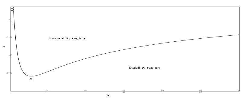
We would like now to describe the stability region for $h$. This is easily done for the special case $a=0$ or $b=0$, see $(i)$ and $(iii)$ of the above proposition. The following result is a description of the VN stability region in the general case.

Corollary 3.1.

There exist real numbers $\tilde{p}>0$ and $\tilde{u}>1$ such that:

• if $-\frac{a}{\left|b\right|_{\infty}^{2}}\geq\tilde{p}$, then (3.3) is true for all $h>0$: the scheme is VN A-stable, recalling Definition 3.1;

• if $-\frac{a}{\left|b\right|_{\infty}^{2}}<\tilde{p}$, there exists $1<\underline{u}<\tilde{u}<\bar{u}<+\infty$ such that the scheme is VN stable if and only if $h\notin\left]\frac{\underline{u}}{\left|b\right|_{\infty}^{2}},\frac{\bar{u}}{\left|b\right|_{\infty}^{2}}\right[$. Moreover, $\underline{u}$ and $\bar{u}$ are respectively an increasing function and a decreasing function of $p=-\frac{a}{\left|b\right|_{\infty}^{2}}$ satisfying

  $${\color[rgb]{0,0,0}\lim_{-\frac{a}{\left|b\right|_{\infty}^{2}}\rightarrow 0}(\underline{u},\bar{u})=(1,+\infty)},\quad\lim_{-\frac{a}{\left|b\right|_{\infty}^{2}}\rightarrow\tilde{p}}(\underline{u},\bar{u})=(\tilde{u},\tilde{u}).$$

Numerically we obtain $\tilde{p}\simeq 0.103417$ and $\tilde{u}=7.35491$.

Proof. Setting $p=-a/\left|b\right|_{\infty}^{2}$ and $u=\left|b\right|_{\infty}^{2}h$, then (3.3) becomes

$$\psi(p,u):=(1+pu)-ue^{\frac{1}{u}-1}\geq 0.$$

The results are then obtained by studying the sign of the function $u\mapsto\psi(p,u)$ for $u\in(0,\infty)$, when $p$ varies in $(0,+\infty)$.     $\sqcap$$\sqcup$

The results of Corollary 3.1 are illustrated in Figure 4, which shows also the point $A=(b.\tilde{p},\tilde{u}/b^{2})$.

Figure 4. Von Neuman stability region, Implicit Euler, $d=1$, $b=5$

Remark 3.1.

1. VN stability regions obtained depend on $\left|b\right|_{\infty}$ and so on the dimension $d$. In particular, the VN A-stability condition is more difficult to fulfill when $d$ is large, and the size of the VN stability region decreases with $d$.

2. The necessary and sufficient VN A-stability condition obtained, namely $-\frac{a}{\left|b\right|_{\infty}^{2}}\geq\tilde{p}$, is much better than the sufficient VN A-stability condition (3.1), namely $-\frac{a}{\left|b\right|^{2}}\geq 0.5{\color[rgb]{0,0,0}d}$.

3.2. Von Neumann stability analysis of the pseudo explicit Euler scheme

We study here the pseudo explicit Euler scheme i.e. the scheme given in Definition 1.1 with $\theta=0$.

Proposition 3.2.

1. If $\left|b\right|=0$, then the scheme is VN stable if and only if $h\leq-\frac{2}{a}$.

2. Assume that $\left|b\right|>0$. Then the scheme is VN stable if and only if $\left|b\right|_{\infty}^{2}h\leq(1+ah)^{2}$ and $h\leq-2/a$, or, $\left|b\right|_{\infty}^{2}h>(1+ah)^{2}$ and

   $$1-\left|b\right|_{\infty}^{2}he^{\frac{(1+ah)^{2}}{\left|b\right|_{\infty}^{2}h}-1}\geq 0.$$ (3.5)

Remark 3.2.

When $a=0$, the same necessary and sufficient condition as in Proposition 3.1(iii) holds true, namely the scheme is VN-stable if and only if $\left|b\right|_{\infty}^{2}h\leq 1$. Indeed, in this case, the implicit scheme and pseudo-explicit scheme are the same.

Proof of Proposition 3.2

Using the same arguments as in the proof of Proposition 3.1, we can write $Y_{i}=y_{i}e^{\mathbf{i}\sum_{\ell=1}^{d}k_{\ell}W^{\ell}_{t_{i}}}$ with $y_{i}\in\mathbb{C}$. Moreover, we compute

$$Y_{i} =\mathbb{E}_{t_{i}}\left[y_{i+1}\left(1+ah+\sum_{\ell=1}^{d}b_{\ell}\Delta W_{i}^{\ell}\right)e^{\mathbf{i}\sum_{\ell=1}^{d}k_{\ell}W^{\ell}_{t_{i+1}}}\right]$$

$$=y_{i+1}\mathbb{E}\left[\left(1+ah+\sum_{\ell=1}^{d}b_{\ell}\Delta W_{i}^{\ell}\right)e^{\mathbf{i}\sum_{\ell=1}^{d}k_{\ell}\Delta W^{\ell}_{i}}\right]e^{\mathbf{i}\sum_{\ell=1}^{d}k_{\ell}W^{\ell}_{t_{i}}}$$

$$=y_{i+1}\left(1+ah+\mathbf{i}h\sum_{\ell=1}^{d}b_{\ell}k_{\ell}\right)e^{-\frac{\sum_{\ell=1}^{d}k_{\ell}^{2}h}{2}}e^{\mathbf{i}\sum_{\ell=1}^{d}k_{\ell}W^{\ell}_{t_{i}}}.$$

Thus we have $Y_{i}=y_{i}e^{\mathbf{i}\sum_{\ell=1}^{d}k_{\ell}W^{\ell}_{t_{i}}}$ with

$$y_{i}=\left(1+ah+\mathbf{i}h\sum_{\ell=1}^{d}b_{\ell}k_{\ell}\right)e^{-\frac{\sum_{\ell=1}^{d}k_{\ell}^{2}h}{2}}y_{i+1}:=\lambda y_{i+1},$$

and so we obtain $Y_{0}=\lambda^{n}$. Recalling Definition 3.1, we get that the scheme is VN stable if and only if, for all $k\in\mathbb{R}^{d}$ we have $\left|\lambda\right|^{2}\leq 1$, i.e.

$$\varphi(x_{1},...,x_{d}):=1-e^{-\sum_{\ell=1}^{d}x_{\ell}}\left((1+ah)^{2}+\left(\sum_{\ell=1}^{d}b_{\ell}\sqrt{x_{\ell}}\right)^{2}h\right)\geq 0,\quad\forall x\in(\mathbb{R}^{+})^{d}.$$ (3.6)

If $|b|=0$, we observe that(3.6) holds true if and only if $\left|1+ah\right|\leq 1$. This proves $(i)$. We now study the case $\left|b\right|>0$. Since $\varphi\leq 1$ and $\lim_{\left|x\right|\rightarrow+\infty}\varphi(x)=1$, we have that $\varphi$ is bounded from above and there exists $\tilde{x}$ such that $\inf_{x\in(\mathbb{R}^{+})^{d}}\varphi(x)=\varphi(\tilde{x})$. Then (3.4) is true if and only if $\varphi(\tilde{x})\geq 0$ and it just remains to find $\tilde{x}$. Using the same reasoning as in the implicit case, we finally show that

1. if $\left|b\right|_{\infty}^{2}h\leq(1+ah)^{2}$ then $\tilde{x}=0$ and so $\varphi(x)\geq\varphi(0)=1-(1+ah)^{2}$ which is positive if and only if $h\leq-2/a$,

2. if $\left|b\right|_{\infty}^{2}h>(1+ah)^{2}$ then

   $$\varphi(x)\geq\varphi(\tilde{x})=1-\left|b\right|_{\infty}^{2}he^{\frac{(1+ah)^{2}}{\left|b\right|_{\infty}^{2}h}-1}.$$

$\sqcap$$\sqcup$

The following Corollary describes the VN stability region more explicitly.

Corollary 3.2.

• If $-\frac{a}{\left|b\right|_{\infty}^{2}}\geq 2$, then the scheme is VN stable if and only if $h\in[0,-2/a]$.

• If $-\frac{a}{\left|b\right|_{\infty}^{2}}<2$, there exists $\overline{h}\in\left[\frac{1}{\left|b\right|_{\infty}^{2}},\frac{-2}{a}\right[$ such that the scheme is VN stable if and only if $h\in[0,\overline{h}]$. $\overline{h}$ is given by the unique solution of the equation

  $$1-\left|b\right|_{\infty}^{2}\overline{h}e^{\frac{(1+a\overline{h})^{2}}{\left|b\right|_{\infty}^{2}\overline{h}}-1}=0.$$

  Moreover, we have

  $$\lim_{-\frac{a}{\left|b\right|_{\infty}^{2}}\rightarrow 0}\overline{h}\left|b\right|_{\infty}^{2}=1,\quad\lim_{-\frac{a}{\left|b\right|_{\infty}^{2}}\rightarrow 2}\overline{h}\frac{\left|a\right|}{2}=1.$$

Proof. Setting $p=-a/\left|b\right|_{\infty}^{2}$ and $u=\left|b\right|_{\infty}^{2}h$, the stability region is obtained studying the sign of the function

$$u\mapsto 1-ue^{\frac{(1-pu)^{2}}{u}-1},\quad u\in\left]\frac{1+2p-\sqrt{1+4p}}{2p^{2}},\frac{1+2p+\sqrt{1+4p}}{2p^{2}}\right[,$$

when $p$ varies in $]0,+\infty[$.     $\sqcap$$\sqcup$

Remark 3.3.

1. Once again VN stability regions obtained depend on $\left|b\right|_{\infty}$ and so on the dimension $d$.

2. Unlike the implicit scheme, the pseudo-explicit scheme is never VN A-stable.

Figure 5. VN stability region, Pseudo-Explicit Euler, $d=1$, $b=5$

4. Numerical illustration

In this section, we illustrate the theoretical results we have obtained previously. In particular, we characterize below the shape of stability and unstability regions for several different examples.

We perform our numerical simulation in the setting of section 1.1 using a trinomial tree (recombining) to approximate the Brownian motion and the terminal condition $\widehat{\xi}=\cos(\widehat{W}_{T})$. Given a constant timestep $h>0$, the increment of the Brownian motion are approximated by discrete random variables $\Delta\widehat{W}_{i}$, $i\leq n$, satisfying

$$\mathbb{P}(\Delta\widehat{W}_{i}=\pm\sqrt{3{h}})=\frac{1}{6}\quad\text{ and }\quad\mathbb{P}(\Delta\widehat{W}_{i}=0)=\frac{2}{3}\;.$$

The $H$-coefficients are given by $H_{i}:=\frac{\Delta\widehat{W}_{i}}{h}$, $i\leq n$, and are bounded. Let us observe that, in the case of the implicit scheme $(\theta=1)$, the stability condition of Proposition 2.2 reads

$$h\leq\frac{1}{3|L^{Z}|^{2}}\;.$$ (4.1)

On the graphs below, we plot the value $|Y_{0}|\wedge 10$ for different values of the parameter $h$ and various specifications of $f$. Contrary to Section 1.1, for a fixed $h$, we chose to run the algorithm using $n=300$, which implicitly sets $T$ to be large. Doing so allows us to observe more clearly the various regions of stability and unstability for the specific choice of $f$, $\hat{\xi}$ and $h$.

4.1. Linear specifications of $f$

On Figures 6 and 7 below, we plot $|Y_{0}|\wedge 10$ for $f(y,z)=ay+5z$, for each $(a,h)\in[-3,0]\times(0,2]$. This quantity corresponds here to the truncated absolute error between the scheme and the true solution, which is approximatively equal to $0$ as $T$ is large.

Figure 6. Empirical stability of pseudo-explicit Euler scheme

Figure 7. Empirical stability of implicit Euler scheme

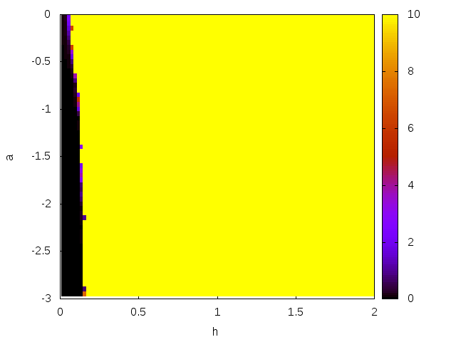
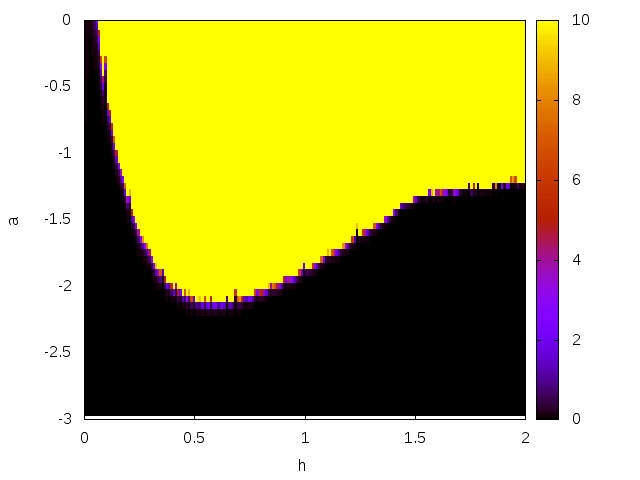
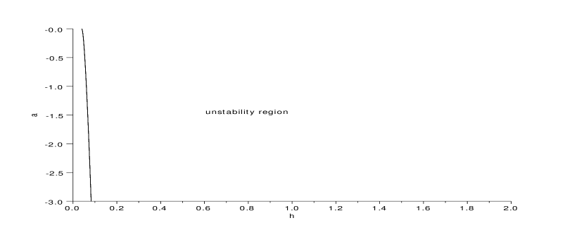
On both graphs, we are able to observe a stability region (in black) and an unstability region (in yellow). The shape of these regions is consistent with the theoretical ones derived in Section 3, compare with Figures 4 and 5.

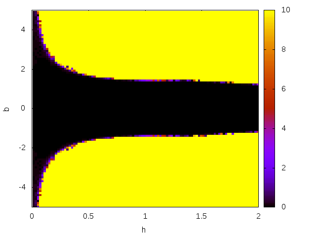
In Figure 8, we consider $f(z)=bz$ for $b\in[-5,5]$ and $h$ which varies between $0$ and $2$.

Figure 8. Empirical stability of Euler scheme $f(y,z)=bz$

4.2. Non linear specifications of $f$

In this section, we investigate the stability of the Euler scheme for some non-linear specification $z\mapsto f(z)$.

4.2.1. $f(z)=b|z|$

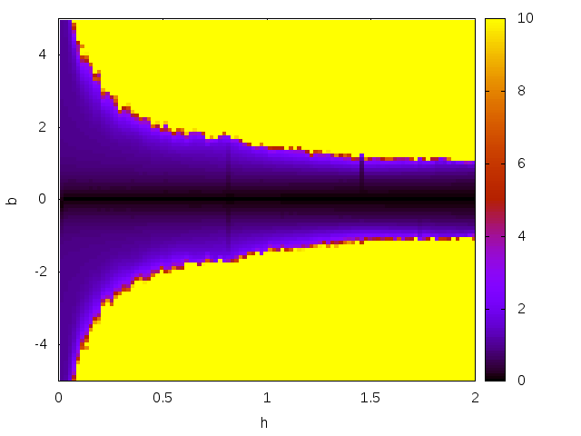
On the graph of Figure 9, we plot the quantity $|Y_{0}|\wedge 10$ for $(b,h)\in[-5,5]\times(0,2]$. In this example, we do not know the true value of $Y$ at time $t=0$. Nevertheless, we can clearly observe the unstability region: in this case, the necessary condition seems to be related to (4.1).

Figure 9. Empirical stability of Euler scheme, $f(z)=b|z|$

4.2.2. $f(z)=atan(bz)$

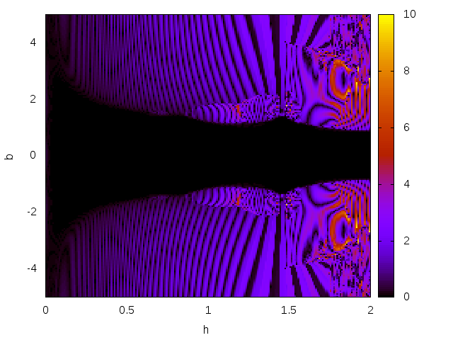
On the plot in Figure 10, we succesfully observe a stability region (in black) of the form predicted by (4.1). Outside this region, the behaviour of the algorithm seems fairly complicated. In particular, the algorithm is not robust outside the black (predicted) stability region as it seems to converge for some values of $h$ and not for others.

Figure 10. Empirical stability of Euler scheme, $f(z)=atan(bz)$

References

- [1] V. Bally and G. Pagès. A quantization algorithm for solving multi-dimensional discrete-time optimal stopping problems. Bernoulli, 9(6):1003–1049, 2003.
- [2] B. Bouchard and N. Touzi. Discrete-time approximation and Monte-Carlo simulation of backward stochastic differential equations. Stochastic Process. Appl., 111(2):175–206, 2004.
- [3] P. Briand, B. Delyon, Y. Hu, É. Pardoux, and L. Stoica. solutions of backward stochastic differential equations. Stochastic Process. Appl., 108(1):109–129, 2003.
- [4] P. Briand, B. Delyon, and J. Mémin. On the robustness of backward stochastic differential equations. Stochastic Process. Appl., 97(2):229–253, 2002.
- [5] P. Briand and Y. Hu. Stability of BSDEs with random terminal time and homogenization of semilinear elliptic PDEs. J. Funct. Anal., 155(2):455–494, 1998.
- [6] D. Brigo, Q. Liu, A. Pallavicini, and D. Sloth. Nonlinear Valuation under Collateral, Credit Risk and Funding Costs: A Numerical Case Study Extending Black-Scholes. ArXiv e-prints, April 2014.
- [7] D. Brigo and A. Pallavicini. CCP Cleared or Bilateral CSA Trades with Initial/Variation Margins under credit, funding and wrong-way risks: A Unified Valuation Approach. ArXiv e-prints, January 2014.
- [8] J. C. Butcher. Numerical methods for ordinary differential equations. John Wiley & Sons Ltd., Chichester, 2003.
- [9] J.-F. Chassagneux. Linear multi-step schemes for BSDEs. arxiv:1306.5548.
- [10] J.-F. Chassagneux and D. Crisan. Runge-kutta schemes for backward stochastic differential equations. The Annals of Applied Probability, 24(2):679–720, 04 2014.
- [11] J.F. Chassagneux and A. Richou. Numerical simulation of quadratic BSDEs. arxiv:1307.5741.
- [12] S. Crépey. Bilateral counterparty risk under funding constraints-part I: Pricing. Mathematical Finance, pages no–no, 2012.
- [13] S. Crépey. Bilateral counterparty risk under funding constraints-part II: CVA. Mathematical Finance, pages no–no, 2012.
- [14] D. Crisan and D. Delarue. Sharp derivative bounds for solutions of degenerate semi-linear partial differential equations. Journal of Functional Analysis, 263(10):3024 – 3101, 2012.
- [15] D. Crisan and K. Manolarakis. Solving backward stochastic differential equations using the cubature method: Application to nonlinear pricing. SIAM Journal on Financial Mathematics, 3(1):534–571, 2012.
- [16] D. Crisan and K. Manolarakis. Second order discretization of backward SDEs and simulation with the cubature method. The Annals of Applied Probability, 24(2):652–678, 04 2014.
- [17] N. El Karoui, S. Peng, and M. C. Quenez. Backward stochastic differential equations in finance. Math. Finance, 7(1):1–71, 1997.
- [18] E. Gobet and C. Labart. Error expansion for the discretization of backward stochastic differential equations. Stochastic Process. Appl., 117(7):803–829, 2007.
- [19] M. Kobylanski. Backward stochastic differential equations and partial differential equations with quadratic growth. Ann. Probab., 28(2):558–602, 2000.
- [20] J.-P. Lepeltier and J. San Martín. Existence for BSDE with superlinear-quadratic coefficient. Stochastics Stochastics Rep., 63(3-4):227–240, 1998.
- [21] A. Lionnet, G. dos Reis, and L. Szpruch. Time discretization of fbsde with polynomial growth drivers and reaction-diffusion pdes. arxiv:1309.2865.
- [22] J. Ma and J. Yong. Forward-Backward Stochastic Differential Equations and Their Applications. Number no. 1702 in Forward-backward Stochastic Differential Equations and Their Applications. Springer, 1999.
- [23] É. Pardoux. BSDEs, weak convergence and homogenization of semilinear PDEs. In Nonlinear analysis, differential equations and control (Montreal, QC, 1998), volume 528 of NATO Sci. Ser. C Math. Phys. Sci., pages 503–549. Kluwer Acad. Publ., Dordrecht, 1999.
- [24] É. Pardoux and S. Peng. Backward stochastic differential equations and quasilinear parabolic partial differential equations. In Stochastic partial differential equations and their applications (Charlotte, NC, 1991), volume 176 of Lecture Notes in Control and Inform. Sci., pages 200–217. Springer, Berlin, 1992.
- [25] É. Pardoux and S. G. Peng. Adapted solution of a backward stochastic differential equation. Systems Control Lett., 14(1):55–61, 1990.
- [26] A. Richou. Markovian quadratic and superquadratic BSDEs with an unbounded terminal condition. Stochastic Process. Appl., 122(9):3173 – 3208, 2012.
- [27] M. Royer. BSDEs with a random terminal time driven by a monotone generator and their links with PDEs. Stoch. Stoch. Rep., 76(4):281–307, 2004.
- [28] J. Zhang. A numerical scheme for BSDEs. Ann. Appl. Probab., 14(1):459–488, 2004.