Statistical Skorohod embedding problem and its generalizations

Abstract

Given a Lévy process $L$, we consider the so-called statistical Skorohod embedding problem of recovering the distribution of an independent random time $T$ based on i.i.d. sample from $L_{T}.$ Our approach is based on the genuine use of the Mellin and Laplace transforms. We propose a consistent estimator for the density of $T,$ derive its convergence rates and prove their optimality. It turns out that the convergence rates heavily depend on the decay of the Mellin transform of $T.$ We also consider the application of our results to the problem of statistical inference for variance-mean mixture models and for time-changed Lévy processes.

Keywords: Skorohod embedding problem, Lévy process, Mellin transform, Laplace transform, variance mixture models, time-changed Lévy processes.

1 Introduction

The so called Skorohod embedding (SE) problem or Skorohod stopping problem was first stated and solved by Skorohod in 1961. This problem can be formulated as follows.

Problem 1.1 (Skorohod Embedding Problem).

For a given probability measure $\mu$ on $\mathbb{R},$ such that $\int|x|d\mu(x)<\infty$ and $\int xd\mu(x)=0,$ find a stopping time $T$ such that $B_{T}\sim\mu$ and $B_{T\wedge t}$ is a uniformly integrable martingale.

The SE problem has recently drawn much attention in the literature, see e.g. Obłój, [11], where the list of references consists of more than 100 items. In fact, there is no unique solution to the SE problem and there are currently more than $20$ different solutions available. This means that from a statistical point of view, the SE problem is not well posed. In this paper we first study what we call statistical Skorohod embedding (SSE) problem.

Problem 1.2 (Statistical Skorohod Embedding Problem).

Based on i.i.d. sample $X_{1},\ldots,X_{n}$ from the distribution of $B_{T}$ consistently estimate the distribution of the random time $T\geq 0,$ where $B$ and $T$ are assumed to be independent.

The independence of $B$ and $T$ is needed to ensure the identifiability of the distribution of $T$ from the distribution of $B_{T}$. It is shown that the SSE problem is closely related to the multiplicative deconvolution problem. Using the Mellin transform technique, we construct a consistent estimator for the density of $T$ and derive its convergence rates in different norms. Furthermore, we show that the obtained rates are optimal in minimax sense. The asymptotic normality of the proposed estimator is addressed as well. Next, we generalize the SSE problem by replacing the standard Brownian motion with a general Lévy process. The generalized SSE problem turns out to be much more involved and its solution requires some new ideas. Using a genuine combination of the Laplace and Mellin transforms, we construct a consistent estimator, derive its minimax convergence rates and prove that these rates basically coincide with the rates in the SSE problem.

Some particular cases of generalized statistical Skorohod embedding problem have been already studied in the literature. For example, the case of the stopped Poisson process was considered in the recent paper of Comte and Genon-Catalot, [6].

2 Statistical Skorohod embedding problem

Let $B$ be a Brownian motion and let a random variable $T\geq 0$ be independent of $B.$ We then have,

(1) $$X:=B_{T}\sim\sqrt{T}\,B_{1}$$

and the problem of reconstructing $T$ is related to a multiplicative deconvolution problem. While for additive deconvolution problems the Fourier transform plays an important role, here we can conveniently use the Mellin transform.

Definition 2.1.

Let $\xi$ be a non-negative random variable with a probability density $p_{\xi}$, then the Mellin transform of $p_{\xi}$ is defined via

(2) $$\mathcal{M}[p_{\xi}](z):=\mathbb{E}[\xi^{z-1}]=\int_{0}^{\infty}p_{\xi}(x)x^{z-1}\,dx$$

for all $z\in\mathcal{S}_{\xi}$ with $\mathcal{S}_{\xi}=\bigl{\{}z\in\mathbb{C}:\mathbb{E}[\xi^{\mathsf{Re}z-1}]<\infty\bigr{\}}.$

Since $p_{\xi}$ is a density, it is integrable and so at least $\left\{z\in\mathbb{C}:\mathsf{Re}(z)=1\right\}\subset\mathcal{S}_{\xi}.$ Under mild assumptions on the growth of $p_{\xi}$ near the origin, one obtains

$$\left\{z\in\mathbb{C}:0\leq a_{\xi}<\mathsf{Re}(z)<b_{\xi}\right\}\subset\mathcal{S}_{\xi}$$

for some $0\leq a_{\xi}<1\leq b_{\xi}.$ Then the Mellin transform (2) exists and is analytic in the strip $a_{\xi}<\operatorname{Re}z<b_{\xi}.$ For example, if $p_{\xi}$ is essentially bounded in a right-hand neighborhood of zero, we may take $a_{\xi}=0.$ The role of the Mellin transform in probability theory is mainly related to the product of independent random variables: in fact it is well-known that the probability density of the product of two independent random variables is given by the Mellin convolution of the two corresponding densities. Due to (1), the SSE problem is closely connected to the Mellin convolution. Suppose that the random time $T$ has a density $p_{T}$ and that we may take $0\leq a_{T}<1\leq b_{T}.$ Since $\mathcal{S}_{|B_{1}|}\supset\left\{z\in\mathbb{C}:\mathsf{Re}(z)>0\right\},$ we derive for $\max(2a_{T}-1,0)<\mathsf{Re}(z)<2b_{T}-1,$

$$\mathcal{M}[p_{|X|}](z)=\mathbb{E}\bigl{[}|B_{1}|^{z-1}\bigr{]}\mathbb{E}\bigl{[}T^{(z-1)/2}\bigr{]}\\ =\mathcal{M}[p_{|B_{1}|}](z)\mathcal{M}[p_{T}]((z+1)/2)=\frac{2^{(z-1)/2}}{\sqrt{\pi}}\Gamma(z/2)\mathcal{M}[p_{T}]((z+1)/2).$$

As a result

$$\mathcal{M}[p_{T}](z)=\frac{\sqrt{\pi}}{2^{z-1}}\frac{\mathcal{M}[p_{|X|}](2z-1)}{\Gamma(z-1/2)},\text{ \ \ }\max(a_{T},1/2)<\mathsf{Re}(z)<b_{T}$$

and the Mellin inversion formula yields

(3) $$p_{T}(x) =\frac{1}{2\pi}\int_{\gamma-{\mathrm{i}}\infty}^{\gamma+{\mathrm{i}}\infty}x^{-\gamma-{\mathrm{i}}v}\mathcal{M}[p_{T}](\gamma+{\mathrm{i}}v)\,dv\text{ }$$

$$=\frac{1}{\sqrt{\pi}}\int_{-\infty}^{\infty}x^{-\gamma-{\mathrm{i}}v}\frac{\mathcal{M}[p_{|X|}](2\left(\gamma+{\mathrm{i}}v\right)-1)}{2^{\gamma+{\mathrm{i}}v}\Gamma(\gamma+{\mathrm{i}}v-1/2)}\,dv\text{\ \ for \ }\max(a_{T},1/2)<\gamma<b_{T},\text{ \ \ }x>0.$$

Furthermore, the Mellin transform of $p_{|X|}$ can be directly estimated from the data $X_{1},\ldots,X_{n}$ via the empirical Mellin transform:

(4) $$\mathcal{M}_{n}[p_{|X|}](z):=\frac{1}{n}\sum_{k=1}^{n}|X_{k}|^{z-1},\text{ \ \ }\mathsf{Re}(z)>1/2,$$

where the condition $\mathsf{Re}(z)>1/2$ guarantees that the variance of the estimator (4) is finite. Note however that the integral in (3) may fail to exist if we replace $\mathcal{M}[p_{|X|}]$ by $\mathcal{M}_{n}[p_{|X|}].$ We so need to regularize the inverse Mellin operator. To this end, let us consider a kernel $K(\cdot)\geq 0$ supported on $[-1,1]$ and a sequence of bandwidths $h_{n}$ $>0$ tending to $0$ as $n\rightarrow\infty.$ Then we define, in view of (4), for some $\max(a_{T},3/4)<\gamma<b_{T},$

(5) $$p_{T,n}(x):=\frac{1}{\sqrt{\pi}}\int_{-\infty}^{\infty}x^{-\gamma-{\mathrm{i}}v}K(vh_{n})\frac{\mathcal{M}_{n}[p_{|X|}](2(\gamma+{\mathrm{i}}v)-1)}{2^{\gamma+{\mathrm{i}}v}\Gamma(\gamma-1/2+{\mathrm{i}}v)}\,dv.$$

For our convergence analysis, we will henceforth take the simplest kernel

$$K(y)=1_{[-1,1]}(y),$$

but note that in principle other kernels may be considered as well. The next theorem states that $p_{T,n}$ converges to $p_{T}$ at a polynomial rate, provided the Mellin transform of $p_{T}$ decays exponentially fast. We shall use throughout the notation $A\lesssim B$ if $A$ is bounded by a constant multiple of $B$, independently of the parameters involved, that is, in the Landau notation $A=O(B)$.

Theorem 2.2.

For any $\beta>0,$ $\gamma>0$ and $L>0$, introduce the class of functions

$$\mathcal{C}(\beta,\gamma,L)=\left\{f:\int_{-\infty}^{\infty}\left|\mathcal{M}[f](\gamma+{\mathrm{i}}v)\right|e^{\beta\left|v\right|}\,dv<L\right\}.$$

Assume that $p_{T}\in\mathcal{C}(\beta,\gamma,L)$ for some $\beta>0,$ $L>0$ and

(6) $$\max((a_{T}+1)/2,3/4)<\gamma<b_{T}.$$

Then for some constant $C_{\gamma,L}$ depending on $\gamma$ and $L$ only, it holds

(7) $$\sup_{x\geq 0}\mathbb{E}\Bigl{[}\bigl{\{}x^{\gamma}|p_{T}(x)-p_{T,n}(x)|\bigr{\}}^{2}\Bigr{]}\leq C_{\gamma,L}\times\begin{cases}e^{-2\beta/h_{n}}+\frac{1}{n}h_{n}^{2\left(\gamma-1\right)}e^{\pi/h_{n}},&\gamma<1,\\ e^{-2\beta/h_{n}}+\frac{1}{n}e^{\pi/h_{n}},&\gamma\geq 1.\end{cases}$$

By next choosing

(8) $$h_{n}=\begin{cases}\frac{\pi+2\beta}{\log n-2(1-\gamma)\log\log n},&\gamma<1,\\ (\pi+2\beta)/\log n,&\gamma\geq 1,\end{cases}$$

we arrive at the rate

(9) $$\sup_{x\geq 0}\sqrt{\mathbb{E}\Bigl{[}\bigl{\{}x^{\gamma}|p_{T}(x)-p_{T,n}(x)|\bigr{\}}^{2}\Bigr{]}}\lesssim\begin{cases}n^{-\frac{\beta}{\pi+2\beta}}\log^{\frac{2(1-\gamma)\beta}{\pi+2\beta}}n,&\gamma<1,\\ n^{-\frac{\beta}{\pi+2\beta}},&\gamma\geq 1\end{cases}$$

as $n\rightarrow\infty.$

With a little bit more effort one can prove the strong uniform convergence of the estimate $p_{n,T}.$

Theorem 2.3.

Under conditions of Theorem 2.2 and for $\gamma<1$

$$\sup_{p_{T}\in\mathcal{C}(\beta,\gamma,L)}\sup_{x\geq 0}\bigl{\{}x^{\gamma}|p_{T,n}(x)-p_{T}(x)|\bigr{\}}=O_{a.s.}\left(n^{-\frac{\beta}{\pi+2\beta}}\log^{\frac{2(1-\gamma)\beta}{\pi+2\beta}}n\right).$$

Let us turn now to some examples.

Example 2.4.

Consider the class of Gamma densities

$$p_{T}(x;\alpha)=\frac{x^{\alpha-1}\cdot e^{-x}}{\Gamma(\alpha)},\quad x\geq 0$$

for $\alpha>0.$ Since

$$\mathcal{M}[p_{T}](z)=\frac{\Gamma(z+\alpha-1)}{\Gamma(\alpha)},\quad\mathsf{Re}(z)>0,$$

we derive that $p_{T}\in\mathcal{C}(\beta,\gamma,L)$ for all $0<\beta<\pi/2,$ $\gamma>0$ and some $L=L(\beta,\gamma)$ due to the asymptotic properties of the Gamma function (see Lemma 7.3 in Appendix). As a result, Theorem 2.2 implies

$$\sup_{x\geq 0}\sqrt{\mathbb{E}\Bigl{[}\bigl{\{}x^{\gamma}|p_{T}(x)-p_{T,n}(x)|\bigr{\}}^{2}\Bigr{]}}\lesssim n^{-\rho},\quad n\rightarrow\infty$$

for any $\rho<1/4,$ provided $\gamma\geq 1.$

Example 2.5.

Let us look at the family of densities

$$p_{T}(x;q)=\frac{q\sin(\pi/q)}{\pi}\frac{1}{1+x^{q}},\quad q\geq 2,\quad x\geq 0.$$

We have

$$\mathcal{M}[p_{T}](z)=\frac{\sin(\pi/q)}{\sin(\pi z/q)},\quad 0<\mathsf{Re}(z)<q.$$

Therefore, $p_{T}\in\mathcal{C}(\beta,\gamma,L)$ for all $0<\beta<\pi/q,$ $\gamma>0$ and $L=L(\beta,\gamma),$ implying

$$\sup_{x\geq 0}\sqrt{\mathbb{E}\Bigl{[}\bigl{\{}x^{\gamma}|p_{T}(x)-p_{T,n}(x)|\bigr{\}}^{2}\Bigr{]}}\lesssim n^{-\rho},\quad n\rightarrow\infty$$

for any $\rho<1/(2+q),$ provided $\gamma\geq 1.$

If $\mathcal{M}[p_{T}]$ decays polynomially fast, we get the following result.

Theorem 2.6.

Consider the class of functions

$$\mathcal{D}(\beta,\gamma,L)=\left\{f:\int_{-\infty}^{\infty}\left|\mathcal{M}[f](\gamma+{\mathrm{i}}v)\right|(1+|v|^{\beta})\,dv<L\right\},$$

and assume that $p_{T}\in\mathcal{D}(\beta,\gamma,L)$ for some $\beta>0$ and $L>0$ and $\gamma$ as in (6). Then for some constant $D_{\gamma,L},$ it holds

(10) $$\sup_{x\geq 0}\mathbb{E}\Bigl{[}\bigl{\{}x^{\gamma}|p_{T}(x)-p_{T,n}(x)|\bigr{\}}^{2}\Bigr{]}\leq D_{\gamma,L}\times\begin{cases}h_{n}^{2\beta}+\frac{1}{n}h_{n}^{2\left(\gamma-1\right)}e^{\pi/h_{n}},&\gamma<1,\\ h_{n}^{2\beta}+\frac{1}{n}e^{\pi/h_{n}},&\gamma\geq 1.\end{cases}$$

By choosing

(11) $$h_{n}=\frac{\pi}{\log n-2\left(\beta+1-\gamma\right)\log\log n},$$

if $\gamma<1$ and

(12) $$h_{n}=\frac{\pi}{\log n-2\beta\log\log n}$$

for $\gamma\geq 1,$ we arrive at

(13) $$\sup_{x\geq 0}\sqrt{\mathbb{E}\Bigl{[}\bigl{\{}x^{\gamma}|p_{T}(x)-p_{T,n}(x)|\bigr{\}}^{2}\Bigr{]}}\lesssim\log^{-\beta}(n),\quad n\rightarrow\infty.$$

Remark 2.7.

Due to the relation

$$\mathcal{M}[p_{T}](\gamma+{\mathrm{i}}v)=\mathcal{F}[e^{\gamma\cdot}p_{T}(e^{\cdot})](v),\quad a_{T}<\gamma<b_{T},$$

the conditions $p_{T}\in\mathcal{C}(\beta,\gamma,L)$ and $p_{T}\in\mathcal{D}(\beta,\gamma,L)$ are closely related to the smoothness properties of the function $e^{\gamma x}p_{T}(e^{x}).$ For example, if $p_{T}\in\mathcal{C}(\beta,\gamma,L),$ then

$$\int_{-\infty}^{\infty}\left|\mathcal{F}[e^{\gamma\cdot}p_{T}(e^{\cdot})](v)\right|e^{\beta\left|v\right|}\,dv<L$$

and the function $e^{\gamma x}p_{T}(e^{x})$ is called supersmooth in this case, see Meister [9] for the discussion on different smoothness classes in the context of the additive deconvolution problems.

$\mathcal{C}(\beta,\gamma,L)$		$\mathcal{D}(\beta,\gamma,L)$
$\gamma<1$	$\gamma\geq 1$
$n^{-\frac{\beta}{\pi+2\beta}}\log^{\frac{2(1-\gamma)\beta}{\pi+2\beta}}(n)$	$n^{-\frac{\beta}{\pi+2\beta}}$	$\log^{-\beta}(n)$

Table 1: Minimax rates of convergence for the classes $\mathcal{C}(\beta,\gamma,L)$ and $\mathcal{D}(\beta,\gamma,L).$

The rates of Theorem 2.2 and Theorem 2.6 summarized in Table 1 are in fact optimal (up to a logarithmic factor) in minimax sense for the classes $\mathcal{C}(\beta,\gamma,L)$ and $\mathcal{D}(\beta,\gamma,L),$ respectively.

Theorem 2.8.

Fix some $\beta>1.$ There are $\varepsilon>0$ and $x>0$ such that

$$\liminf_{n\to\infty}\inf_{p_{n}}\sup_{p_{T}\in\mathcal{C}(\beta,\gamma,L)}\operatorname{P}^{\otimes n}_{p_{T}}\Bigl{(}|p_{T}(x)-p_{n}(x)|\geq\varepsilon\,n^{-\frac{\beta}{\pi+2\beta}}\log^{-\rho}(n)\Bigr{)}>0,$$

$$\liminf_{n\to\infty}\inf_{p_{n}}\sup_{p_{T}\in\mathcal{D}(\beta,\gamma,L)}\operatorname{P}^{\otimes n}_{p_{T}}\Bigl{(}|p_{T}(x)-p_{n}(x)|\geq\varepsilon\log^{-\beta}(n)\Bigr{)}>0,$$

for some $\rho>0,$ where the infimum is taken over all estimators (i.e. all measurable functions of $X_{1},\ldots,X_{n}$) of $p_{T}$ and $\operatorname{P}^{\otimes n}_{p_{T}}$ is the distribution of the i.i.d. sample $X_{1},\ldots,X_{n}$ with $X_{1}\sim W_{T}$ and $T\sim p_{T}.$

2.1 Asymptotic normality

In the case of $K(v)=1_{[-1,1]}(v),$ the estimate $p_{T,n}(x)$ can be written as

$$p_{T,n}(x) :=\frac{1}{\sqrt{\pi}}\int_{-1/h_{n}}^{1/h_{n}}\left[\frac{1}{n}\sum_{k=1}^{n}|X_{k}|^{2(\gamma+\mathrm{i}v-1)}\right]\frac{x^{-\gamma-\mathrm{i}v}}{2^{\gamma+\mathrm{i}v}\Gamma(\gamma-1/2+\mathrm{i}v)}\,dv$$

$$=\frac{1}{n}\sum_{k=1}^{n}Z_{n,k}$$

where

$$Z_{n,k}:=\frac{1}{\sqrt{\pi}}\int_{-1/h_{n}}^{1/h_{n}}|X_{k}|^{2(\gamma+\mathrm{i}v-1)}\frac{x^{-\gamma-\mathrm{i}v}}{2^{\gamma+\mathrm{i}v}\Gamma(\gamma-1/2+\mathrm{i}v)}\,dv.$$

The following theorem holds

Theorem 2.9.

Suppose that

$$\left.\frac{d}{du}\left(\Gamma(2\gamma-3/2+\mathrm{i}u)\mathcal{M}[p_{T}](2\gamma-1+\mathrm{i}u)\right)\right|_{u=0}\neq 0,$$

and

$$\int_{-\infty}^{\infty}\left|\mathcal{M}[p_{T}](2\gamma-1+\mathrm{i}u)\right|du<\infty,$$

then

$$\rho^{-1}_{n}\bigl{(}p_{T,n}(x)-\mathbb{E}[p_{T,n}(x)]\bigr{)}\overset{\mathcal{D}}{\longrightarrow}\mathcal{N}(0,\sigma^{2})$$

for some $\sigma^{2}>0,$ where $\rho_{n}=n^{-1/2}h_{n}^{2\left(\gamma-1\right)}\log^{-2}\left(1/h_{n}\right)\exp\left[\pi/h_{n}\right](1+o(1))$ and $h_{n}\asymp c\log^{-1}(n)$ for some $c>0,$ as $n\to\infty.$

3 Generalised statistical Skorohod embedding problem

In this section we generalize the statistical Skorohod embedding problem to the case of Lévy processes. In particular, we consider the following problem.

Problem 3.1.

Based on i.i.d. sample $X_{1},\ldots,X_{n}$ from the distribution of $\mu,$ estimate the distribution of the random time $T\geq 0$ independent of a Lévy process $L$ such that $L_{T}\sim\mu.$

Note that the situation here is much more difficult than before, since the Lévy processes do not have, in general, the scaling property (1). Hence the approach based on the Mellin deconvolution technique can not be applied any longer. Let $(L_{t},\,t\geq 0)$ be a Lévy process with the triplet $(\mu,\sigma^{2},\nu).$ Define a curve in $\mathbb{C}$

$$\ell:=\Bigl{\{}\mathsf{Re}(\psi(u))+{\mathrm{i}}\,\mathsf{Im}(\psi(u)),\,u\in\mathbb{R}_{+}\Bigr{\}},$$

where $\psi(u)=-t^{-1}\log(\mathbb{E}(\exp(\mathrm{i}uL_{t}))).$ Our approach to reconstruct the distribution of $T$ is based on the simple identity

(14) $$\mathcal{F}[p_{X}](\lambda)=\mathbb{E}[\exp({\mathrm{i}}\lambda L_{T})]=\mathcal{L}[p_{T}](\psi(\lambda)).$$

It is well known that the Laplace transform of $\mathcal{L}[p_{T}](u)$ is analytic in the domain $\bigl{\{}\mathsf{Re}(u)>0\bigr{\}}.$

Figure 1: A typical shape of the contour $\ell$.

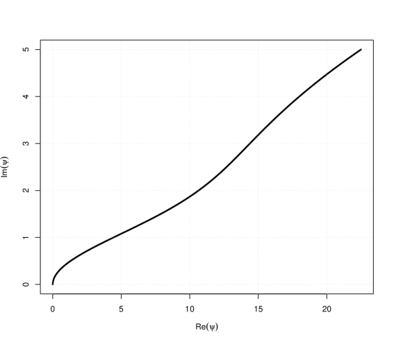
The following proposition shows that the object $\mathcal{M}[\mathcal{L}[p_{T}]](z)$ is well defined and that it can be related to the Fourier transform of $p_{X},$ which in turn can be estimated from the data.

Proposition 3.2.

Let us assume that $\mathsf{Re}(\psi(u))\rightarrow\infty$ as $u\rightarrow\infty$ and that

(15) $$\frac{\left|\mathsf{Im}(\psi(u))\right|}{\mathsf{Re}(\psi(u))}<A<\infty$$

for all $u>0$ and some $A>0.$ Moreover, let $p_{T}$ be (essentially) bounded. Then, for $0<\mathsf{Re}(z)<1$ it holds that

$$\mathcal{M}[\mathcal{L}[p_{T}]](z)=\int_{0}^{\infty}u^{z-1}\mathcal{L}[p_{T}](u)du=\int_{\ell}w^{z-1}\mathcal{L}[p_{T}](w)dw.$$

Remark 3.3.

The condition (15) is fulfilled if, for example, the diffusion part of $L$ is nonzero or if $\psi$ is real and $\psi(u)\to\infty$ as $u\to\infty.$

Under the assumptions of Proposition 3.2 we may write,

$$\mathcal{M}[\mathcal{L}[p_{T}]](z)=\int_{0}^{\infty}\left[\psi(\lambda)\right]^{z-1}\mathcal{L}[p_{T}](\psi(\lambda))\psi^{\prime}(\lambda)d\lambda,$$

where $\mathcal{L}[p_{T}](\psi(\lambda))=\mathcal{F}[p_{X}](\lambda)$ due to (14). On other hand, one may straightforwardly derive,

$$\mathcal{M}[\mathcal{L}[p_{T}]](z)=\mathcal{M}[p_{T}](1-z)\Gamma(z),\quad 0<\mathsf{Re}(z)<1,$$

i.e.,

(16) $$\mathcal{M}[p_{T}](z)=\frac{\mathcal{M}[\mathcal{L}[p_{T}]](1-z)}{\Gamma(1-z)}=\frac{\int_{0}^{\infty}\left[\psi(\lambda)\right]^{-z}\mathcal{F}[p_{X}](\lambda)\psi^{\prime}(\lambda)d\lambda}{\Gamma(1-z)},\quad 0<\mathsf{Re}(z)<1.$$

In principle, one can now replace the Fourier transform of $p_{X}$ in (16) by its empirical counterpart based on the data. However, in this case we need to regularize the estimate of $\mathcal{M}[p_{T}](z)$ to perform the inverse Mellin transform. To this end consider the approximation

$$\mathcal{M}[\mathcal{L}[p_{T}]](z)\approx\frac{1}{n}\sum_{k=1}^{n}\int_{0}^{A_{n}}\left[\psi(\lambda)\right]^{z-1}e^{{\mathrm{i}}X_{k}\lambda}\psi^{\prime}(\lambda)d\lambda=:\frac{1}{n}\sum_{k=1}^{n}\Phi_{n}(z,X_{k})$$

and define in view of (16),

(17) $$p_{T,n}(x):=\frac{1}{2\pi n}\sum_{k=1}^{n}\int_{-U_{n}}^{U_{n}}\frac{\Phi_{n}(1-\gamma-{\mathrm{i}}v,X_{k})}{\Gamma(1-\gamma-{\mathrm{i}}v)}x^{-\gamma-\mathrm{i}v}dv,\text{ \ \ for \ }0<\gamma<1\text{\ }$$

where $U_{n},A_{n}\rightarrow\infty$ in a suitable way as $n\rightarrow\infty.$ Note that in many cases the function $\Phi_{n}$ can be found in closed form. For example, consider the case of a subordinated stable Lévy process with $\psi(\lambda)=|\lambda|^{\alpha}.$ It then holds for $\mathsf{Re}(z)>0,$

$$\Phi_{n}(z,x) =\int_{0}^{A_{n}}\left[\psi(\lambda)\right]^{z-1}e^{{\mathrm{i}}x\lambda}\psi^{\prime}(\lambda)d\lambda$$

$$=\alpha\int_{0}^{A_{n}}\lambda^{\alpha(z-1)}e^{{\mathrm{i}}x\lambda}\lambda^{\alpha-1}\,d\lambda$$

$$=\alpha\int_{0}^{A_{n}}\lambda^{\alpha z-1}e^{{\mathrm{i}}x\lambda}d\lambda$$

$$=\frac{A_{n}^{\alpha z}}{z}F_{1}(\alpha z;1+\alpha z;{\mathrm{i}}A_{n}x),$$

where $F_{1}$ is Kummer’s function. In the next two theorems we prove a remarkable result showing that the estimate $p_{T,n}(x)$ converges to $p(x)$ at the same rate (up to a logarithmic factor in the polynomial case) as in the case of the time-changed Brownian motion.

Theorem 3.4.

Suppose that $\psi$ satisfies the conditions of Proposition 3.2, and that moreover $\int_{\{|x|>1\}}|x|\nu(dx)<\infty.$ Furthermore suppose that there is a $1/2<\gamma<1$ such that $p_{T}\in\mathcal{C}(\beta,\gamma,L)$ (cf. Theorem 2.2) for some $\beta>0,$ and

(18) $$\int_{{1}}^{\infty}\frac{1}{\lambda^{2\gamma-1-\varepsilon}}\left|\mathcal{F}[p_{X}](\lambda)\right|d\lambda<\infty,$$

for some $\varepsilon>0.$ Then under the choice

(19) $$A_{n}=n^{\frac{1}{4\left(1-\gamma\right)+2\varepsilon}}$$

and

(20) $$U_{n}=\frac{\varepsilon}{\left(2-2\gamma+\varepsilon\right)\left(2\beta+\pi\right)}\log n-\frac{2\gamma-1}{2\beta+\pi}\log\log n,$$

we get

(21) $$\sup_{x\geq 0}\sqrt{\mathrm{E}\left[x^{2\gamma}\left|p_{T,n}(x)-p_{T}(x)\right|^{2}\right]}\lesssim n^{-\frac{\beta}{2\beta+\pi}\frac{\varepsilon}{2\left(1-\gamma\right)+\varepsilon}}\log^{\beta\frac{2\gamma-1}{2\beta+\pi}}n,\quad n\rightarrow\infty.$$

Thus for $\gamma\to 1$ or $\varepsilon\to 0,$ we recover the rates of Theorem 2.2 up to a logarithmic factor.

Remark 3.5.

Since

$$\int_{1}^{\infty}\frac{1}{\lambda^{2\gamma-1-\varepsilon}}\left|\mathcal{F}[p_{X}](\lambda)\right|d\lambda=\int_{1}^{\infty}\frac{1}{\lambda^{2\gamma-1-\varepsilon}}\left|\mathcal{L}[p_{T}](\psi(\lambda))\right|d\lambda,$$

the condition (18) is, for example, fulfilled for some $\varepsilon>0$ if $\mathsf{Re}[\psi(\lambda)]\gtrsim\lambda$ for $\lambda\to+\infty$ and $p_{T}$ is of bounded variation with $p_{T}(0)<\infty.$

In the case $p_{T}\in\mathcal{D}(\beta,\gamma,L),$ we get exactly the same logarithmic rates as in Theorem 2.6.

Theorem 3.6.

Suppose that $\psi$ and $\gamma$ are as in Theorem 3.4, and that now $p_{T}\in\mathcal{D}(\beta,\gamma,L)$ (cf. Theorem 2.6) for some $\beta>0.$ Further suppose that (18) holds. Then under the choice

(22) $$A_{n}=n^{\frac{1}{4\left(1-\gamma\right)+2\varepsilon}}$$

(hence the same as in Theorem 3.4) and

(23) $$U_{n}=\frac{\varepsilon}{\pi\left(2-2\gamma+\varepsilon\right)}\log n-\frac{2\beta+2\gamma-1}{\pi}\log\log n,$$

we get

$$\sup_{x\geq 0}\sqrt{\mathrm{E}\left[x^{2\gamma}\left|p_{T,n}(x)-p_{T}(x)\right|^{2}\right]}\lesssim\log^{-\beta}(n),\quad n\rightarrow\infty.$$

Discussion

The rates in Theorem 3.4 and Theorem 3.6 are optimal in minimax sense, since they are basically coincides (up to a logarithmic factor) with the rates in Theorem 2.2 and Theorem 2.6, respectively. As can be seen from the proof of Theorem 2.8 and Remark 3.5, the lower bonds continue to hold true under the additional assumption (18). Let us also stress that the class $\mathcal{C}(\beta,\gamma,L)$ is quite large and contains the well known families of distributions such as Gamma, Beta and Weibull families. It follows from Theorem 3.4 that for all these families our estimator $p_{n,T}$ converges at a polynomial rate.

4 Applications

4.1 Estimation of the variance-mean mixture models

The variance-mean mixture of the normal distribution is defined as

$$p(x)=\int_{0}^{\infty}(2\pi\sigma^{2}u)^{-1/2}\exp(-(x-\mu u)^{2}/(2\sigma^{2}u))\,g(u)du,$$

where $g(u)$ is a mixing density on $\mathbb{R}_{+}.$ The variance-mean mixture models play an important role in both the theory and the practice of statistics. In particular, such mixtures appear as limit distributions in asymptotic theory for dependent random variables and they are useful for modeling data stemming from heavy-tailed and skewed distributions, see, e.g. [1] and [3]. As can be easily seen, the variance-mean mixture distribution $p$ coincides with the distribution of the random variable $\sigma W_{T}+\mu T,$ where $T$ is the random variable with density $g,$ which is independent of $W.$ The class of variance-mean mixture models is rather large. For example, the class of the normal variance mixture distributions ($\mu=0$) can be described as follows: $p$ is the density of a normal variance mixture (equivalently $p$ is the density of $W_{T}$) if and only if $\mathcal{F}[p](\sqrt{u})$ is a completely monotone function in $u.$ The problem of statistical inference for variance-mean mixture models has been already considered in the literature. For example, Korsholm, [8] proved the consistency of the non-parametric maximum likelihood estimator for the parameters $\sigma$ and $\mu,$ $g$ being treated as an infinite dimensional nuisance parameter. In Zhang [14] the problem of estimating the mixing density in location (mean) mixtures was studied. To the best of our knowledge, we here address, for the first time, the problem of non-parametric inference for the mixing density $g$ in full generality and derive the minimax convergence rates. In fact, Theorem 3.4 and Theorem 3.6 directly apply not only to normal variance-mean mixture models, but also to stable variance-mean mixtures.

4.2 Estimation of time-changed Lévy models

Let $L=(L_{t})_{t\geq 0}$ be a one-dimensional Lévy process and let $\mathcal{T}=(\mathcal{T}(s))_{s\geq 0}$ be a non-negative, non-decreasing stochastic process independent of $X$ with $\mathcal{T}(0)=0$. A time-changed Lévy process $Y=(Y_{s})_{s\geq 0}$ is then defined as $Y_{s}=X_{\mathcal{T}(s)}.$ The process $\mathcal{T}$ is usually referred to as time change or subordinator. Consider the problem of statistical inference on the distribution of the time change $\mathcal{T}$ based on the low-frequency observations of the time-changed Lévy process $X_{t}=L_{\mathcal{T}(t)}.$ Suppose that $n$ observations of the Lévy process $L_{t}$ at times $t_{j}=j\Delta,$ $j=0,\ldots,n,$ are available. If the sequence $\mathcal{T}(t_{j})-\mathcal{T}(t_{j-1}),$ $j=1,\ldots,n,$ is strictly stationary with the invariant stationary distribution $\pi,$ then for any bounded “test function” $f,$

(24) $$\frac{1}{n}\sum_{j=1}^{n}f\left(L_{\mathcal{T}(t_{j})}-L_{\mathcal{T}(t_{j-1})}\right)\to\mathbb{E}_{\pi}[f(L_{\mathcal{T}(\Delta)})],\quad n\to\infty,$$

The limiting expectation in (24) is then given by

$$\mathbb{E}_{\pi}[f(L_{\mathcal{T}(\Delta)})]=\int_{0}^{\infty}\mathbb{E}[f(L_{s})]\,\pi(ds).$$

Taking $f(z)=f_{u}(z)=\exp(\mathrm{i}u^{\top}z),$ $u\in\mathbb{R}^{d},$ we arrive at the the following representation for the c.f. of $L_{\mathcal{T}(s)}$:

(25) $$\mathbb{E}\left[\exp\left(\mathrm{i}uL_{\mathcal{T}(\Delta)}\right)\right]=\int_{0}^{\infty}\exp(t\psi(u))\,\pi(dt)=\mathcal{L}_{\pi}(\psi(u)),$$

where $\psi(u):=-t^{-1}\log(\phi_{t}(u))$ with $\phi_{t}(u)=\mathbb{E}\exp(\mathrm{i}u^{\top}L_{t})$ being the characteristic exponent of the Lévy process $L$ and $\mathcal{L}_{\pi}$ being the Laplace transform of $\pi.$ Suppose we want to estimate the invariant measure $\pi$ (or its density) from the discrete time observations of $L_{\mathcal{T}},$ then we are in the setting of the generalized statistical Skorohod embedding with the only difference that the elements of the sample $L_{\mathcal{T}(t_{1})}-L_{\mathcal{T}(t_{0})},\ldots,L_{\mathcal{T}(t_{n})}-L_{\mathcal{T}(t_{n-1})}$ are not necessarily independent. However, under appropriate mixing properties of the sequence $\mathcal{T}(t_{j})-\mathcal{T}(t_{j-1}),$ $j=1,\ldots,n,$ one can easily generalize the results of Section 3 to the case of dependent data (see, e.g. [2] for similar results). The problem of estimating the parameters of a Lévy process observed at low frequency was considered in Neumann and Reiß, [10] and Chen et al, [5]. Let us note that the statistical inference for time-changed Lévy processes based on high-frequency observations of $Y$ has been the subject of many studies, see, e.g. Bull, [4] and Todorov and Tauchen, [12] and the references therein.

5 Numerical examples

Barndorff-Nielsen et al. [1] consider a class of variance-mean mixtures of normal distributions which they call generalized hyperbolic distributions. The univariate and symmetric members of this family appear as normal scale mixtures whose mixing distribution is the generalized inverse Gaussian distribution with density

(26) $$p_{T}(v)=\frac{(\varkappa/\delta)^{\lambda}}{2K_{\lambda}(\delta\varkappa)}v^{\lambda-1}\exp\left(-\frac{1}{2}\left(\varkappa^{2}v+\frac{\delta^{2}}{v}\right)\right),\quad v>0,$$

for some $\varkappa,$ $\delta\geq 0$ and $\lambda>0,$ where $K$ is a modified Bessel function. The resulting normal scale mixture has probability density function

$$p_{X}(x)=\frac{\varkappa^{1/2}}{(2\pi)^{1/2}\delta^{\lambda}}K_{\lambda}(\delta\varkappa)(\delta^{2}+x^{2})^{\frac{1}{2}\left(\lambda-\frac{1}{2}\right)}K_{\lambda-\frac{1}{2}}\bigl{(}\varkappa(\delta^{2}+x^{2})^{1/2}\bigr{)}.$$

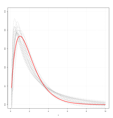
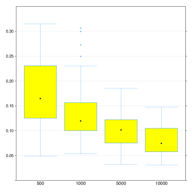
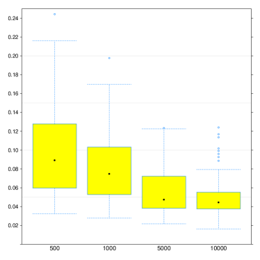
Let us start with a simple example, Gamma density $p_{T}(x)=x\exp(-x),$ $x\geq 0,$ which is a special case of (26) for $\delta=0,$ $\lambda=2$ and $\varkappa=\sqrt{2}.$ We simulate a sample of size $n$ from the distribution of $X,$ and construct the estimate (5) with the bandwidth $h_{n}$ given (up to a constant not depending on $n$) by (8) and $\gamma=0.8.$ In Figure 2 (left), one can see $50$ estimated densities based on $50$ independent samples from $W_{T}$ of size $n=1000,$ together with $p_{T}$ in red. Next we estimate the distribution of the loss $\sup_{x\in[0,10]}\bigl{\{}|p_{T,n}(x)-p_{T}(x)|\bigr{\}}$ based on $100$ independent repetitions of the estimation procedure. The corresponding box plots for different $n$ are shown in Figure 2 (right).

Figure 2: Left: the Gamma density (red) and its $50$ estimates (grey) for the sample size $n=1000$. Right: the box plots of the loss $\sup_{x\in[0,10]}\bigl{\{}|p_{T,n}(x)-p_{T}(x)|\bigr{\}}$ for different sample sizes.

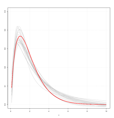
Let us now turn to a more interesting example of variance-mean mixtures. We take $X=T+W_{T}$ and choose $T$ to follow a Gamma distribution with the density $p_{T}(x)=x\exp(-x),$ $x\geq 0.$ The estimate (17) is constructed as follows. First note that $\psi(\lambda)=-\mathrm{i}\lambda+\lambda^{2}/2.$ In order to numerically compute the function $\Phi_{n}(1-z,X_{k})$ for $z=\gamma+\mathrm{i}v$ with $\gamma<1,$ we use the decomposition

(27) $$\frac{1}{n}\sum_{k=1}^{n}\Phi_{n}(1-z,X_{k}) =\int_{0}^{A_{n}}\left[\psi(\lambda)\right]^{-z}[\phi_{n}(\lambda)-e^{-m_{n}\psi(\lambda)}]\psi^{\prime}(\lambda)\,d\lambda$$

$$+m_{n}^{z-1}\Gamma(1-z)+O\bigl{(}m_{n}^{-(1-\gamma)}\exp(-m_{n}A_{n}^{2}/2)\bigr{)},$$

where $\phi_{n}(\lambda)=\frac{1}{n}\sum_{k=1}^{n}e^{\mathrm{i}\lambda X_{k}}$ is the empirical characteristic function and $m_{n}=\frac{1}{n}\sum_{k=1}^{n}X_{k}\to 2.$ This decomposition follows from a Cauchy argument similar as in the proof of Proposition 3.2 and is quite useful to reduce the cost of computing the integral in (27), since the integral on the r.h.s. of (27) is much easier to compute due to the asymptotic relation $\phi_{n}(\lambda)-e^{-m_{n}\psi(\lambda)}=O(\lambda^{2}),$ $\lambda\to 0.$ Next we take $\gamma=0.7,$ $A_{n}$ and $h_{n}$ as in Theorem 3.4 with $\varepsilon=0.5$ and $\beta=\pi/2$ (see Example 2.4). Figure 3 shows the performance of the estimate defined in (17): on the left-hand side $20$ independent realizations of the estimate $p_{T,n}$ for $n=1000$ are shown together with the true density $p_{T}.$ The box plots of the loss $\sup_{x\in[0,10]}\bigl{\{}|p_{T,n}(x)-p_{T}(x)|\bigr{\}}$ based on $100$ runs of the algorithm are depicted on the right-hand side of Figure 3. By comparing the right-hand sides of Figure 2 and Figure 3, we observe that the performances of the estimates (17) and (5) are similar, although the estimate (5) seem to have higher variance. This supports the claim of Theorem 3.4 about the same convergence rates in statistical Skorohod embedding and generalized statistical Skorohod embedding problems, given that $p_{T}\in\mathcal{C}(\beta,\gamma,L).$

Figure 3: Left: the Gamma density (red) and its $20$ estimates (grey) for the sample size $n=5000$. Right: the box plots of the loss $\sup_{x\in[0,10]}\bigl{\{}|p_{T,n}(x)-p_{T}(x)|\bigr{\}}$ for different sample sizes.

6 Proofs

6.1 Proof of Theorem 2.2

First let us estimate the bias of $p_{T,n}.$ We have

$$\mathbb{E}[p_{T,n}(x)] =\frac{1}{\sqrt{\pi}}\int_{-\infty}^{\infty}x^{-\gamma-\mathrm{i}v}K(vh_{n})\frac{\mathcal{M}[p_{|X|}](2(\gamma+\mathrm{i}v)-1)}{2^{\gamma+\mathrm{i}v}\Gamma(\gamma-1/2+\mathrm{i}v)}\,dv$$

$$=\frac{1}{2\pi}\int_{-1/h_{n}}^{1/h_{n}}x^{-\gamma-\mathrm{i}v}\mathcal{M}[p_{T}](\gamma+\mathrm{i}v)\,dv.$$

Hence

$$p_{T}(x)-\mathbb{E}[p_{T,n}(x)]=\frac{1}{2\pi}\int_{\{\left|v\right|\geq 1/h_{n}\}}\mathcal{M}[p_{T}](\gamma+\mathrm{i}v)x^{-\gamma-\mathrm{i}v}dv$$

and we then have the estimate,

$$\sup_{x\geq 0}\bigl{\{}x^{\gamma}|\mathbb{E}[p_{T,n}(x)]-p_{T}(x)|\bigr{\}} \leq\frac{1}{2\pi}\int_{\{\left|v\right|\geq 1/h_{n}\}}\left|\mathcal{M}[p_{T}](\gamma+\mathrm{i}v)\right|dv$$

$$\leq\frac{e^{-\beta/h_{n}}}{2\pi}\int_{\{\left|v\right|\geq 1/h_{n}\}}e^{-\beta\left|v\right|}\left|\mathcal{M}[p_{T}](\gamma+\mathrm{i}v)\right|e^{\beta\left|v\right|}dv$$

(28) $$\leq L\,\frac{e^{-\beta/h_{n}}}{2\pi}.$$

As to the variance, by the simple inequality $\operatorname{Var}\left(\int f_{t}dt\right)\leq\left(\int\sqrt{\operatorname{Var}[f_{t}]}dt\right)^{2},$ which holds for any random function $f_{t}$ with $\int\mathbb{E}[f^{2}_{t}]dt<\infty,$ we get

$$\operatorname{Var}[x^{\gamma}p_{T,n}(x)] =\operatorname{Var}\left[\frac{1}{\sqrt{\pi}}\int_{-\infty}^{\infty}x^{-\mathrm{i}v}K(vh_{n})\frac{\mathcal{M}_{n}[p_{|X|}](2(\gamma+\mathrm{i}v)-1)}{2^{\gamma+iv}\Gamma(\gamma-1/2+\mathrm{i}v)}\,dv\right]$$

$$\leq\frac{1}{\pi 2^{2\gamma}}\left[\int_{-1/h_{n}}^{1/h_{n}}\frac{\sqrt{\operatorname{Var}\left(\mathcal{M}_{n}[p_{|X|}](2(\gamma+\mathrm{i}v)-1)\right)}}{\left|\Gamma(\gamma-1/2+\mathrm{i}v)\right|}dv\right]^{2}\,$$

$$\leq\frac{1}{2n\pi}\left[\int_{-1/h_{n}}^{1/h_{n}}\frac{\sqrt{\operatorname{Var}\bigl{(}|X|^{2(\gamma+\mathrm{i}v-1)}\bigr{)}}}{\left|\Gamma(\gamma-1/2+\mathrm{i}v)\right|}dv\right]^{2}\,$$

(29) $$\leq\frac{1}{2n\pi}\left[\int_{-1/h_{n}}^{1/h_{n}}\frac{\sqrt{\mathbb{E}\left[|W_{T}|^{4(\gamma-1)}\right]}}{\left|\Gamma(\gamma-1/2+\mathrm{i}v)\right|}\,dv\right]^{2}.$$

Note that

$$\mathbb{E}\left[|W_{T}|^{4(\gamma-1)}\right] =\int_{0}^{\infty}\mathbb{E}\left[|W_{t}|^{4(\gamma-1)}\right]p_{T}(t)\,dt$$

$$=\mathbb{E}\left[|W_{1}|^{4(\gamma-1)}\right]\int_{0}^{\infty}t^{2(\gamma-1)}p_{T}(t)\,dt$$

$$=:C_{2}(\gamma)<\infty,$$

due to (6). We obtain from (29) due to Corollary 7.4 (see Appendix) and by taking into account (6),

$$\operatorname{Var}[x^{\gamma}p_{T,n}(x)]\leq\frac{C_{2}(\gamma)}{2n\pi}C_{3}h_{n}^{2\left(\gamma-1\right)}e^{\pi/h_{n}}=\frac{C_{3}(\gamma)}{n}h_{n}^{2\left(\gamma-1\right)}e^{\pi/h_{n}}.$$

and so (7) follows with $C_{\gamma,L}=\max(C_{3}(\gamma),\frac{L^{2}}{4\pi^{2}}).$ Finally, by plugging (8) into (7) we get (9) and the proof is finished.

6.2 Proof of Theorem  2.6

The proof is analog to the one of Theorem 2.2 , the only difference is the bias estimate (28) that now becomes

$$\sup_{x\geq 0}\bigl{\{}x^{\gamma}|\mathbb{E}[p_{T,n}(x)]-p_{T}(x)|\bigr{\}}\leq\frac{L}{2\pi}h_{n}^{\beta},$$

which gives (10) with a constant $D_{\gamma,L}=$ $\max(C_{3}(\gamma),\frac{L^{2}}{4\pi^{2}})$ again. Next with the choice (11) we obtain from (10) the logarithmic rate (13).

6.3 Proof of Theorem 2.8

Our construction relies on the following basic result (see [13] for the proof).

Theorem 6.1.

Suppose that for some $\varepsilon>0$ and $n\in\mathbb{N}$ there are two densities $p_{0,n},p_{1,n}\in\mathcal{G}$ such that

$$d(p_{0,n},p_{1,n})>2\varepsilon v_{n}.$$

If the observations in model $n$ follow the product law $\mathsf{P}_{p,n}=\mathsf{P}_{p}^{\otimes n}$ under the density $p\in\mathcal{G}$ and

$$\chi^{2}(p_{1,n}\,|\,p_{0,n})\leq n^{-1}\log(1+(2-4\delta)^{2})$$

holds for some $\delta\in(0,1/2)$, then the following lower bound holds for all density estimators $\hat{p}_{n}$ based on observations from model $n$:

$$\inf_{\hat{p}_{n}}\sup_{p\in\mathcal{G}}\operatorname{P}^{\otimes n}_{p}\big{(}d(\hat{p}_{n},p)\geq\varepsilon v_{n}\big{)}\geq\delta.$$

If the above holds for fixed $\varepsilon,\delta>0$ and all $n\in\mathbb{N}$, then the optimal rate of convergence in a minimax sense over $\mathcal{G}$ is not faster than $v_{n}$.

6.3.1 Proof of a lower bound for the class $\mathcal{C}(\beta,\gamma,L)$

Let us start with the construction of the densities $p_{0,n}$ and $p_{1,n}.$ Define for any $\nu>1$ and $M>0$ two auxiliary functions

$$q(x)=\frac{\nu\sin(\pi/\nu)}{\pi}\frac{1}{1+x^{\nu}},\quad x\geq 0$$

and

$$\rho_{M}(x)=\frac{1}{\sqrt{2\pi}}e^{-\frac{\log^{2}(x)}{2}}\frac{\sin(M\log(x))}{x},\quad x\geq 0.$$

The properties of the functions $q$ and $\rho_{M}$ are collected in the following lemma.

Lemma 6.2.

The function $q$ is a probability density on $\mathbb{R}_{+}$ with the Mellin transform

$$\mathcal{M}[q](z)=\frac{\sin(\pi/\nu)}{\sin(\pi z/\nu)},\quad\mathsf{Re}[z]>0.$$

The Mellin transform of the function $\rho_{M}$ is given by

(30) $$\mathcal{M}[\rho_{M}](u+\mathrm{i}v)=\frac{1}{2}\left[e^{(u-1+\mathrm{i}(v+M))^{2}/2}-e^{(u-1+\mathrm{i}(v-M))^{2}/2}\right].$$

Hence

$$\int_{0}^{\infty}\rho_{M}(x)dx=\mathcal{M}[\rho_{M}](1)=0.$$

Set now for any $M>0$

$$q_{0,M}(x):=q(x),\quad q_{1,M}(x):=q(x)+(q\vee\rho_{M})(x),$$

where $f\vee g$ stands for the multiplicative convolution of two functions $f$ and $g$ on $\mathbb{R}_{+}$ defined as

$$(f\vee g)(x):=\int_{0}^{\infty}\frac{f(t)g(x/t)}{t}dt,\quad x\geq 0.$$

The following lemma describes some properties of $q_{0,M}$ and $q_{1,M}.$

Lemma 6.3.

For any $M>0$ the function $q_{1,M}$ is a probability density satisfying

$$\|q_{0,M}-q_{1,M}\|_{\infty}=\sup_{x\in\mathbb{R}_{+}}|q_{0,M}(x)-q_{1,M}(x)|\gtrsim\exp(-M\pi/\nu),\quad M\to\infty.$$

Moreover, $q_{0,M}$ and $q_{1,M}$ are in $\mathcal{C}(\beta,\gamma,L)$ for all $0<\beta<\pi/\nu$ and $\gamma>0$ with $L$ depending on $\gamma.$

Proof.

First note that

$$\int_{0}^{\infty}q_{1,M}(x)dx=1+\int_{0}^{\infty}(q\vee\rho_{M})(x)=1+\mathcal{M}[q](1)\mathcal{M}[\rho_{M}](1)=1.$$

Furthermore, due to the Parseval identity

$$(q\vee\rho_{M})(y) = \int_{0}^{\infty}\frac{1}{\sqrt{2\pi}}e^{-\frac{\log^{2}(x)}{2}}\frac{\sin(M\log(x))}{x^{2}}\frac{1}{1+(y/x)^{\nu}}dx$$

$$= \int_{-\infty}^{\infty}\frac{1}{\sqrt{2\pi}}e^{-\frac{v^{2}}{2}}\sin(Mv)\frac{e^{-v}}{1+e^{-\nu(v-y_{l})}}dv$$

$$= e^{-\log(y)}\int_{-\infty}^{\infty}\frac{1}{\sqrt{2\pi}}e^{-\frac{v^{2}}{2}}\sin(Mv)\frac{e^{(y_{l}-v)}}{1+e^{\nu(\log(y)-v)}}dv$$

$$= \frac{e^{-\log(y)}}{2\pi}\int_{-\infty}^{\infty}\frac{1}{\sqrt{2\pi}}e^{-\frac{v^{2}}{2}}\sin(Mv)\frac{e^{(\log(y)-v)}}{1+e^{\nu(\log(y)-v)}}dv$$

$$= \frac{e^{-\log(y)}}{2\pi}\int_{-\infty}^{\infty}e^{-\mathrm{i}u\log(y)}\left[\frac{H(u+M)-H(u-M)}{2}\right]\mathcal{F}[R](u)du,$$

where $R(x)=\frac{e^{x}}{1+e^{\nu x}}$ and $H(x)=e^{-x^{2}/2}$. Note that

$$\mathcal{F}[R](u)=\int_{-\infty}^{\infty}\frac{e^{x+\mathrm{i}ux}}{1+e^{\nu x}}\,dx=\frac{1}{\nu}\int_{-\infty}^{\infty}\frac{e^{v/\nu+\mathrm{i}uv/\nu}}{1+e^{v}}\,dx=\frac{1}{\nu}\,\Gamma\left(\frac{1+\mathrm{i}u}{\nu}\right)\Gamma\left(1-\frac{1+\mathrm{i}u}{\nu}\right).$$

Hence due to (56)

$$\sup_{y\in\mathbb{R}_{+}}|q_{0,M}(y)-q_{1,M}(y)|=\sup_{y\in\mathbb{R}_{+}}|(q\vee\rho_{M})(y)|\gtrsim\exp(-M\pi/\nu),\quad M\to\infty.$$

The second statement of the lemma follows from Lemma 6.2 and the fact that $\mathcal{M}[q\vee\rho_{M}]=\mathcal{M}[q]\mathcal{M}[\rho_{M}].$ ∎

Let $T_{0,M}$ and $T_{1,M}$ be two random variables with densities $q_{0,M}$ and $q_{1,M},$ respectively. Then the density of the r.v. $|W_{T_{i,M}}|,$ $i=0,1,$ is given by

$$p_{i,M}(x) :=\frac{2}{\sqrt{2\pi}}\int_{0}^{\infty}\lambda^{-1/2}e^{-\frac{x^{2}}{2\lambda}}q_{i,M}(\lambda)\,d\lambda\quad i=0,1.$$

For the Mellin transform of $p_{i,M}$ we get

$$\mathcal{M}[p_{i,M}](z) =\mathbb{E}\bigl{[}|W_{1}|^{z-1}\bigr{]}\mathbb{E}\bigl{[}T_{i,M}^{(z-1)/2}\bigr{]}$$

$$=\mathbb{E}\bigl{[}|W_{1}|^{z-1}\bigr{]}\mathcal{M}[q_{i,M}]((z+1)/2)$$

(31) $$=\frac{2^{z/2}}{\sqrt{2\pi}}\Gamma(z/2)\mathcal{M}[q_{i,M}]((z+1)/2),\quad i=0,1.$$

Lemma 6.4.

The $\chi^{2}$-distance between the densities $p_{0,M}$ and $p_{1,M}$ fulfills

$$\chi^{2}(p_{1,M}|p_{0,M})=\int\frac{(p_{1,M}(x)-p_{0,M}(x))^{2}}{p_{0,M}(x)}dx\lesssim e^{-M\pi(1+2/\nu)},\quad M\to\infty.$$

Proof.

First note that $p_{0,M}(x)>0$ on $[0,\infty).$ Since

$$p_{0,M}(x) = \frac{2}{\sqrt{2\pi}}\frac{\nu\sin(\pi/\nu)}{\pi}\int_{0}^{\infty}\lambda^{-1/2}e^{-\frac{x^{2}}{2\lambda}}\frac{1}{1+\lambda^{\nu}}d\lambda$$

$$/y=1/\lambda/ = \frac{2}{\sqrt{2\pi}}\frac{\nu\sin(\pi/\nu)}{\pi}\int_{0}^{\infty}y^{1/2}e^{-y\frac{x^{2}}{2}}\frac{1}{y^{2}(1+y^{-\nu})}dy$$

$$= \frac{2}{\sqrt{2\pi}}\frac{\nu\sin(\pi/\nu)}{\pi}\int_{0}^{\infty}e^{-y\frac{x^{2}}{2}}\frac{y^{\nu-1/2-1}}{(1+y^{\nu})}dy$$

$$\asymp \frac{2}{\sqrt{2\pi}}\frac{\nu\sin(\pi/\nu)}{\pi}\Gamma(\nu-1/2)x^{-2\nu+1},\quad x\to\infty,$$

we have $p_{0,M}(x)\gtrsim x^{-2\nu+1},$ $x\to\infty.$ Furthermore, due to (6.3.1) and the Parseval identity

(32) $$\int_{0}^{\infty}x^{2\nu-1}\left|p_{0,M}(x)-p_{1,M}(x)\right|^{2}dx=\\ \frac{2^{-4+2\nu}}{\pi}\int_{\gamma-i\infty}^{\gamma+i\infty}\mathcal{M}[q\vee\rho_{M}]\left(\frac{z+1}{2}\right)\Gamma\left(\frac{z}{2}\right)\mathcal{M}[q\vee\rho_{M}]\left(\frac{2\nu-z+1}{2}\right)\Gamma\left(\frac{2\nu-z}{2}\right)dz,$$

where $\mathcal{M}[q\vee\rho_{M}](z)=\mathcal{M}[q](z)\mathcal{M}[\rho_{M}](z).$ Due to (30)

(33) $$|\mathcal{M}[\rho_{M}](u+\mathrm{i}v)|\leq e^{\frac{(u-1)^{2}}{2}}\frac{\phi(v+M)+\phi(v-M)}{2}$$

with $\phi(v)=e^{-\frac{v^{2}}{2}}.$ Combining (56) (Appendix), (32) and (33), we derive

$$\chi^{2}(p_{1,M}|p_{0,M}) = \int\frac{(p_{1,M}(x)-p_{0,M}(x))^{2}}{p_{0,M}(x)}dx$$

$$\lesssim \int_{0}^{\infty}(p_{1,M}(x)-p_{0,M}(x))^{2}dx+\int_{0}^{\infty}x^{2\nu-1}(p_{1,M}(x)-p_{0,M}(x))^{2}dx$$

$$\lesssim \int_{-\infty}^{\infty}|v|^{\nu-1}e^{-|v|\pi/2-|v|\pi/\nu}\left(\phi(v/2+M)+\phi(v/2-M)\right)^{2}dv$$

$$\lesssim M^{\nu-1}e^{-M\pi(1+2/\nu)},\quad M\to\infty.$$

∎

Fix some $\kappa\in(0,1/2).$ Due to Lemma 6.4, the inequality

$$n\chi^{2}(p_{1,M}|p_{0,M})\leq\kappa$$

holds for $M$ large enough, provided

$$M=\frac{1+\varepsilon}{\pi(1+2/\nu)}(\log(n)+(\nu-1)\log\log(n))$$

for arbitrary small $\varepsilon>0.$ Hence Lemma 6.3 and Theorem 6.1 imply

$$\inf_{\hat{p}_{n}}\sup_{p\in\mathcal{C}(\beta,\gamma,L)}\mathsf{P}_{p,n}\big{(}\|\hat{p}_{n}-p\|_{\infty}\geq cv_{n}\big{)}\geq\delta.$$

for any $\beta<\pi/\nu<\pi,$ any $\gamma>0,$ some constants $c>0,$ $\delta>0$ and $v_{n}=n^{-\beta/(\pi+2\beta)}\log^{-\frac{\pi-\beta}{\pi+2\beta}}(n).$

6.3.2 Proof of a lower bound for the class $\mathcal{D}(\beta,\gamma,L)$

Define for any $\nu>1,$ $\alpha>0$ and $M>0,$

$$q(x)=\left[2\Gamma(\nu)\right]^{-1}\times\begin{cases}\log^{\nu-1}(1/x),&0\leq x\leq 1,\\ x^{-2}\log^{\nu-1}(x),&x>1\end{cases}$$

and

$$\rho_{M}(x)=\frac{1}{\sqrt{2\pi}}e^{-\frac{\log^{2}(x)}{2}}\frac{\sin(M\log(x))}{x\log(x)},\quad x\geq 0.$$

The properties of the functions $q$ and $\rho_{M}$ can be found in the next lemma.

Lemma 6.5.

The function $q$ is a probability density on $\mathbb{R}_{+}$ with the Mellin transform

$$\mathcal{M}[q](z)=\frac{1}{2}\left[z^{-\nu}+(2-z)^{-\nu}\right],\quad 0<\mathsf{Re}[z]<2.$$

The Mellin transform of the function $\rho_{M}$ is given by

(34) $$\mathcal{M}[\rho_{M}](u+\mathrm{i}v)=e^{\frac{(u-1)^{2}}{2}}\frac{G(u,v+M)-G(u,v-M)}{2},$$

where $G(u,v)=\int_{-\infty}^{v}e^{-\frac{x^{2}}{2}+\mathrm{i}x(u-1)}dx.$ Hence

$$\zeta_{M}:=\int_{0}^{\infty}\rho_{M}(x)dx=\mathcal{M}[\rho_{M}](1)=\int_{-M}^{M}e^{-\frac{x^{2}}{2}}dx.$$

Set now for any $M>0$

$$q_{0,M}(x):=q(x),\quad q_{1,M}(x):=(1-\zeta_{M})q(x)+(q\vee\rho_{M})(x),$$

where $f\vee g$ stands for the multiplicative convolution of two functions $f$ and $g$ on $\mathbb{R}_{+}$ defined via

$$(f\vee g)(x):=\int_{0}^{\infty}\frac{f(t)g(x/t)}{t}dt.$$

Lemma 6.6.

For any $M>0,$ the function $q_{1,M}$ is a probability density satisfying

$$\sup_{x\in(1-\delta,1+\delta)}|q_{0,M}(x)-q_{1,M}(x)|\asymp|\cos(\pi\nu/2)|M^{-\nu+1},\quad M\to\infty,$$

where $\delta>0$ is a fixed number. Moreover, $q_{0,M}$ and $q_{1,M}$ are in $\mathcal{D}(\beta,\gamma,L)$ for all $\beta<\nu-1$ and $\gamma\in(0,2).$

Proof.

First note that

$$\int_{0}^{\infty}q_{1,M}(x)dx=1+\int_{0}^{\infty}(q\vee\rho_{M})(x)-\zeta_{M}=1+\mathcal{M}[\rho_{M}](1)\times\mathcal{M}[q](1)-\zeta_{M}=1.$$

Furthermore, $(q\vee\rho_{M})(y)=\left[2\Gamma(\nu)\right]^{-1}[I_{1}(y)+I_{2}(y)]$ with

$$I_{1}(y) = \int_{y}^{\infty}e^{-\frac{\log^{2}(x)}{2\alpha}}x^{-2}\frac{\sin(M\log(x))}{\log(x)}\log^{\nu-1}(x/y)dx$$

$$= \int_{\log(y)}^{\infty}e^{-\frac{z^{2}}{2\alpha}-z}\frac{\sin(Mz)}{z}(z-\log(y))^{\nu-1}dz$$

and

$$I_{2}(y) = \int_{0}^{y}e^{-\frac{\log^{2}(x)}{2\alpha}}y^{-2}\frac{\sin(M\log(x))}{\log(x)}\log^{\nu-1}(y/x)dx$$

$$= \int_{-\infty}^{\log(y)}e^{-\frac{z^{2}}{2\alpha}+z}y^{-2}\frac{\sin(Mz)}{z}(\log(y)-z)^{\nu-1}dz.$$

By taking $y=\exp(A),$ we get for $I_{1}(y)$

$$I_{1}(y) = \int_{0}^{\infty}e^{-\frac{(z+A)^{2}}{2\alpha}-(z+A)}\frac{\sin(M(z+A))}{z+A}z^{\nu-1}dz$$

$$= \cos(AM)\int_{0}^{\infty}\frac{e^{-\frac{(z+A)^{2}}{2\alpha}-(z+A)}}{z+A}\sin(Mz)z^{\nu-1}dz$$

$$+\sin(AM)\int_{0}^{\infty}\frac{e^{-\frac{(z+A)^{2}}{2\alpha}-(z+A)}}{z+A}\cos(Mz)z^{\nu-1}dz.$$

The well known Erdélyi lemma implies

$$\int_{0}^{\infty}\frac{e^{-\frac{(z+A)^{2}}{2\alpha}-(z+A)}}{z+A}\sin(Mz)z^{\nu-1}dz\asymp\frac{e^{-\frac{A{}^{2}}{2\alpha}-A}}{A}\Gamma(\nu)\sin(\pi\nu/2)M^{-\nu},\quad M\to\infty$$

and

$$\int_{0}^{\infty}\frac{e^{-\frac{(z+A)^{2}}{2\alpha}-(z+A)}}{z+A}\cos(Mz)z^{\nu-1}dz\asymp\frac{e^{-\frac{A{}^{2}}{2\alpha}-A}}{A}\Gamma(\nu)\cos(\pi\nu/2)M^{-\nu},\quad M\to\infty.$$

Hence

(35) $$I_{1}(e^{A})\asymp\frac{e^{-\frac{A{}^{2}}{2\alpha}-A}}{A}\Gamma(\nu)\sin(AM+\pi\nu/2)M^{-\nu},M\to\infty.$$

Analogously

$$I_{2}(e^{A}) = e^{-2A}\int_{-\infty}^{A}e^{-\frac{z^{2}}{2\alpha}+z}\frac{\sin(Mz)}{z}(A-z)^{\nu-1}dz$$

$$= e^{-2A}\int_{0}^{\infty}e^{-\frac{(A-z)^{2}}{2\alpha}+A-z}\frac{\sin(M(A-z))}{A-z}z{}^{\nu-1}dz$$

$$= e^{-2A}\sin(AM)\int_{0}^{\infty}e^{-\frac{(A-z)^{2}}{2\alpha}+A-z}\frac{\cos(Mz)}{A-z}z{}^{\nu-1}dz$$

$$-e^{-2A}\cos(AM)\int_{0}^{\infty}e^{-\frac{(A-z)^{2}}{2\alpha}+A-z}\frac{\sin(Mz)}{A-z}z{}^{\nu-1}dz$$

$$\asymp \frac{e^{-\frac{A^{2}}{2\alpha}-A}}{A}\Gamma(\nu)\sin(AM-\pi\nu/2)M^{-\nu}.$$

Combining the previous estimates, we arrive at

$$I_{2}(e^{A})+I_{1}(e^{A})=2\frac{e^{-\frac{A^{2}}{2\alpha}-A}}{A}\Gamma(\nu)\sin(AM)\cos(\pi\nu/2)M^{-\nu}.$$

It remains to note that the maximum of r.h.s of (35) is attained for $A\in\{\pi/2M,3\pi/2M\}$ and

$$\sup_{A}[I_{2}(e^{A})+I_{1}(e^{A})]\asymp\Gamma(\nu)|\cos(\pi\nu/2)|M^{-\nu+1}.$$

The property $q_{1,M}\in\mathcal{D}(\beta,\gamma,L)$ for all $\beta<\nu-1$ and $\gamma\in(0,2)$ with $L$ depending on $\gamma,$ follows from the identity $\mathcal{M}[q_{1,M}](z)=\mathcal{M}[q](z)(1-\zeta_{M})+\mathcal{M}[\rho_{M}](z)\mathcal{M}[q](z)$ and (34). ∎

Let $T_{0,M}$ and $T_{1,M}$ be two random variables with densities $q_{0,M}$ and $q_{1,M}$ respectively. The the density of the r.v. $|W_{T_{i,M}}|,$ $i=0,1,$ is given by

$$p_{i,M}(x) :=\frac{2}{\sqrt{2\pi}}\int_{0}^{\infty}\lambda^{-1/2}e^{-\frac{x^{2}}{2\lambda}}q_{i,M}(\lambda)d\lambda,\quad i=0,1.$$

For the Mellin transform of $p_{i,M},$ we have

$$\mathcal{M}[p_{i,M}](z) =\mathbb{E}\bigl{[}|W_{1}|^{z-1}\bigr{]}\mathbb{E}\bigl{[}T_{i,M}^{(z-1)/2}\bigr{]}$$

$$=\mathbb{E}\bigl{[}|W_{1}|^{z-1}\bigr{]}\mathcal{M}[q_{i,M}]((z+1)/2)$$

(36) $$=\frac{2^{z/2}}{\sqrt{2\pi}}\Gamma(z/2)\mathcal{M}[q_{i,M}]((z+1)/2).$$

Lemma 6.7.

The $\chi^{2}$-distance between the densities $p_{0,M}$ and $p_{1,M}$ satisfies

$$\chi^{2}(p_{1,M}|p_{0,M}):=\int\frac{(p_{1,M}(x)-p_{0,M}(x))^{2}}{p_{0,M}(x)}dx\lesssim e^{-M\pi/2},\quad M\to\infty.$$

Proof.

First note that $p_{0,M}(x)>0$ on $[0,\infty).$ Since

$$\int_{0}^{1}\lambda^{-1/2}e^{-\frac{x^{2}}{2\lambda}}\log^{\nu-1}(1/\lambda)d\lambda = \int_{0}^{1}\lambda^{-1/2}e^{-\frac{x^{2}}{2\lambda}}\log^{\nu-1}(1/\lambda)d\lambda$$

$$/y=1/\lambda,\lambda=1/y/ = \int_{1}^{\infty}y^{-3/2}e^{-x^{2}y/2}\log^{\nu-1}(y)dy$$

$$= \int_{x^{2}}^{\infty}x^{-2}(y/x^{2})^{-3/2}e^{-y/2}\log^{\nu-1}(y/x^{2})dy$$

$$= x\int_{x^{2}}^{\infty}y{}^{-3/2}e^{-y/2}\log^{\nu-1}(y/x^{2})dy\lesssim e^{-x^{2}/2}$$

and

$$\int_{1}^{\infty}\lambda^{-3/2}e^{-\frac{x^{2}}{2\lambda}}\log^{\nu-1}(\lambda)d\lambda = \int_{0}^{1}y^{-1/2}e^{-\frac{x^{2}}{2}y}\log^{\nu-1}(1/y)dy$$

$$\asymp \frac{\Gamma(1/2)}{\sqrt{2}}x^{-1}\log^{\nu-1}(x^{2}).$$

we have $p_{0,M}(x)\gtrsim x^{-1},$ $x\to\infty.$ Furthermore, due to (6.3.2) and the Parseval identity

(37) $$\int_{0}^{\infty}x^{a-1}\left|p_{0,M}(x)-p_{1,M}(x)\right|^{2}dx=\\ \frac{2^{-4+a}}{\pi}\int_{\gamma-\mathrm{i}\infty}^{\gamma+\mathrm{i}\infty}\mathcal{M}[q\vee\rho_{M}]\left(\frac{z+1}{2}\right)\Gamma\left(\frac{z}{2}\right)\mathcal{M}[q\vee\rho_{M}]\left(\frac{a-z+1}{2}\right)\Gamma\left(\frac{a-z}{2}\right)dz,$$

where $\mathcal{M}[q\vee\rho_{M}](z)=\mathcal{M}[q](z)\mathcal{M}[\rho_{M}](z).$ Due to (34)

(38) $$|\mathcal{M}[\rho_{M}](u+\mathrm{i}v)|\leq e^{\frac{(u-1)^{2}}{2}}\frac{\Phi(v+M)+\Phi(v-M)}{2}$$

with $\Phi(v)=\int_{-\infty}^{v}e^{-\frac{x^{2}}{2}}dx.$ Combining (37) with properly chosen $\gamma>0$, (38) and Lemma  7.3 (see Appendix), we derive

$$\chi^{2}(p_{1}|p_{0}) = \int\frac{(p_{1}(x)-p_{0}(x))^{2}}{p_{0}(x)}dx\lesssim\int_{0}^{\infty}(p_{1}(x)-p_{0}(x))^{2}dx+\int_{0}^{\infty}x(p_{1}(x)-p_{0}(x))^{2}dx$$

$$\lesssim \int_{-\infty}^{\infty}e^{-|v|\pi/2}\left(\Phi(v/2+M)+\Phi(v/2-M)\right)^{2}dv\lesssim e^{-M\pi/2},\quad M\to\infty.$$

∎

Fix some $\kappa\in(0,1/2).$ Due to Lemma 6.7, the inequality

$$n\chi^{2}(p_{1,M}|p_{0,M})\leq\kappa$$

holds for $M$ large enough, provided

$$M=\frac{2(1+\varepsilon)}{\pi}\log(n)$$

for arbitrary small $\varepsilon>0.$ Hence Lemma 6.6 and Theorem 6.1 imply

$$\inf_{\hat{p}_{n}}\sup_{p\in\mathcal{D}(\beta,\gamma,L)}\mathsf{P}_{p,n}\big{(}\|\hat{p}_{n}-p\|_{\infty}\geq cv_{n}\big{)}\geq\delta.$$

for any $\beta<\nu-1,$ any $\gamma\in(0,2),$ some constants $c>0,$ $\delta>0$ and $v_{n}=\log^{-\beta}(n).$

6.4 Proof of Proposition 2.3

It holds

$$p_{T,n}(x)-\mathbb{E}[p_{T,n}(x)] =\frac{1}{\sqrt{\pi}}\int_{-1/h_{n}}^{1/h_{n}}x^{-\gamma-\mathrm{i}v}\frac{K(vh_{n})}{2^{\gamma+\mathrm{i}v}}$$

$$\times\frac{\bigl{\{}\mathcal{M}_{n}[p_{|X|}](2(\gamma+\mathrm{i}v)-1)-\mathcal{M}[p_{|X|}](2(\gamma+\mathrm{i}v)-1)\bigr{\}}}{\Gamma((\gamma+\mathrm{i}v)-1/2)}\,dv.$$

Due to Proposition 7.1

$$\sup_{x\geq 0}\bigl{\{}x^{\gamma}|\mathbb{E}[p_{T,n}(x)]-p_{T}(x)|\bigr{\}}\leq\frac{\Delta_{n}}{\sqrt{\pi n}}\int_{-1/h_{n}}^{1/h_{n}}\frac{A_{1}}{2^{\gamma}}\frac{\log(e+|v|)}{\Gamma((\gamma+\mathrm{i}v)-1/2)}\,dv$$

with $\Delta_{n}=O_{a.s.}(1).$

6.5 Proof of Proposition 2.9

We have

$$\operatorname{Var}(Z_{n,1}) =\frac{1}{\pi}\int_{-1/h_{n}}^{1/h_{n}}\int_{-1/h_{n}}^{1/h_{n}}\frac{x^{-2\gamma-{\mathrm{i}}(v-u)}}{2^{2\gamma+{\mathrm{i}}(v-u)}}\frac{\operatorname{Cov}\left(|X_{1}|^{2(\gamma+{\mathrm{i}}v-1)},|X_{1}|^{2(\gamma+{\mathrm{i}}u-1)}\right)}{2^{2\gamma+{\mathrm{i}}(v-u)}\Gamma(\gamma-1/2+{\mathrm{i}}v)\Gamma(\gamma-1/2-{\mathrm{i}}u)}\,du\,dv$$

$$=\frac{1}{\pi}\int_{-1/h_{n}}^{1/h_{n}}\int_{-1/h_{n}}^{1/h_{n}}\frac{1}{\left(2x\right)^{2(\gamma-1)+{\mathrm{i}}(v-u)}}\frac{\mathcal{M}[p_{\left|X\right|}](4\gamma-3+2{\mathrm{i}}(v-u))}{\Gamma(\gamma-1/2+{\mathrm{i}}v)\Gamma(\gamma-1/2-{\mathrm{i}}u)}\,dv\,du$$

$$-\frac{1}{\pi}\left|\int_{-1/h_{n}}^{1/h_{n}}\frac{1}{\left(2x\right)^{(\gamma+{\mathrm{i}}v-1)}}\frac{\mathcal{M}[p_{\left|X\right|}](2\gamma-1+2{\mathrm{i}}v)}{\Gamma(\gamma-1/2+{\mathrm{i}}v)}\,dv\right|^{2}=R_{1}-R_{2}.$$

Note that

$$R_{2} \leq\frac{1}{(2x)^{2\left(\gamma-1\right)}}\left(\int_{-1/h_{n}}^{1/h_{n}}\left|\frac{\mathcal{M}[p_{\left|X\right|}](2\gamma-1+2{{\mathrm{i}}}v)}{\Gamma(\gamma-1/2+{{\mathrm{i}}}v)}\,\right|dv\right)^{2}$$

$$=\frac{1}{(2x)^{2\left(\gamma-1\right)}}\left|\int_{-1/h_{n}}^{1/h_{n}}\bigl{|}\mathcal{M}[p_{T}](\gamma+{{\mathrm{i}}}v)\bigr{|}\,dv\right|^{2}<C<\infty$$

and furthermore

$$R_{1} =\frac{1}{x^{2(\gamma-1)}\pi}\int_{-1/h_{n}}^{1/h_{n}}\int_{-1/h_{n}}^{1/h_{n}}\frac{1}{x^{{{\mathrm{i}}}(v-u)}}\frac{\Gamma(2\gamma-3/2+{{\mathrm{i}}}(v-u))\mathcal{M}[p_{T}](2\gamma-1+{{\mathrm{i}}}(v-u))}{\Gamma(\gamma-1/2+{{\mathrm{i}}}v)\Gamma(\gamma-1/2-{{\mathrm{i}}}u)}\,dv\,du$$

$$=\frac{1}{x^{2(\gamma-1)}\pi}\times I_{n}.$$

Without loss of generality we may take $x=1$ (for $x\neq 1$ the proof is similar). Observe that for $v\in\mathbb{R},$

(39) $$|\Gamma(\gamma-1/2+{{\mathrm{i}}}v)|\geq C_{1}1_{\left|v\right|\leq 2}+C_{2}1_{\left|v\right|>2}\left|v\right|^{\gamma-1}e^{-\pi\left|v\right|/2},$$

for some constants $C_{1}>0,$ $C_{2}>0$ (depending on $\gamma$), and that

(40) $$|\Gamma(2\gamma-3/2+{{\mathrm{i}}}(v-u))|\leq D_{1}1_{\left|u-v\right|\leq 2}+1_{\left|u-v\right|>2}D_{2}\left|u-v\right|^{2(\gamma-1)}e^{-\pi\left|u-v\right|/2}$$

for some $D_{1}>0,$ $D_{2}>0.$ Let $\rho_{n}=h_{n}^{-\alpha}$ for $0<\alpha<1/2$. By the estimates (39) and (40), one can straightforwardly derive that the integral

$$I_{1,n,\rho_{n}}:=\int_{-1/h_{n}}^{1/h_{n}}\int_{-1/h_{n}}^{1/h_{n}}1_{\left|v-u\right|\geq\rho_{n}}\frac{\Gamma(2\gamma-3/2+{{\mathrm{i}}}(v-u))\mathcal{M}[p_{T}](2\gamma-1+{{\mathrm{i}}}(v-u))}{\Gamma(\gamma-1/2+{{\mathrm{i}}}v)\Gamma(\gamma-1/2-{{\mathrm{i}}}u)}\,dv\,du$$

can be bounded from above as

$$|I_{1,n,\rho_{n}}|\lesssim h_{n}^{-3\left|1-\gamma\right|}e^{\pi\left(\frac{1}{2h_{n}}-\rho_{n}/2\right)}+h_{n}^{-2\left|1-\gamma\right|-1}e^{\pi\left(\frac{1}{h_{n}}-\rho_{n}/2\right)}+h_{n}^{-4\left|1-\gamma\right|-1}e^{\pi\left(\frac{1}{h_{n}}-\rho_{n}\right)}$$

for $n\rightarrow\infty.$ Similarly

$$\int_{-1/h_{n}}^{1/h_{n}}\int_{-1/h_{n}}^{1/h_{n}}1_{\left|u\right|\leq\frac{1}{h_{n}}-\rho_{n}}1_{\left|v-u\right|\leq\rho_{n}}\frac{\Gamma(2\gamma-3/2+{{\mathrm{i}}}(v-u))\mathcal{M}[p_{T}](2\gamma-1+{{\mathrm{i}}}(v-u))}{\Gamma(\gamma-1/2+{{\mathrm{i}}}v)\Gamma(\gamma-1/2-{{\mathrm{i}}}u)}\,dv\,du\\ =O\Bigl{(}h_{n}^{-l}e^{\pi\left(\frac{1}{h_{n}}-\rho_{n}\right)}\Bigr{)}$$

and

$$\int_{-1/h_{n}}^{1/h_{n}}\int_{-1/h_{n}}^{1/h_{n}}1_{\left|v\right|\leq\frac{1}{h_{n}}-\rho_{n}}1_{\left|v-u\right|\leq\rho_{n}}\frac{\Gamma(2\gamma-3/2+{{\mathrm{i}}}(v-u))\mathcal{M}[p_{T}](2\gamma-1+{{\mathrm{i}}}(v-u))}{\Gamma(\gamma-1/2+{{\mathrm{i}}}v)\Gamma(\gamma-1/2-{{\mathrm{i}}}u)}\,dv\,du\\ =O\Bigl{(}h_{n}^{-l}e^{\pi\left(\frac{1}{h_{n}}-\rho_{n}\right)}\Bigr{)}$$

for some $l>0.$ Hence

$$I_{2,n,\rho_{n}}:= \int_{-1/h_{n}}^{1/h_{n}}\int_{-1/h_{n}}^{1/h_{n}}1_{\left|v-u\right|\leq\rho_{n}}\frac{\Gamma(2\gamma-3/2+{{\mathrm{i}}}(v-u))\mathcal{M}[p_{T}](2\gamma-1+{{\mathrm{i}}}(v-u))}{\Gamma(\gamma-1/2+{{\mathrm{i}}}v)\Gamma(\gamma-1/2-{{\mathrm{i}}}u)}\,dv\,du$$

$$=\int_{-1/h_{n}}^{1/h_{n}}\int_{-1/h_{n}}^{1/h_{n}}1_{\left|u\right|\geq\frac{1}{h_{n}}-\rho_{n}}1_{\left|v\right|\geq\frac{1}{h_{n}}-\rho_{n}}1_{\left|v-u\right|\leq\rho_{n}}$$

$$\times\frac{\Gamma(2\gamma-3/2+{{\mathrm{i}}}(v-u))\mathcal{M}[p_{T}](2\gamma-1+{{\mathrm{i}}}(v-u))}{\Gamma(\gamma-1/2+{{\mathrm{i}}}v)\Gamma(\gamma-1/2-{{\mathrm{i}}}u)}\,dv\,du+O\Bigl{(}h_{n}^{-l}e^{\pi\left(\frac{1}{h_{n}}-\rho_{n}\right)}\Bigr{)}$$

$$=:I_{3,n,\rho_{n}}+O\Bigl{(}h_{n}^{-l}e^{\pi\left(\frac{1}{h_{n}}-\rho_{n}\right)}\Bigr{)}.$$

Now let us study the asymptotic behaviour of the integral $I_{3,n,\rho_{n}}.$ To this end, we will use the Stirling formula

$$\Gamma(\gamma-1/2+{{\mathrm{i}}}v)=\left(\gamma-1/2+iv\right)^{\gamma-1+iv}e^{-\gamma+1/2-iv}\sqrt{2\pi}(1+O(\left|v\right|^{-1})).$$

First consider the integrand of $I_{3,n,\rho_{n}}$ in the case $u,v\rightarrow+\infty,$ where

$$\Gamma(\gamma-1/2+{{\mathrm{i}}}v)\Gamma(\gamma-1/2-{{\mathrm{i}}}u) =2\pi\exp\left[iv\log v-iu\log u-i\left(v-u\right)\right]$$

$$\times\exp\left[-\frac{\pi}{2}\left(u+v\right)+\left(\gamma-1\right)\left(\log v+\log u\right)\right](1+O(1/u)+O(1/v)).$$

Then on the set

$$\left\{\left|u\right|\geq\frac{1}{h_{n}}-\rho_{n}\right\}\cap\left\{\left|v\right|\geq\frac{1}{h_{n}}-\rho_{n}\right\}\cap\left\{\left|v-u\right|\leq\rho_{n}\right\}\cap\left\{v\geq 0,u\geq 0\right\}$$

we define $u=1/h_{n}-r,$ $v=1/h_{n}-s$ with $0<r,s<\rho_{n},$ $\left|r-s\right|<\rho_{n}$ to get

$$\Gamma(\gamma-1/2+{{\mathrm{i}}}v)\Gamma(\gamma-1/2-{{\mathrm{i}}}u) =2e^{i\left(1/h_{n}-s\right)\log\left(1/h_{n}-s\right)-i\left(1/h_{n}-r\right)\log\left(1/h_{n}-r\right)-i\left(r-s\right)}$$

$$\times h_{n}^{-2\left(\gamma-1\right)}\exp\left[-\pi/h_{n}\right]\exp\left[(r+s)\pi\right]$$

$$\times(1+O(h_{n}))(1+O(\rho_{n}h_{n})).$$

Note that due to the choice of $\rho_{n},$ $\rho_{n}h_{n}\downarrow 0$ and $\rho_{n}^{2}h_{n}\downarrow 0.$ Using the asymptotic expansion

$$\left(1/h_{n}-s\right)\log\left(1/h_{n}-s\right)-\left(1/h_{n}-r\right)\log\left(1/h_{n}-r\right)-\left(r-s\right)=\left(r-s\right)\log\left(1/h_{n}\right)+O(\rho_{n}^{2}h_{n}),$$

we derive

$$\Gamma(\gamma-1/2+{{\mathrm{i}}}v)\Gamma(\gamma-1/2-{{\mathrm{i}}}u) =2\pi h_{n}^{-2\left(\gamma-1\right)}\exp\left[-\pi/h_{n}\right]\exp\left[(r+s)\pi\right]$$

$$\times\exp\left[i\left(r-s\right)\log\left(1/h_{n}\right)\right](1+O(\rho_{n}^{2}h_{n})).$$

Analogously, on the set

$$\left\{\left|u\right|\geq\frac{1}{h_{n}}-\rho_{n}\right\}\cap\left\{\left|v\right|\geq\frac{1}{h_{n}}-\rho_{n}\right\}\cap\left\{\left|v-u\right|\leq\rho_{n}\right\}\cap\left\{v\leq 0,u\leq 0\right\}$$

we define $u=-1/h_{n}+r,$ $v=-1/h_{n}+s,$ with $0<r,s<\rho_{n},$ $\left|r-s\right|<\rho_{n},$ to get

$$\Gamma(\gamma-1/2+{{\mathrm{i}}}v)\Gamma(\gamma-1/2-{{\mathrm{i}}}u) =2\pi h_{n}^{-2\left(\gamma-1\right)}\exp\left[-\pi/h_{n}\right]\exp\left[(r+s)\pi\right]$$

$$\times\exp\left[-i\left(r-s\right)\log\left(1/h_{n}\right)\right](1+O(\rho_{n}^{2}h_{n})).$$

Hence the integral $I_{3,n,\rho_{n}}$ can be decomposed as follows

$$I_{3,n,\rho_{n}}=:\frac{h_{n}^{2\left(\gamma-1\right)}}{\pi}\exp\left[\pi/h_{n}\right]\left\{\mathsf{Re}[I_{4,n,\rho_{n}}]+O(\rho_{n}^{2}h_{n})\right\},$$

where

$$I_{4,n,\rho_{n}} =\int\int 1_{0\leq r\leq\rho_{n}}1_{0\leq s\leq\rho_{n}}1_{\left|r-s\right|\leq\rho_{n}}\exp\left[-(r+s)\pi\right]\Gamma(2\gamma-3/2+{{\mathrm{i}}}(r-s))$$

$$\times\mathcal{M}[p_{T}](2\gamma-1+{{\mathrm{i}}}(r-s))\exp\left[i\left(s-r\right)\log\left(1/h_{n}\right)\right]drds$$

$$=\int_{0}^{\rho_{n}}e^{-2v\pi}R_{n}(v)dv$$

with

$$R_{n}(v)=\int 1_{0\leq u\leq\rho_{n}-v}e^{-u\pi}\Gamma(2\gamma-3/2+{{\mathrm{i}}}u)\mathcal{M}[p_{T}](2\gamma-1+{{\mathrm{i}}}u)e^{iu\log\left(1/h_{n}\right)}du.$$

Using the saddle point method (see, e.g., de Bruijn, [7]), it is easy to show that

$$R_{n}(v) =e^{i\pi/2}\Gamma(2\gamma-3/2)\mathcal{M}[p_{T}](2\gamma-1)\log^{-1}\left(1/h_{n}\right)$$

$$+e^{i\pi}\left[\left.\frac{d}{du}\left(\Gamma(2\gamma-3/2+iu)\mathcal{M}[p_{T}](2\gamma-1+iu)\right)\right|_{u=0}\right]\log^{-2}\left(1/h_{n}\right)+O(\log^{-3}\left(1/h_{n}\right))$$

uniformly in $v.$ As a result

$$\mathsf{Re}[I_{4,n,\rho_{n}}]=\left[\left.\frac{d}{du}\left(\Gamma(2\gamma-3/2+iu)\mathcal{M}[p_{T}](2\gamma-1+iu)\right)\right|_{u=0}\right]\log^{-2}\left(1/h_{n}\right)+O(\log^{-3}\left(1/h_{n}\right)).$$

Combining all above estimates, we finally get

(41) $$\operatorname{Var}(Z_{n,1}) =\frac{h_{n}^{2\left(\gamma-1\right)}}{\pi^{2}}\log^{-2}\left(1/h_{n}\right)\exp\left[\pi/h_{n}\right]$$

$$\times\left\{\left[\left.\frac{d}{du}\left(\Gamma(2\gamma-3/2+iu)\mathcal{M}[p_{T}](2\gamma-1+iu)\right)\right|_{u=0}\right]\right.$$

$$\left.+O(\log^{-1}\left(1/h_{n}\right))+O(\rho_{n}^{2}h_{n}\log^{2}\left(1/h_{n}\right))+O\Bigl{(}e^{-\pi\rho_{n}/2}\log^{2}\left(1/h_{n}\right)\Bigr{)}\right\}.$$

Using the decomposition (41), the Lyapounov condition for some $\delta>0$

$$\frac{\mathbb{E}|Z_{n,1}-\mathbb{E}Z_{n,1}|^{2+\delta}}{n^{\delta/2}[\operatorname{Var}(Z_{n,1})]^{1+\delta/2}}\rightarrow 0,\quad n\rightarrow\infty$$

is easy to verify, since $\mathbb{E}Z_{n,1}\rightarrow p_{T}(x).$

6.6 Proof of Proposition 3.2

Let $\theta_{\max}$ be such that $A=\tan\theta_{\max}.$ At the arc $K_{R}:w=R\,e^{i\theta},$ $-\theta_{\max}<\theta<\theta_{\max},$ it holds that

$$\left|\int_{K_{R}}w^{z-1}\mathcal{L}[p_{T}](w)dw\right| \leq R\theta_{\max}\cdot R^{\operatorname{Re}z-1}\int e^{-xR\cos\theta_{\max}}p_{T}(x)dx$$

$$\leq B\theta_{\max}R^{\operatorname{Re}z}\int\,e^{-xR\cos\theta_{\max}}dx=B\theta_{\max}\frac{R^{\operatorname{Re}z-1}}{\cos\theta_{\max}}\rightarrow 0,$$

for $0<\operatorname{Re}z<1,$ where $\sup_{x>0}p_{T}(x)\leq B.$

6.7 Proof of Proposition 3.4

By (16) we derive for the bias of $p_{T,n}(x),$ $x>0,$

$$|\mathbb{E}[p_{T,n}(x)]-p_{T}(x)|=\left|\frac{1}{2\pi}\int_{-U_{n}}^{U_{n}}\frac{\mathrm{E}\left[\Phi_{n}(1-\gamma-\mathrm{i}v,X_{1})\right]}{\Gamma(1-\gamma-\mathrm{i}v)}x^{-\mathrm{i}v}dv-\int_{-\infty}^{\infty}\mathcal{M}[p_{T}](\gamma+\mathrm{i}v)x^{-\gamma-\mathrm{i}v}dv\right|$$

$$\leq\left|\frac{1}{2\pi}\int_{-U_{n}}^{U_{n}}\frac{\int_{A_{n}}^{\infty}\left[\psi(\lambda)\right]^{-\gamma-\mathrm{i}v}\mathcal{F}[p_{X}](\lambda)\psi^{\prime}(\lambda)d\lambda}{\Gamma(1-\gamma-\mathrm{i}v)}x^{-\gamma-\mathrm{i}v}dv\right|+\frac{\left|x\right|^{-\gamma}}{2\pi}\int_{\{|v|>U_{n}\}}\left|\mathcal{M}[p_{T}](\gamma+\mathrm{i}v)\right|dv$$

$$=:(\ast)_{1}+(\ast)_{2}$$

Similar to the proof of Theorem 2.2 we have,

$$(\ast)_{2}\leq\frac{\left|x\right|^{-\gamma}}{2\pi}e^{-\beta U_{n}}\int_{\{|v|>U_{n}\}}\left|\mathcal{M}[p_{T}](\gamma+\mathrm{i}v)\right|e^{\beta|v|}dv\leq e^{-\beta U_{n}}\frac{\left|x\right|^{-\gamma}L}{2\pi},$$

and by Lemma 7.2 and (56)

$$(\ast)_{1} \lesssim\frac{|x|^{-\gamma}}{2\pi}\int_{-U_{n}}^{U_{n}}\frac{\int_{A_{n}}^{\infty}\lambda^{-2\gamma+1}\left|\mathcal{F}[p_{X}](\lambda)\right|d\lambda}{\left|\Gamma(1-\gamma-\mathrm{i}v)\right|}dv$$

$$\lesssim|x|^{-\gamma}U_{n}^{\gamma-1/2}e^{U_{n}\pi/2}\int_{A_{n}}^{\infty}\frac{\lambda^{-\varepsilon}}{\lambda^{2\gamma-1-\varepsilon}}\left|\mathcal{F}[p_{X}](\lambda)\right|d\lambda\lesssim|x|^{-\gamma}\frac{U_{n}^{\gamma-1/2}e^{U_{n}\pi/2}}{A_{n}^{\varepsilon}}.$$

As for the variance

$$\mathrm{Var}(p_{T,n}(x)) =\frac{1}{(2\pi)^{2}n}\mathrm{Var}\left[\int_{-U_{n}}^{U_{n}}\frac{\Phi_{n}(1-\gamma-\mathrm{i}v,X_{1})}{\Gamma(1-\gamma-\mathrm{i}v)}x^{-\gamma-\mathrm{i}v}dv\right]$$

(42) $$\leq\frac{1}{(2\pi)^{2}n}|x|^{-2\gamma}\left[\int_{-U_{n}}^{U_{n}}\frac{\sqrt{\mathrm{Var}[\Phi_{n}(1-\gamma-\mathrm{i}v,X_{1})]}}{\left|\Gamma(1-\gamma-\mathrm{i}v)\right|}dv\right]^{2},$$

where

$$\sqrt{\mathrm{Var}[\Phi_{n}(1-\gamma-\mathrm{i}v,X_{1})]} \leq\int_{0}^{A_{n}}\sqrt{\mathrm{Var}[\left[\psi(\lambda)\right]^{-\gamma-\mathrm{i}v}e^{\mathrm{i}X_{1}\lambda}\psi^{\prime}(\lambda)]}d\lambda$$

$$=\int_{0}^{A_{n}}\left|\psi(\lambda)\right|^{-\gamma}\left|\psi^{\prime}(\lambda)\right|\sqrt{\mathrm{Var}[e^{\mathrm{i}X_{1}\lambda}]}d\lambda.$$

Due to Lemma 7.2 we have

$$\int_{1}^{A_{n}}\left|\psi(\lambda)\right|^{-\gamma}\left|\psi^{\prime}(\lambda)\right|\sqrt{\mathrm{Var}[e^{\mathrm{i}X_{1}\lambda}]}d\lambda\lesssim\int_{1}^{A_{n}}\lambda^{(1-2\gamma)}d\lambda\leq C_{0}\frac{A_{n}^{2\left(1-\gamma\right)}}{1-\gamma}$$

and in any case of Lemma 7.2 it holds

$$\int_{0}^{1}\left|\psi(\lambda)\right|^{-\gamma}\left|\psi^{\prime}(\lambda)\right|\sqrt{\mathrm{Var}[e^{\mathrm{i}X_{1}\lambda}]}d\lambda\leq\int_{0}^{1}\left|\psi(\lambda)\right|^{-\gamma}\left|\psi^{\prime}(\lambda)\right|d\lambda\leq\frac{C_{1}}{1-\gamma}$$

for some natural constant $C_{0},C_{1}>0.$ Hence from (42) we get by (56),

$$|x|^{2\gamma}\mathrm{Var}(p_{T,n}(x))\leq\frac{1}{(2\pi)^{2}n}\left(CU_{n}^{\gamma-1/2}e^{U_{n}\pi/2}\frac{A_{n}^{2\left(1-\gamma\right)}}{1-\gamma}\right)^{2}=:(\ast)_{3},$$

and by gathering $(\ast)_{1},$ $(\ast)_{2},$ and $(\ast)_{3},$

$$\sqrt{\mathrm{E}\left[x^{2\gamma}\left|p_{n}(x)-p(x)\right|^{2}\right]}\lesssim\frac{C}{2\pi\left(1-\gamma\right)\sqrt{n}}U_{n}^{\gamma-1/2}e^{U_{n}\pi/2}A_{n}^{2\left(1-\gamma\right)}+\frac{U_{n}^{\gamma-1/2}e^{U_{n}\pi/2}}{A_{n}^{\varepsilon}}+e^{-\beta U_{n}}.$$

Next, the choices (19) and (20) lead to the desired result.

7 Appendix

Proposition 7.1.

Let $Z_{j},$ $j=1,\ldots,n,$ be a sequence of independent identically distributed random variables. Fix some $u>0$ and define

$$\varphi_{n}(v):=\frac{1}{n}\sum_{j=1}^{n}\exp\left\{\left(u+\mathrm{i}v\right)Z_{j}\right\},\quad v\in\mathbb{R}.$$

Furthermore let $w$ be a positive monotone decreasing Lipschitz function on $\mathbb{R}_{+}$ such that

(43) $$0<w(z)\leq\frac{1}{\sqrt{\log(e+|z|)}},\quad z\in\mathbb{R}_{+}.$$

Suppose that $\mathbb{E}\bigl{[}e^{puZ}\bigr{]}<\infty$ and $\mathbb{E}\bigl{[}|Z|^{p}\bigr{]}<\infty$ for some $p>2.$ Then with probability $1$

(44) $$\left\|\varphi_{n}-\varphi\right\|_{L_{\infty}(\mathbb{R},w)}=O\left(\sqrt{\frac{\log n}{n}}\right).$$

Proof.

Fix a sequence $\Xi_{n}\to\infty$ as $n\to\infty.$ Denote

$$\mathcal{W}_{n}^{1}(v) := \frac{w(v)}{n}\;\sum_{j=1}^{n}\Bigl{(}e^{(u+\mathrm{i}v)Z_{j}}\mathbb{I}\left\{e^{uZ_{j}}<\Xi_{n}\right\}-\mathbb{E}\left[e^{(u+\mathrm{i}v)Z}\mathbb{I}\left\{e^{uZ}<\Xi_{n}\right\}\right]\Bigr{)},$$

$$\mathcal{W}_{n}^{2}(v) := \frac{w(v)}{n}\;\sum_{j=1}^{n}\Bigl{(}e^{(u+\mathrm{i}v)Z_{j}}\mathbb{I}\left\{e^{uZ_{j}}\geq\Xi_{n}\right\}-\mathbb{E}\left[e^{(u+\mathrm{i}v)Z}\mathbb{I}\left\{e^{uZ}\geq\Xi_{n}\right\}\right]\Bigr{)},$$

where $Z$ is a random variable with the same distribution as $Z_{1}$. The main idea of the proof is to show that

(45) $$|\mathcal{W}_{n}^{1}(v)| = O_{a.s.}\left(\sqrt{\frac{\log n}{n}}\right),$$

(46) $$|\mathcal{W}_{n}^{2}(v)| = O_{a.s.}\left(\sqrt{\frac{\log n}{n}}\right)$$

under a proper choice of the sequence $\Xi_{n}.$
Step 1. The aim of the first step is to show (45). Consider the sequence $A_{k}=e^{k},\,k\in\mathbb{N}$ and cover each interval $[-A_{k},A_{k}]$ by $M_{k}=\left(\lfloor 2A_{k}/\gamma\rfloor+1\right)$ disjoint small intervals $\Lambda_{k,1},\ldots,\Lambda_{k,M_{k}}$ of the length $\gamma.$ Let $v_{k,1},\ldots,v_{k,M_{k}}$ be the centers of these intervals. We have for any natural $K>0$

$$\max_{k=1,\ldots,K}\sup_{A_{k-1}<|v|\leq A_{k}}|\mathcal{W}_{n}^{1}(v)|\leq\max_{k=1,\ldots,K}\max_{1\leq m\leq M_{k}}\sup_{v\in\Lambda_{k,m}}|\mathcal{W}_{n}^{1}(v)-\mathcal{W}_{n}^{1}(v_{k,m})|\\ +\max_{k=1,\ldots,K}\max_{\Bigl{\{}\begin{subarray}{c}1\leq m\leq M_{k}:\\ |v_{k,m}|>A_{k-1}\end{subarray}\Bigr{\}}}|\mathcal{W}_{n}^{1}(v_{k,m})|.$$

Hence for any positive $\lambda$,

(47) $$\operatorname{P}\left(\max_{k=1,\ldots,K}\sup_{A_{k-1}<|v|\leq A_{k}}|\mathcal{W}_{n}^{1}(v)|>\lambda\right)\leq\operatorname{P}\left(\sup_{|v_{1}-v_{2}|<\gamma}|\mathcal{W}_{n}^{1}(v_{1})-\mathcal{W}_{n}^{1}(v_{2})|>\lambda/2\right)\\ +\sum_{k=1}^{K}\sum_{\Bigl{\{}\begin{subarray}{c}1\leq m\leq M_{k}:\\ |v_{k,m}|>A_{k-1}\end{subarray}\Bigr{\}}}\operatorname{P}(|\mathcal{W}_{n}^{1}(v_{k,m})|>\lambda/2).$$

We proceed with the first summand in (47). It holds for any $v_{1},v_{2}\in\mathbb{R}$

(48) $$|\mathcal{W}_{n}^{1}(v_{1})-\mathcal{W}_{n}^{1}(v_{2})| \leq 2\>\Xi_{n}\left|w(v_{1})-w(v_{2})\right|+\frac{1}{n}\sum_{j=1}^{n}\Bigl{[}\left|e^{(u+\mathrm{i}v_{1})Z_{j}}-e^{(u+\mathrm{i}v_{2})Z_{j}}\right|I\left\{e^{uZ_{j}}<\Xi_{n}\right\}\Bigr{]}$$

$$+\Bigl{|}\mathbb{E}\left[\left(e^{(u+\mathrm{i}v_{1})Z}-e^{(u+\mathrm{i}v_{2})Z}\right)I\left\{e^{uZ}<\Xi_{n}\right\}\right]\Bigr{|}$$

$$\leq \left|v_{1}-v_{2}\right|\>\Xi_{n}\>\left[2\>L_{w}+\frac{1}{n}\sum_{j=1}^{n}|Z_{j}|+\mathbb{E}|Z|\right],$$

where $L_{\omega}$ is the Lipschitz constant of $w$ and $Z$ is a random variable distributed as $Z_{1}$. Next, the Markov inequality implies

$$\operatorname{P}\left\{\frac{1}{n}\sum_{j=1}^{n}\Bigl{[}|Z_{j}|-\mathbb{E}|Z|\Bigr{]}>c\right\}\leq c^{-p}n^{-p}\>\mathbb{E}\left|\sum_{j=1}^{n}\Bigl{[}|Z_{j}|-\mathbb{E}|Z|\Bigr{]}\right|^{p}$$

for any $c>0.$ Note that

$$\mathbb{E}\left|\sum_{j=1}^{n}\Bigl{[}|Z_{j}|-\mathbb{E}|Z|\Bigr{]}\right|^{p}\leq c_{p}n^{p/2},$$

for some constant $c_{p}$ depending on $p$ and we obtain from (48)

$$\operatorname{P}\Bigl{\{}\sup_{|v_{1}-v_{2}|<\gamma}|\mathcal{W}_{n}^{1}(v_{1})-\mathcal{W}_{n}^{1}(v_{2})|>2\gamma\Xi_{n}(L_{\omega}+\mathbb{E}|Z|+c)\Bigr{\}}\leq C_{p}\,c^{-p}n^{-p/2}.$$

Hence if $\gamma\Xi_{n}\geq 1$ and $\lambda\geq 4(L_{\omega}+\mathbb{E}|Z|+c)$ we get Now we turn to the second term on the right-hand side of (47). Applying the Bernstein inequality, we get

$$\operatorname{P}\Bigl{\{}\sup_{|v_{1}-v_{2}|<\gamma}|\mathcal{W}_{n}^{1}(v_{1})-\mathcal{W}_{n}^{1}(v_{2})|>\lambda/2\Bigr{\}}\leq C_{p}\,c^{-p}n^{-p/2}.$$

$$\operatorname{P}\left(|\mathsf{Re}\left[\mathcal{W}_{n}^{1}(v_{k,m})\right]|>\lambda/4\right)\leq\exp\left(-\frac{\lambda^{2}n}{32(\Xi_{n}w(A_{k-1})\lambda/3+w^{2}(A_{k-1})\,\mathbb{E}[e^{2uZ}])}\right).$$

Similarly,

$$\operatorname{P}\left(|\mathsf{Im}\left[\mathcal{W}_{n}^{1}(v_{k,m})\right]|>\lambda/4\right)\leq\exp\left(-\frac{\lambda^{2}n}{32(\Xi_{n}w(A_{k-1})\lambda/3+w^{2}(A_{k-1})\,\mathbb{E}[e^{2uZ}])}\right).$$

Therefore

$$\sum_{\{|v_{k,m}|>A_{k-1}\}}\operatorname{P}(|\mathcal{W}_{n}^{1}(v_{k,m})|>\lambda/2)\leq\left(\lfloor 2A_{k}/\gamma\rfloor+1\right)\exp\left(-\frac{\lambda^{2}n}{32(\Xi_{n}w(A_{k-1})\lambda/3+w^{2}(A_{k-1})\,\mathbb{E}[e^{2uZ}])}\right).$$

Set now $\gamma=\sqrt{(\log n)/n},$ $\lambda=\zeta\sqrt{(\log n)/n}$ and $\Xi_{n}=\sqrt{n/\log(n)},$ then

$$\sum_{\{|v_{k,m}|>A_{k-1}\}}\operatorname{P}(|\mathcal{W}_{n}^{1}(v_{k,m})|>\lambda/2) \lesssim A_{k}\,\sqrt{\frac{n}{\log(n)}}\exp\left(-\frac{\lambda^{2}n}{32\bigl{(}\Xi_{n}w(A_{k-1})\lambda/3+w^{2}(A_{k-1})\,\mathbb{E}[e^{2uZ}]\bigr{)}}\right)$$

$$\lesssim \sqrt{\frac{n}{\log(n)}}\exp\left(-k+k\left[1-\frac{\zeta^{2}\log(n)}{32(1+\mathbb{E}[e^{2uZ}])}\right]\right).$$

Assuming that $\zeta^{2}\geq 32\theta(1+\mathbb{E}[e^{2uZ}])$ for some $\theta>1$, we arrive at

$$\sum_{k=2}^{\infty}\sum_{\{|v_{k,m}|>A_{k-1}\}}\operatorname{P}(|\mathcal{W}_{n}(v_{k,m})|>\lambda/2) \lesssim e^{-k}\frac{n^{1/2-\theta}}{\sqrt{\log(n)}},\quad n\to\infty$$

Step 2. Now we turn to (46). Consider the sequence

$$R_{n}(v):=\frac{1}{n}\;\sum_{j=1}^{n}e^{(u+\mathrm{i}v)Z_{j}}\mathbb{I}\left\{e^{uZ_{j}}\geq\Xi_{n}\right\}.$$

By the Markov inequality we get for any $p>1$

$$\left|\mathbb{E}\left[R_{n}(u)\right]\right|\leq\mathbb{E}\left[e^{uZ_{j}}\right]\operatorname{P}\left\{e^{uZ_{j}}\geq\Xi_{n}\right\}\leq\Xi_{n}^{-p}\;\;\mathbb{E}\left[e^{uZ_{j}}\right]\;\mathbb{E}\left[e^{upZ_{j}}\right]=o\Bigl{(}\sqrt{(\log n)/n}\Bigr{)}$$

Set $\eta_{k}=2^{k},k=1,2,\ldots$, then it holds for any $p>2$

$$\sum_{k=1}^{\infty}\operatorname{P}\Bigl{\{}\max_{j=1,\ldots,\eta_{k+1}}e^{uZ_{j}}\geq\Xi_{\eta_{k}}\Bigr{\}}\leq\sum_{k=1}^{\infty}\eta_{k+1}\operatorname{P}\{e^{uZ}\geq\Xi_{\eta_{k}}\}\leq\mathbb{E}[e^{puZ}]\sum_{k=1}^{\infty}\eta_{k+1}\Xi_{\eta_{k}}^{-p}<\infty.$$

By the Borel-Cantelli lemma,

$$\operatorname{P}\Bigl{\{}\max_{j=1,\ldots,\eta_{k+1}}e^{uZ_{j}}\geq\Xi_{\eta_{k}}\quad\mbox{for infinitely many }k\Bigr{\}}=0.$$

From here it follows that $R_{n}(u)-\mathbb{E}R_{n}(u)=o\Bigl{(}\sqrt{(\log n)/n}\Bigr{)}$. This completes the proof. ∎

Lemma 7.2.

Let $(L_{t},\,t\geq 0)$ be a Lévy process with the triplet $(\mu,\sigma^{2},\nu).$ Suppose that $\int_{\{|x|>1\}}|x|\nu(dx)<\infty,$ and that $\sigma$ and $\nu$ are not both zero. It then holds for $\psi(u)=-\log(\mathbb{E}(\exp(\mathrm{i}uL_{t})))$

(49) $$(i):\text{ }\left|\psi(u)\right|\lesssim u^{2}\text{ \ \ and \ \ }(ii):\text{ }\left|\psi^{\prime}(u)\right|\lesssim u,\text{ \ \ }u\rightarrow\infty.$$

Further, if

(50) $$d=\mu+\int_{\{|x|>1\}}x\nu(dx)\neq 0$$

we have

(51) $$(i):\text{ }\left|\psi(u)\right|\gtrsim u\text{ \ \ and \ }(ii):\text{ \ }\left|\psi^{\prime}(u)\right|\lesssim 1,\text{ \ \ }u\downarrow 0.$$

If $d=0$ we have in the case $\nu(\{|x|>1\}\cap dx)\equiv 0,$

(52) $$(i):\text{ }\left|\psi(u)\right|\gtrsim u^{2},\text{ \ \ and \ \ }(ii):\text{ }\left|\psi^{\prime}(u)\right|\lesssim u,\text{ \ \ }u\downarrow 0,$$

and in the case $\nu(\{|x|>1\}\cap dx)\neq 0,$

(53) $$(i):\text{ }\left|\psi(u)\right|\gtrsim u,\text{ \ \ and \ \ }(ii):\text{ }\left|\psi^{\prime}(u)\right|=o(1),\text{ \ \ }u\downarrow 0.$$

Proof.

In general we have

(54) $$\psi(u)=-\mathrm{i}u\mu+\frac{u^{2}\sigma^{2}}{2}+\int_{\mathbb{R}}(1-e^{\mathrm{i}ux}+\mathrm{i}ux1_{\left|x\right|\leq 1})\nu(dx),$$

where

(55) $$\int_{\mathbb{R}}(1-e^{\mathrm{i}ux}+\mathrm{i}ux1_{\left|x\right|\leq 1})\nu(dx) =u^{2}\int_{\{|x|\leq 1\}}\frac{1-e^{\mathrm{i}ux}+\mathrm{i}ux}{\left(ux\right)^{2}}x^{2}\nu(dx)$$

$$+\int_{\{|x|>1\}}\left(1-e^{\mathrm{i}ux}\right)\nu(dx).$$

Note that

$$0<c_{1}<\frac{\left|1-e^{\mathrm{i}y}+\mathrm{i}y\right|}{y^{2}}<c_{2}\text{ \ for \ }y\in\mathbb{R},$$

with $0<c_{1}<c_{2},$ and that

$$\int_{\{|x|>1\}}\left(1-e^{\mathrm{i}ux}\right)xv(dx)\longrightarrow\int_{\{|x|>1\}}xv(dx)\text{ \ \ for }u\rightarrow\infty$$

by Riemann-Lebesgue. This yields (49)-$(i).$ It is not difficult to show by standard arguments that due to the integrability condition we have

$$\psi^{\prime}(u)=-\mathrm{i}\mu+u\sigma^{2}-\mathrm{i}\int_{\mathbb{R}}(e^{\mathrm{i}ux}-1_{\left|x\right|\leq 1})x\nu(dx).$$

Next, (49)-$(ii)$ follows by observing that

$$\int_{\{|x|\leq 1\}}(e^{\mathrm{i}ux}-1)xv(dx)=u\int_{\{|x|\leq 1\}}\frac{e^{\mathrm{i}ux}-1}{ux}x^{2}\nu(dx),$$

where $\left(e^{\mathrm{i}y}-1\right)/y$ is bounded for $y\in\mathbb{R}.$ Suppose $d\neq 0.$ By (50), $\psi^{\prime}(0)=-\mathrm{i}d\neq 0,$ and since $\psi(0)=0$ we have (51)-$(i),$ and (51)-$(ii)$ is obvious. Next suppose $d=0,$ i.e. $\psi^{\prime}(0)=0.$ We then have,

$$\psi(u) =\psi(u)-u\psi^{\prime}(0)=\psi(u)+\mathrm{i}ud$$

$$=\frac{u^{2}\sigma^{2}}{2}+\int_{\mathbb{R}}(1-e^{\mathrm{i}ux}+\mathrm{i}ux1_{\left|x\right|\leq 1})\nu(dx)+\mathrm{i}u\int_{\{|x|>1\}}x\nu(dx)$$

$$=\frac{u^{2}\sigma^{2}}{2}+\int_{\{|x|\leq 1\}}(1-e^{\mathrm{i}ux}+\mathrm{i}ux)\nu(dx)$$

$$+\int_{\{|x|>1\}}(1-e^{\mathrm{i}ux})\nu(dx)+\mathrm{i}u\int_{\{|x|>1\}}x\nu(dx)$$

and

$$\psi^{\prime}(u) =\psi^{\prime}(u)-\psi^{\prime}(0)$$

$$=u\sigma^{2}-\mathrm{i}\int_{\mathbb{R}}(e^{\mathrm{i}ux}-1_{\left|x\right|\leq 1})x\nu(dx)+\mathrm{i}\int_{\{|x|>1\}}x\nu(dx).$$

If $\nu(\{|x|>1\}\cap dx)\equiv 0$ we thus have

$$\psi(u) =\frac{u^{2}\sigma^{2}}{2}+\int_{\{|x|\leq 1\}}(1-e^{\mathrm{i}ux}+\mathrm{i}ux)\nu(dx)$$

$$=\frac{u^{2}\sigma^{2}}{2}+u^{2}\int_{\{|x|\leq 1\}}\frac{1-e^{\mathrm{i}ux}+\mathrm{i}ux}{\left(ux\right)^{2}}x^{2}\nu(dx)$$

and we observe that

$$\operatorname{Re}\left(1-e^{\mathrm{i}ux}+\mathrm{i}ux\right)=1-\cos(ux)\geq 0$$

so in particular $\operatorname{Re}\psi(u)\gtrsim u^{2}$ while $\left|\psi(u)\right|\lesssim u^{2}.$ Hence (52)-$(i)$ is shown. Then,

$$\psi^{\prime}(u) =u\sigma^{2}-\mathrm{i}\int_{\{|x|\leq 1\}}(e^{\mathrm{i}ux}-1)x\nu(dx)$$

$$=u\sigma^{2}-\mathrm{i}u\int_{\{|x|\leq 1\}}\frac{e^{\mathrm{i}ux}-1}{ux}x^{2}\nu(dx)$$

and note again that $\left(e^{\mathrm{i}y}-1\right)/y$ is bounded, hence we have (52)-$(ii).$ Finally,  if $d=0$ and $\nu(\{|x|>1\}\cap dx)\neq 0,$ let us write

$$\psi(u) =\frac{u^{2}\sigma^{2}}{2}+u^{2}\int_{\{|x|\leq 1\}}\frac{1-e^{\mathrm{i}ux}+\mathrm{i}ux}{\left(ux\right)^{2}}x^{2}\nu(dx)$$

$$+\int_{\{|x|>1\}}(1-\cos(ux))\nu(dx)+\mathrm{i}\int_{\{|x|>1\}}\left(ux-\sin(ux)\right)\nu(dx)$$

where

$$0\leq\int_{\{|x|>1\}}\left(ux-\sin(ux)\right)\nu(dx)\leq u\int_{\{|x|>1\}}x\nu(dx)\lesssim u,$$

but due to dominated convergence also

$$\int_{\{|x|>1\}}\left(ux-\sin(ux)\right)\nu(dx)=u\int_{\{|x|>1\}}x\nu(dx)+o(1).$$

Hence,

$$\int_{\{|x|>1\}}\left(ux-\sin(ux)\right)\nu(dx)\asymp u,\text{ \ \ }u\downarrow 0,$$

and from this (53)-$(i).$ For the derivative we have,

$$\psi^{\prime}(u) =u\sigma^{2}-\mathrm{i}\int_{\mathbb{R}}(e^{\mathrm{i}ux}-1_{\left|x\right|\leq 1})xv(dx)+\mathrm{i}\int_{\{|x|>1\}}x\nu(dx)$$

$$=u\sigma^{2}-\mathrm{i}u\int_{\{|x|\leq 1\}}\frac{e^{\mathrm{i}ux}-1}{ux}x^{2}\nu(dx)-\mathrm{i}\int_{\{|x|>1\}}\left(e^{\mathrm{i}ux}-1\right)x\nu(dx)$$

$$=o(1),\text{ \ \ \ }u\downarrow 0,$$

by similar arguments, i.e. (53)-$(ii).$ ∎

Lemma 7.3.

For any $\alpha\geq-2,$ there exist positive constants $C_{1}$ and $C_{2}(\alpha)$ such that uniformly for $\left|\beta\right|\geq 2,$

(56) $$C|\beta|^{\alpha-1/2}e^{-|\beta|\pi/2}\leq\left|\Gamma(\alpha+\mathrm{i}\beta)\right|\leq C_{\alpha}|\beta|^{\alpha-1/2}e^{-|\beta|\pi/2}.$$

Corollary 7.4.

For all $0<\alpha<1/2$ and all $U>2,$ it holds

(57) $$\int_{-U}^{U}\frac{d\beta}{\left|\Gamma(\alpha+\mathrm{i}\beta)\right|}\leq CU^{1/2-\alpha}e^{U\pi/2}$$

for a constant $C>0.$ For $\alpha>1/2,$ we have

(58) $$\int_{-U}^{U}\frac{d\beta}{\left|\Gamma(\alpha+\mathrm{i}\beta)\right|}\leq C_{1}(\alpha)+C_{2}e^{U\pi/2}$$

where $C_{2}$ does not depend on $\alpha.$

References

- [1] O Barndorff-Nielsen, John Kent, and Michael Sørensen. Normal variance-mean mixtures and z distributions. International Statistical Review, 50(2):145–159, 1982.
- [2] Denis Belomestny. Statistical inference for time-changed Lévy processes via composite characteristic function estimation. The Annals of Statistics, 39(4):2205–2242, 2011.
- [3] Nicholas H Bingham and Rüdiger Kiesel. Semi-parametric modelling in finance: theoretical foundations. Quantitative Finance, 2(4):241–250, 2002.
- [4] Adam D Bull. Estimating time-changes in noisy Lévy models. arXiv preprint arXiv:1312.5911, 2013.
- [5] Song X Chen, Aurore Delaigle, and Peter Hall. Nonparametric estimation for a class of Lévy processes. Journal of Econometrics, 157(2):257–271, 2010.
- [6] Fabienne Comte and Valentine Genon-Catalot. Adaptive Laguerre density estimation for mixed poisson models. Archives-Ouvertes, 2014.
- [7] Nicolaas Govert De Bruijn. Asymptotic methods in analysis, volume 4. Courier Dover Publications, 1970.
- [8] Lars Korsholm. The semiparametric normal variance-mean mixture model. Scandinavian journal of statistics, 27(2):227–261, 2000.
- [9] Alexander Meister. Deconvolution problems in nonparametric statistics, volume 193. Springer, 2009.
- [10] Michael H Neumann, Markus Reiß, et al. Nonparametric estimation for Lévy processes from low-frequency observations. Bernoulli, 15(1):223–248, 2009.
- [11] Jan Obłój et al. The Skorokhod embedding problem and its offspring. Probability Surveys, 1:321–392, 2004.
- [12] Viktor Todorov and George Tauchen. Realized Laplace transforms for pure-jump semimartingales. The Annals of Statistics, 40(2):1233–1262, 2012.
- [13] Alexandre B Tsybakov. Introduction to nonparametric estimation, volume 11. Springer, 2009.
- [14] Cun-Hui Zhang. Fourier methods for estimating mixing densities and distributions. The Annals of Statistics, pages 806–831, 1990.