Phonon-limited resistivity of graphene by first-principle calculations: electron-phonon interactions, strain-induced gauge field and Boltzmann equation

Abstract

We use first-principle calculations, at the density-functional-theory (DFT) and GW levels, to study both the electron-phonon interaction for acoustic phonons and the “synthetic” vector potential induced by a strain deformation (responsible for an effective magnetic field in case of a non-uniform strain). In particular, the interactions between electrons and acoustic phonon modes, the so-called gauge field and deformation potential, are calculated at the DFT level in the framework of linear response. The zero-momentum limit of acoustic phonons is interpreted as a strain of the crystal unit cell, allowing the calculation of the acoustic gauge field parameter (synthetic vector potential) within the GW approximation as well. We find that using an accurate model for the polarizations of the acoustic phonon modes is crucial to obtain correct numerical results. Similarly, in presence of a strain deformation, the relaxation of atomic internal coordinates cannot be neglected. The role of electronic screening on the electron-phonon matrix elements is carefully investigated. We then solve the Boltzmann equation semi-analytically in graphene, including both acoustic and optical phonon scattering. We show that, in the Bloch-Grüneisen and equipartition regimes, the electronic transport is mainly ruled by the unscreened acoustic gauge field, while the contribution due to the deformation potential is negligible and strongly screened. We show that the contribution of acoustic phonons to resistivity is doping- and substrate-independent, in agreement with experimental observations. The first-principles calculations, even at the GW level, underestimates this contribution to resistivity by $\approx 30\%$. At high temperature ($T>270$ K), the calculated resistivity underestimates the experimental one more severely, the underestimation being larger at lower doping. We show that, beside remote phonon scattering, a possible explanation for this disagreement is the electron-electron interaction that strongly renormalizes the coupling to intrinsic optical-phonon modes. Finally, after discussing the validity of the Matthiessen rule in graphene, we derive simplified forms of the Boltzmann equation in the presence of impurities and in a restricted range of temperatures. These simplified analytical solutions allow us the extract the coupling to acoustic phonons, related to the strain-induced synthetic vector potential, directly from experimental data.

I Introduction

Electronic transport in graphene has stirred the interest of both fundamentalNovoselov et al. (2005); Zhang et al. (2005); Das Sarma et al. (2011) and applied researchAvouris et al. (2007) in the past decade. It provides a unique playground for two-dimensional carrier dynamics as well as promising technological breakthroughs. Accurate models and precise understanding of transport in graphene are thus essential. Intrinsic contributions to resistivity are of particular interest because they set an ideal limit for technological improvements to reach. As the fabrication methods improve, intrinsic contributions begin to dominate the temperature dependence of transport measurementsChen et al. (2008); Efetov and Kim (2010). The measured resistivity can now be compared with numerical approaches to the intrinsic resistivity.

The dominant contribution to the intrinsic electronic-transport in graphene comes from the electron-phonon coupling (EPC). Expressions of the EPC matrix elements have been derived Pietronero et al. (1980); Woods and Mahan (2000); Suzuura and Ando (2002); Piscanec et al. (2004); Manes (2007); Samsonidze et al. (2007); Venezuela et al. (2011) and some partial (i.e. including only a restricted set of phonon modes) transport models were developed analyticallyShishir and Ferry (2009); Hwang and DasSarma (2008). Based on those previous works, the qualitative behavior of acoustic phonon scattering below room-temperature has been successfully determined. The low-temperature $\propto T^{4}$ behavior, typical of 2D electron and phonon dynamics was theoretically predictedPietronero et al. (1980); Hwang and DasSarma (2008) and experimentally verifiedEfetov and Kim (2010), as was the linear behavior in the equipartition regime. Both those behaviors express the effects of the unique Dirac Cone structure of graphene. Around room-temperature, a remarkable change of behavior in the temperature dependent resistivity indicates a strong contribution from a scattering source other than acoustic phonons, often attributed to remote optical phonons from the substrateChen et al. (2008).

The study of electron-phonon coupling involves the derivation of models for the interaction Hamiltonian as well as the phonon spectrum. The interaction Hamiltonian was derived within the tight-binding (TB) modelPietronero et al. (1980); Woods and Mahan (2000); Suzuura and Ando (2002); Piscanec et al. (2004); Venezuela et al. (2011); Park et al. (2014) and in a symmetry-based approachManes (2007). In many works the simple set of strictly longitudinal and transverse phonon modes was used. However, some qualitativeManes (2007) and quantitativeWoods and Mahan (2000); Suzuura and Ando (2002) models showed that more realistic phonon modes may be essential to obtain numerically accurate results for acoustic phonon scattering. EPC parameters have been estimated using ab-initio simulationsBorysenko et al. (2010); Kaasbjerg et al. (2012) at the density-functional theory (DFT) level. Some combinations of the above models were then inserted in partial transport models. Overall, the resulting resistivity fell well below experiments, due to a lack of completeness and consistency of the EPC and transport models. In a previous workPark et al. (2014) we showed that, by calculating the resistivity in the framework of the Allen modelAllen (1978) and including EPC parameters estimated at the GW levelHedin (1965), a better agreement with experiments could be achieved in the low temperature ($T<270$ K), high doping regime where acoustic phonon scattering dominates. We also noticed a surprisingly important contribution of intrinsic optical phonons around room temperature. Although their energy is much higher than thermal energy, we found that their coupling to electrons is much stronger than that of acoustic phonons. This called for further investigation of this contribution at higher temperatures ($T>270$ K).

In this work we improve and quantify the most general symmetry-based model of EPC via a thorough ab-initio study of the interaction Hamiltonian and the phonon modes. We link EPC in the long wavelength limit to the perturbation potentials induced in strained graphene to enable GW calculations of acoustic EPC parameters. In order to model transport correctly at higher temperatures, we also go one step beyond in the transport model. We overcome the approximations involved in the Allen model by solving directly the Boltzmann equation with full inclusion of acoustic and optical phonon modes. Furthermore we compare our numerical results to experimental data in a larger range of temperatures and electron densities. We show that the resistivity in the equipartition regime is unchanged by electron-electron renormalization, and is underestimated by $\approx 30\%$, at all doping levels. At high temperatures ($T>270$ K), the calculated resistivity is dominated by intrinsic optical phonons and underestimates the experimental one, the underestimation being larger at lower doping. Finally we derive simplified solutions of the Boltzmann equation in the presence of impurities and valid in a restricted range of temperatures.

In Sec. II, the framework of our ab-initio calculations is detailed. In Sec. III, we present the Dirac hamiltonian used to describe the electronic structure and propose a model for phonons modes based on ab-initio calculations. In Sec. IV, the small-momentum electron-phonon interaction is studied analytically and numerically. In Sec. V, we develop an interpretation of the zero-momentum limit of phonons in order to perform GW calculations of EPC parameters. In Sec. VI, a numerical solution to the linearized Boltzmann transport equation including all phonon branches is developed. This solution is compared to experiment in Sec. VII. Finally, in Sec. VIII, semi-analytical approximated solutions are presented in order to identify the relevant contributions and their relative importance, meanwhile proposing more easily implemented numerical solutions.

II Ab-initio Calculations

In this work, we perform density functional theory (DFT) calculations within the local lensity approximationPerdew and Zunger (1981) (LDA) using the Quantum-Espresso distributionGiannozzi et al. (2009). We use norm-conserving pseudo-potentials with 2s and 2p states in valence and cutoff radii of $0.78$ Å. We use a $0.01$ Ry Methfessel-Paxton smearing function for the electronic integrations and a $65$ Ry kinetic energy cutoff. The electron momentum grid depends on the type of calculations performed. Accurate band-structures can be obtained at a relatively low computational cost with a $16\times 16\times 1$ electron-momentum grid. In the same framework, we used density functional perturbation theory (DFPT) in the linear responseBaroni et al. (2001) to perform phonon and electron-phonon coupling calculations. In this case, however, a $96\times 96\times 1$ electron-momentum grid was needed to reach convergence. The distance between graphene and its periodic images is $\approx 20$ Å.

The GW part of the calculations were done with BerkeleyGW packageDeslippe et al. (2012). Electronic wave-functions in a $72\times 72\times 1$ k-point grid are expanded in a plane-waves basis with a kinetic energy cutoff of 65 Ry. Graphene layers between adjacent supercells are separated by $8.0$ Å and the Coulomb interaction is truncated to prevent spurious inter-supercell interactionsIsmail-Beigi (2006). The inverse dielectric matrix at zero frequency is calculated with a kinetic energy cutoff of 12 Ry and we take into account dynamical screening effects in the self energy through the generalized plasmon pole modelHybertsen and Louie (1986).

III Electrons and Phonons models

III.1 Dirac Hamiltonian for electrons

We consider low electron doping of graphene, i.e. the Fermi level energy shift from the Dirac point is $\varepsilon_{F}\lesssim 0.5$ eV (all energies throughout the paper are measured with respect to the Dirac point). This corresponds to an additional surface charge density of less than $1.8\times 10^{13}$ cm^-2.

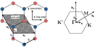
Figure 1: (Color online) Definition of the real space unit-cell (left) and the first Brillouin zone (right). $\mathbf{a_{1}}=(1,0)a$ and $\mathbf{a_{2}}=(-1/2,\sqrt{3}/2)a$ are the lattice vectors in Cartesian coordinates and $|\mathbf{a_{1}}|=|\mathbf{a_{2}}|=a=2.46$ Å is the lattice parameter. $b=1.42$ Å is the inter-atomic distance. The $\mathbf{x}$-axis ($\mathbf{y}$-axis) coressponds to the zig-zag (armchair) direction. $\mathbf{r_{1}}=(1/6,1/3)$ and $\mathbf{r_{2}}=(-1/6,-1/3)$ are the internal coordinates of the carbon atoms in the basis of the lattice vectors. In reciprocal space, $\mathbf{b_{1}}=(1,1/\sqrt{3})2\pi/a$ and $\mathbf{b_{2}}=(0,2/\sqrt{3})2\pi/a$ are the reciprocal lattice vectors in cartesian coordinates. In the Brillouin zone, the high symmetry points $\mathbf{\Gamma}$, $\mathbf{K}$, $\mathbf{K^{\prime}}$ and $\mathbf{M}$ are represented.

In this regime, the electronic structure of doped-graphene is well represented by two Dirac conesCastro Neto et al. (2009) at special points K$=(2/3,0)2\pi/a$ and K${}^{\prime}=(-2/3,0)2\pi/a$ in Cartesian coordinates, see Fig. 1. The x-axis is defined as the zig-zag direction of the graphene sheet, and $a=2.46$ Å is the lattice parameter of graphene. We will extend the validity of the Dirac cones model to $\varepsilon_{F}\lesssim 1.0$ eV by assuming that the so-called trigonal warping of the bands has a negligible effect when the quantities of interest here are angularly averaged. In the absence of electron-phonon scattering the unperturbed Hamiltonian at momentum $\mathbf{k}$ expanded around the Dirac point $\mathbf{K}$ is

$$\mathcal{H}_{\mathbf{K}}(\mathbf{k})=\hbar v_{F}\begin{pmatrix}0&k_{x}-ik_{y}\\ k_{x}+ik_{y}&0\\ \end{pmatrix}$$ (1)

where $v_{F}$ is the Fermi velocity and $\mathbf{k}=(k_{x},k_{y})$ is the electron-momentum measured with respect to the Dirac point $\mathbf{K}$, in a Cartesian basis. It can also be written as $\mathcal{H}_{\mathbf{K}}(\mathbf{k})=\hbar v_{F}\mathbf{k}\cdot\mathbf{\sigma}$, where $\mathbf{\sigma}=(\sigma_{x},\sigma_{y})$ are the Pauli matrices. This Dirac Hamiltonian is written in the pseudospinDas Sarma et al. (2011) basis emerging from the two inequivalent sub-lattices of graphene. It satisfies the eigenvalues equation:

$$\mathcal{H}_{\mathbf{K}}(\mathbf{k})\psi_{\mathbf{k},s}(\mathbf{r})=\varepsilon_{\mathbf{k},s}\psi_{\mathbf{k},s}(\mathbf{r})$$ (2)

with $\varepsilon_{\mathbf{k},s}=s\ \hbar v_{F}|\mathbf{k}|$, and $s=\mp 1$ for the valence $\pi$ and conduction $\pi^{*}$ bands respectively. The Bloch functions are

$$\psi_{\mathbf{k},s}(\mathbf{r})=\frac{1}{\sqrt{N}}e^{i\mathbf{k}\cdot\mathbf{r}}|\mathbf{k},s\rangle$$ (3)

where $N$ is the number of unit-cells in the sample and $|\mathbf{k},s\rangle$ is a pseudospinor eigenfunction, normalized on the unit-cell, corresponding to the in-plane state $\mathbf{k}$ of the band $s$. The eigenfunction $|\mathbf{k},s\rangle$ is defined in the pseudospin basis as:

$$|\mathbf{k},s\rangle=\frac{1}{\sqrt{2S_{\Re}}}\begin{pmatrix}e^{-i\theta_{\mathbf{k}}/2}\\ se^{i\theta_{\mathbf{k}}/2}\end{pmatrix}$$ (4)

where $S_{\Re}=\frac{\sqrt{3}a^{2}}{2}$ is the area of a unit-cell. The angle $\theta_{\mathbf{k}}$ is the angle between $\mathbf{k}$ and the x-axis.

III.2 Phonons

We label $\mathbf{e}_{\mathbf{q},\nu}$ the eigenvector of the dynamical matrix corresponding to the phonon mode $\nu$ of momentum $\mathbf{q}$ and eigenvalue $\omega_{\mathbf{q},\nu}^{2}$. This phonon eigenvector is normalized on the unit-cell and $\omega_{\mathbf{q},\nu}$ is the frequency of the phonon mode. We will discard the coupling to out-of-plane acoustic and optical phonon modes since it is zero by symmetry at the linear orderManes (2007). The components of the vector $\mathbf{e}_{\mathbf{q},\nu}$ are labeled $\mathbf{e}^{a,i}_{\mathbf{q},\nu}$ where $a=1,2$ is an atomic index and $i=1,2$ are the in-plane Cartesian coordinates. We are particularly interested in the small momentum limit of phonons. If we focus on intra-valley scattering, the momentum of phonons that couple to electrons is limited by the extension of the Fermi surface, namely $|\mathbf{q}|\leq 2k_{F}$, where $k_{F}$ is the Fermi wave vector. Near the $\mathbf{\Gamma}=(0,0)$ point (i.e. $|\mathbf{q}|\to 0$), it is customary to use what will be called here the canonical representation of the four in-plane phonon modes to approximate the real ones. The construction of those canonical modes relies on the following rules: i) the eigenvector of a longitudinal (transverse) mode is parallel (perpendicular) to the phonon’s momentum; ii) the phase differences between the two atoms of the unit-cell is $e^{i\mathbf{q}\cdot(\mathbf{r_{1}-r_{2}})}$ for acoustic modes and $-e^{i\mathbf{q}\cdot(\mathbf{r_{1}-r_{2}})}$ for optical modes. This leads to:

$$\mathbf{e}^{a}_{\mathbf{q},\widetilde{\rm{LA}}} = \frac{1}{\sqrt{2}}e^{i\mathbf{q}\cdot(\mathbf{R}+\mathbf{r_{a}})}\frac{\mathbf{q}}{|\mathbf{q}|}$$ (5)

$$\mathbf{e}^{a}_{\mathbf{q},\widetilde{\rm{TA}}} = \frac{1}{\sqrt{2}}e^{i\mathbf{q}\cdot(\mathbf{R}+\mathbf{r_{a}})}\frac{\mathbf{q}_{\perp}}{|\mathbf{q}_{\perp}|}$$

$$\mathbf{e}^{a}_{\mathbf{q},\widetilde{\rm{LO}}} = \gamma_{a}\frac{1}{\sqrt{2}}e^{i\mathbf{q}\cdot(\mathbf{R}+\mathbf{r_{a}})}\frac{\mathbf{q}}{|\mathbf{q}|}$$

$$\mathbf{e}^{a}_{\mathbf{q},\widetilde{\rm{TO}}} = \gamma_{a}\frac{1}{\sqrt{2}}e^{i\mathbf{q}\cdot(\mathbf{R}+\mathbf{r_{a}})}\frac{\mathbf{q}_{\perp}}{|\mathbf{q}_{\perp}|}$$

where $\mathbf{R}$ is the position of the unit-cell, $\mathbf{r_{a}}$ $a=1,2$ are defined in Fig. 1 and $\mathbf{q}_{\perp}$ is such that $\mathbf{q}_{\perp}\cdot\mathbf{q}=0$. $\gamma_{a}=\pm 1$ for $a=1,2$ respectively. The mode indexes $\widetilde{\rm{LA}}$, $\widetilde{\rm{TA}}$ label the canonical longitudinal and transverse acoustic phonon modes, respectively. The canonical longitudinal and transverse optical phonon modes are labeled $\widetilde{\rm{LO}}$ and $\widetilde{\rm{TO}}$ respectively.

As noted in Ref. Manes, 2007, the real phonon modes of graphene at finite momentum tend to the canonical modes in the long wavelength limit. However, at finite momentum, there is some mixing between the canonical acoustic and optical phonon modes in $o(|\mathbf{q}|)$. We find that the use of the canonical eigenvectors leads to a significant error in the following work. Therefore we seek an analytical model for the phonon modes that includes acoustic-optical mixing. We diagonalize the DFT dynamical matrix, calculated by DFT on a small circle around the $\mathbf{\Gamma}$ point. This allows us to obtain the angular dependence in $\mathbf{q}$ at fixed $|\mathbf{q}|$. Comparing the DFT eigenvectors to the canonical ones, we obtain the following expressions:

$$\mathbf{e}_{\mathbf{q},\rm{LA}} = \sqrt{1-\delta^{2}|\mathbf{q}|^{2}}\ \mathbf{e}_{\mathbf{q},\widetilde{\rm{LA}}}-$$

$$\delta\ |\mathbf{q}|\left(\sin(3\theta_{\mathbf{q}})\mathbf{e}_{\mathbf{q},\widetilde{\rm{LO}}}+\cos(3\theta_{\mathbf{q}})\mathbf{e}_{\mathbf{q},\widetilde{\rm{TO}}}\right)$$

$$\mathbf{e}_{\mathbf{q},\rm{TA}} = \sqrt{1-\delta^{2}|\mathbf{q}|^{2}}\ \mathbf{e}_{\mathbf{q},\widetilde{\rm{TA}}}+$$

$$\delta\ |\mathbf{q}|\left(\cos(3\theta_{\mathbf{q}})\mathbf{e}_{\mathbf{q},\widetilde{\rm{LO}}}-\sin(3\theta_{\mathbf{q}})\mathbf{e}_{\mathbf{q},\widetilde{\rm{TO}}}\right)$$

$$\mathbf{e}_{\mathbf{q},\rm{LO}} = \sqrt{1-\delta^{2}|\mathbf{q}|^{2}}\ \mathbf{e}_{\mathbf{q},\widetilde{\rm{LO}}}-$$

$$\delta\ |\mathbf{q}|\left(\sin(3\theta_{\mathbf{q}})\mathbf{e}_{\mathbf{q},\widetilde{\rm{LA}}}+\cos(3\theta_{\mathbf{q}})\mathbf{e}_{\mathbf{q},\widetilde{\rm{TA}}}\right)$$

$$\mathbf{e}_{\mathbf{q},\rm{TO}} = \sqrt{1-\delta^{2}|\mathbf{q}|^{2}}\ \mathbf{e}_{\mathbf{q},\widetilde{\rm{TO}}}+$$

$$\delta\ |\mathbf{q}|\left(\cos(3\theta_{\mathbf{q}})\mathbf{e}_{\mathbf{q},\widetilde{\rm{LA}}}-\sin(3\theta_{\mathbf{q}})\mathbf{e}_{\mathbf{q},\widetilde{\rm{TA}}}\right)$$

Where $\delta\approx 0.10$ Å is a small parameter, and $\theta_{\mathbf{q}}$ is the angle of $\mathbf{q}$ with respect to the x-axis. Our DFT results are consistent with the symmetry-based analysis of Ref. Manes, 2007.

In addition to the intra-valley scattering modes at $\Gamma$, we have to consider the optical A${}_{1}^{\prime}$ inter-valley phonon mode, having momentum $\mathbf{K+q}$, with $\mathbf{q}$ being small. The electron-phonon coupling of these modes will be parametrized as in Ref. Piscanec et al., 2004.
At small $|\mathbf{q}|$, optical phonons frequencies can be considered constant ($\hbar\omega_{\rm{TO}}=\hbar\omega_{\rm{LO}}=0.20$ eV, $\hbar\omega_{\rm{A}_{1}^{\prime}}=0.15$ eV). Acoustic phonon frequencies are of the form $\hbar\omega_{\mathbf{q},\nu}=v_{\nu}|\mathbf{q}|$, where $v_{\nu}$ is the sound velocity of $\nu$ mode (From our DFT calculations, $v_{\rm{TA}}=13.6$ km/s and $v_{\rm{LA}}=21.4$ km/s, independent of the direction).

IV Electron-Phonon matrix elements at finite phonon momentum

In this section we develop the electron-phonon interaction model at small but finite momentum (i.e. $|\mathbf{q}|\to 0$), both analytically and numerically. We use both the canonical and DFT-based eigenvectors of the phonon modes at $\mathbf{\Gamma}$, and compare the results. For the inter-valley scattering A${}_{1}^{\prime}$ mode at $\mathbf{K}$, the model has already been developedPiscanec et al. (2004), and is simply summarized in paragraph IV.3. We will focus on the case of the Hamiltonian expanded around the Dirac point $\mathbf{K}$. Similar results are obtained around $\mathbf{K^{\prime}}$ by complex conjugation and the transformations $\mathbf{k}\to-\mathbf{k}$ and $\mathbf{q}\to-\mathbf{q}$.

In the basis of Dirac pseudospinors, Eq. 4, the small $|\mathbf{q}|$ limit of the derivative of the Dirac Hamiltonian with respect to a general phonon displacement $\mathbf{e}_{\mathbf{q}}$ gives Manes (2007):

$$\Delta\mathcal{H}_{\mathbf{q}}=\Delta\mathcal{H}_{\mathbf{q},\tilde{A}}+\Delta\mathcal{H}_{\mathbf{q},\tilde{O}}$$ (7)

where

$$\Delta\mathcal{H}_{\mathbf{q},\tilde{A}}=i|\mathbf{q}|\times$$ (8)

$$\begin{pmatrix}2\alpha(q)Q_{\widetilde{\rm{LA}}}&\tilde{\beta_{A}}e^{2i\theta_{q}}(Q_{\widetilde{\rm{LA}}}+iQ_{\widetilde{\rm{TA}}})\\ \tilde{\beta_{A}}e^{-2i\theta_{q}}(Q_{\widetilde{\rm{LA}}}-iQ_{\widetilde{\rm{TA}}})&2\alpha(q)Q_{\widetilde{\rm{LA}}}\\ \end{pmatrix}$$

accounts for the canonical in-plane acoustic modes and

$$\Delta\mathcal{H}_{\mathbf{q},\tilde{O}}=i\times$$ (9)

$$\begin{pmatrix}0&\tilde{\beta_{O}}e^{i\theta_{q}}(Q_{\widetilde{\rm{LO}}}+iQ_{\widetilde{\rm{TO}}})\\ \tilde{\beta_{O}}e^{-i\theta_{q}}(Q_{\widetilde{\rm{LO}}}-iQ_{\widetilde{\rm{TO}}})&0\\ \end{pmatrix}$$

accounts for the canonical in-plane optical modes. Parameters $\tilde{\beta_{A}}$ and $\tilde{\beta_{O}}$ are real constants and $\alpha(q)$ is a real function of the norm of the phonon momentum $q=|\mathbf{q}|$. The scalar quantities $Q_{\tilde{\nu}}$ are the components of $\mathbf{e}_{\mathbf{q}}$ in the basis of the canonical eigenvectors, namely:

$$Q_{\tilde{\nu}}=\mathbf{e}_{\mathbf{q}}\cdot\mathbf{e}_{\mathbf{q},\tilde{\nu}}$$ (10)

$\Delta\mathcal{H}_{\mathbf{q},\nu}$ is easily understood as a change of the electronic structure due to the phonon displacement. In more details:

• $\beta$-terms (normally labeled “gauge fields”Pietronero et al. (1980)) in Eqs. 8, 9 are added to the off-diagonal terms of the Dirac Hamiltonian, Eq. 1. They shift the Dirac point in the Brillouin zone without changing its energy. As such, these terms do not alter the overall charge and are unaffected by electronic screening. In a TB model, these terms are related to a variation of the nearest neighbors hopping integral with respect to the in-plane lattice parameter. In a uni-axially strained graphene sheet, the $\beta$-terms correspond to the magnitude of the vector potential (the so-called “synthetic gauge field” von Oppen et al. (2009); Vozmediano et al. (2010); Manes (2007)) that appear in the perturbed terms of the Dirac Hamiltonian. Note that in the presence of a non-uniform strain field, such a synthetic vector potential affects the band structure as an effective magnetic fieldGuinea et al. (2010).

• $\alpha$-term (labeled “deformation potential”) occurs only in the diagonal part of Eq. 8. These terms shift in energy the Dirac point, without changing its position in the Brillouin zone. As they imply a variation of the charge state, they are strongly affected by electronic screening. We use here the screened deformation potential $\alpha(q)$, in contrast with the original model of Ref. Manes, 2007 where screening is ignored and a bare constant deformation potential $\alpha^{bare}$ is used. In a TB model this kind of term corresponds to a variation of the on-site energy. In mechanically strained graphene, it represents the magnitude of the scalar potential or “synthetic electric field” von Oppen et al. (2009); Manes (2007) triggered by a change in the unit cell area.

The EPC matrix elements are defined as

$$g_{\mathbf{k}+\mathbf{q},s,\mathbf{k},s^{\prime},\nu} = \sqrt{\frac{\hbar}{2M\omega_{\mathbf{q},\nu}}}\langle\mathbf{k+q},s|\Delta\mathcal{H}_{\mathbf{q},\nu}|\mathbf{k},s^{\prime}\rangle$$ (11)

where $M$ is the mass of a carbon atom, $|\mathbf{k},s^{\prime}\rangle$ and $|\mathbf{k+q},s\rangle$ are the initial and final electronic states of the scattering process. Since most scattering processes significantly contributing to transport are intra-band, we will drop the $s$ and set $s=s^{\prime}=1$ unless specified otherwise. Setting $s=s^{\prime}=-1$ would give the same final results due to electron-hole symmetry. We further simplify the notation by setting :

$$\langle\mathbf{k+q},1|\Delta\mathcal{H}_{\mathbf{q},\nu}|\mathbf{k},1\rangle=\Delta\mathcal{H}_{\mathbf{q},\nu}(\mathbf{k})$$

We will now study the EPC models obtained using either canonical or DFT phonon modes at $\mathbf{\Gamma}$ with Eq. 7.

IV.1 Coupling to canonical phonon modes at $\mathbf{\Gamma}$

Using the canonical phonon modes, the small phonon-momentum limit ($|\mathbf{q}|\to 0$) of $\Delta\mathcal{H}_{\mathbf{q},\nu}(\mathbf{k})$ can be written as:

$$|\Delta\mathcal{H}_{\mathbf{q},\widetilde{\rm{TA}}}(\mathbf{k})| = \left|\tilde{\beta_{A}}|\mathbf{q}|\sin\left(2\theta_{\mathbf{q}}+\frac{\theta_{\mathbf{k+q}}+\theta_{\mathbf{k}}}{2}\right)\right|$$ (12)

$$|\Delta\mathcal{H}_{\mathbf{q},\widetilde{\rm{LA}}}(\mathbf{k})| = \bigg{|}2\alpha(q)|\mathbf{q}|\cos\left(\frac{\theta_{\mathbf{k+q}}-\theta_{\mathbf{k}}}{2}\right)$$ (13)

$$+ \tilde{\beta_{A}}|\mathbf{q}|\cos\left(2\theta_{\mathbf{q}}+\frac{\theta_{\mathbf{k+q}}+\theta_{\mathbf{k}}}{2}\right)\bigg{|}$$

$$|\Delta\mathcal{H}_{\mathbf{q},\widetilde{\rm{LO}}}(\mathbf{k})| = \left|\tilde{\beta_{O}}\sin\left(\theta_{\mathbf{q}}-\frac{\theta_{\mathbf{k+q}}+\theta_{\mathbf{k}}}{2}\right)\right|$$ (14)

$$|\Delta\mathcal{H}_{\mathbf{q},\widetilde{\rm{TO}}}(\mathbf{k})| = \left|\tilde{\beta_{O}}\cos\left(\theta_{\mathbf{q}}-\frac{\theta_{\mathbf{k+q}}+\theta_{\mathbf{k}}}{2}\right)\right|$$ (15)

These expressions were obtained by symmetry considerations in Ref. Manes, 2007. Using a TB model Venezuela et al. (2011); Piscanec et al. (2004); Pietronero et al. (1980); Park et al. (2014), similar expressions can be obtained. Due to their high energy, $\widetilde{\rm{LO}}$ and $\widetilde{\rm{TO}}$ phonon modes can involve inter-band ($\pi-\pi^{*}$) scattering. However, setting $s=1$ and $s^{\prime}=-1$ simply exchanges the angular dependencies of $\widetilde{\rm{TO}}$ and $\widetilde{\rm{LO}}$. This has no impact in the following transport model since the contributions of those modes are always summed. We can thus keep the above expressions without loss of generality.

IV.2 Coupling to DFT phonon modes at $\mathbf{\Gamma}$

We now insert the DFT phonon modes, Eq. III.2, into the canonical model of Eq. 7. In the expressions for the acoustic DFT eigenvectors (Eq. III.2), the angular dependency and $|\mathbf{q}|$ behavior of the $\widetilde{\rm{TO}}$ and $\widetilde{\rm{LO}}$ components are of the same form as in Eqs. 12 and 13, when considering a circular Fermi surface. It can be shown that the effect of the DFT phonons eigenvectors model on $\Delta\mathcal{H}_{\mathbf{q},\rm{TA}}(\mathbf{k})$ and $\Delta\mathcal{H}_{\mathbf{q},\rm{LA}}(\mathbf{k})$ is then a simple redefinition of the magnitude $\tilde{\beta_{A}}$. Concerning the matrix elements derived from the DFT optical modes, the contribution of the canonical acoustic modes is in $o(|\mathbf{q}|^{2})$ and can be neglected with respect to the dominant $o(1)$ term from the canonical optical modes. Optical EPC matrix elements are thus unaffected by the ab-initio model for phonons.

The small phonon-momentum limit ($|\mathbf{q}|\to 0$) of $\Delta\mathcal{H}_{\mathbf{q},\nu}(\mathbf{k})$ for the DFT modes can then be written :

$$|\Delta\mathcal{H}_{\mathbf{q},\rm{TA}}(\mathbf{k})| = \left|\beta_{A}|\mathbf{q}|\sin\left(2\theta_{\mathbf{q}}+\frac{\theta_{\mathbf{k+q}}+\theta_{\mathbf{k}}}{2}\right)\right|$$ (16)

$$|\Delta\mathcal{H}_{\mathbf{q},\rm{LA}}(\mathbf{k})| = \bigg{|}2\alpha(q)|\mathbf{q}|\cos\left(\frac{\theta_{\mathbf{k+q}}-\theta_{\mathbf{k}}}{2}\right)$$ (17)

$$+ \beta_{A}|\mathbf{q}|\cos\left(2\theta_{\mathbf{q}}+\frac{\theta_{\mathbf{k+q}}+\theta_{\mathbf{k}}}{2}\right)\bigg{|}$$

$$|\Delta\mathcal{H}_{\mathbf{q},\rm{LO}}(\mathbf{k})| = \left|\beta_{O}\sin\left(\frac{\theta_{\mathbf{k+q}}+\theta_{\mathbf{k}}}{2}-\theta_{\mathbf{q}}\right)\right|$$ (18)

$$|\Delta\mathcal{H}_{\mathbf{q},\rm{TO}}(\mathbf{k})| = \left|\beta_{O}\cos\left(\frac{\theta_{\mathbf{k+q}}+\theta_{\mathbf{k}}}{2}-\theta_{\mathbf{q}}\right)\right|$$ (19)

Where $\beta_{A}=\sqrt{1-\delta^{2}|\mathbf{q}|^{2}}\tilde{\beta_{A}}-\delta\tilde{\beta_{O}}\approx\tilde{\beta_{A}}-\delta\tilde{\beta_{O}}$ and $\beta_{O}\approx\tilde{\beta_{O}}$ are effective parameters, and $\alpha(q)$ is unchanged because there are no diagonal terms in Eq. 9.

IV.3 Coupling to inter-valley A${}_{1}^{\prime}$ mode at $\mathbf{K}$

The inter-valley A${}_{1}^{\prime}$ mode at $\mathbf{K}$ scatters an electron from state $\mathbf{k}$ around $\mathbf{K}$ to state $\mathbf{k+q}$ around $\mathbf{K^{\prime}}$, where $\mathbf{q}$ is still small. Using a TB model, it is found to bePiscanec et al. (2004):

$$|\Delta\mathcal{H}_{\mathbf{K+q},\rm{A}_{1}^{\prime}}(\mathbf{k})|=\left|\sqrt{2}\beta_{K}\sin\left(\frac{\theta_{\mathbf{k+q}}-\theta_{\mathbf{k}}}{2}\right)\right|$$ (20)

where $\beta_{K}$ is a real constant. This high energy mode will involve inter-band scattering. In the case $s=-s^{\prime}$, the above expression becomes:

$$|\langle\mathbf{k+q}|\Delta\mathcal{H}_{\mathbf{K+q},\rm{A}_{1}^{\prime}}^{s=-s^{\prime}}|\mathbf{k}\rangle|=\left|\sqrt{2}\beta_{K}\cos\left(\frac{\theta_{\mathbf{k+q}}-\theta_{\mathbf{k}}}{2}\right)\right|$$ (21)

IV.4 Calculation of EPC parameters from DFPT in the linear response.

In this section we perform direct ab-initio calculations of acoustic EPC matrix elements by using density functional perturbation theoryBaroni et al. (2001). The parameters $\beta_{O},\beta_{K}$ for optical phonons have already been evaluated using this methodPiscanec et al. (2004); Venezuela et al. (2011) and compared to experimental Raman measurements. Their numerical values are reported in Table 1. We will mainly focus here on the acoustic phonon EPC parameters.

It is important to underline that this technique do not provide access to the bare deformation potential parameter $\alpha^{bare}$ due to electronic screening. In linear response at small finite (i.e. non-zero) phonon momentum $\mathbf{q}$, the phonon displacement induces a small but finite $\mathbf{q}$-modulated electric field. The electrons screen the finite electric field and consequently the magnitude of EPC. Thus, a finite induced electric field is always present in the linear response calculation at any non-zero phonon momentum and the screened parameter $\alpha(q)$ is obtained.

Concerning the gauge field terms, both the canonical ($\tilde{\beta_{A}}$) and effective ($\beta_{A}$) EPC parameters have been calculated to verify the consistency of our model.

By choosing the phonon momentum ${\bf q}$ along the high symmetry directions $\mathbf{\Gamma}\to\mathbf{K}$ and $\mathbf{\Gamma}\to\mathbf{M}$, we have $\theta_{q}=0$ and $\pi/6$, respectively. If initial and scattered states are taken on a circular iso-energetic line, i.e. if $|\mathbf{k}|=|\mathbf{k+q}|$, then $\frac{\theta_{\mathbf{k+q}}+\theta_{\mathbf{k}}}{2}=\theta_{\mathbf{q}}\pm\frac{\pi}{2}$. From Eqs. 16 and 17 we obtain:

$$|\Delta\mathcal{H}^{(\mathbf{\Gamma\to K})}_{\mathbf{q},\rm{TA}}(\mathbf{k})| = |\mathbf{q}|\beta_{A}$$ (22)

$$|\Delta\mathcal{H}^{(\mathbf{\Gamma\to K})}_{\mathbf{q},\rm{LA}}(\mathbf{k})| = |\mathbf{q}|\left|2\alpha(q)\cos\left(\frac{\theta_{\mathbf{k+q}}-\theta_{\mathbf{q}}}{2}\right)\right|$$ (23)

$$|\Delta\mathcal{H}^{(\mathbf{\Gamma\to M})}_{\mathbf{q},\rm{TA}}(\mathbf{k})| = 0$$ (24)

$$|\Delta\mathcal{H}^{(\mathbf{\Gamma\to M})}_{\mathbf{q},\rm{LA}}(\mathbf{k})| = |\mathbf{q}|\left|\pm\beta_{A}+2\alpha(q)\cos\left(\frac{\theta_{\mathbf{k+q}}-\theta_{\mathbf{q}}}{2}\right)\right|$$

We then consider an iso-energetic line at $\varepsilon=\hbar v_{F}|\mathbf{q}|/2$ and select the electron-momentum ${\bf k}$-point such that $\theta_{\mathbf{k+q}}-\theta_{\mathbf{q}}=\pi$. In this way the cosines in Eqs. 23 and LABEL:eq:DGMLA are null and only the contribution of $\beta_{A}$ coefficient remains. Although we used the notations of the effective model here, the same strategy can be applied to the canonical model. The EPC matrix element is then calculated in either the canonical or DFT eigenvectors basis to obtain $\tilde{\beta_{A}}$ or $\beta_{A}$, respectively. In Fig. 2, we plot the resulting $\tilde{\beta_{A}},\beta_{A}$ for different doping conditions. The fact that the results are the same if evaluated for ${\bf q}$ along $\mathbf{\Gamma}\to\mathbf{K}$ or $\mathbf{\Gamma}\to\mathbf{M}$ confirms the angular dependencies of Eqs. 16 and 17. As expected, the gauge field terms $\tilde{\beta_{A}}$ and $\beta_{A}$ are essentially doping independent and screening has no effect on it. A direct consequence is that scattering by gauge-field is independent of the dielectric background and thus independent of the substrate. The numerical results are reported in the first column of Table 1.

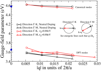
Figure 2: (Color online)Ab-initio calculations of $\frac{|\Delta\mathcal{H}_{\mathbf{q},\rm{LA/TA}}(\mathbf{k})|}{|\mathbf{q}|}$ in high symmetry $(\mathbf{\Gamma}\to\mathbf{M})/(\mathbf{\Gamma}\to\mathbf{K})$ directions respectively lead to gauge field EPC parameters, which depend neither on direction nor doping. $\tilde{\beta_{A}}$($\beta_{A}$) is obtained when the canonical (DFT) phonon modes are used. The blue square and dot at $|\mathbf{q}|=0$ represent the values of $\beta_{A}$ and $\tilde{\beta_{A}}$ found in strained graphene calculations, respectively.

Knowing the value of $\tilde{\beta_{A}}$ and $\beta_{A}$, we adopt a similar strategy to obtain the screened $\alpha(q)$ coefficient by setting $\theta_{\mathbf{k+q}}-\theta_{\mathbf{q}}=2\pi/3$. We find that the $\alpha(q)$ coefficient is smaller than the numeric noise of our simulation. It is then completely negligible with respect to the other parameters.

Table 1: Electron-Phonon Coupling parameters, calculated by different methods: i) DFPT EPC: direct DFPT LDA calculation of EPC, Sec. IV.4. This method does not give access to unscreened $\alpha^{bare}$. ii) $|\mathbf{q}|=0$: from zero-momentum model, see Sec. V. Acoustic parameters are obtained by calculating the magnitude of strained-induced scalar and vector potentials. Optical parameters are obtained with the frozen phonon method from Ref. Lazzeri et al., 2008. iii)TB-DFT: Results obtained in our previous workPark et al. (2014) using a TB model and DFT to calculate the derivative of the hopping parameter with respect to bond-length (see Sec. IV.5). The deformation potential $\alpha^{bare}$ was set to zero in this work. iv) GW calculations of EPC parameters. For phonons at $\mathbf{\Gamma}$, the renormalization is 20$\%$, as the Fermi velocity. For the A${}_{1}^{\prime}$ mode, results are taken from Ref. Attaccalite et al., 2010. v) Exp: Obtained by fitting our numerical solution of Boltzmann transport equation to experiment. $\tilde{\beta_{A}}$ and $\alpha^{bare}$ are not used in the simulations. The values of $\beta_{K}$ in the last line are doping dependent, see Sec. VII for plots (Fig. 5) and discussion.
Note that in a nearest neighbor TB model (third column) $\beta_{K}=\beta_{O}$. This is verifiedPiscanec et al. (2004) within a $1\%$ error in the frameworks of the first two columns. At the GW level however, this equality does not hold.

	DFPT EPC	$|\mathbf{q}|=0$	TB-DFTPark et al. (2014)	GW	Exp
$\tilde{\beta_{A}}$ (eV)	4.60	4.58	3.54	5.52	–
$\beta_{A}$ (eV)	3.60	3.64	3.54	4.32	4.97
$\alpha^{bare}$(eV)	–	2.96	–	–	–
$\beta_{O}=\tilde{\beta_{O}}$ (eV/Å)	9.5	9.5	10.08	11.39	11.39
$\beta_{K}$ (eV/Å)	9.5	9.5	10.08	12.5 $\sim$ 14	17 $\sim$ 40

IV.5 EPC parameters in the tight-binding model

In this section we compare the results of DFPT with other results obtained within the TB model.

In our previous workPark et al. (2014), the canonical phonon modes were used to calculate the perturbation to the TB Hamiltonian. Thus, the canonical EPC parameters $\widetilde{\beta_{A}}$, $\widetilde{\beta_{O}}$ were obtained. In the TB model, $\widetilde{\beta_{A}}$, $\widetilde{\beta_{O}}$ and $\beta_{K}$ are all proportional to the derivative $\eta$ of the nearest neighbor hopping integral with respect to bond-length. Such relationships are obviously very specific to the TB model and are not enforced in the symmetry-based model used here. DFT calculations of $\eta$ resulted in the numerical values of EPC parameters reported in Table 1, column ”TB-DFT”. Those values were also checked against DFPT calculations similar to those presented here. The acoustic EPC obtained in DFPT calculations, using the DFT phonon modes, resulted in what we call here $\beta_{A}$, although the distinction was not made at that time. Indeed, the value of $\widetilde{\beta_{A}}$ in the TB model happens to be close to the values of $\beta_{A}$ found by DFPT. This leads to a very good numerical agreement between the low temperature resistivity calculated in this work and the previous one. However, we would like to point out that this agreement is fortuitous, and in view of the analysis made here, it should be interpreted as a manifestation of the limits of the TB model.

An other way to evaluate EPC matrix elements for acoustic phonons can be found in Refs. Woods and Mahan, 2000; Suzuura and Ando, 2002. The Hamiltonian for electron-phonon is similarly derived from a TB model. The important difference is the use of a microscopic ”valence-force-field”(VFF) model to derive the dynamical matrix and the resulting phonon modes. This model involves two parameters describing the forces resulting from changes in bond-lengths and angles in the lattice. Those parameters are fitted on graphene’s phonon dispersion derived from models using the force-constants measured in graphite. The resulting phonon modes are then inserted in the TB electron-phonon interaction Hamiltonian. Results qualitatively similar to our work are obtained. In particular, a reduction factor originating from the mixing of the acoustic and optical canonical modes appears in the coupling to acoustic modes. The parameter obtained in our DFPT calculations using the canonical phonon modes ($\widetilde{\beta_{A}}$) falls in the interval estimated in Refs. Woods and Mahan, 2000; Suzuura and Ando, 2002. However, the aforementioned reduction factor, equivalent to the ratio $\beta_{A}/\widetilde{\beta_{A}}$, is found to be $\approx 0.5$ in Refs. Woods and Mahan, 2000; Suzuura and Ando, 2002 while we find $\beta_{A}/\widetilde{\beta_{A}}\approx 0.78$.

V Electron-phonon coupling at zone center from finite deformations

In order to calculate the electron-phonon matrix elements in the GW approximation, we calculate the GW band structure for suitably chosen deformation patterns. If the displacement pattern is chosen to reproduce the zero-momentum limit of a given phonon, the matrix elements of the resulting perturbation Hamiltonian can be linked to the EPC parameters. Following this approach, the frozen phonons methodLazzeri et al. (2008) was used to calculate the electron-electron renormalization of the coupling to optical modes (LO, TO, A${}_{1}^{\prime}$) within GW. In order to perform GW calculations and to check the consistency of the small momentum EPC model, we also seek an interpretation of the acoustic EPC parameters at momentum exactly zero. This is achieved by linking acoustic EPC parameters to the perturbation potentials induced by a mechanical strain. This link is then verified numerically at the DFT level. Finally, we present the results of GW calculations for acoustic EPC parameters using this method, and summarize the already existing results on the optical EPC parameters.

V.1 Acoustic EPC and strain-induced potentials

For acoustic phonons at $\Gamma$, a static phonon displacement in the zero momentum limit is equivalent to a strain deformation. We consider the long wavelength limit of an acoustic phonon and the corresponding perturbation occurring on a portion of the graphene sheet of scale $d<<\frac{2\pi}{q}$. Provided there is no long-range (Coulomb) interaction between such zones distant to each other, the phonon perturbation can be seen locally as a simple mechanical strain of the sheet. Author of Ref. Manes, 2007 derived the $|\mathbf{q}|\to 0$ limit of the electron-phonon interaction (Eqs. 12 and 13) for the canonical acoustic modes presented in Sec. IV (Eq. 5). Since screening was ignored in this EPC model, the magnitude of the bare deformation potential $\alpha^{bare}$ was used. In this framework, there is no long-range interaction and strain can be considered to be the exactly $|\mathbf{q}|=0$ equivalent of the $|\mathbf{q}|\to 0$ limit of an acoustic phonon. We will discuss the consequences of screening on the interpretation of the deformation potential in the zero-momentum limit in paragraph V.2.1. We first review the model of strain introduced in Ref. Manes, 2007. This model will be called canonical. The strained unit-cell is defined with the lattice vectors $\mathbf{a^{\prime}_{1}},\mathbf{a^{\prime}_{2}}$ such that :

$$\mathbf{a^{\prime}_{i}} = (\mathcal{I}+\mathcal{U})\ \mathbf{a_{i}}$$ (26)

$$\mathcal{U} = \begin{pmatrix}u_{xx}&u_{xy}\\ u_{yx}&u_{yy}\end{pmatrix}$$ (27)

where $\mathcal{I}$ and $\mathcal{U}$ are the identity matrix and strain tensor, respectively. In this first canonical model, the vectors defining the positions of the carbon atoms in real space are given by the same transformation as the lattice vectors. Namely, the internal coordinates of atoms are unchanged in the basis of the lattice vectors $\{\mathbf{a^{\prime}_{1}},\mathbf{a^{\prime}_{2}}\}$. Evidently, strain also changes the reciprocal lattice vectors according to the transformation $\mathbf{b^{\prime}_{i}}=(\mathcal{I}+\mathcal{U})^{-1}\mathbf{b_{i}}$. It is then natural to develop the Hamiltonian around the special point $\mathbf{K}=(2/3,-1/3)$, as defined in the basis of those new reciprocal lattice vectors. While the coordinates of $\mathbf{K}$ in the basis of the reciprocal lattice vectors are unchanged, it is useful for DFT calculations to note that the Cartesian coordinates of this special point changed compared to the unstrained case. This change is only due to the geometrical redefinition of the lattice vectors. The canonical perturbed Hamiltonian $\mathcal{\widetilde{H}}^{\mathcal{U}}_{\mathbf{K}}$, expanded around point $\mathbf{K}$ of strained graphene is then written in terms of a vector potential $\mathbf{\tilde{A}}=(\tilde{A}_{x},\tilde{A}_{y})$ and a scalar potential $\Phi$Manes (2007):

$$\mathcal{\widetilde{H}}^{\mathcal{U}}_{\mathbf{K}}(\mathbf{k})=\Phi\ \mathcal{I}+(\hbar v_{F}\mathbf{k}+\mathbf{\tilde{A}})\cdot\mathbf{\sigma}$$ (28)

where

$$\tilde{A}_{x} = \sqrt{2}\tilde{\beta_{A}}(u_{xx}-u_{yy})$$ (29)

$$\tilde{A}_{y} = -\sqrt{2}\tilde{\beta_{A}}(u_{xy}+u_{yx})$$ (30)

$$\Phi = \sqrt{2}\alpha^{bare}(u_{xx}+u_{yy})$$ (31)

$\Phi$ acts as a global energy shift while $\mathbf{\tilde{A}}$ yields a redefinition of the Dirac point’s position. In strained graphene and in the presence of gauge fields, it is then important to distinguish special point $\mathbf{K}$ from the Dirac point labeled $\mathbf{\bar{K}}$ here. The former is defined geometrically while the latter is defined as where the $\pi$ and $\pi^{*}$ bands intersect. The Dirac point is now $\mathbf{\bar{K}}=\mathbf{K}-\frac{\mathbf{\tilde{A}}}{\hbar v_{F}}$, as can be seen in Eq. 28. Similar expressions are obtained around the other Dirac cone $\mathbf{K^{\prime}}$, by complex conjugation and the transformations $\mathbf{k}\to-\mathbf{k}$ and $\mathbf{\tilde{A}}\to-\mathbf{\tilde{A}}$.

An addition to the canonical model of EPC Eqs. 12 and 13 was the use of the DFT phonon modes of Eq. III.2. In order to obtain the strain pattern equivalent to the $|\mathbf{q}|=0$ limit of those modes, we allow the relaxation of internal coordinates after imposing a given strain to the crystal axes. This structural optimization of the internal coordinates is crucial as after the strain deformation, there are non-zero forces on the atoms. To give some numerical example, consider the positions of the two carbon atoms as defined in Fig. 1. If we apply to the unit-cell a $1\%$ uni-axial strain in the $\mathbf{y}$-direction,

$$\mathcal{U}=\begin{pmatrix}0&0\\ 0&0.01\end{pmatrix}$$ (32)

and allow the relaxation of internal coordinates, we obtain the new atomic positions $\mathbf{r^{\prime}_{1}}=-\mathbf{r^{\prime}_{2}}\approx 0.9987\times(1/6,1/3)$ in the $\{\mathbf{a^{\prime}_{1}},\mathbf{a^{\prime}_{2}}\}$ basis. As was the case for phonon modes at small momentum, this relaxation has substantial numerical consequences. We assume that the internal coordinates relaxation process leads to a strain model with gauge field parameter $\beta_{A}$ (as in Eqs. 16 and 17) instead of $\tilde{\beta_{A}}$ (as in Eqs. 12 and 13). This is analogous to the effects of using the DFT phonon modes of Eq. III.2 in DFPT. We will thus use the following effective strain model :

$$\mathcal{H}^{\mathcal{U}}_{\mathbf{K}}(\mathbf{k}) = \Phi\ \mathcal{I}+(\hbar v_{F}\mathbf{k}+\mathbf{A})\cdot\mathbf{\sigma}$$ (33)

$$A_{x} = \sqrt{2}\beta_{A}(u_{xx}-u_{yy})$$ (34)

$$A_{y} = -\sqrt{2}\beta_{A}(u_{xy}+u_{yx})$$ (35)

$$\Phi = \sqrt{2}\alpha^{bare}(u_{xx}+u_{yy})$$ (36)

V.2 Calculation of strain-induced potentials at the DFT level

In this section we calculate the changes in the electronic structure of grapheneChoi et al. (2010) under strain within DFT. The magnitudes of the scalar and vector potentials are then extracted from the displacement in the Brillouin zone and the energy shift of the Dirac cone. Within DFT, doping has a negligible effect on this process. By comparing the results to the previous DFPT results, we validate the zero-momentum strain model.

V.2.1 Calculation and interpretation of the strain-induced bare deformation potential

If there are no long-range interactions then the global energy shift $\Phi$ plays the role of the bare deformation potential part of the EPC at $|\mathbf{q}|=0$. Since long-range Coulomb interactions and screening are present in our EPC model, however, an additional complication appears. In finite difference calculations (DFT calculations on strained graphene), differently to what happen in DFPT, the diagonal perturbation $\Phi$ shifts the Dirac Point in energy just by adding a constant potential with no modulation in $\mathbf{q}$. As a result, the scalar potential $\Phi$ obtained with finite differences is bare and does not correspond to the $|\mathbf{q}|\to 0$ limit of the screened deformation potential used in our EPC model. We can obtain the screened $\alpha(q)$ by assuming :

$$\alpha(q)=\frac{\alpha^{bare}}{\epsilon(q)}$$ (37)

where $\epsilon(q)$ is the static dielectric function of graphene in the random-phase approximationAndo (2006); Hwang and Das Sarma (2007).

The parameter $\alpha^{bare}$ is obtained by a global variation of bond-length $b$ and is related to the scalar potential $\Phi$:

$$\mathcal{U} = \begin{pmatrix}\frac{\delta b}{b}&0\\ 0&\frac{\delta b}{b}\end{pmatrix}$$ (38)

$$A_{x} = A_{y}=0$$ (39)

$$\Phi = 2\sqrt{2}\alpha^{bare}\frac{\delta b}{b}$$ (40)

The structure obtained with such biaxial uniform strain is already relaxed. The relaxation process is thus irrelevant for $\alpha^{bare}$, as was the use of canonical or DFT phonon modes for $\alpha(q)$. We obtain the value reported in the second column of Table 1. Using this value and the analytical 2D static dielectric function $\epsilon(q)$, we can evaluate an order of magnitude for $\alpha(q)$ in single layer graphene. In the less screened case of suspended graphene and for $q<2k_{F}$, the dielectric constant is given byAndo (2006); Hwang and Das Sarma (2007):

$$\epsilon(q) = 1+\frac{2\pi e^{2}}{\pi\hbar v_{F}}\frac{2k_{F}}{|\mathbf{q}|}$$ (41)

We find that $\alpha(q)\leq\alpha(q=2k_{F})\approx 0.5$ eV. The presence of a substrate further enhances the screening, reducing this value. Furthermore, as will be seen in Sec. VIII, the relevant quantity to consider for resistivity is the squared ratio of the EPC parameter and sound velocity. The deformation potential term appearing only in the coupling to $\rm{LA}$ phonons while the gauge field term $\beta_{A}$ appears in the coupling to both $\rm{LA}$ and $\rm{TA}$, we have $(\frac{\alpha(q)}{v_{\rm{LA}}})^{2}\approx 5\times 10^{-4}\ll\frac{\beta_{A}^{2}}{v_{\rm{LA}}^{2}+v_{\rm{TA}}^{2}}\approx 0.14$. This is enough to exclude this contribution from the following transport model. In the following, the deformation potential part of EPC will be ignored. In our model, the scattering of electrons by acoustic phonons comes exclusively from the gauge field terms.

V.2.2 Calculation of strain-induced gauge-fields

The parameter $\beta_{A}$ is obtained by applying a strain in the armchair ($\mathbf{y}$) direction:

$$\mathcal{U} = \begin{pmatrix}0&0\\ 0&u_{yy}\end{pmatrix}$$ (42)

$$A_{x} = -\sqrt{2}\beta_{A}u_{yy}$$ (43)

$$A_{y} = \Phi=0$$ (44)

Such uni-axial strain induces a shift in the position of the Dirac point in the $\mathbf{x}$-direction or, equivalently, the opening of a gap $\Delta E_{g}$ at special point $\mathbf{K}$. At this point, the value of the Hamiltonian expanded around $\mathbf{K}$ is :

$$\mathcal{H}^{\mathcal{U}}_{\mathbf{K}}(\mathbf{0})=\begin{pmatrix}0&-\sqrt{2}\beta_{A}u_{yy}\\ -\sqrt{2}\beta_{A}u_{yy}&0\end{pmatrix}$$ (45)

The gap is thus:

$$\Delta E_{g}(\mathbf{0}) = 2\sqrt{2}\beta_{A}u_{yy}$$ (46)

After imposing a strain on the lattice vectors, the internal coordinates of atoms are relaxed within DFT, and the band energies are calculated at special point $\mathbf{K}$. We repeat the process for two values of strain $u_{yy}=-0.01,0.01$. The resulting $\beta_{A}$ is reported in the second column of Table 1.

We repeat the whole process without relaxing the internal coordinates of the atoms and find the value of $\tilde{\beta_{A}}$ reported in Table 1.

The unscreened gauge field parameters $\tilde{\beta_{A}}$ and $\beta_{A}$ are in good agreement with the results of the previous section (see Table 1 and Fig. 2), confirming the validity of the $|\mathbf{q}|\to 0$ and $|\mathbf{q}|=0$ models in our simulation framework. The significant difference between the values of the two parameters emphasizes the necessity of DFT phonons and relaxation. The strain method we propose here for acoustic parameters is especially well-suited for GW calculations since the energy bands are needed only for one $\mathbf{k}$-point.

V.3 EPC parameters at the GW level

Here we discuss how the relevant quantities are renormalized by electron-electron interactions within GW. The Fermi velocity is renormalized by approximately $20\%$, depending slightly on dopingAttaccalite et al. (2010). The renormalization is strongest for neutral (or very low-doped ) graphene ($\approx+21\%$) and slightly decreases with increasing doping ($\approx+17\%$ at $\varepsilon_{F}=1$eV). It can be argued theoreticallyLazzeri et al. (2008); Basko and Aleiner (2008) that the renormalization of the coupling with phonon modes at $\mathbf{\Gamma}$ scales with that of the Fermi velocity because those intra-valley scattering modes involve only a gauge transformation (change in the position of the Dirac cone). This can be illustrated here by noticing that we have for acoustic phonons :

$$|\mathbf{\bar{K}}-\mathbf{K}|=\left|\frac{\mathbf{A}}{\hbar v_{F}}\right|\propto\frac{\beta_{A}}{\hbar v_{F}}$$ (47)

The quantity $|\mathbf{\bar{K}}-\mathbf{K}|$ and the ratio $\frac{\beta_{A}}{\hbar v_{F}}$ are unaffected by electron-electron interactions between low energy Dirac electrons. Indeed, since such interactions are centro-symmetric, their inclusion cannot displace the position of the Dirac cone, both in presence and absence of a strain distortion. Using the frozen phonons method, it was verifiedAttaccalite et al. (2010) that the renormalization of optical modes at $\mathbf{\Gamma}$ is relatively weak and is equal to the renormalization of the Fermi velocity. In order to verify that it is the case for acoustic modes as well, we repeat the process of the previous paragraph within GW. The band energies are calculated at one additional $\mathbf{k}$-point to access the Fermi velocity. We use two different doping levels ($\varepsilon_{F}=0.5$ eV and $0.75$ eV) to study the doping-dependency of the renormalization. The doping levels are rather high to ensure that the Fermi surface is satisfactorily sampled by our grid. The results are presented in Table 2.

Table 2: Renormalization of Fermi velocity and acoustic gauge field parameter by electron-electron interactions within GW, presented for two different values of doping and for uniaxial strain $u_{yy}=-0.01,+0.01$ as explained in Sec. V.2.

Strain $u_{yy}$	$-0.01$		$+0.01$
Fermi energy $\varepsilon_{F}$	$0.50$ eV	$0.75$ eV	$0.50$ eV	$0.75$ eV
$v_{F}^{GW}/v_{F}^{DFT}$	$1.203$	$1.166$	$1.204$	$1.164$
$\beta_{A}^{GW}/\beta_{A}^{DFT}$	$1.215$	$1.172$	$1.202$	$1.165$

Our calculations confirm the $\approx 20\%$ renormalization of $v_{F}$ at low doping. More importantly, they confirm what was assumed in our previous workPark et al. (2014), namely that the electron-electron interactions renormalize $\beta_{A}$ as the Fermi velocity:

$$\frac{v_{F}^{GW}}{v_{F}^{DFT}}\approx\frac{\beta_{A}^{GW}}{\beta_{A}^{DFT}}$$

In contrast, the interaction of electrons with inter-valley A${}_{1}^{\prime}$ mode is not just a gauge transformation of the electronic Hamiltonian. The renormalization of this mode is much stronger overall, and its doping dependency is more pronounced. According to Ref. Attaccalite et al., 2010, $\beta_{K}$ is renormalized by $\approx+46\%$ close to neutrality, and $\approx 20\%$ at $\varepsilon_{F}=1$eV.

As will be discussed in more details in the rest of this paper, the contribution to the resistivity of each phonon modes is proportional to the squared ratio of the EPC parameter and the Fermi velocity. For the phonon modes at $\mathbf{\Gamma}$, the Fermi velocity renormalization is exactly compensated by the electron-phonon coupling renormalization. The GW corrections thus has no effect on their contribution resistivity. The A${}_{1}^{\prime}$ mode, on the other hand, is renormalized more strongly than the Fermi velocity. Therefore, we have to choose relevant values of the renormalization for both the Fermi velocity and $\beta_{K}$. In Sec. VII, we will see that the available experimental data allows for a comparison of the value of $\beta_{K}$ only in a short range of doping close to neutrality ($0.12\to 0.21$eV).

In view of the above remarks, we use in our resistivity simulations the $+46\%$ renormalization of $\beta_{K}$ obtained at neutrality by Ref. Attaccalite et al., 2010. We then choose the corresponding $+20\%$ renormalization of the Fermi velocity, relevant at low doping. Finally, the coupling to phonons modes at $\mathbf{\Gamma}$ ($\beta_{A}$, $\beta_{O}$) are renormalized by $+20\%$, as the Fermi velocity.

VI Boltzmann transport theory

In this section we present a numerical solution to the Boltzmann transport equation for phonon-limited transport in graphene. The general method presented here is well known in carrier transport theory and has been applied to some extent to grapheneSuzuura and Ando (2002); Shishir and Ferry (2009); Perebeinos and Avouris (2010); Mariani and von Oppen (2010); Hwang and DasSarma (2008); Hwang et al. (2007). The central addition to those previous works resides in the treatment of a more complete EPC model, and a numerical solution involving very few approximations. The initial steps are repeated in an effort to clarify the assumptions involved.

A carrier current is created by applying an electric field $\mathbf{E}$. This has the effect of changing the electronic distribution $f(\mathbf{k})$. In the steady state regime, the new distribution favors states with electron momentum $\mathbf{k}$ in the opposite direction of the electric field, thus creating a net current $\mathbf{j}$. We are interested in the current in the direction of the electric field that we choose to be the $\mathbf{x}$-axis, used as a reference for angles in our model. Throughout this work, the resistivity is to be understood as the diagonal part of the resistivity tensor $\rho=\rho_{xx}$. It is given byAshcroft and Mermin (1976):

$$\frac{1}{\rho}=\frac{\mathbf{j}\cdot\mathbf{x}}{|\mathbf{E}|}=\frac{2e}{|\mathbf{E}|}\int_{BZ}\frac{d\mathbf{k}}{(2\pi)^{2}}f(\mathbf{k})\mathbf{v(k)}\cdot\mathbf{x}$$ (48)

The integral is made over the Brillouin zone with a factor $2$ for spin degeneracy, $e$ is the elementary charge, $\mathbf{v(k)}$ is the carrier velocity of state $|\mathbf{k}\rangle$, and $\mathbf{x}$ is the Cartesian coordinate basis vector. In the framework of linear response theory, we are interested in the response of $f(\mathbf{k})$ to the first order in electric fieldNag (1980); Kawamura and Das Sarma (1992); Basu and Nag (1980). Consistent with the Dirac cone model, we assume $\varepsilon_{\mathbf{k}}=\hbar v_{F}|\mathbf{k}|$ and $\mathbf{v(k)}=v_{F}\frac{\mathbf{k}}{|\mathbf{k}|}$. We then separate the norm and angular dependency of $\mathbf{k}$ in $f(\mathbf{k})=f(\varepsilon_{\mathbf{k}},\theta_{\mathbf{k}})$ and consider the first order expansion:

$$f(\varepsilon_{\mathbf{k}},\theta_{\mathbf{k}})=f^{(0)}(\varepsilon_{\mathbf{k}})+f^{(1)}(\varepsilon_{\mathbf{k}},\theta_{\mathbf{k}})$$ (49)

where $f^{(1)}$ is proportional to the electric field, and $f^{(0)}$ is the equilibrium Fermi-Dirac distribution, which has no angular dependency. Due to graphene symmetries, the two Dirac cones of the Brillouin zone give the same contribution to Eq. 48. Multiplying by a factor 2 for valley degeneracy, performing the dot product, and using $f$, Eq. 48 becomes:

$$\frac{1}{\rho}=\frac{4e}{|\mathbf{E}|}\int_{\mathbf{K}}\frac{d\mathbf{k}}{(2\pi)^{2}}f^{(1)}(\varepsilon_{\mathbf{k}},\theta_{\mathbf{k}})v_{F}\cos(\theta_{\mathbf{k}})$$ (50)

where the integral is now carried out within a circular region around $\mathbf{K}$. It is clear that the zeroth order term gives no contribution due to the angular integral, and that we have to look for $f^{(1)}\propto\cos(\theta_{\mathbf{k}})$.

We now use Boltzmann transport equation to obtain the energy dependency of $f^{(1)}$. A key quantity is the collision integral $\left(\frac{\partial f}{\partial t}\right)_{coll}(\mathbf{k})$ describing the rate of change in the occupation of the electronic state $|\mathbf{k}\rangle$ due to scattering. Assuming that the electronic distribution is in a spatially uniform, out-of-equilibrium but steady state, the change of the occupation function triggered by the electric field must be compensated by the change due to collisionsAshcroft and Mermin (1976):

$$-\frac{e\mathbf{E}}{\hbar}\cdot\frac{\partial f}{\partial\mathbf{k}}=\left(\frac{\partial f}{\partial t}\right)_{coll}(\mathbf{k})\\$$ (51)

Using Fermi golden rule, the collision integral is:

$$\left(\frac{\partial f}{\partial t}\right)_{coll}(\mathbf{k})=$$ (52)

$$\sum_{\mathbf{k^{\prime}}}\left\{P_{\mathbf{k^{\prime}}\mathbf{k}}f(\mathbf{k^{\prime}})(1-f(\mathbf{k}))-P_{\mathbf{k}\mathbf{k^{\prime}}}f(\mathbf{k})(1-f(\mathbf{k^{\prime}}))\right\}$$

Here, $\mathbf{k}$ belongs to a circular region around $\mathbf{K}$. The momentum of the scattered states $\mathbf{k^{\prime}}$ is i) around $\mathbf{K}$ for intra-valley scattering modes; ii) around the other Dirac cone $\mathbf{K^{\prime}}$ in case of inter-valley scattering. The quantity $P_{\mathbf{k}\mathbf{k^{\prime}}}$ is the scattering probability from state $|\mathbf{k}\rangle$ to $|\mathbf{k^{\prime}}\rangle$. It satisfies the detailed balance condition, namely:

$$P_{\mathbf{k^{\prime}}\mathbf{k}}f^{(0)}(\varepsilon_{\mathbf{k^{\prime}}})(1-f^{(0)}(\varepsilon_{\mathbf{k}}))=P_{\mathbf{k}\mathbf{k^{\prime}}}f^{(0)}(\varepsilon_{\mathbf{k}})(1-f^{(0)}(\varepsilon_{\mathbf{k^{\prime}}}))$$

(53)

The scattering probability $P_{\mathbf{k}\mathbf{k^{\prime}}}$ is composed of two terms,

$$P_{\mathbf{k}\mathbf{k^{\prime}}}=P_{\mathbf{k}\mathbf{k^{\prime}},\rm{I}}+\sum_{\nu}P_{\mathbf{k}\mathbf{k^{\prime}},\nu}$$ (54)

where $P_{\mathbf{k}\mathbf{k^{\prime}},\rm{I}}$ is the impurity scattering probability and $P_{\mathbf{k}\mathbf{k^{\prime}},\nu}$ is due to the electron-phonon scattering of the $\nu^{\rm th}$ phonon branch.

In the Born approximation, the impurity scattering probability is

$$P_{\mathbf{k}\mathbf{k^{\prime}},\rm{I}} = \frac{2\pi}{\hbar}\frac{1}{N}n_{i}|\langle\mathbf{k}|H_{i}|\mathbf{k^{\prime}}\rangle|^{2}\delta(\varepsilon_{\mathbf{k}}-\varepsilon_{\mathbf{k^{\prime}}})$$ (55)

where $H_{i}$ is the electron-impurity interaction Hamiltonian, $n_{i}$ the impurity density and $N$ is the number of unit cells. When needed for comparison with experiment, we use existing methodsHwang et al. (2007); Hwang and Das Sarma (2008); Barreiro et al. (2009) to fit charged and short-range impurity densities on the low temperature resistivity measurements. The electron-phonon scattering probability is given by

$$P_{\mathbf{k},\mathbf{k+q},\nu} = \frac{2\pi}{\hbar}\frac{1}{N}|g_{\mathbf{k+q},\mathbf{k},\nu}|^{2}\left\{n_{q,\nu}\delta(\varepsilon_{\mathbf{k+q}}-\varepsilon_{\mathbf{k}}-\hbar\omega_{\mathbf{q},\nu})\right.$$ (56)

$$+ \left.(n_{q,\nu}+1)\delta(\varepsilon_{\mathbf{k+q}}-\varepsilon_{\mathbf{k}}+\hbar\omega_{\mathbf{q},\nu})\right\}$$

where $\mathbf{k+q}=\mathbf{k^{\prime}}$, $g_{\mathbf{k+q},\mathbf{k},\nu}$ is the electron-phonon matrix element introduced in Eq. 11 and $n_{q,\nu}$ is the Bose-Einstein equilibrium occupation of mode $\nu$ with phonon-momentum ${\bf q}$ and phonon frequency $\omega_{\mathbf{q},\nu}$.

By Replacing Eq. 49 in Eq. 52, using Eq. 53 and keeping only first order terms we obtain

$$-\frac{e\mathbf{E}}{\hbar}\cdot\frac{\partial f}{\partial\mathbf{k}}=\sum_{\mathbf{k^{\prime}}}P_{\mathbf{k}\mathbf{k^{\prime}}}\frac{1-f^{(0)}(\varepsilon_{\mathbf{k^{\prime}}})}{1-f^{(0)}(\varepsilon_{\mathbf{k}})}\Big{(}f^{(1)}(\varepsilon_{\mathbf{k^{\prime}}},\theta_{\mathbf{k^{\prime}}})\frac{f^{(0)}(\varepsilon_{\mathbf{k}})(1-f^{(0)}(\varepsilon_{\mathbf{k}}))}{f^{(0)}(\varepsilon_{\mathbf{k^{\prime}}})(1-f^{(0)}(\varepsilon_{\mathbf{k^{\prime}}}))}-f^{(1)}(\varepsilon_{\mathbf{k}},\theta_{\mathbf{k}})\Big{)}$$ (57)

We first consider the left-hand side of Eq. 57 and, looking for a solution that is first order in the electric field, we have:

$$-\frac{e\mathbf{E}}{\hbar}\cdot\frac{\partial f}{\partial\mathbf{k}} = -F\cos(\theta_{\mathbf{k}})\hbar v_{F}\frac{\partial f^{(0)}}{\partial\varepsilon}(\varepsilon_{\mathbf{k}})$$ (58)

with $F=\frac{e|\mathbf{E}|}{\hbar}$. In the right-hand-side of Eq. 57 we adoptKawamura and Das Sarma (1992) the following ansatz for $f^{(1)}(\varepsilon_{\mathbf{k}},\theta_{\mathbf{k}})$:

$$f^{(1)}(\varepsilon_{\mathbf{k}},\theta_{\mathbf{k}})=F\tau(\varepsilon_{\mathbf{k}})\cos(\theta_{\mathbf{k}})\hbar v_{F}\frac{\partial f^{(0)}}{\partial\varepsilon}(\varepsilon_{\mathbf{k}})$$ (59)

and verify that it solves Eq. 57. The energy dependency of $f^{(1)}$ is captured by $\tau(\varepsilon_{\mathbf{k}})$. This auxiliary variable has the dimension of time. The time $\tau(\varepsilon_{\mathbf{k}})$ depends on the perturbation and has a meaning only in the the framework studied here, namely the steady state of a distribution under an external electric field. It is different from the relaxation time from relaxation time approximation and from the scattering time as can be measured by angle resolved photoemission spectroscopy.

By replacing Eqs. 58 , 59 in Eq. 57 we obtain the following equation, as in Refs. Nag, 1980; Kawamura and Das Sarma, 1992; Basu and Nag, 1980, and dividing both members by $\cos(\theta_{\mathbf{k}})$ we obtain:

$$1 = \sum_{\mathbf{k^{\prime}}}P_{\mathbf{k}\mathbf{k^{\prime}}}\frac{1-f^{(0)}(\varepsilon_{\mathbf{k^{\prime}}})}{1-f^{(0)}(\varepsilon_{\mathbf{k}})}\left(\tau(\varepsilon_{\mathbf{k}})-\tau(\varepsilon_{\mathbf{k^{\prime}}})\frac{\cos(\theta_{\mathbf{k^{\prime}}})}{\cos(\theta_{\mathbf{k}})}\right)$$

We then parametrize $\mathbf{k}$-space in energy (equivalent to norm through $\varepsilon=\hbar v_{F}|\mathbf{k}|$). On an energy grid of step $\Delta\varepsilon$, Eq. LABEL:eq:BT1 can be written:

$$\sum_{\varepsilon^{\prime}}\mathcal{M}_{\varepsilon,\varepsilon^{\prime}}\tau(\varepsilon^{\prime})=1$$

where $\varepsilon=\hbar v_{F}|\mathbf{k}|$, $\varepsilon^{\prime}=\hbar v_{F}|\mathbf{k^{\prime}}|$ and the matrix $\mathcal{M}$ is defined in appendix A. The time $\tau$ can then be obtained by numerical inversion of the matrix $\mathcal{M}$ (see App. A for more details).

It is worthwhile to recall that, due to the additivity of the scattering probabilities in Eq. 54, the matrix $\mathcal{M}$ involves a sum over impurities and different phonon bands, namely $\mathcal{M}=\mathcal{M}_{\rm{I}}+\sum_{\nu}\mathcal{M}_{\nu}$. Strictly speaking, the time $\tau$ is obtained from the inversion of the global matrix $\mathcal{M}$ and not from the sum of the inverse of the matrices $\mathcal{M}_{\nu}$ and $\mathcal{M}_{\rm{I}}$. The latter is equivalent to applying Matthiessen’s rule, which is an approximation (see Sec. VIII).

From the time $\tau$ we obtain the distribution function. Inserting it into Eq. 48, the electrical resistivity is found by evaluating the following integral numerically:

$$\frac{1}{\rho} =\frac{e^{2}v_{F}^{2}}{2}\int d\varepsilon DOS(\varepsilon)\tau(\varepsilon)\left(-\frac{\partial f^{(0)}}{\partial\varepsilon}(\varepsilon)\right)$$ (61)

Where $DOS(\varepsilon_{\mathbf{k}})=\frac{2|\varepsilon_{\mathbf{k}}|}{\pi(\hbar v_{F})^{2}}$ is the total density of states per unit area of graphene, valley and spin degeneracy included.

VII Results

Experiment	I	II
Temp. range (K)	$4\sim 250$	$14\sim 480$
Doping range (eV)	$0.36\sim 1.01$	$0.09\sim 0.21$
Gate dielectric	PEO	SiO2

Table 3: Sources of the experimental data used in this section. Experiment I and II correspond to Ref. Efetov and Kim, 2010 and Ref. Chen et al., 2008 respectively. Combining those two experiments provides us with a wide range of temperature and doping conditions. PEO stands for poly(ethylene)oxide.

Table 4: Numerical values of parameters used in resistivity calculations. The effective sound velocity $v_{\rm{A}}$ is defined in Eq. 66.

Parameter	symbol	Value
Acoustic gauge field (GW)	$\beta_{A}$	$4.32$ eV
Acoustic gauge field (fitted)	$\beta_{A}$	$4.97$ eV
Optical gauge field (GW)	$\beta_{O}$	$11.4$ eV/Å
A${}_{1}^{\prime}$ EPC parameter (GW)	$\beta_{K}$	$13.9$ eV/Å
A${}_{1}^{\prime}$ EPC parameter (fitted)	$\beta_{K}$	see Fig. 5
Lattice parameter	$a$	$2.46$ Å
Unit-cell area	$S_{\Re}$	$5.24$ Å2
Sound velocity TA	$v_{\rm{TA}}$	$13.6$ km.s-1
Sound velocity LA	$v_{\rm{LA}}$	$21.4$ km.s-1
Effective sound velocity	$v_{\rm{A}}$	$16.23$ km.s-1
LO/TO phonon energy	$\hbar\omega_{\rm{LO}/\rm{TO}}$	$0.20$ eV
A${}_{1}^{\prime}$ phonon energy	$\hbar\omega_{\rm{A}_{1}^{\prime}}$	$0.15$ eV
Carbon atom mass	$M$	$12.0107$ u
Mass density	$\mu_{S}=2M/S_{\Re}$	$7.66$ kg/m2
Fermi Velocity (GW)	$v_{F}$	$1.00$ $10^{6}$ ms-1

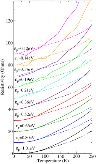
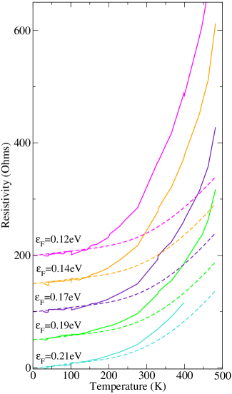
Figure 3: (Color online) Comparison of experimental data (plain lines) and the numerical solution of the Boltzmann equation (dashed lines) in the Bloch-Grüneisen and Equipartition regimes(a) and in the HT regime(b), for several doping levels ranging from $\varepsilon_{F}=0.12$ eV to $\varepsilon_{F}=1.01$ eV. Experimental data are from Refs. Chen et al., 2008 ($0.12\to 0.21$eV) and Efetov and Kim, 2010 ($0.36\to 1.01$eV). For each curve, the residual resistivity was subtracted, then a fictitious residual resistivity was added for clarity of the plot (different values were used in the two plots). Though their value has no absolute sense, the fictitious resistivities are ordered as the real ones.

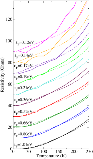
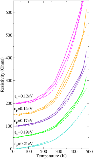
Figure 4: (Color online) Results presented as in Fig. 3, with fitted values for $\beta_{A}$ (see Table 1) and $\beta_{K}$ (see Fig. 5) in the simulations. Experimental data from a different sample are added in plain lines in Fig. 4 to show that the sample-to-sample discrepancy when approaching the Dirac point is of the same order as the disagreement with the fitted numerical model.

On general grounds, three different regimes are present in our calculations. These three regimes depend on three energy scales: i) the Fermi energy $\varepsilon_{F}$ is the reference energy around which initial and scattered states are situated; ii) the phonon energy $\hbar\omega$ is the energy difference between initial and scattered states; iii) the temperature $k_{B}T$ sets the interval on which electronic and phonon occupations vary. Comparing $\hbar\omega$ to $\varepsilon_{F}$ indicates how much the density of states changes during a scattering process. Comparing $\hbar\omega$ to $k_{B}T$ indicates phonon occupations and the change of electronic occupations. Based on those observations, we have:

• Bloch-Grüneisen (BG) regime ($0K<T\lesssim 0.15\times T_{BG}$ where $T_{BG}=2\hbar v_{TA/LA}k_{F}/k_{B}$). At these temperatures, $k_{B}T$ is small compared to the energy of optical phonons. Those modes are not occupied and do not contribute. In contrast, the acoustic modes contribute since $k_{B}T$ is of the order of $\hbar\omega_{\mathbf{q},\rm{TA}/\rm{LA}}$. Moreover, the occupancy of initial states $f(\varepsilon_{\mathbf{k}})$ and scattered states $f(\varepsilon_{\mathbf{k}}\pm\hbar\omega_{\mathbf{q},\rm{TA}/\rm{LA}})$ are significantly different. Finally, as $\hbar\omega_{\mathbf{q},\rm{TA}/\rm{LA}}<<\varepsilon_{F}$, quantities other than occupancy, such as the density of states, can be considered constant. In this regime, the resistivity has a $\propto T^{4}$ dependence due to acoustic phonons.

• Equipartition (EP) regime ($0.15\times T_{BG}\lesssim T\lesssim 0.15\times\hbar\omega_{A_{1}^{\prime}}\approx 270$K): optical phonons still do not contribute. As $\hbar\omega_{\mathbf{q},\rm{TA}/\rm{LA}}<<k_{B}T<<\varepsilon_{F}$ the scattering by acoustic phonons can be approximated as elastic, including in the occupancies of initial and final states. The resulting resistivity is then linear in temperature.

• High temperature (HT) regime ($T\gtrsim 0.15\times\hbar\omega_{A_{1}^{\prime}}\approx 270$K) : the elastic approximation for acoustic phonons holds, but the three energy scales are comparable in the case of optical phonons. In this case, no reasonable approximation can be made globally. The optical phonon participation is characterized by a strongly increasing resistivity at a temperature around $15\%$ of the phonon energy. Due to their lower energy and stronger coupling, the contribution of optical A${}_{1}^{\prime}$ phonons is more pronounced than LO/TO phonons.

Our calculated resistivity is compared with experimental data in Fig. 3. Experimental data are from the references cited in Table 3 and the computational parameters are summarized in Table 4.

Below room temperature, Fig. 3, the comparison between theory and experiment is meaningful only above $\varepsilon_{F}\gtrsim 0.14$eV. Indeed, when approaching the Dirac pointDas Sarma and Hwang (2013), the electron density tends to zero and resistivity diverges. One has to adopt a model with non-homogenous electron densityMartin et al. (2007) to obtain a finite resistivity, such that the Fermi energy is ill-defined. Temperature-dependent screening of impurity scattering as well as temperature-dependent chemical potential shiftHwang and Das Sarma (2009) also play a role in this regime. Those issues are not treated in our model. At sufficiently high doping, the temperature behavior of BG and EP regimes are well reproduced, despite an overall underestimation. The doping-dependency of the resistivity is limited to the BG ($\rho\propto T^{4}$) regime. The upper boundary of this regime increases with doping, since $T_{BG}\propto k_{F}$. Above $\sim 0.15\times T_{BG}$, in the EP regime, the slope of the resistivity is essentially doping independent. This confirms that the deformation potential term can be neglected, since its screening would induce such a dependency.

In the HT regime, Fig. 3, the underestimation is globally more pronounced. The increase of experimental resistivity around room temperature is steeper than the theoretical one. A strong doping dependency of the experimental curves appear. The agreement with the simulations improves as the system is doped far away from the Dirac point. Usually this discrepancy is attributed to remote-phonon scattering from the SiO₂ substrateChen et al. (2008). This effect is missing in our calculation as the substrate is not included. Moreover, we found no experimental data on other substrates for those temperatures. It follows that substrate dependent sources of scattering cannot be ruled out in the HT regime. However, we would like to point out that based on the observation that the contribution of optical phonons seems to appear at a temperature $\approx 0.15\times\hbar\omega_{\nu}$, we expect intrinsic optical phonons to be better candidates than the relatively low energy remote-phonons proposed in Ref. Chen et al., 2008. The optical A${}_{1}^{\prime}$ mode at $\mathbf{K}$ does induce a sudden increase of resistivity, and the temperature at which this occurs is in very good agreement with experiment. The increasing discrepancy between theory and experiment in the magnitude of resistivity at lower doping could be explained by the fact that the EPC parameter $\beta_{K}$ corresponding to the A${}_{1}^{\prime}$ mode is renormalized by electron-electron interactionAttaccalite et al. (2010). This renormalization decreases the larger the electron-doping of graphene, and tends to the DFT value at high doping.

We then fit the value of $\beta_{A}$ for acoustic modes on experimental data in the EP regime. We find that an increase of the electron-phonon coupling of the acoustic modes of $15\%$ leads to an excellent agreement with experimental data in the BG and EP regimes, as shown in Fig. 4. We found an equivalent agreement for resistivity measurements of graphene on h-BNDean et al. (2010) or on SiO₂ with HfO₂ gate dielectricZou et al. (2010), thus ruling out any significant contribution from substrate dependent sources of scattering (other than charged and short-range impurities) in the BG and EP regimes. We then conclude that the solution of the Boltzmann equation based on DFT and GW (the two methods are equivalent here) electron-phonon coupling parameters and bands explains fairly well the low-temperature regime (BG and EP), although DFT seems to underestimate the coupling to acoustic modes by $15\%$, or the resistivity by $\approx 30\%$. On closer inspection (see Sec. VIII and App. B), the resistivity in the EP regime is proportional to $\frac{\beta^{2}_{A}}{v_{\rm{A}}^{2}}$ where $v_{\rm{A}}$ is the effective sound velocity given in Table 4. An overestimation of $v_{\rm{A}}$ could also explain the $30\%$ underestimation of the resistivity. Finally, this discrepancy might be partly due to some other $\propto T$ contribution from processes ignored here, such as impurity scattering with temperature-dependent screeningHwang and Das Sarma (2009). In any case, defining an effective parameter $\beta_{A}$ with the fitted value found here is sufficient to describe low temperature resistivity in a relatively large range of doping levels.

Within such a picture, we fit the optical $\beta_{K}$ parameter as a function of doping. The fitted values of $\beta_{K}$ are plotted in Fig. 5, along with GW and DFT values. Near the Dirac point, the fitted coupling parameter increases substantially more than previous estimatesAttaccalite et al. (2010) at the GW level, but at high doping it seems to approach the DFT value. We then plot the resistivity with the fitted $\beta_{A}$ and $\beta_{K}$, and find a good agreement with experiments on Fig. 4. However, since the screened coupling to remote phonon has a similar behavior as a function of doping, it is not possible to rule out this effect.

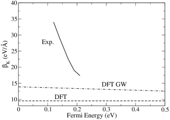
Figure 5: The parameter $\beta_{K}$ fitted on experimental results as a function of Fermi energy is compared to the DFT LDA and DFT GW values. The DFT GW values are from Ref. Attaccalite et al., 2010.

VIII Approximated solutions

In this section we seek a compromise between analytical simplicity and numerical accuracy. We review some of the approximations often made in transport models, and check their validity against the full numerical solution presented in Sec. VI. Fitted EPC parameters are used in the resistivity calculations.

VIII.1 Semi-analytical approximated solution

The first essential step is to derive an analytical expression of the time $\tau_{\nu}(\varepsilon_{\mathbf{k}})$ for each phonon branch. We first rewrite equation LABEL:eq:BT1 as:

$$\frac{1}{\tau(\varepsilon_{\mathbf{k}})} = \sum_{\mathbf{k^{\prime}}}P_{\mathbf{k}\mathbf{k^{\prime}}}\frac{1-f^{(0)}(\varepsilon_{\mathbf{k^{\prime}}})}{1-f^{(0)}(\varepsilon_{\mathbf{k}})}$$ (62)

$$\times\Big{(}1-\frac{\tau(\varepsilon_{\mathbf{k^{\prime}}})\cos(\theta_{\mathbf{k^{\prime}}})}{\tau(\varepsilon_{\mathbf{k}})\cos(\theta_{\mathbf{k}})}\Big{)}$$

For the doping level considered here, impurity scattering is essentially constant on the energy scale of the phonon energies. When this type of scattering dominates, the approximation $\tau(\varepsilon_{\mathbf{k^{\prime}}})\approx\tau(\varepsilon_{\mathbf{k}})$ becomes reasonable. We can simplify $\tau(\varepsilon_{\mathbf{k}})$ on the right-hand side of Eq. 62 and write:

$$\frac{1}{\tau(\varepsilon_{\mathbf{k}})}=\sum_{\nu}\frac{1}{\tau_{\nu}(\varepsilon_{\mathbf{k}})}$$ (63)

In other words, Matthiessen’s ruleMatthiessen and Vogt (1864) can be applied. With mild restrictions on the form of the angular dependency of the scattering probability, one can then use the following expression for the times $\tau_{\nu}$Kaasbjerg et al. (2012); Hwang and DasSarma (2008):

$$\frac{1}{\tau_{\nu}(\varepsilon_{\mathbf{k}})}\approx\sum_{\mathbf{k^{\prime}}}P_{\mathbf{k}\mathbf{k^{\prime}},\nu}\frac{1-f^{(0)}(\varepsilon_{\mathbf{k^{\prime}}})}{1-f^{(0)}(\varepsilon_{\mathbf{k}})}\Big{(}1-\cos(\theta_{\mathbf{k^{\prime}}}-\theta_{\mathbf{k}})\Big{)}\\$$ (64)

A solution of Eq. 64 can now be carried out for different times separately by using phonon-specific approximations. Details can be found in App. B. We present here a solution that is relatively simple, yet very close to the complete one in a large range of temperature. For the sum of TA and LA acoustic phonons, labeled by the index $\rm{A}\equiv\rm{TA}+\rm{LA}$, we use the time derived in the EP and HT regime:

$$\left(\frac{1}{\tau_{\rm{A}}(\varepsilon_{\mathbf{k}})}\right)_{\rm{EP,HT}}=\frac{2\beta_{A}^{2}k_{B}T}{\mu_{S}\hbar v_{\rm{A}}^{2}}\frac{\varepsilon_{\mathbf{k}}}{(\hbar v_{F})^{2}}\\$$ (65)

where $\mu_{S}=2M/S_{\Re}$ is the mass density per unit area of graphene. The full derivation can be found in App. C. The effective sound velocity for the sum of TA and LA contributions $v_{\rm{A}}$ is such that:

$$\frac{2}{v_{\rm{A}}^{2}}=\frac{1}{v_{\rm{TA}}^{2}}+\frac{1}{v_{\rm{LA}}^{2}}$$ (66)

For the sum of LO and TO phonons, labeled by $\rm{O}\equiv\rm{LO}+\rm{TO}$, we use no other approximation than the constant phonon dispersion ($\hbar\omega_{\rm{LO}}=\hbar\omega_{\rm{TO}}=\hbar\omega_{\rm{O}}=0.20$ eV) and find the expression given in Eq. 76 of App. B. The same approximation is made for Optical A${}_{1}^{\prime}$ phonons at K ($\hbar\omega_{\rm{A}_{1}^{\prime}}=0.15$ eV) and we find the expression given in Eq. B.4 of App. B. Finally, impurity scattering can be easily included knowing the residual resistivity $\rho_{\rm{I}}(T=0)=\rho(T=0)$:

$$\frac{1}{\tau_{\rm{I}}(\varepsilon_{\mathbf{k}})}=\frac{1}{\tau_{\rm{I}}(\varepsilon_{F})}=\frac{e^{2}v_{F}^{2}}{2}DOS(\varepsilon_{F})\rho_{I}(T=0)$$ (67)

Defining $\tau=\left(\sum_{\nu}\frac{1}{\tau_{\nu}}\right)^{-1}$, and numerically evaluating the integral in Eq. 61 we obtain the results shown in Fig. 6 that are only weakly different from the solution of the complete Boltzmann equation. The low temperature BG regime ($\rho\propto T^{4}$) is not reproduced because of the quasi-elastic approximation made to obtain Eq. 65. However, a more complicated yet analytical expression for $\tau_{\rm{A}}$ in the BG regime is given in App. B and yields better results. In the EP regime, both solutions are equivalent. The effects of the $\tau(\varepsilon_{\mathbf{k^{\prime}}})\approx\tau(\varepsilon_{\mathbf{k}})$ approximation are seen only slightly in the high temperature regime, when optical A${}_{1}^{\prime}$ phonons dominate the resistivity. It is thus a good and useful approximation, since it allows a separate treatment of each contributions and the use of Matthiessen’s rule. Furthermore, inspecting the times $\tau_{\nu}$ validates the statement made in Sec. V.3, namely that the contribution to resistivity from each phonon is proportional to the squared ratio of the EPC parameter and the Fermi velocity.

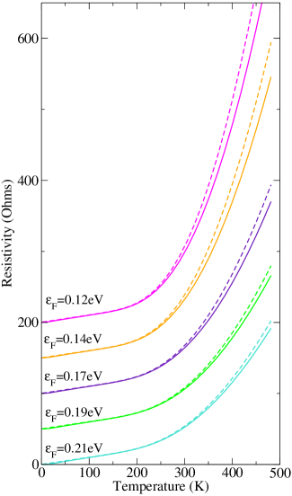
Figure 6: (Color online) Comparison between the full Boltzmann transport solution (plain lines) and the semi-analytical solution with the $\tau(\varepsilon_{\mathbf{k}})\approx\tau(\varepsilon_{\mathbf{k^{\prime}}})$ approximation made and the expressions of $\tau_{\nu}$ given in Sec. VIII.1 (dotted lines). Fitted EPC parameters were used. Residual resistivity was included in the transport simulation then subtracted for the plots. A fictitious residual resistivity was then added for clarity.

VIII.2 Additivity of resistivities

As shown in Sec. VIII.1, in the presence of impurities, it is possible to define independent times $\tau_{\nu}$ for each mode. Then from each time $\tau_{\nu}$, the resistivity $\rho_{\nu}$ of a given mode is obtained via the use of Eq. 61. It is then tempting to sum the resistivities to obtain the total resistivity. However, the energy integral of Eq. 61 should be carried on the total time $\tau$, found by adding the inverse times of each modes under Matthiessen’s rule. For the resistivities to be additive, it is required that

$$\tau=\left(\sum_{\nu}\frac{1}{\tau_{\nu}}\right)^{-1}\approx\sum_{\nu}\left(\frac{1}{\tau_{\nu}}\right)^{-1}$$ (68)

which is rarely valid, as demonstrated in Fig. 7. An important consequence is that care needs to be taken when the resistivity due to impurities (the so called residual resistivity) is subtracted from the overall resistivity to isolate the intrinsic contributions. This approach is justified only if the time $\tau_{\rm{I}}$ corresponding to impurities is such that $1/\tau_{\rm{I}}>>1/\tau_{\rm{A}}+1/\tau_{\rm{A}_{1}^{\prime}}+1/\tau_{\rm{O}}$. In general, this is not the case and impurity scattering have a more subtle effect than just shifting the total resistivity by $\rho_{\rm{I}}$ as shown in Fig. 7. Throughout this work, we include impurity scattering and then subtract the residual resistivity. This procedure is convenient but one must keep in mind that what remains is not the theoretical intrinsic resistivity. Both are plotted in Fig. 7, as well as Allen’s methodAllen (1978) used in our previous workPark et al. (2014). The latter overestimates the resistivity.

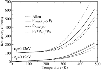
Figure 7: Comparison of various methods for the simulation of graphene’s resistivity. The complete solution to Boltzmann equation (including impurities) to which we subtract the residual resistivity $\rho_{\rm{I+A+A_{1}^{\prime}+O}}-\rho_{\rm{I}}$ gives the result closer to experimental conditions. The Boltzmann solution including only phonon contributions $\rho_{\rm{A+A_{1}^{\prime}+O}}$ corresponds to the theoretical intrinsic resistivity. The resistivity made up of the sum of independently derived resistivities is $\rho_{\rm{A}}+\rho_{\rm{A_{1}^{\prime}}}+\rho_{\rm{O}}$. Allen’s method, used on our previous workPark et al. (2014), overestimates the resistivity. Only at low temperature are those methods equivalent.

At low temperature, and in the EP regime, the process of adding the residual resistivity $\rho_{\rm{I}}(T=0)$ and the acoustic resistivity $\rho_{A}$ is justified and allows one to access directly the magnitude of gauge-field parameter $\beta_{A}$. Indeed, when only impurities and acoustic phonons contribute and if $\tau_{\rm{I}}<<\tau_{\rm{A}}$, the corresponding resistivities are additive. Moreover, in the EP regime, $\rho_{\rm{A}}$ has the simple expression (see appendix C for detailed derivation):

$$\rho_{A}\approx\frac{2\pi\beta_{A}^{2}k_{B}T}{e^{2}\hbar v_{F}^{2}\mu_{S}v_{\rm{A}}^{2}}\$$ (69)

It is clear that the slope of the resistivity is determined by $v_{\rm{A}}^{2}$ and $\beta^{2}_{A}$. Once the sound velocities are known, it is then possible to extract $\beta_{A}$ directly from transport measurements. We expect this parameter to be very close to the amplitude of the synthetic vector potential Low and Guinea (2010). One must be careful when comparing the result of such measurement to other values in literature. As noted in Ref. Perebeinos and Avouris, 2010, different EPC models bring different pre-factors in Eq. 69. For example, the magnitude of the deformation potential $D$ in Ref. Hwang and DasSarma, 2008 is defined such that a similar equation is obtained, but $D\equiv 2\beta_{A}$.

IX Conclusion

By diagonalizing the DFT dynamical matrix at finite phonon momentum, we developed a model for graphene’s acoustic phonon modes. Based on ab-initio simulations, we demonstrated that inserting those phonon modes into the most general symmetry-based model of electron-phonon interactions leads to numerically accurate values of acoustic gauge field parameter.
In order to calculate acoustic EPC parameters in the GW approximation, we developed a frozen phonon scheme based on strain deformations. We confirmed that the acoustic gauge field is renormalized by electron-electron interactions as the Fermi velocity.
We then showed that the scattering of electrons by acoustic phonons is mainly ruled by the unscreened gauge field while the deformation potential is strongly screened.
We developed a numerical solution to the complete Boltzmann transport equation including contributions from all phonon branches. Comparison to experiment confirm the role of acoustic phonons in the low temperature regime of resistivity. In the equipartition regime, the resistivity is proportional to $\frac{\beta^{2}_{A}}{v^{2}_{A}}$ and doping and substrate independent. We found that a $15\%$ increase of the acoustic gauge field parameter with respect to the GW value gives excellent agreement with experiment. In the high temperature regime, scattering by intrinsic A${}_{1}^{\prime}$ optical phonon modes could account for the strong increase in resistivity. However, a doping-dependent renormalization of the corresponding EPC parameter is necessary, and this renormalization is much stronger than existing estimate within GW. The role of remote-phonon scattering at high temperature was not ruled out. If remote-phonons are indeed involved, their screening plays an important role and needs to be modeled and simulated accurately.
We verified the validity of approximations commonly used in the solving of the Boltzmann transport equation. An approximate yet accurate semi-numerical solution is proposed. Finally, partial analytic solutions were derived in order to extract the numerical parameter (gauge field parameter) that relates the synthetic vector potential to strain directly from transport measurements.

Appendix A Numerical Solution to Boltzmann transport equation

Eq. LABEL:eq:BT1 can be written as a matrix-vector product of the kind $\sum_{\varepsilon^{\prime}}\mathcal{M}_{\varepsilon,\varepsilon^{\prime}}\tau(\varepsilon^{\prime})=1$, with $\mathcal{M}=\mathcal{M}_{\rm{I}}+\sum_{\nu}\mathcal{M}_{\nu}$ where $\mathcal{M}_{\rm{I}}$ is just a diagonal matrix containing the inverse relaxation times for impurity scattering obtained using existing methodsHwang et al. (2007); Hwang and Das Sarma (2008); Barreiro et al. (2009) and

$$\left[\mathcal{M}_{\nu}\right]_{\varepsilon,\varepsilon^{\prime}} = \sum_{\theta^{\prime}}\frac{|\varepsilon^{\prime}|\Delta\theta^{\prime}}{(2\pi\hbar v_{F})^{2}}P_{\nu}(\varepsilon,\theta,\varepsilon^{\prime},\theta^{\prime})\frac{1-f^{(0)}(\varepsilon^{\prime})}{1-f^{(0)}(\varepsilon)}$$ (70)

$$\left(\delta_{\varepsilon,\varepsilon^{\prime}}-\frac{\cos(\theta^{\prime})}{\cos(\theta)}\right)$$

where angular variables have been discretized with step $\Delta\theta^{\prime}$ to perform numerical integrals, $\theta=\theta_{\mathbf{k}}$ and $\theta^{\prime}=\theta_{\mathbf{k^{\prime}}}$. The scattering probability $P_{\nu}(\varepsilon,\theta,\varepsilon^{\prime},\theta^{\prime})$ is the equivalent of Eq. 56, defined in a way more suitable for the numerical integration:

$$P_{\nu}(\varepsilon,\theta,\varepsilon^{\prime},\theta^{\prime}) = \frac{2\pi}{\hbar}S_{\Re}|g_{\mathbf{k+q},\mathbf{k},\nu}|^{2}\left\{n_{q,\nu}\delta_{\varepsilon^{\prime},\varepsilon+\hbar\omega_{\mathbf{q},\nu}}\right.$$ (71)

$$+ \left.(n_{q,\nu}+1)\delta_{\varepsilon^{\prime},\varepsilon_{\mathbf{k}}-\hbar\omega_{\mathbf{q},\nu}}\right\}$$

We represent the matrix $\left[\mathcal{M}_{\nu}\right]_{\varepsilon,\varepsilon^{\prime}}$ by discretizing the energy bands with $N_{\mathcal{M}}=8000$ energy points on a scale of $E_{\mathcal{M}}=4\hbar\omega_{\rm{A}_{1}^{\prime}}$ around $\varepsilon_{F}$, such that $\Delta\varepsilon=\frac{E_{\mathcal{M}}}{N_{\mathcal{M}}}$. We sum over matrices associated with each phonon branch. The sum of scattering probabilities $P_{\rm{LO}}+P_{\rm{TO}}$ being isotropic, the corresponding matrix is diagonal. On the contrary, $P_{\rm{TA}}$, $P_{\rm{LA}}$ and $P_{A^{\prime}_{1}}$ have angular dependencies such that the term $\frac{\cos(\theta^{\prime})}{\cos(\theta)}$ does not integrate to zero and give rise to off-diagonal terms.

The number of off-diagonal terms in the matrix $\left[\mathcal{M}_{\nu}\right]_{\varepsilon,\varepsilon^{\prime}}$ depends of the energy conservation in the scattering probability, Eq. 56. In the small $|\mathbf{q}|$ limit and for optical A${}_{1}^{\prime}$ having constant long-wavelength phonon-dispersion, each energy conservation in Eq. 56 is satisfied for only one value of $\varepsilon$ at fixed phonon momentum. Thus, the matrix $\left[\mathcal{M}_{\rm{A}_{1}^{\prime}}\right]_{\varepsilon,\varepsilon^{\prime}}$ has only 2 off-diagonal terms for each $\varepsilon$. The energy parametrization is such that the energies $\varepsilon\pm\hbar\omega_{\rm{A}_{1}^{\prime}}$ are on the grid.

In the case of acoustic phonons, the linear phonon dispersion $\hbar\omega_{\mathbf{q},\nu}=v_{\nu}|\mathbf{q}|$ implies that the energy conservation in Eq. 56 is satisfied by a larger subset of $\varepsilon^{\prime}$ values for each $\varepsilon$. $\left[\mathcal{M}_{\rm{TA},\rm{LA}}\right]_{\varepsilon,\varepsilon^{\prime}}$ is thus a band matrix. However, the distance from the diagonal is given by the magnitude of the phonon frequency, and since $\hbar\omega_{\mathbf{q},\rm{TA}/\rm{LA}}\lesssim\hbar\omega_{2k_{F},\rm{LA}}=2\frac{v_{\rm{LA}}}{v_{F}}\varepsilon_{F}<<\hbar\omega_{\rm{A}_{1}^{\prime}}$, the band is very narrow compared to the width of the full matrix. For the acoustic modes only, we made the approximation that all of off-diagonal terms can be summed up and concentrated into the diagonal term, which is equivalent to neglectingHwang and DasSarma (2008) the variation of $\tau(\varepsilon)$ on the energy scale $\hbar\omega_{2k_{F},\rm{TA}/\rm{LA}}$. This approximation is discussed in App. B concerning the acoustic phonons in the BG regime. It is not equivalent to the elastic approximation, as in this case, we do not constrain $\varepsilon=\varepsilon^{\prime}$ in the calculation of each term in Eq. 70.
Matrix inversion of the $8000\times 8000$ $\mathcal{M}$ matrix gives the time $\tau(\varepsilon)$.

Appendix B Relaxation times

In this appendix, the $\tau(\varepsilon_{\mathbf{k^{\prime}}})\approx\tau(\varepsilon_{\mathbf{k}})$ approximation is made, such that each phonon mode can be treated separately. Some phonon-specific approximations can then be made to simplify the calculation of each $\tau_{\nu}$. In the following the indices $A$ and $O$ designate the summed contributions of acoustic (TA/LA) and optic (LO/TO) phonons, respectively.

B.1 Acoustic phonons in the BG regime:

The variation of $\tau_{\rm{A}}$ on the scale $\hbar\omega_{\mathbf{q},\rm{TA}/\rm{LA}}$ is neglected Hwang and DasSarma (2008). Since $\hbar\omega_{\mathbf{q},\rm{TA}/\rm{LA}}\ll\varepsilon_{F}$, the initial and final states can be considered to be on the same iso-energetic line at $\varepsilon=\varepsilon_{F}$, which simplifies the angular part of the calculus. However, the variation of the electronic occupation must be included because $\hbar\omega_{\mathbf{q},\rm{TA}/\rm{LA}}$ is of the order of $k_{B}T$. The following expression of $\tau_{\rm{A}}$ is found, with $\nu=\rm{TA},\rm{LA}$:

$$\left(\frac{1}{\tau_{\rm{A}}(\varepsilon_{\mathbf{k}})}\right)_{BG}=\sum_{\mathbf{k^{\prime}}}\frac{2\pi}{\hbar}\frac{1}{N}\sum_{\nu}|g_{\mathbf{k^{\prime}},\mathbf{k},\nu}|^{2}\frac{1-f^{(0)}(\mathbf{k^{\prime}})}{1-f^{(0)}(\mathbf{k})}$$ (72)

$$\times\big{\{}n_{|\mathbf{k^{\prime}}-\mathbf{k}|\nu}\delta(\varepsilon_{\mathbf{k^{\prime}}}-\varepsilon_{\mathbf{k}}-\hbar\omega_{|\mathbf{k}-\mathbf{k^{\prime}}|,\nu})$$

$$+(n_{|\mathbf{k}-\mathbf{k^{\prime}}|\nu}+1)\delta(\varepsilon_{\mathbf{k^{\prime}}}-\varepsilon_{\mathbf{k}}+\hbar\omega_{|\mathbf{k}-\mathbf{k^{\prime}}|,\nu})\big{\}}(1-\cos(\theta_{\mathbf{k^{\prime}}}-\theta_{\mathbf{k}}))$$

$S_{\Re}$ is the area of the real space unit-cell, $\mu_{S}$ is the mass density per unit area of graphene, and $\mathbf{k^{\prime}}=\mathbf{k}+\mathbf{q}$.

B.2 Acoustic phonons in the EP and HT regimes:

The quasi-elastic approximation is valid. The phonon occupation can be approximated as $n_{q,\rm{TA}/\rm{LA}}\approx\hbar\omega_{\mathbf{q},\rm{TA}/\rm{LA}}/(k_{B}T)$, since $k_{B}T>>\hbar\omega_{\mathbf{q},\rm{TA}/\rm{LA}}$. We use the following expression of $\tau_{\nu}(\varepsilon_{\mathbf{k}})$, easily deduced from Eq. 64 in the elastic case:

$$\frac{1}{\tau_{\nu}(\varepsilon_{\mathbf{k}})}=\sum_{\mathbf{k^{\prime}}}P_{\mathbf{k}\mathbf{k^{\prime}},\nu}\Big{(}1-\cos(\theta_{\mathbf{k^{\prime}}}-\theta_{\mathbf{k}})\Big{)}\ \ \text{(Elastic)}$$ (73)

The cosine in the scattering probabilities $P_{\mathbf{k}\mathbf{k^{\prime}},\rm{TA}/\rm{LA}}$ times the cosine in the above equation integrates to zero, so that $\frac{1}{\tau_{\rm{A}}(\varepsilon_{\mathbf{k}})}=\sum_{\nu=\rm{TA},\rm{LA}}\sum_{\mathbf{k^{\prime}}}P_{\mathbf{k}\mathbf{k^{\prime}},\nu}$. We finally obtain:

$$\left(\frac{1}{\tau_{\rm{A}}(\varepsilon_{\mathbf{k}})}\right)_{\rm{EP,HT}}=\frac{2\beta_{A}^{2}k_{B}T}{\mu_{S}\hbar v_{\rm{A}}^{2}}\frac{\varepsilon_{\mathbf{k}}}{(\hbar v_{F})^{2}}\\$$ (74)

Where $v_{\rm{A}}$ is the effective sound velocity defined in Eq. 66.

B.3 Optical LO/TO phonons:

The scattering probability made by the sum of LO and TO branches ($P_{\mathbf{k}\mathbf{k^{\prime}},\rm{LO}}+P_{\mathbf{k}\mathbf{k^{\prime}},\rm{TO}}$) is isotropic. We can use a simplified form of Eq. 62 in the isotropic case:

$$\frac{1}{\tau_{\nu}(\varepsilon_{\mathbf{k}})}=\sum_{\mathbf{k^{\prime}}}P_{\mathbf{k}\mathbf{k^{\prime}},\nu}\frac{1-f^{(0)}(\varepsilon_{\mathbf{k^{\prime}}})}{1-f^{(0)}(\varepsilon_{\mathbf{k}})}\ \ \text{(Isotropic)}$$ (75)

We obtain the following expression, with $\hbar\omega_{\rm{LO}}=\hbar\omega_{\rm{TO}}=\hbar\omega_{\rm{O}}=0.20$ eV, and $n_{\rm{LO}}=n_{\rm{TO}}=n_{\rm{O}}=n(\hbar\omega_{\rm{O}})$:

$$\frac{1}{\tau_{\rm{O}}(\varepsilon_{\mathbf{k}})}=\frac{\beta^{2}_{O}}{\mu_{S}\omega_{\rm{O}}}\frac{1}{(\hbar v_{F})^{2}}\big{\{}n_{\rm{O}}|\varepsilon_{\mathbf{k}}+\hbar\omega_{\rm{O}}|\frac{1-f^{(0)}(\varepsilon_{\mathbf{k}}+\hbar\omega_{\rm{O}})}{1-f^{(0)}(\varepsilon_{\mathbf{k}})}$$

$$+(n_{\rm{O}}+1)|\varepsilon_{\mathbf{k}}-\hbar\omega_{\rm{O}}|\frac{1-f^{(0)}(\varepsilon_{\mathbf{k}}-\hbar\omega_{\rm{O}})}{1-f^{(0)}(\varepsilon_{\mathbf{k}})}\big{\}}$$ (76)

B.4 Optical A${}_{1}^{\prime}$ phonons:

As mentioned before, a difficulty encountered with Optical A${}_{1}^{\prime}$ phonons at K is the change in the EPC matrix element for inter-band scattering. Since we consider only electron doping, inter-band scattering occurs only in case of phonon emission. We find the general expression of $\tau_{\rm{A}_{1}^{\prime}}$ to be, with $\hbar\omega_{\rm{A}_{1}^{\prime}}=0.15$ eV and $n_{\rm{A}_{1}^{\prime}}=n(\hbar\omega_{\rm{A}_{1}^{\prime}})$ :

$$\frac{1}{\tau_{\rm{A}_{1}^{\prime}}(\varepsilon_{\mathbf{k}})}=\frac{\beta^{2}_{K}}{\mu_{S}\omega_{\rm{A}_{1}^{\prime}}}\frac{1}{(\hbar v_{F})^{2}}$$ (77)

$$\times\ \ \left\{\frac{3}{2}n_{\rm{A}_{1}^{\prime}}|\varepsilon_{\mathbf{k}}+\hbar\omega_{\rm{A}_{1}^{\prime}}|\frac{1-f^{(0)}(\varepsilon_{\mathbf{k}}+\hbar\omega_{\rm{A}_{1}^{\prime}})}{1-f^{(0)}(\varepsilon_{\mathbf{k}})}\right.$$

$$\left.+(n_{\rm{A}_{1}^{\prime}}+1)\left(|\varepsilon_{\mathbf{k}}-\hbar\omega_{\rm{A}_{1}^{\prime}}|+\frac{1}{2}(\varepsilon_{\mathbf{k}}-\hbar\omega_{\rm{A}_{1}^{\prime}})\right)\right.$$

$$\ \ \left.\frac{1-f^{(0)}(\varepsilon_{\mathbf{k}}-\hbar\omega_{\rm{A}_{1}^{\prime}})}{1-f^{(0)}(\varepsilon_{\mathbf{k}})}\right\}$$

Appendix C Derivation of acoustic phonon resistivity in equipartition regime

In the EP regime, we can consider scattering by acoustic phonons ($\nu=\rm{TA},\rm{LA}$) to be elastic:

$$\frac{1}{\tau_{\rm{A}}(\varepsilon_{\mathbf{k}})}=\sum_{\nu}\sum_{\mathbf{k^{\prime}}}P_{\mathbf{k}\mathbf{k^{\prime}},\nu}\Big{(}1-\cos(\theta_{\mathbf{k^{\prime}}}-\theta_{\mathbf{k}})\Big{)}$$ (78)

with

$$P_{\mathbf{k}\mathbf{k^{\prime}},A} = \frac{2\pi}{\hbar}\frac{1}{N}\sum_{\nu}|g_{\mathbf{k},\mathbf{k^{\prime}},\nu}|^{2}\big{\{}n_{|\mathbf{k^{\prime}}-\mathbf{k}|\nu}\delta(\varepsilon_{\mathbf{k^{\prime}}}-\varepsilon_{\mathbf{k}}-\hbar\omega_{|\mathbf{k}-\mathbf{k^{\prime}}|,\nu})$$ (79)

$$+(n_{|\mathbf{k}-\mathbf{k^{\prime}}|\nu}+1)\delta(\varepsilon_{\mathbf{k^{\prime}}}-\varepsilon_{\mathbf{k}}+\hbar\omega_{|\mathbf{k}-\mathbf{k^{\prime}}|,\nu})\big{\}}$$

By neglecting the phonon frequency in the delta functions we obtain

$$P_{\mathbf{k}\mathbf{k^{\prime}},A}\approx\frac{2\pi}{\hbar}\frac{1}{N}\sum_{\nu}|g_{\mathbf{k},\mathbf{k^{\prime}},\nu}|^{2}\delta(\varepsilon_{\mathbf{k^{\prime}}}-\varepsilon_{\mathbf{k}})\big{\{}2n_{|\mathbf{k}-\mathbf{k^{\prime}}|\nu}+1\big{\}}$$

$$\approx\frac{2\pi}{\hbar}\frac{1}{N}\sum_{\nu=\rm{TA},\rm{LA}}\frac{\beta_{A}^{2}k_{B}T}{\mu_{S}S_{\Re}v_{\nu}^{2}}(1\pm\cos 3(\theta_{\mathbf{k^{\prime}}}+\theta_{\mathbf{k}}))\delta(\varepsilon_{\mathbf{k^{\prime}}}-\varepsilon_{\mathbf{k}})$$

where $|\mathbf{k}-\mathbf{k^{\prime}}|=|\mathbf{q}|$ and the angular expressions are simplified because $\mathbf{k^{\prime}}$ and $\mathbf{k}$ are on a iso-energetic line. The $\pm$ sign corresponds to $\rm{LA}$ and $\rm{TA}$ respectively. We made the approximation $n_{|\mathbf{q}|,\rm{TA}/\rm{LA}}\approx\frac{k_{B}T}{\hbar\omega_{\mathbf{q},TA/LA}}$, since $k_{B}T>>\hbar\omega_{\mathbf{q},TA/LA}$.

Thus we have:

$$\frac{1}{\tau(\varepsilon_{\mathbf{k}})} \approx \sum_{k^{\prime}}\frac{2\pi}{\hbar}\frac{1}{N}\sum_{\nu=\rm{TA},\rm{LA}}\frac{1}{\mu_{S}S_{\Re}v_{\nu}^{2}}\beta_{A}^{2}k_{B}T(1\pm\cos 3(\theta_{\mathbf{k^{\prime}}}+\theta_{\mathbf{k}}))\delta(\varepsilon_{\mathbf{k^{\prime}}}-\varepsilon_{\mathbf{k}})(1-\cos(\theta_{\mathbf{k^{\prime}}}-\theta_{\mathbf{k}}))$$ (80)

$$\frac{1}{\tau(\varepsilon_{\mathbf{k}})} \approx \sum_{\nu=\rm{TA},\rm{LA}}\frac{\beta_{A}^{2}k_{B}T}{\mu_{S}\hbar v_{\nu}^{2}}\frac{1}{(\hbar v_{F})^{2}}\int\frac{|\varepsilon_{\mathbf{k^{\prime}}}|d\varepsilon_{\mathbf{k^{\prime}}}d\theta_{\mathbf{k^{\prime}}}}{(2\pi)}(1\pm\cos 3(\theta_{\mathbf{k^{\prime}}}+\theta_{\mathbf{k}}))\delta(\varepsilon_{\mathbf{k^{\prime}}}-\varepsilon_{\mathbf{k}})(1-\cos(\theta_{\mathbf{k^{\prime}}}-\theta_{\mathbf{k}}))$$ (81)

$$\frac{1}{\tau(\varepsilon_{\mathbf{k}})} \approx \sum_{\nu=\rm{TA},\rm{LA}}\frac{\beta_{A}^{2}k_{B}T}{\mu_{S}\hbar v_{\nu}^{2}}\frac{|\varepsilon_{\mathbf{k}}|}{(\hbar v_{F})^{2}}\int\frac{d\theta_{\mathbf{k^{\prime}}}}{(2\pi)}(1\pm\cos 3(\theta_{\mathbf{k^{\prime}}}+\theta_{\mathbf{k}}))(1-\cos(\theta_{\mathbf{k^{\prime}}}-\theta_{\mathbf{k}}))$$ (82)

$$\frac{1}{\tau(\varepsilon_{\mathbf{k}})} \approx \frac{2\beta_{A}^{2}k_{B}T}{\mu_{S}\hbar v_{\rm{A}}^{2}}\frac{|\varepsilon_{\mathbf{k}}|}{(\hbar v_{F})^{2}}$$ (83)

Doing the usual approximation valid at low temperature:

$$\frac{1}{\rho} = \frac{e^{2}v_{F}^{2}}{2}\int d\varepsilon DOS(\varepsilon)\tau(\varepsilon)\left(-\frac{\partial f^{(0)}}{\partial\varepsilon}(\varepsilon)\right)$$ (84)

$$\approx \frac{e^{2}v_{F}^{2}}{2}DOS(\varepsilon_{F})\tau(\varepsilon_{F})\approx\frac{e^{2}v_{F}^{2}|\varepsilon_{F}|}{\pi(\hbar v_{F})^{2}}\tau(\varepsilon_{F})$$ (85)

we obtain:

$$\rho_{A} \approx\frac{\pi(\hbar v_{F})^{2}}{e^{2}v_{F}^{2}|\varepsilon_{F}|}\frac{1}{\tau(\varepsilon_{F})}$$ (86)

$$\rho_{A} \approx\frac{2\pi\beta_{A}^{2}k_{B}T}{e^{2}\hbar v_{F}^{2}\mu_{S}v_{\rm{A}}^{2}}$$ (87)

References

- Novoselov et al. (2005) K. S. Novoselov, A. K. Geim, S. V. Morozov, D. Jiang, M. I. Katsnelson, I. V. Grigorieva, S. V. Dubonos, and A. A. Firsov, Nature 438, 197 (2005).
- Zhang et al. (2005) Y. Zhang, Y.-W. Tan, H. L. Stormer, and P. Kim, Nature 438, 201 (2005).
- Das Sarma et al. (2011) S. Das Sarma, S. Adam, E. H. Hwang, and E. Rossi, Reviews of Modern Physics 83, 407 (2011).
- Avouris et al. (2007) P. Avouris, Z. Chen, and V. Perebeinos, Nature nanotechnology 2, 605 (2007).
- Chen et al. (2008) J. J.-H. Chen, C. Jang, S. Xiao, M. Ishigami, and M. S. Fuhrer, Nature Nanotechnology 3, 206 (2008).
- Efetov and Kim (2010) D. K. Efetov and P. Kim, Physical Review Letters 105, 256805 (2010).
- Pietronero et al. (1980) L. Pietronero, S. Strässler, H. R. Zeller, and M. J. Rice, Physical Review B 22, 904 (1980).
- Woods and Mahan (2000) L. M. Woods and G. D. Mahan, Physical Review B 61, 10651 (2000).
- Suzuura and Ando (2002) H. Suzuura and T. Ando, Physical Review B 65, 235412 (2002).
- Piscanec et al. (2004) S. Piscanec, M. Lazzeri, F. Mauri, A. C. Ferrari, and J. Robertson, Physical Review Letters 93, 185503 (2004).
- Manes (2007) J. L. Manes, Physical Review B 76, 045430 (2007).
- Samsonidze et al. (2007) G. G. Samsonidze, E. B. Barros, R. Saito, J. Jiang, G. Dresselhaus, and M. S. Dresselhaus, Physical Review B 75, 155420 (2007).
- Venezuela et al. (2011) P. Venezuela, M. Lazzeri, and F. Mauri, Physical Review B 84, 035433 (2011).
- Shishir and Ferry (2009) R. S. Shishir and D. K. Ferry, Journal of physics. Condensed matter : an Institute of Physics journal 21, 232204 (2009).
- Hwang and DasSarma (2008) E. H. Hwang and S. DasSarma, Physical Review B 77, 115449 (2008).
- Park et al. (2014) C.-H. Park, N. Bonini, T. Sohier, G. Samsonidze, B. Kozinsky, M. Calandra, F. Mauri, and N. Marzari, Nano letters 14, 1113 (2014).
- Borysenko et al. (2010) K. M. Borysenko, J. T. Mullen, E. A. Barry, S. Paul, Y. G. Semenov, J. M. Zavada, M. B. Nardelli, and K. W. Kim, Physical Review B 81, 121412 (2010).
- Kaasbjerg et al. (2012) K. Kaasbjerg, K. S. K. K. Thygesen, and K. K. W. Jacobsen, Physical Review B 85, 165440 (2012), arXiv:arXiv:1201.4661v1 .
- Allen (1978) P. B. Allen, Physical Review B 17, 3725 (1978).
- Hedin (1965) L. Hedin, Physical Review 139, A796 (1965).
- Perdew and Zunger (1981) J. P. Perdew and A. Zunger, Physical Review B 23, 5048 (1981).
- Giannozzi et al. (2009) P. Giannozzi, S. Baroni, N. Bonini, M. Calandra, R. Car, C. Cavazzoni, D. Ceresoli, G. L. Chiarotti, M. Cococcioni, I. Dabo, A. Dal Corso, S. de Gironcoli, S. Fabris, G. Fratesi, R. Gebauer, U. Gerstmann, C. Gougoussis, A. Kokalj, M. Lazzeri, L. Martin-Samos, N. Marzari, F. Mauri, R. Mazzarello, S. Paolini, A. Pasquarello, L. Paulatto, C. Sbraccia, S. Scandolo, G. Sclauzero, A. P. Seitsonen, A. Smogunov, P. Umari, and R. M. Wentzcovitch, Journal of physics. Condensed matter : an Institute of Physics journal 21, 395502 (2009), arXiv:arXiv:0906.2569v2 .
- Baroni et al. (2001) S. Baroni, S. de Gironcoli, and A. Dal Corso, Reviews of Modern Physics 73, 515 (2001), arXiv:0012092v1 [arXiv:cond-mat] .
- Deslippe et al. (2012) J. Deslippe, G. Samsonidze, D. A. Strubbe, M. Jain, M. L. Cohen, and S. G. Louie, Computer Physics Communications 183, 1269 (2012).
- Ismail-Beigi (2006) S. Ismail-Beigi, Physical Review B 73, 233103 (2006).
- Hybertsen and Louie (1986) M. S. Hybertsen and S. G. Louie, Physical Review B 34, 5390 (1986).
- Castro Neto et al. (2009) A. H. Castro Neto, F. Guinea, N. M. R. Peres, K. S. Novoselov, and A. Geim, Reviews of Modern Physics 81, 109 (2009).
- von Oppen et al. (2009) F. von Oppen, F. Guinea, and E. Mariani, Physical Review B 80, 075420 (2009).
- Vozmediano et al. (2010) M. Vozmediano, M. Katsnelson, and F. Guinea, Physics Reports 496, 109 (2010).
- Guinea et al. (2010) F. Guinea, A. K. Geim, M. I. Katsnelson, and K. S. Novoselov, Physical Review B 81, 035408 (2010).
- Lazzeri et al. (2008) M. Lazzeri, C. Attaccalite, L. Wirtz, and F. Mauri, Physical Review B 78, 081406 (2008).
- Attaccalite et al. (2010) C. Attaccalite, L. Wirtz, M. Lazzeri, F. Mauri, and A. Rubio, Nano letters 10, 1172 (2010).
- Choi et al. (2010) S.-M. Choi, S.-H. Jhi, and Y.-W. Son, Physical Review B 81, 081407 (2010).
- Ando (2006) T. Ando, Journal of the Physics Society Japan 75, 074716 (2006).
- Hwang and Das Sarma (2007) E. H. Hwang and S. Das Sarma, Physical Review B 75, 205418 (2007), arXiv:0610561v3 [arXiv:cond-mat] .
- Note (1) Note that the DFPT values of are overall much smaller than this estimation. However, this is expected since refers to an isolated single layer of graphene whereas our DFPT calculations are performed in a multilayered system where the graphene planes are separated by Å. For the phonon momenta considered in the paper, the screening from the periodic images is not negligible at all. Indeed, a phonon of wavevector induces a charge fluctuation with a periodicity equal to . The electric field induced by such a charge fluctuation decays exponentially, along the out-of-plane direction, on a typical length scale of . Therefore, for the interlayer distance of Å used in our calculations, the electric field induced by the periodic images is negligible only for much larger than Å-1 Å-1. Such requirement is not satisfied by our DFPT calculations where is in the range Å-1. The deformation potential is thus over-screened in our DFPT calculations with respect to the isolated single layer case.
- Note (2) Strictly speaking, for graphene very close to charge neutrality, there is a logarithmic singularity in the group velocity near the Dirac point. We do not consider this effect here. By neutral graphene, we mean doping levels very low compared to those mentionned in the text, but high enough that the logarithmic singularity can be neglected.
- Basko and Aleiner (2008) D. M. Basko and I. L. Aleiner, Phys. Rev. B 77, 41409 (2008).
- Perebeinos and Avouris (2010) V. Perebeinos and P. Avouris, Physical Review B 81, 195442 (2010).
- Mariani and von Oppen (2010) E. Mariani and F. von Oppen, Physical Review B 82, 195403 (2010), arXiv:arXiv:1008.1631v1 .
- Hwang et al. (2007) E. H. Hwang, S. Adam, and S. DasSarma, Physical Review Letters 98, 186806 (2007).
- Ashcroft and Mermin (1976) N. W. Ashcroft and N. D. Mermin, Solid State Physics (Brooks Cole, Belmont (USA), 1976) p. 848.
- Nag (1980) B. Nag, Springer Series in Solid-State Sciences Springer Series in Solid-State Sciences, 11 (1980), 10.1007/978-3-642-81416-7.
- Kawamura and Das Sarma (1992) T. Kawamura and S. Das Sarma, Physical Review B 45, 3612 (1992).
- Basu and Nag (1980) P. K. Basu and B. R. Nag, Physical Review B 22, 4849 (1980).
- Hwang and Das Sarma (2008) E. H. Hwang and S. Das Sarma, Physical Review B 77, 195412 (2008).
- Barreiro et al. (2009) A. Barreiro, M. Lazzeri, J. Moser, F. Mauri, and A. Bachtold, Physical Review Letters 103, 76601 (2009).
- Das Sarma and Hwang (2013) S. Das Sarma and E. H. Hwang, Physical Review B 87, 035415 (2013).
- Martin et al. (2007) J. Martin, N. Akerman, G. Ulbricht, T. Lohmann, J. H. Smet, K. von Klitzing, and A. Yacoby, Nature Physics 4, 144 (2007).
- Hwang and Das Sarma (2009) E. H. Hwang and S. Das Sarma, Physical Review B 79, 165404 (2009).
- Dean et al. (2010) C. R. Dean, A. F. Young, I. Meric, C. Lee, L. Wang, S. Sorgenfrei, K. Watanabe, T. Taniguchi, P. Kim, K. L. Shepard, and J. Hone, Nature nanotechnology 5, 722 (2010).
- Zou et al. (2010) K. Zou, X. Hong, D. Keefer, and J. Zhu, Physical Review Letters 105, 126601 (2010).
- Matthiessen and Vogt (1864) A. Matthiessen and C. Vogt, Philosophical Transactions of the Royal Society of London 154, 167 (1864).
- Low and Guinea (2010) T. Low and F. Guinea, Nano letters 10, 3551 (2010).