Onset of plane layer magnetoconvection at low Ekman number

Abstract

We study the onset of magnetoconvection between two infinite horizontal planes subject to a vertical magnetic field aligned with background rotation. In order to gain insight into the convection taking place in the Earth’s tangent cylinder (TC), we target regimes of asymptotically strong rotation. The critical Rayleigh number $Ra_{c}$ and critical wavenumber are computed numerically by solving the linear stability problem in a systematic way. A parametric study is conducted, varying the Ekman number, $E$ (ratio of viscous to Coriolis forces) and the Elsasser number, $\Lambda$ (ratio of the Lorentz force to the Coriolis force). $E$ is varied from $10^{-9}$ to $10^{-2}$ and $\Lambda$ from $10^{-3}$ to $1$. Apply to arbitrary thermal and magnetic Prandtl numbers, our results verify and confirm previous experimental and theoretical results showing the existence of two distinct unstable modes at low values of $E$ – one being controlled by the magnetic field, the other being controlled by viscosity (often called the viscous mode). Asymptotic scalings for the onset of these modes have been numerically confirmed and precisely quantified. We show that with no-slip boundary conditions, the asymptotic behaviour is reached for $E<10^{-6}$ and establish a map in the $(E,\Lambda)$ plane. We distinguish regions where convection sets in either in the magnetic mode or in the viscous mode. Our analysis gives the regime in which the transition between magnetic and viscous modes may be observed. We also show that within the asymptotic regime, the role played by the kinematic boundary conditions is minimal.

I Introduction

In this paper, we analyse the onset of plane-layer convection governed by the interplay between the magnetic (Lorentz), buoyancy and Coriolis forces, to obtain an insight into how convection in the Tangent Cylinder (TC) region of the Earth’s liquid core is driven. This region is bounded by the Earth’s solid inner core at its bottom, the mantle at its top, and by an imaginary cylinder tangent to the solid inner core and parallel to the Earth’s rotation axis. Intense convection, compositional and thermal, is believed to take place in this region, affecting the structure of the magnetic field near the poles [sreenivasan2006azimuthal, ]. The Earth’s self-generated magnetic field is thought to affect the structure of convective cells in the TC, producing strong anticyclonic polar vortices that show up in the secular variation of the geomagnetic field [05grl, ]. The aim of our study is to find out whether onset of convection is sensitive to the Lorentz force in the regime of strong rotation that characterises the Earth.

Previous work on plane rotating magnetoconvection has been motivated either by geophysical or engineering applications involving liquid metals [burr2001rayleigh, ; busse1982stability, ; cioni2000effect, ; houchens2002rayleigh, ; takashima1999buoyancy, ; volz1999thermoconvective, ; yanagisawa2013convection, ]. A number of geophysically motivated studies focused on the dynamics outside the TC: an early study [fearn1979thermally, ] derived theoretical scalings for the critical Rayleigh number and wave number at the onset of convection as a function of the magnetic field intensity and magnitude of the Coriolis force. Other studies [busse1970thermal, ; busse1982stability, ; carrigan1983experimental, ] showed experimentally and theoretically that, in this region convection and rotation generated tall columns parallel to the rotation axis. A recent study investigated the role of a dipolar magnetic field in enhancing helicity in convection columns [sreenivasan2011helicity, ], which can explain subcritical behaviour as well as the preference for the axial dipole in rapidly rotating dynamos. These studies, however, do not consider the particularity of the TC, which, though imaginary, acts somewhat as a physical boundary because the presence of the solid inner core makes overcoming the Taylor-Proudman constraint more difficult. When convection does set in, motions vary strongly along $z$ as heat and composition flux have a substantial component in the $z$-direction. Due to the large aspect ratio of the TC, the curvature of the top and the bottom boundaries are not expected to play a lead role, at least at the onset of convection. On these grounds, a simple plane geometry is expected to provide a fair, albeit simplistic, representation of the TC. In this geometry, it was theorised [chandrasekhar1961hydrodynamic, , podvigina2010stability, ] and experimentally observed [nakagawa1957experiments, ] that the convection could set off through an instability either of a magnetic or a viscous mode, depending on the values of the Ekman number (Viscous to Coriolis forces) and of the Elsasser number (Lorentz to Coriolis forces). While the magnetic mode has a low horizontal wavenumber, the viscous mode is characterised by thin structures of high horizontal wavenumber parallel to the rotation axis. One would expect that convective flows driven by these two mechanisms to differ significantly. These studies showed that transition between these modes resulted in a brutal change in the wavelength of the observed convective pattern, but concerned only large values of $E$ ($>10^{-5}$). Such values may be too far from the asymptotic regimes relevant to the Earth’s ($E\sim 10^{-14}$) [gubbins2001rayleigh, ] to be applicable to it.

There have been experimental studies dedicated to the dynamics of the TC for $E=10^{-3}$ [aurnou2001experiments, ; aurnou2003experiments, ], but in the absence of the magnetic field, only the viscous mode of convection could be observed. The link between plane layer magnetoconvection and convection in the Earth’s TC was first established by linear onset calculations as well as numerical simulations of the geodynamo [05grl, ; sreenivasan2006azimuthal, ], where substantial thickening of buoyant plumes under the effect of the magnetic field was noted, albeit at values of $E$ down to $10^{-4}$ only. Crucially, these studies showed that non-axisymmetric, Earth-like polar vortices are obtained only through the action of the magnetic field.

To explore Earth-relevant regimes, we look at plane-layer magnetoconvection at values of $E$ low enough to find an asymptotic regime. Although actual regimes of the TC remain beyond the reach of this analysis, asymptotic scalings are relevant to it. In the same spirit, we shall characterise the consequence of using either a no-slip boundary condition or its less computationally demanding stress-free counterpart on these regimes.

The paper is organised as follows: Section 2 introduces the governing equations and the numerical method to solve them is validated. Results are discussed in Section 3 results and scalings for the asymptotic regimes are expressed in terms of $E$ and $\Lambda$. Relevance to the Earth is discussed in section 4.

II Governing Equations and Numerical Method

II.1 Governing equations

We consider an incompressible fluid (viscosity $\nu$, thermal diffusivity $\kappa$, magnetic diffusivity $\eta$, density $\rho$, expansion coefficient $\alpha$) confined between two differentially heated infinite horizontal plane boundaries, separated by a distance $d$. The temperature difference between them is $\Delta T$. The flow rotates at a speed $\Omega$ around the vertical axis $\mathbf{z}$ and is permeated by a uniform vertical magnetic field $\mathbf{B}=B_{0}\mathbf{e_{z}}$. Figure 1 illustrates our geometry.

Figure 1: Schematic illustration of the geometry

The flow is governed by the full incompressible MHD equations under the Boussinesq approximation. Normalising lengths by $d$, the velocity by $\eta/d$, the pressure by $\rho\eta\Omega$, the magnetic field by $B_{0}$, the time by $d^{2}/\eta$, the temperature by $\Delta T$ and the rotation speed by $\Omega$, the equations can be written in non-dimensional form, as follows:

$$P\!m^{-1}E(\frac{\partial\mathbf{u}}{\partial t}+(\mathbf{u}\cdot\bm{\nabla})\mathbf{u})+2\mathbf{\hat{z}}\times\mathbf{u}=-\bm{\nabla}p+R\!aT+\Lambda(\mathbf{\bm{\nabla}}\times\mathbf{B})\times\mathbf{B}+E\nabla^{2}\mathbf{u},$$ (1)

$$\frac{\partial\mathbf{B}}{\partial t}=\bm{\nabla}\times(\mathbf{u}\times\mathbf{B})+\nabla^{2}\mathbf{B},$$ (2)

$$\frac{\partial T}{\partial t}+(\mathbf{u}\cdot\bm{\nabla})T=P\!mP\!r^{-1}\nabla^{2}T,$$ (3)

$$\mathbf{\mathbf{\bm{\nabla}}}\cdot\mathbf{u}=0,$$ (4)

$$\bm{\nabla}\cdot\mathbf{B}=0,$$ (5)

where $\mathbf{B}$ is the total magnetic field. The system is controlled by 5 non-dimensional parameters: the Ekman number, $E=\nu/\Omega d^{2}$, a modified Rayleigh number, $R\!a=g\alpha\Delta Td/\eta\Omega$, the Elsasser number, $\Lambda=B^{2}/\mu_{0}\eta\rho\Omega$, the Prandtl number, $P\!r=\nu/\kappa$ and the magnetic Prandtl number, $P\!m=\nu/\eta$. We applied two different kinds of boundary conditions: stress-free magnetic (SFM) (conditions (6)– (9) below) and no-slip magnetic (NSM) (conditions (8)– (10) below). These are given respectively for $z=\pm 1/2$ as:

$$u_{z}=0\quad\mathrm{\text{(impermeability)},}$$ (6)

$$\dfrac{d^{2}u_{z}}{dz^{2}}=0\quad\mathrm{\text{(stress-free)}},$$ (7)

$$(\bm{\nabla}\times\mathbf{B}).\mathbf{e_{z}}=0\quad\mathrm{\text{(electrically insulating)},}$$ (8)

$$T(z=-1/2)=1,\;T(z=+1/2)=0,$$ (9)

$$\mathbf{u}=0\quad\mathrm{\text{(no-slip)}.}$$ (10)

For both sets of boundary conditions, the system has a simple solution with $\mathbf{u}_{0}=0$, $\mathbf{B}_{0}=0$, and $T=T_{0}+z\Delta T$. We are interested in the linear stability of this basic state. The problem’s invariance in the $x$ and $y$ directions allows us to decompose all physical quantities as $g(z)=g_{0}+\hat{g}(z)e^{i\mathbf{a}.\mathbf{r}_{\perp}}$, where $\mathbf{r}_{\perp}=(x,y)$ and $\mathbf{a}$ is the wave number. Following Sreenivasan & Jones [sreenivasan2006azimuthal, ], we shall only seek the shape of the unstable modes, not their growth rate. The perturbation equations in steady state are given by

$$E(D^{2}-a^{2})\hat{\omega_{z}}+2D\hat{u_{z}}+\Lambda D\hat{j_{z}}=0,$$ (11)

$$E(D^{2}-a^{2})^{2}\hat{u_{z}}-2D\hat{\omega_{z}}+\Lambda(D^{2}-a^{2})D\hat{b_{z}}-2R\!a\hat{T^{\prime}}=0,$$ (12)

$$(D^{2}-a^{2})\hat{b_{z}}+D\hat{u_{z}}=0,$$ (13)

$$(D^{2}-a^{2})\hat{j_{z}}+D\hat{\omega_{z}}=0,$$ (14)

$$P\!mP\!r^{-1}(D^{2}-a^{2})\hat{T^{\prime}}+\hat{u_{z}}=0.$$ (15)

Here $D$ is the derivative along $\mathbf{z}$, $\hat{\omega_{z}}$, $\hat{u_{z}}$, $\hat{j_{z}}$ and $\hat{b_{z}}$ are the $z$-components of the vorticity, velocity, electric current and magnetic field perturbations and $\hat{T^{{}^{\prime}}}$ is the temperature perturbation. The nondimensional wave number is denoted by $a=\parallel\mathbf{a}\parallel$. Eq. $(\ref{eq:-7})$ is obtained from $\bm{\nabla}\times(\ref{eq:})\cdot\mathbf{e_{z}}$, $(\ref{eq:-8})$ from $\bm{\nabla}\times[\bm{\nabla}\times(\ref{eq:})]\cdot\mathbf{e_{z}}$, $(\ref{eq:-9})$ from $\bm{\nabla}\times(\ref{eq:-1}).\mathbf{e_{z}}$, $(\ref{eq:-10})$ as $\bm{\nabla}\times[\bm{\nabla}\times(\ref{eq:-1})]\cdot\mathbf{e_{z}}$ and Eq. $(\ref{eq:-11})$ follows from Eq. $(\ref{eq:-2})$. The boundary conditions $(\ref{eq:condi1})$–$(\ref{eq:condi5})$ take the form

$$D^{2}\hat{u_{z}}=\hat{u_{z}}=D\hat{\omega_{z}}=\hat{j_{z}}=\hat{T^{\prime}}=0\quad\mathrm{for}\quad z=\pm 1/2,\quad(\mathrm{SFM})$$ (16)

$$D\hat{u_{z}}=\hat{u_{z}}=\hat{\omega_{z}}=\hat{j_{z}}=\hat{T^{\prime}}=0\quad\mathrm{for}\quad z=\pm 1/2\>.\quad(\mathrm{NSM})$$ (17)

The problem becomes a generalized eigenvalue problem of the form $AX=RaBX$. The critical Rayleigh number for the onset of convection $R\!a_{c}$ is found as an eigenvalue of the problem for any given $a$ and minimised over $a$ as in [chandrasekhar1961hydrodynamic, ]. With help of a formal transformation of $\hat{T^{\prime}}$ as $\hat{T_{m}^{\prime}}=P\!mP\!r^{-1}\hat{T^{\prime}}$ and $R\!a_{c}$ as $R\!a_{cm}=P\!rP\!m^{-1}R\!a_{c}$, the solution of this model is made independent of the magnetic and thermal diffusivities. The results presented there after therefore extend to arbitrary values of $P\!m$ and $P\!r$.

II.2 Numerical method

Eqs. $(\ref{eq:-7})-(\ref{eq:-11})$ were solved numerically using a spectral collocation method based on Chebyshev polynomials [schmid2001stability, ]. In the no-slip case, a boundary layer of thickness $\delta=2\sqrt{E\pi}$ develops along the walls [1973RPPh…36..159A, ], and we have ensured that at least 3 collocations points were in it. Some convergence tests have been performed to ensure that the resolution is adequate. The results are presented in figure 2, where we varied the number of collocations points $N$ between $5$ to $3000$. In the SFM case, the tests were performed for $\Lambda=1,\quad E=10^{-9}\quad\mathrm{and}\quad a=3.149$. NSM conditions were tested with $\Lambda=1,\quad E=10^{-7}\quad\mathrm{and}\quad a=3.333$. We chose these parameters to ensure a good convergence at the lowest $E$ we investigated. We look at the value of the error, $\epsilon$ on $R\!a_{c}$ relative to its value obtained for $N=3000$. For both types of boundary conditions, $N>100$ gives a small relative error. On the basis of this test, the results presented in the next section have been obtained with $N=600$ for the SFM case and $N=1200$ for the NSM case.

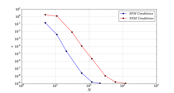
Figure 2: Convergence test

We performed a parametric study with $a=\left[1,1500\right]$, $E=\left[10^{-9},10^{-2}\right]$ and $\Lambda=\left[10^{-3},2\right]$ for SFM and $a=\left[1,1500\right]$, $E=\left[10^{-8},10^{-2}\right]$ and $\Lambda=\left[10^{-3},2\right]$ for NSM.

III Results

III.1 General properties

In figure 3, we illustrate the typical behaviour of the critical Rayleigh number, $R\!a_{c}$ with respect to the wave number, $a$. The blue curve corresponds to $E=10^{-8}$ and $\Lambda=1$. The green curves were obtained for $E=10^{-8}$ and $\Lambda=10^{-1}\;\mathrm{to}\;10^{-3}$ and the red curves for $E=10^{-5}\;\mathrm{to}\;10^{-7}$ at $\Lambda=1$. For each case, we note three specific values for $R\!a_{c}$. The first is a minimum occurring at low $a$, its position and value depends hardly on $E$ but is mostly controlled by $\Lambda$. As such, it is referred to as the magnetic mode which we shall denote $(R\!a_{c}^{m},\;a_{c}^{m})$, with $R\!a_{c}^{m}$ the magnetic critical Rayleigh number and $a_{c}^{m}$ the magnetic critical wave number. The second is a local minimum for relatively high $a$, its position and value depending essentially on $E$. We shall refer to it as the viscous mode $(R\!a_{c}^{v},\;a_{c}^{v})$, with $R\!a_{c}^{v}$ the viscous critical Rayleigh number and $a_{c}^{v}$ the viscous critical wave number. Both these modes were first identified by Chandrasekhar [chandrasekhar1961hydrodynamic, ]. The third feature is a local maximum located between the two previous modes. We call this the intermediate maximum and denote it by $(R\!a_{c}^{int},\;a_{c}^{int})$. The corresponding mode is always more stable than both the magnetic and the viscous mode and does not reflect any mechanism driving convection. At low $E$, the value of $R\!a_{c}^{int}$ is several orders of magnitude higher than $R\!a_{c}^{v}$ and $R\!a_{c}^{m}$. The intermediate maximum gives a measure of how much of a separation exists between magnetically controlled modes and modes controlled by viscosity.

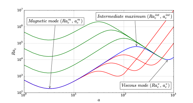
Figure 3: Variation of $R\!a_{c}$ with $a$. The blue curve’s input parameters are $E=10^{-8}$ and $\Lambda=1$. The red curve’s input parameters are $E=10^{-8}$ and $\Lambda=10^{-1}\;\mathrm{to}\;10^{-3}$. The green curve’s input parameters are $E=10^{-5}\;\mathrm{to}\;10^{-7}$ at $\Lambda=1$.

III.2 Scalings for the critical wavelength and Rayleigh number

In figures 4a and 4b, we show the variations of $R\!a_{c}$ and $a_{c}$ with $E$ at $\Lambda=[0.1,0.3,1,2]$ for the viscous mode, magnetic mode and for the intermediate maximum identified in $\mathbf{A}$, with SFM boundary conditions. We note two important results in the limit of $E\rightarrow 0$. Firstly, the scalings obtained for the viscous modes reproduce the classical results of nonmagnetic convection, that is, $R\!a_{c}^{v}\propto E^{-1/3}$ and $a_{c}^{v}\propto E^{-1/3}$; and for the intermediate maximum, $R\!a_{c}^{int}\propto E^{-1/2}$ and $a_{c}^{int}\propto E^{-1/4}$. Secondly, at low $E$, convection is initiated by the instability of the magnetic mode. On the other hand, when $E$ increases at a fixed value of $\Lambda$, $R\!a_{c}^{v}$ decreases while $R\!a_{c}^{m}$ remains constant, so that a crossover value $E_{c}(\Lambda)$ exists beyond which the viscous mode is more unstable than the critical one, and triggers the onset of convection. Before this point is reached, the clear separation between magnetic and viscous progressively starts disappearing. Ultimately, the intermediate maximum merges into the magnetic mode, at which point both disappear, for $E=E_{D}<E_{c}(\Lambda)$.

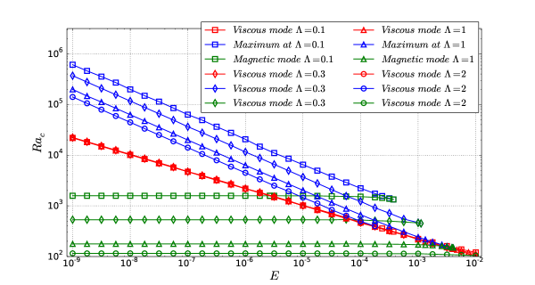
(a)

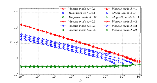
(b)

Figure 4: Variation of critical Rayleigh number, $R\!a_{c}$ (a) and critical wave number, $a_{c}$ (b) with Ekman number, $E$, for SFM boundary conditions.

In figure 5a and 5b, we report the variations of $R\!a_{c}^{m}$, $R\!a_{c}^{int}$, $R\!a_{c}^{v}$, $a_{c}^{m}$, $a_{c}^{int}$, and $a_{c}^{v}$ with $\Lambda$ for $E=10^{-8}$ and $E=10^{-7}$. The Elsasser number, $\Lambda$ has been restricted to values below $1$ which are relevant to the Earth’s core. For higher values of the Elsasser number, Sreenivasan and Jones [sreenivasan2006azimuthal, ] showed that the Lorentz force had a stabilising effect on the flow so that $R\!a_{c}^{m}(\Lambda)$ increases instead of decreasing as it does for $\Lambda<1$. In the limit of $\Lambda\rightarrow 0$, we observe that the intermediate maximum scales as as $R\!a_{c}^{int}\propto\text{$\Lambda$}^{-1/2}$ and $a_{c}^{int}\propto\Lambda^{1/4}$. For the magnetic mode, on the other hand, $R\!a_{c}^{m}\propto\Lambda^{-1}$ so that the separation between magnetic and viscous modes becomes more and more pronounced as $\Lambda$ increases. Interestingly, $a_{c}^{m}$ is practically independent of $\Lambda$ and $E$. The crossover point at which the magnetic mode becomes more unstable than the viscous mode can also be seen.

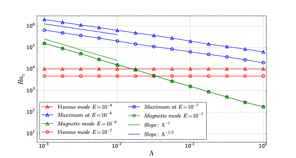
(a)

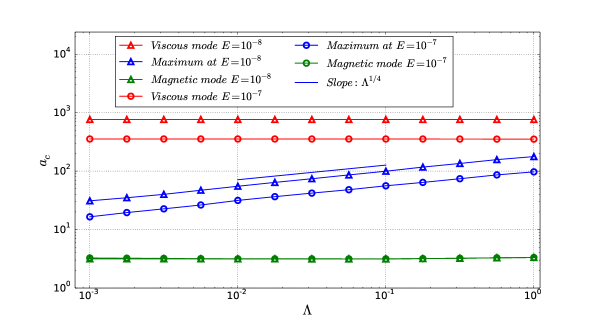
(b)

Figure 5: Variation of critical Rayleigh number, $R\!a_{c}$ (a) and critical wave number, $a_{c}$ (b) with Elsasser number, $\Lambda$, for SFM boundary conditions.

Figures 6a, 6b and 7a, 7b present the counterparts of Figures 4a, 4b and 5a, 5b for the problem with NSM boundary conditions. They indicate that the qualitative behaviour of the critical Rayleigh numbers and the critical wave numbers remains the same as in the configuration with SFM. In particular, the scalings for $R\!a_{c}$ and $a_{c}$ in the limit $E\rightarrow 0$ and $\Lambda\rightarrow 0$ remain valid.

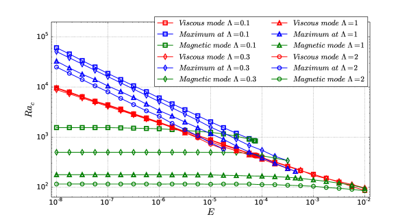
(a)

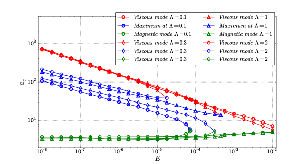
(b)

Figure 6: Variation of critical Rayleigh number, $R\!a_{c}$ (a) and critical wave number, $a_{c}$ (b) with Ekman number, $E$, for NSM boundary conditions.

These results corroborate the findings of Sreenivasan and Jones [sreenivasan2006azimuthal, ] that the boundary conditions at $z=-1/2$ and $z=+1/2$ have little influence on the onset of convection in these limits. One important difference between the two configurations, however, is that convergence towards the asymptotic scalings is significantly slower with NSM boundary conditions than with SFM boundary conditions (with a typical difference of two decades in $E$ and one decade in $\Lambda$). With SFM boundary conditions, at high $E$ and for $\Lambda=1$, the intermediate maximum merges with the viscous mode rather than with the magnetic mode. This behaviour can be expected to take place with NSM boundary conditions too since the wavenumbers of all three modes become closer to each other as $\Lambda$ increases. Our results confirm the relevance of the problem with SFM boundary conditions to the more realistic problem with NSM boundary conditions. The small influence of the boundaries comes as a useful feature given that simulations with NSM boundary conditions are considerably more computationally expensive than those with SFM boundary conditions.

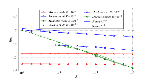
(a)

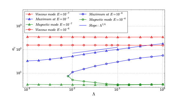
(b)

Figure 7: Variation of critical Rayleigh number, $R\!a_{c}$ (a) and critical wave number, $a_{c}$ (b) with Elsasser number, $\Lambda$, for NSM boundary conditions.

III.3 Parametric study in the $(\Lambda,E)$ space

Figures 8 and 9 map the mechanisms responsible for the onset of convection in the $(\Lambda,E)$ space. The blue squares represent the area in which only the viscous mode exists. The green triangles characterise the range of parameters where magnetic and viscous modes are present but the most unstable is the viscous one. Finally, the red circles correspond to regimes both magnetic and viscous modes are present but where the magnetic mode is more unstable than the viscous mode. In both figures, we draw two lines, one marked with red triangles and the other marked with blue triangles. These lines indicate respectively the merging of the intermediate maximum with the magnetic mode ($R\!a_{c}^{m}=R\!a_{c}^{int}$) and the crossover line where $R\!a_{c}^{v}=R\!a_{c}^{int}$. In the limit of $E\rightarrow 0$, these respectively obey the scalings:

$$\Lambda=270E,$$ (18)

and

$$\Lambda=7.22E^{1/3}.$$ (19)

Exponents in these laws readily follow from the scalings for $R\!a_{c}^{m}$, $R\!a_{c}^{v}$ and $R\!a_{c}^{int}$ obtained earlier. These results are observed for both types of boundary conditions. In the NSM case, however, this asymptotic behaviour becomes only apparent for $E\sim 10^{-5.5}$. In other words, the scaling observed at moderate $E$ with SFM boundary conditions reflects that with NSM at very low values of $E$. Furthermore, the fact that the shape of the curve $R\!a_{c}(a)$ is independent of the diffusivities $\kappa$ and $\eta$ allows us to mark out the area of parameters investigated in experiments [nakagawa1957experiments, ; aurnou2001experiments, ]. In particular, the experiments of [aurnou2001experiments, ] operates outside the viscous-magnetic transition ; which explains why these authors did not observe this phenomenon, while [nakagawa1957experiments, ] did. In any case, none of these experiments appear to have reached asymptotic regime of low $E$.

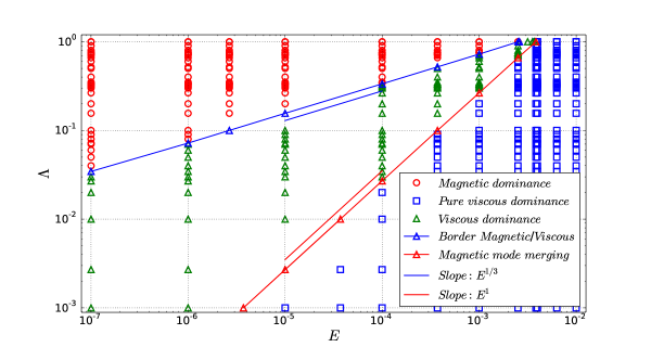
Figure 8: Characterisation of modes in the $(\Lambda,E)$ space with Stress-free Magnetic (SFM) conditions.

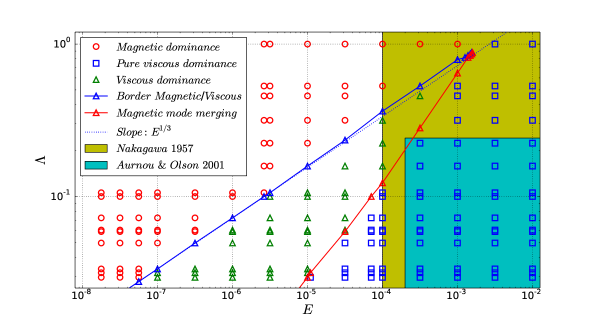
Figure 9: Characterisation of modes in the $(\Lambda,E)$ space with No-Slip Magnetic (NSM) conditions.

IV Discussion

In this work, we have presented a detailed parametric study of the linear stability problem governing the onset of plane magnetoconvection down to asymptotic regimes in the limit $E\rightarrow 0$. This led us to the following results:

1. We were able to precisely verify and quantify the theoretical scalings for the onset of the magnetic and the viscous convection modes, $Ra_{c}^{m}=\Lambda^{-1}$ and $Ra_{c}^{v}=E^{-1/3}$, for both NSM and SFM boundary conditions.

2. Our parametric analysis led us to establish a map in the space of parameters $(E,\Lambda)$ and to distinguish three regions: one where only the viscous mode exists, one where both viscous and magnetic modes exist but the magnetic mode is more unstable, and one where both exist but the viscous mode is more unstable. The crossover between instabilities due to the magnetic mode and instabilities due to the viscous one occurs for $\Lambda$=$7.22$$E^{1/3}$ in the limit $E\rightarrow 0$, in agreement with Sreenivasan and Jones [sreenivasan2006azimuthal, ].

3. With NSM, this asymptotic behaviour is only recovered for $E\sim 10^{-5.5}$ and this explains why the magnetic/viscous transition was observed in the experiments of Nakagawa [nakagawa1957experiments, ] and not in those of Aurnou & Olson [aurnou2001experiments, ].

4. This asymptotic behaviour is recovered both for SFM and NSM boundary conditions, but attained at much lower values of $E$ for the latter than the former. This implies that the asymptotic behaviour found at low $E$ with NSM is well reproduced with SFM boundary conditions and $E$ as high as $10^{-3}$.

Using values of $\Lambda$ between $0.08$ and $1$, $E=10^{-14}$ [davidson2013turbulence, ] and accepting the relevance of our simplified geometry, our results suggest that the onset of the convection inside the Earth’s TC is magnetically controlled. In the same way, our analysis can be applied to Mercury, for which $\Lambda\sim 6.10^{-5}$ [davidson2013turbulence, ] and $E=10^{-12}$ [rudiger2006magnetic, ]. Then, the asymptotic law (19) suggests that the convection in Mercury’s TC sets off following instability of the viscous mode.

The authors acknowledge the financial support from the Leverhulme Trust, UK (Grant RPG-2012-456), and the Royal Academy of Engineering.

References

- (1) B. Sreenivasan and C. A. Jones, Geophysical and Astrophysical Fluid Dynamics 100, 319 (2006).
- (2) B. Sreenivasan and C. A. Jones, Geophys. Res. Lett. 32, L20301 (2005).
- (3) U. Burr and U. Müller, Physics of Fluids (1994-present) 13, 3247 (2001).
- (4) F. Busse and R. Clever, Physics of Fluids (1958-1988) 25, 931 (1982).
- (5) S. Cioni, S. Chaumat, and J. Sommeria, Physical Review E 62, R4520 (2000).
- (6) B. Houchens, L. Witkowski, and J. Walker, Journal of Fluid Mechanics 469, 189 (2002).
- (7) M. Takashima, M. Hirasawa, and H. Nozaki, International journal of heat and mass transfer 42, 1689 (1999).
- (8) M. Volz and K. Mazuruk, International journal of heat and mass transfer 42, 1037 (1999).
- (9) T. Yanagisawa et al., Physical Review E 88, 063020 (2013).
- (10) D. Fearn, Proceedings of the Royal Society of London. A. Mathematical and Physical Sciences 369, 227 (1979).
- (11) F. H. Busse, Journal of Fluid Mechanics 44, 441 (1970).
- (12) C. Carrigan and F. Busse, Journal of Fluid Mechanics 126, 287 (1983).
- (13) B. Sreenivasan and C. A. Jones, Journal of Fluid Mechanics 688, 5 (2011).
- (14) S. Chandrasekhar, Hydrodynamic and hydromagnetic stability, Clarendon Press, Oxford, 1961.
- (15) O. Podvigina, Physical Review E 81, 056322 (2010).
- (16) Y. Nakagawa, Proceedings of the Royal Society of London. Series A. Mathematical and Physical Sciences 242, 81 (1957).
- (17) D. Gubbins, Physics of the Earth and Planetary Interiors 128, 3 (2001).
- (18) J. Aurnou and P. Olson, Journal of Fluid Mechanics 430, 283 (2001).
- (19) J. Aurnou, S. Andreadis, L. Zhu, and P. Olson, Earth and Planetary Science Letters 212, 119 (2003).
- (20) P. J. Schmid and D. S. Henningson, Stability and transition in shear flows, volume 142, Springer, 2001.
- (21) D. J. Acheson and R. Hide, Reports on Progress in Physics 36, 159 (1973).
- (22) P. A. ”Davidson, ”Turbulence in Rotating, Stratified and Electrically Conducting Fluids”, ”Cambridge University Press”, ”2013”.
- (23) G. Rüdiger and R. Hollerbach, The magnetic universe: geophysical and astrophysical dynamo theory, John Wiley & Sons, 2006.