Abstract

Recommendation systems have been integrated into the majority of large online systems. They tailor those systems to individual users by filtering and ranking information according to user profiles. This adaptation process influences the way users interact with the system and, as a consequence, increases the difficulty of evaluating a recommendation algorithm with historical data (via offline evaluation). This paper analyses this evaluation bias and proposes a simple item weighting solution that reduces its impact. The efficiency of the proposed solution is evaluated on real world data extracted from Viadeo professional social network.

1 Introduction

A recommender system provides a user with a set of possibly ranked items that are supposed to match the interests of the user at a given moment [park2012literature, kantor2011recommender, adomavicius2005toward]. Such systems are ubiquitous in the daily experience of users of online systems. For instance, they are a crucial part of e-commerce where they help consumers select movies, books, music, etc. that match their tastes. They also provide an important source of revenues, e.g. via targeted ad placements where the ads displayed on a website are chosen according to the user profile as inferred by her browsing history for instance. Commercial aspects set aside, recommender systems can be seen as a way to select and sort information in a personalised way, and as a consequence to adapt a system to a user.

Obviously, recommendation algorithms must be evaluated before and during their active use in order to ensure the quality of the recommendations. Live monitoring is generally achieved using online quality metrics such as the click-through rate of displayed ads. This article focuses on the offline evaluation part which is done using historical data (which can be recorded during online monitoring). One of the main strategy of offline evaluation consists in simulating a recommendation by removing a confirmation action (click, purchase, etc.) from a user profile and testing whether the item associated to this action would have been recommended based on the rest of the profile [shani2011evaluating]. Numerous variations of this general scheme are used ranging from removing several confirmations to taking into account item ratings.

While this general scheme is completely valid from a statistical point of view, it ignores various factors that have influenced historical data as the recommendation algorithms previously used.

Assume for instance that several recommendation algorithms are evaluated at time $t_{0}$ based on historical data of the user database until $t_{0}$. Then the best algorithm is selected according to a quality metric associated to the offline procedure and put in production. It starts recommending items to the users. Provided the algorithm is good enough, it generates some confirmation actions. Those actions can be attributed to a good user modeling but also to luck and to a natural attraction of some users to new things. This is especially true when the cost of confirming/accepting a recommendation is low. In the end, the state of the system at time $t_{1}>t_{0}$ has been influenced by the recommendation algorithm in production.

Then if one wants to monitor the performance of this algorithm at time $t_{1}$, the offline procedure sometimes overestimates the quality of the algorithm because confirmation actions are now frequently triggered by the recommendations, leading to a very high predictability of the corresponding items.

This bias in offline evaluation with online systems can also be caused by other events such as a promotional offer on some specific products between a first offline evaluation and a second one. Its main effect is to favor algorithms that tend to recommend items that have been favored between $t_{0}$ and $t_{1}$ and thus to favor a kind of “winner take all” situation in which the algorithm considered as the best at $t_{0}$ will probably remain the best one afterwards, even if an unbiased procedure could demote it. While limits of evaluation strategies for recommendation algorithms have been identified in e.g. [HerlockerEtAl2004Evaluating, mcnee2006being, said2013user], the evaluation bias described above has not been addressed in the literature, to our knowledge.

This paper proposes a modification of the classical offline evaluation procedure that reduces the impact of this bias. Following the general principle of weighting instances used in the context of covariate shift [sugiyama2007covariate], we propose to assign a tunable weight to each item. The weights are optimized in order to reduce the bias without discarding new data generated since the reference evaluation.

The rest of the paper is organized as follows. Section 2 describes in detail the setting and the problem addressed in this paper. Section 3 introduces the weighting scheme proposed to reduce the evaluation bias. Section 4 demonstrates the practical relevance of the method on real world data extracted from the Viadeo professional social network.

2 Problem formulation

2.1 Notations and setting

We denote $U$ the set of users, $I$ the set of items and $\mathcal{D}_{t}$ the historical data available at time $t$. A recommendation algorithm is a function $g$ from $U\times\mathcal{D}_{t}$ to some set built from $I$. We will denote $g_{t}(u)=g(u,\mathcal{D}_{t})$ the recommendation computed by $g$ at instant $t$ for user $u$. The recommendation strategy, $g_{t}(u)$, could be a list of $k$ items (ordered in decreasing interest), a set of $k$ items (with no ranking), a mapping from a subset of $I$ to numerical grades for some items, etc. The specifics are not relevant to the present analysis as we assume given a quality function $l$ from product of the result space of $g$ and $I$ to $\mathbb{R}^{+}$ that measures to what extent an item $i$ is correctly recommended by $g$ at time $t$ via $l(g_{t}(u),i)$.

Offline evaluation is based on the possibility of “removing” any item $i$ from a user profile ($I_{u}$ denotes the items associated to $u$). The result is denoted $u_{-i}$ and $g_{t}(u_{-i})$ is the recommendation obtained at instant $t$ when $i$ has been removed from the profile of user $u$. If $g$ outputs a subset of $I$, then one possible choice for $l$ is $l(g_{t}(u_{-i}),i)=1$ when $i\in g_{t}(u_{-i})$ and 0 otherwise. If $g$ outputs a list of the best $k$ items, then $l$ will decrease with the rank of $i$ in this list (it could be, e.g., the inverse of the rank).

Finally, offline evaluation follows a general scheme in which a user is chosen according to some prior probability on users $P(u)$ (these probabilities might reflect the business importance of the users, for instance). Given a user, an item is chosen among the items associated to its profile, according to some conditional probability on items $P(i|u)$. When an item $i$ is not associated to a user $u$ (that is $i\not\in I_{u}$), $P(i|u)=0$. Notice than while we use a stochastic framework, exhaustive approaches are common in medium size systems. In this case, the probabilities will be interpreted as weights and all the pairs $(u,i)$ (where $i\in I_{u}$) will be used in the evaluation process. In both stochastic and exhaustive evaluations, a very common choice for $P(u)$ is the uniform probability on $U$. It is also quite common to use a uniform probability for $P(i|u)$. For instance, one could favor items recently associated to a profile over older ones.

The two distributions $P(u)$ and $P(i|u)$ lead to a joint distribution $P(u,i)=P(i|u)P(u)$ on $U\times I$. In an online system, $P(i|u)$ evolves over time. For example, if the probability $P(i|u)$ is uniform over the items associated to user $u$, then as soon as $u$ gets a new item (recommended by an algorithm, for instance), all probabilities are modified. The same is true for more complex schemes that take into account the age of the items, for instance.

2.2 Origin of the bias in offline evaluation

The offline evaluation procedure consists in calculating the quality of the recommender $g$ at instant $t$ as $L_{t}(g)=\mathbb{E}(l(g_{t}(u_{-i}),i))$ where the expectation is taken with respect to the joint distribution, that is

$$L_{t}(g)=\sum_{(u,i)\in U\times I}P_{t}(i|u)P_{t}(u)l(g_{t}(u_{-i}),i).$$ (1)

In very large systems, $L_{t}(g)$ is approximated by actually sampling from $U\times I$ according to the probabilities while in small ones, the probabilities are used as weights, as pointed out above.

Then if two algorithms are evaluated at two different moments, their qualities are not directly comparable. While this problem does not fall exactly into the covariate shift paradigm [Shimodaira2000227], it is related: once a recommendation algorithm is chosen based on a given state of the system, it is almost guaranteed to influence the state of the system while put in production, inducing an increasing distance between its evaluation environment (i.e. the initial state of the system) and the evolving state of the system. This influence of the recommendation algorithm on the state of the system is responsible for the bias since offline evaluation relies on historical data.

A naive solution to this bias would be to define a fixed evaluation database (a snapshot of the system at $t_{0}$) and to compare algorithms only with respect to the original database. This is clearly unacceptable for an online system as it would discard both new users and, more importantly, evolutions of user profiles.

2.3 Real world illustration of the bias

We illustrate the evolution of the $P_{t}(i)$ probabilities in an online system with a functionality provided by the Viadeo platform: each user can claim to have some skills that are displayed on his/her profile (examples of skills include project management, marketing, etc.). In order to obtain more complete profiles, skills are recommended to the users via a recommendation algorithm, a practice that has obviously consequences on the probabilities $P_{t}(i)$, as illustrated on Figure 1.

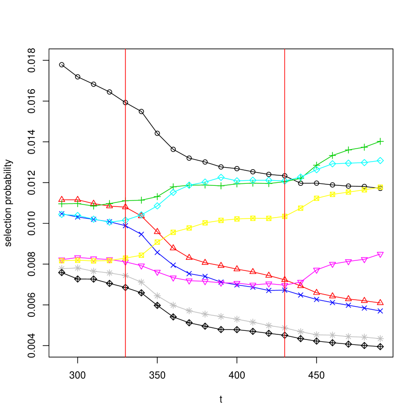
Figure 1: Impact of recommendation campaigns on the item probabilities: each curve displays the evolution of $P(i)$ over time for a given item.

The skill functionality has been implemented at time $t=0$. After 300 days, some of the $P_{t}(i)$ are roughly static. Probabilities of other items still evolve over time under various influences, but the major sources of evolution are recommendation campaigns. Indeed, at times $t=330$ and $t=430$, recommendation campaigns have been conducted: users have received personalized recommendation of skills to add to their profiles. The figure shows strong modifications of the $P_{t}(i)$ quickly after each campaign. In particular, the probabilities of the items which have been recommended increase significantly; this is the case for the black, pink and light blue curves at $t=330$. On the other hand, the probabilities of the items which have not been recommended decrease at the same time. The probabilities tend to become stable again until the same phenomenon can be observed right after the second recommendation campaign at $t=430$: the curves corresponding to the items that have been recommended again keep increasing. The green curve represents the probability of an item which has been recommended only during the second recommendation campaign. Section 4.2 demonstrates the effects of this evolution on algorithm evaluations.

3 Reducing the evaluation bias

3.1 Principle for reducing the bias

Let us consider a naive algorithm which always recommends the same items whatever the user and historical data. In other words, $g$ is constant. Constant algorithms are particularly easy to understand and useful to illustrate the bias due to external factors. Indeed one can reasonably assume that the score of such algorithms does not strongly vary over time.

A simple transformation of equation (1) shows that for a constant algorithm $g$:

$$L_{t}(g) =\sum_{u\in U}\sum_{i\in I}P_{t}(i|u)P_{t}(u)l(g_{t},i)$$

$$=\sum_{i\in I}l(g_{t},i)\sum_{u\in U}P_{t}(i|u)P_{t}(u)$$

$$=\sum_{i\in I}P_{t}(i)l(g_{t},i).$$ (2)

As a consequence, a way to guarantee a stationary evaluation framework for a constant algorithm is to have constant values for the $P_{t}(i)$ (the marginal distribution of the items).

A natural solution to have constant values for $P_{t}(i)$ would be to record those probabilities at $t_{0}$ and use them subsequently in offline evaluation as the probability to select an item. However, this would require to revert the way offline evaluation is done: first select an item, then select a user having this item with a certain probability $\pi_{t}(u|i)$. But as the probability law originally defined on users reflects their relative importance and should not be modified, it will be necessary to compute $\pi_{t}(u|i)$ such as the overall probability law on users is close enough to the original one $\big{(}P_{t_{0}}(u)\big{)}$. The computation of the coefficients $\pi_{t}(u|i)$ would need to be done for all users. Keeping the standard offline evaluation procedure and computing coefficients to alter the probabilities of selecting an item for a given user is more efficient because it can be done only for a limited number of key items (in practice in much smaller quantity than the number of users for most of real world systems) leading to a much lower complexity.

A strong assumption we make is that in practice reducing offline evaluation bias for constant algorithms contributes to reducing offline evaluation bias for all algorithms.

3.2 Item weights

$P_{t}(i|u)$ probabilities are thus the only quantities that can be modified in order to reduce the bias of offline evaluation. In particular, $P_{t}(u)$ is driven by business considerations related to the importance of individual users and can seldom be manipulated without impairing the associated business metrics. We propose therefore to depart from the classical values for $P_{t}(i|u)$ (such as using a uniform probability) in order to mimic static values for $P_{t_{0}}(i)$. This approach is related to the weighting strategy used in the case of covariate shift [sugiyama2007covariate].

This is implemented via tunable item specific weights, the $\omega=(\omega_{i})_{i\in I}$, which induce modified conditional probabilities $P_{t}(i|u,\omega)$. The general idea is to increase the probability of selecting $i$ if $\omega_{i}$ is larger than 1 and vice versa, so that $\omega$ recalibrates the probability of selecting each item. The simplest way to implement this probability modification is to define $P_{t}(i|u,\omega)$ as follows:

$$P_{t}(i|u,\omega)=\frac{\omega_{i}P_{t}(i|u)}{\sum_{j\in I_{t}}\omega_{j}P_{t}(j|u)}.$$ (3)

Other weighting schemes could be used. Notice that these weighted conditional probabilities lead to weighted item probabilities defined by:

$$P_{t}(i|\omega)=\sum_{u\in U}P_{t}(i|u,\omega)P_{t}(u).$$ (4)

3.3 Adjusting the weights

We thus reduce the evaluation bias by leveraging the weights $\omega$ and using the associated distribution $P_{t_{1}}(i|u,\omega)$ instead of $P_{t_{1}}(i|u)$. Indeed one can chose $\omega$ in such as way that $P_{t_{1}}(i|\omega)\simeq P_{t_{0}}(i)$. This allows one to use all the data available at time $t_{1}$ for the offline evaluation while limiting the bias induced by those new data.

This leads to a non-linear system with $n_{i}$ equations and $n_{i}$ parameters ($\omega_{1},\dots,\omega_{n_{i}}$) such that for all $i\in I_{t_{1}}$:

$$\sum_{u\in U}\frac{\omega_{i}P_{t_{1}}(i|u,\omega_{i})}{\sum_{j\in I}\omega_{j}P_{t_{1}}(j|u,\omega_{j})}\cdot P_{t_{1}}(u)=P_{t_{0}}(u)$$

$\omega$ cannot be solved easily and we thus need to approximate it using an optimisation algorithm.

Optimizing the weights amounts to reducing a dissimilarity between the weighted distribution and the original one. We use here the Kullback-Leibler divergence, that is

$$D(\omega) =D_{KL}(P_{t_{0}}(.)\|P_{t_{1}}(.|\omega))$$

$$=\sum_{i\in I_{t_{0}}}P_{t_{0}}(i)\log\frac{P_{t_{0}}(i)}{P_{t_{1}}(i|\omega)}.$$ (5)

Where $I_{t_{0}}$ represents the set of items which have been selected at least once at $t_{0}$.

The asymmetric nature of $D_{KL}$ is useful in our context as it reduces the influence of rare items at time $t_{0}$ as they were not very important in the calculation of $L_{t_{0}}(g)$.

The target probability $P_{t_{0}}(i)$ is computed once and for all items at the initial evaluation time. One coordinate of the gradient can be computed in $\mathcal{O}(N_{U\times I_{t_{1}}})$, where $N_{U\times I_{t_{1}}}$ is the number of couples $(u,i)$ with $i\in I_{u}$ and $u\in U$ at instant $t_{1}$. Thus the whole gradient can be computed in complexity $\mathcal{O}(n_{i}\cdot N_{U\times I_{t_{1}}})$. This would be prohibitive on a large system. To limit the optimization cost, we focus on the largest modifications between $P_{t_{0}}(i)$ and $P_{t_{1}}(i)$. More precisely, we compute once $P_{t_{1}}(i)$ for all $i\in I_{t_{0}}$ and select the subset $I_{t_{0}}^{t_{1}}(p)$ of $I_{t_{1}}$ of size $p$ which exhibits the largest differences in absolute values between $P_{t_{0}}(i)$ and $P_{t_{1}}(i)$.

Then $D(\omega)$ is only optimized with respect to the corresponding weights $(\omega_{i})_{i\in I_{t_{0}}^{t_{1}}(p)}$, leading to a cost in $\mathcal{O}(p\cdot N_{U\times I_{t_{1}}})$ for each gradient calculation. Notice that $p$ is therefore an important parameter of the weighting strategy. In practice, we optimize the divergence via a basic gradient descent.

Notice that to implement weight optimization, one needs to compute $P_{t_{0}}(i)$ and $P_{t_{1}}(i)$. As pointed out in 3.1 these are costly operations. We assume however that evaluating several recommendation algorithms has a much larger cost, because of the repeated evaluation of $L_{t}(g)$ associated to e.g. statistical model parameter tuning. Then while optimizing $\omega$ is costly, it allows one to rely on the efficient classical offline strategy to evaluate recommendation algorithms with a reduced bias.

4 Experimental evaluation

4.1 Data and metrics

The proposed approach is studied on real world data extracted from the Viadeo professional social network. The recommendation setting is the one described in Section 2.3: users can attach skills to their profile. Skills are recommended to the users in order to help them build more accurate and complete profiles. In this context, items are skills. The data set used for the analysis contains 34 448 users and 35 741 items. The average number of items per user is 5.33. The distribution of items per user follows roughly a power law, as shown on Figure 2.

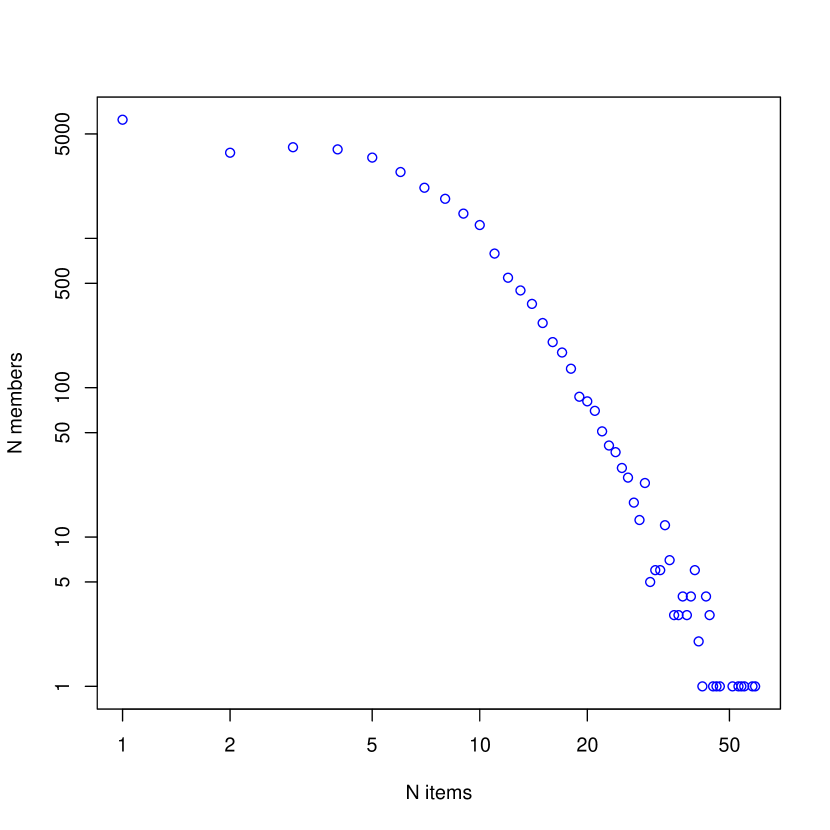
Figure 2: Distribution of items per user

Both probabilities $P_{t}(u)$ and $P_{t}(i|u)$ are uniform. The quality function $l$ is given by $l(g_{t}(u_{-i}),i)=\mathds{1}_{i\in g_{t}(u_{-i})}$ where $g_{t}(u_{-i})$ consists in 5 items. We use constant recommendation algorithms to focus on the direct effects of our weighting proposal, which means here that each algorithm is based on a selection of 5 items that will be recommended to all users.

The quality of a recommendation algorithm, $L_{t}(g)$, is estimated via stochastic sampling in order to simulate what could be done on a larger data set than the one used for testing. We selected repeatedly 20 000 users (uniformly among the 34 448, including possible repetitions) and then one item per user (according to $P_{t}(i|u)$ or $P_{t}(i|u,\omega)$).

The analysis is conducted on a 201 days period, from day 300 to day 500. Day 0 corresponds to the launch date of the skill functionality. As noted in Section 2.3 two recommendation campaigns were conducted by Viadeo during this period at $t=330$ and $t=430$ respectively.

4.2 Bias in action

We first demonstrate the effect of the bias on two constant recommendation algorithms. The first one $g^{1}$ is modeled after the actual recommendation algorithm used by Viadeo in the following sense: it recommends the five most recommended items from $t=320$ to $t=480$. The second algorithm $g^{2}$ takes the opposite approach by recommending the five most frequent items at time $t=300$ among the items that were never recommended from $t=320$ to $t=480$. In a sense, $g^{1}$ agrees with Viadeo’s recommendation algorithm, while $g^{2}$ disagrees.

Figure 3: Evolution of $L_{t}(g^{1})$ over time ($g^{1}$ “agrees” with the recommendation algorithm)

Figure 4: Evolution of $L_{t}(g^{2})$ over time ($g^{2}$ “disagrees” with the recommendation algorithm)

Figures 3 and 4 show the evolution of $L_{t}(g^{1})$ and $L_{t}(g^{2})$ over time. As both algorithms are constant, it would be reasonable to expect minimal variations of their offline evaluation scores. However in practice the estimated quality of $g^{1}$ increases by more than 25 %, while the relative decrease of $g^{2}$ reaches 33 %.

4.3 Reduction of the bias

We apply the strategy described in Section 3 to compute optimal weights at different instants and for several values of the $p$ parameter. Results are summarized in Figures 5 and 6.

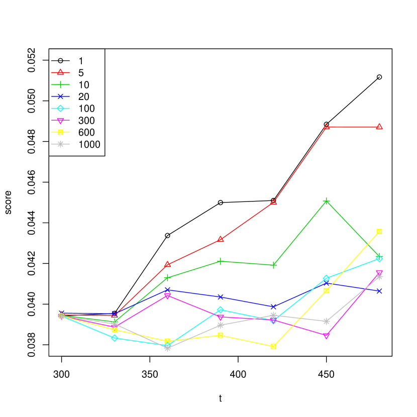
Figure 5: Evolution of $L_{t}(g^{1})$ over time ($g^{1}$ “agrees” with the recommendation algorithm) when items are weighted (see text for details).

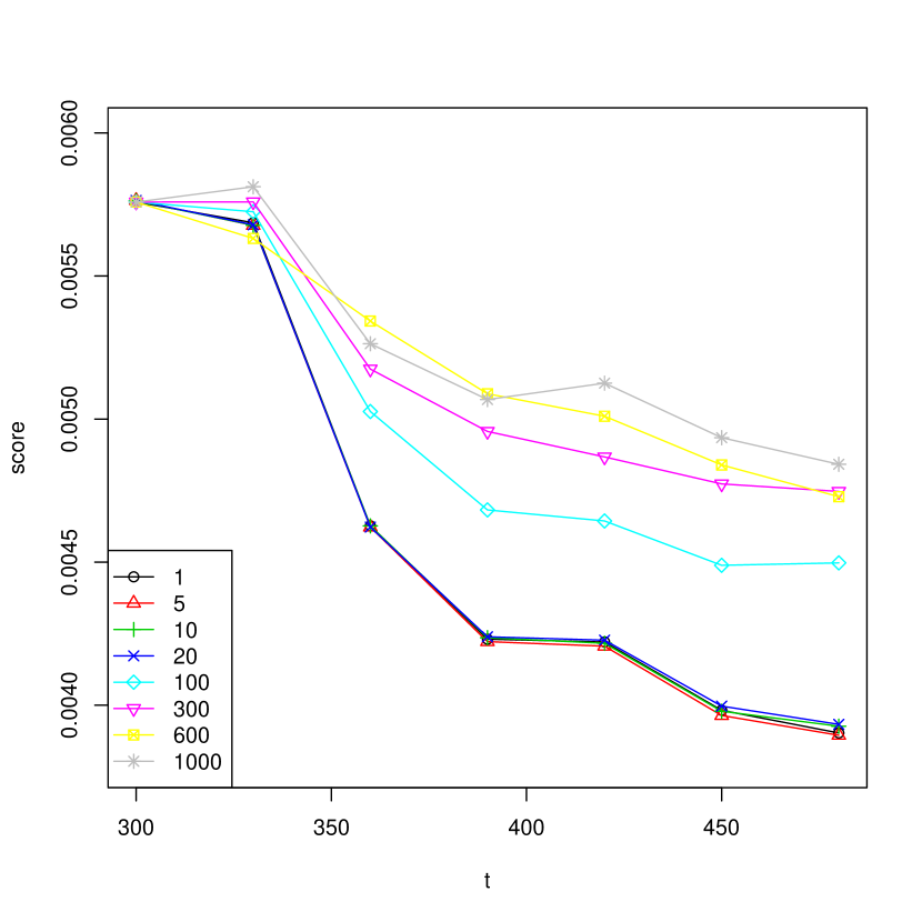
Figure 6: Evolution of $L_{t}(g^{2})$ over time ($g^{2}$ “disagrees” with the recommendation algorithm) when items are weighted (see text for details).

The figures show clearly the stabilizing effects of the weighting strategy on the scores of both algorithms. In the case of algorithm $g^{1}$, the stabilisation is quite satisfactory with only $p=20$ active weights. This is expected because $g^{1}$ agrees with Viadeo’s recommendation algorithm and therefore recommends items for which probabilities $P_{t}(i)$ change a lot over time. Those probabilities are exactly the ones that are corrected by the weighting technique.

The case of algorithm $g^{2}$ is less favorable, as no stabilisation occurs with $p\leq 20$. This can be explained by the relative stability over time of the probabilities of the items recommended by $g^{2}$ (indeed, those items are not recommended during the period under study). Then the perceived reduction in quality over time is a consequence of increased probabilities associated to other items. Because those items are never recommended by $g^{2}$, they correspond to direct recommendation failures. In order to stabilize $g^{2}$ evaluation, we need to take into account weaker modifications of probabilities, which can only be done by increasing $p$. This is clearly shown by Figure 6.

5 Conclusion

We have analyzed the offline evaluation bias induced by various factors that have influenced historical data as the recommendation algorithms previously used for such an online system. Indeed, as recommendations influence users, a recommendation algorithm in production tends to be favored by offline evaluation over time. On the contrary, an algorithm with different recommendations will generally witness over time a reduction of its offline evaluation score. To overcome this bias, we have introduced a simple item weighting strategy inspired by techniques designed for tackling the covariate shift problem. We have shown on real world data extracted from Viadeo professional social network that the proposed technique reduces the evaluation bias for constant recommendation algorithms.

While the proposed solution is very general, we have only focused on the simplest situation of constant recommendations evaluated with a binary quality metric (an item is either in the list of recommended items or not). Further works include the confirmation of bias reduction on more elaborate algorithms, possibly with more complex quality functions. The trade off between the computational cost of the proposed solution and its quality should also be investigated in more details.

Appendix A Algorithmic details

A.1 Gradient calculation

We optimize $D(\omega)$ with a gradient based algorithm and hence $\nabla D$ is needed. Let $i$ and $k$ be two distinct items $i\neq k$, then

$$\frac{\partial P(i|u,\omega)}{\partial\omega_{k}} =-\frac{\omega_{i}P(i|u)P(k|u)}{\left(\sum_{j\in I}\omega_{j}P(j|u)\right)^{2}},$$

$$=-P(i|u,\omega)\frac{P(k|u,\omega)}{\omega_{k}}.$$ (6)

We have also

$$\frac{\partial P(i|u,\omega)}{\partial\omega_{i}}=\frac{P(i|u,\omega)}{\omega_{i}}\left(1-P(i|u,\omega)\right),$$ (7)

and therefore for all $k$:

$$\frac{\partial P(i|u,\omega)}{\partial\omega_{k}}=\frac{P(k|u,\omega)}{\omega_{k}}\left(\delta_{ik}-P(i|u,\omega)\right).$$ (8)

We have implicitly assumed that the evaluation is based on independent draws, and therefore:

$$P(i,k|\omega)=\sum_{u}P(i|u,\omega)P(k|u,\omega)P(u).$$ (9)

Then

$$\frac{\partial D(\omega)}{\partial\omega_{k}}=\\ \sum_{i}\frac{P_{t_{0}}(i)}{\omega_{k}P_{t_{1}}(i|\omega)}\left(P_{t_{1}}(i,k|\omega)-\delta_{ik}P_{t_{1}}(k|\omega)\right).$$ (10)

Application: if $P(u)\sim\mathcal{U}(U)$ and $P(i|U)\sim\mathcal{U}(I_{u})$, then:

$$P(u) = \frac{1}{\#U}$$

$$P(i|u) = \frac{1}{\#I_{u}}\cdot\mathds{1}_{i\in I_{u}}$$

$$P(i|\omega) = \frac{1}{\#U}\cdot\sum_{u\in U_{i}}\frac{\omega_{i}}{\sum_{j\in I_{u}}\omega_{j}}$$

$$P(i,k|\omega) = \frac{1}{\#U}\cdot\sum_{u\in U_{i}\cap U_{k}}\frac{\omega_{i}\omega_{k}}{(\sum_{j\in I_{u}}\omega_{j})^{2}}$$

Complexity: Assuming we have a sparse matrix $A\in\mathcal{M}{n_{U},n_{I}}(\mathbb{R})$ such as $A_{u,i}=\mathds{1}_{u\in I_{u}}$, we suggest to precalculate $P_{t_{0}}(i)$ and then for each coordinate of the gradient and for each $i$:

• compute $P(i|\omega)=\sum_{u\in U_{i}}P(i|u,\omega)P(u)$ in $\mathcal{O}(\#U_{i})$

• compute $P(i,k|\omega)=\sum_{i\in U_{i}}P(i|u,\omega)P(k|u,\omega)P(u)$ in $\mathcal{O}(\#U_{i})$

Then each $\frac{\partial D(\omega)}{\partial\omega_{k}}$ consists in a sum of $I$ terms computed in $\mathcal{O}(1)$, so that we can compute each coordinate of the gradient is $\mathcal{O}(\sum_{i\in I}U_{i})=\mathcal{O}(|A|)$.

Thus, as $|A|=N_{U\times I}$ the complexity to compute $p$ coordinates of the gradient is $\mathcal{O}(p\cdot N_{U\times I})$.

References

- Adomavicius & Tuzhilin, 2005 Adomavicius and Tuzhilin][2005]adomavicius2005toward Adomavicius, G., & Tuzhilin, A. (2005). Toward the next generation of recommender systems: A survey of the state-of-the-art and possible extensions. Knowledge and Data Engineering, IEEE Transactions on, 17, 734–749.
- Herlocker et al., 2004 Herlocker et al.][2004]HerlockerEtAl2004Evaluating Herlocker, J. L., Konstan, J. A., Terveen, L. G., & Riedl, J. T. (2004). Evaluating collaborative filtering recommender systems. ACM Transactions on Information Systems, 22, 5–53.
- Kantor et al., 2011 Kantor et al.][2011]kantor2011recommender Kantor, P. B., Rokach, L., Ricci, F., & Shapira, B. (Eds.). (2011). Recommender systems handbook. Springer.
- McNee et al., 2006 McNee et al.][2006]mcnee2006being McNee, S. M., Riedl, J., & Konstan, J. A. (2006). Being accurate is not enough: how accuracy metrics have hurt recommender systems. CHI’06 extended abstracts on Human factors in computing systems (pp. 1097–1101).
- Park et al., 2012 Park et al.][2012]park2012literature Park, D. H., Kim, H. K., Choi, I. Y., & Kim, J. K. (2012). A literature review and classification of recommender systems research. Expert Systems with Applications, 39, 10059–10072.
- Said et al., 2013 Said et al.][2013]said2013user Said, A., Fields, B., Jain, B. J., & Albayrak, S. (2013). User-centric evaluation of a k-furthest neighbor collaborative filtering recommender algorithm. Proceedings of the 2013 conference on Computer supported cooperative work (pp. 1399–1408).
- Shani & Gunawardana, 2011 Shani and Gunawardana][2011]shani2011evaluating Shani, G., & Gunawardana, A. (2011). Evaluating recommendation systems. In P. B. Kantor, L. Rokach, F. Ricci and B. Shapira (Eds.), Recommender systems handbook, 257–297. Springer.
- Shimodaira, 2000 Shimodaira][2000]Shimodaira2000227 Shimodaira, H. (2000). Improving predictive inference under covariate shift by weighting the log-likelihood function. Journal of Statistical Planning and Inference, 90, 227 – 244.
- Sugiyama et al., 2007 Sugiyama et al.][2007]sugiyama2007covariate Sugiyama, M., Krauledat, M., & Müller, K.-R. (2007). Covariate shift adaptation by importance weighted cross validation. The Journal of Machine Learning Research, 8, 985–1005.