Anomalous Diffusion of Self-Propelled Particles in Directed Random Environments

Abstract

We theoretically study the transport properties of self-propelled particles on complex structures, such as motor proteins on filament networks. A general master equation formalism is developed to investigate the persistent motion of individual random walkers, which enables us to identify the contributions of key parameters: the motor processivity, and the anisotropy and heterogeneity of the underlying network. We prove the existence of different dynamical regimes of anomalous motion, and that the crossover times between these regimes as well as the asymptotic diffusion coefficient can be increased by several orders of magnitude within biologically relevant control parameter ranges. In terms of motion in continuous space, the interplay between stepping strategy and persistency of the walker is established as a source of anomalous diffusion at short and intermediate time scales.

Anomalous transport of self-propelled particles in biological environments has received much recent attention Reviews . Of particular interest is the active motion of motor proteins along cytoskeletal filaments, which makes long-distance intracellular transport feasible Ross08 . The structural asymmetry of filaments results in a directed motion of motors with an effective processivity, denoting the tendency to move along the same filament. The processivity depends on the type of motor and filament ProcesivityRefs1 and it is strongly influenced by the presence of specific proteins or binding domains Vershinin07 ; ProcesivityRefs2 . In the limit of small unbinding rates it has been shown Klumpp05 that a walker on simple lattice structures moves superdiffusively at short time scales followed by a normal diffusion at long times. Similar results were reported for single bead motion on radially-organized microtubule networks Caspi00 . However, for general polarized cytoskeletal networks, the influence of structural complexity and motor processivity on the transport properties is not yet well understood. In this Rapid Communication, we introduce a coarse-grained perspective to the problem and show that the interplay between anisotropy and heterogeneity of the network and processivity leads to a rich transport phase diagram at short and intermediate time scales. The crossover times between different regimes and the asymptotic diffusion constant can vary by orders of magnitude when tuning the key parameters.

More precisely, a general analytical framework is developed to study persistent walks with arbitrary step-length and turning-angle distributions. We obtain an exact analytical expression for the dynamical evolution of the mean square displacement (MSD), displaying anomalous diffusion on varying time scales. The results can be also interpreted within the context of random motion in continuous space, e.g. in crowded biological media where the origin of subdiffusive motion is highly debated Subdiffusion3 ; Neusius09 ; CTRWFBM ; Jeon12b ; Bronstein09 ; Thiel13 .

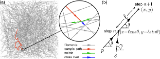
Figure 1: (color online) (a) A typical sample trajectory (red lines) on a random filamentous structure. Inset: Possible choices at the nodes of the directed network. (b) Path of the walker during two consecutive steps, described by Eq. (1).

While subdiffusion in cytoplasm slows down the transfer of matter, it is beneficial for a variety of cellular functions Sereshki12-Guigas08 ; Golding06 ; Weigel11 , since they depend on the localization of the involved reactants. The appearance of subdiffusion has been traced back to the presence of particular elements e.g. viscoelasticity or traps in the environment, and the resulting motion is commonly characterized by comparing it to different mathematical models, e.g., fractional Brownian motion FBM which is a mean-zero Gaussian process with long-ranged (anti-)correlation of displacements, or continuous time random walk CTRW which assumes a finite variance of step lengths and a heavy tailed distribution of waiting times, as experienced e.g. by tracer particles in entangled actin filament networks Wong04 or among random energy traps Burov07 . More recent studies even suggest the coexistence of both scenarios CTRWFBM ; Weigel11 . Here we verify that even in the absence of traps, viscoelasticity, overcrowding, etc., in the nature of the environment, the particle may still experience an anomalous motion within experimentally relevant time scales due to its stepping strategy. A specific strategy manifests itself for instance by the density, strength, and spatial obstacle arrangement and/or by external drives. We clarify the role of the variance of step lengths, the correlation between consecutive switching angles, and the persistency of the walker in displaying various types of motion.

Model and analytical solution.— We focus on the network interpretation in the following, and consider the motion of a walker on a randomly cross-linked network of polarized filaments [Fig. 1(a)]. The structural properties are characterized by probability distributions $R(\phi)$ for the angles $\phi$ between intersecting filaments, and $\mathcal{F}(\ell)$ for the segment lengths $\ell$ between neighboring intersections remark1 . Here we study a 2D network (extension to 3D is straightforward Shaebani13 ), and describe the motion of the particle by a Markovian process in discrete time and denote the probability density to be at position $(x,y)$ with a direction $\theta$ at time step $n$ by $P_{n}(x,y|\theta)$, whose dynamical evolution is defined by the master equation

$$\begin{aligned} &P\!\!_{{}_{n+1}}\!(x,y|\theta)=p\!\!\int\!\!\!d\ell\,\mathcal{F}(\ell)\,P\!\!_{{}_{n}}\!\big{(}x{-}\ell\text{cos}(\theta),y{-}\ell\text{sin}(\theta)\big{|}\theta\big{)}\\ &{+}s\!\!\int\!\!\!d\ell\,\mathcal{F}(\ell)\!\!\int_{-\pi}^{\pi}\!\!\!\!\!d\gamma\,R(\theta{-}\gamma)\,P\!\!_{{}_{n}}\!\big{(}x{-}\ell\text{cos}(\theta),y{-}\ell\text{sin}(\theta)\big{|}\gamma\big{)}.\end{aligned}$$ (1)

The probability of motion without changing the direction, $p$, represents the processivity of the motor, while $s{=}1{-}p$ describes a directional change [see Fig. 1(b)]. While it is quite difficult to obtain an explicit analytical expression for $P_{n}(x,y|\theta)$ from Eq. (1), it is possible to evaluate the moments of the displacement using an analytical Fourier–Z-transform technique Shaebani13 ; Sadjadi08 . We obtain the following exact expression for the MSD remark2

$$\frac{\langle r^{2}\rangle\!_{{}_{n}}}{\langle\ell\rangle^{2}}=\lambda\,n{+}\!\!\!\!\!\sum_{m{=}\pm 1}\!\!\!\frac{p{+}\mathcal{R}\!_{{}_{m}}{-}p\mathcal{R}\!_{{}_{m}}}{(1{-}p)(1{-}\mathcal{R}\!_{{}_{m}})}\bigg{[}n{+}\frac{(p{+}\mathcal{R}\!_{{}_{m}}{-}p\mathcal{R}\!_{{}_{m}})^{n}{-}1}{(1{-}p)(1{-}\mathcal{R}\!_{{}_{m}})}\bigg{]},$$ (2)

where $\mathcal{R}\!_{{}_{m}}$ is the Fourier transform of the intersection angle distribution, $\mathcal{R}\!_{{}_{m}}{=}\int_{-\pi}^{\pi}\text{d}\phi\;e^{\text{im}\phi}R(\phi)$, and $\lambda{=}\langle\ell^{2}\rangle/\langle\ell\rangle^{2}$ is the relative variance of $\mathcal{F}(\ell)$ which quantifies the heterogeneity of the network [Fig. 2(a)]. $\mathcal{R}\!_{{}_{m}}{\in}[-1,1]$ quantifies the correlation between the arrival direction before a switch and the final direction after it, thus, representing the anisotropy of the network. $\mathcal{R}\!_{{}_{m}}{=}0$ corresponds to the uniform case, and negative (positive) values of $\mathcal{R}\!_{{}_{m}}$ to an increased probability for motion in the near backward (forward) directions [Fig. 2(b)]. Although our method allows us to handle an arbitrary function $R(\phi)$, here we consider only symmetric distributions with respect to the arrival direction ($\mathcal{R}\!_{{}_{-1}}{=}\mathcal{R}\!_{{}_{+1}}{\equiv}\mathcal{R}$), as it is usually the case in biological applications. The results remain valid in three dimensions for a cylindrical symmetry of $R(\phi)$. In the simple case of walking with left-right symmetry and without persistency, Eq. (2) reduces e.g. to a model for cell migration along surfaces Nossal74 .

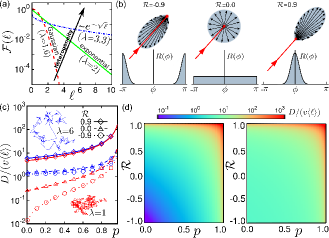
Figure 2: (color online). (a) Evolution of $\lambda$ with $\mathcal{F}(\ell)$. (b) Examples of $R(\phi)$ and their corresponding anisotropy parameter $\mathcal{R}$. Insets: Black arrows show the possible directions of motion at the next step, with length being proportional to the probability. (c) Asymptotic diffusion coefficient vs $p$ at different $\mathcal{R}$, from simulations (symbols) and analytical predictions via Eq. (3) (curves). The red (blue) color corresponds to $\lambda=1\,(6)$. Insets: Typical trajectories at $p{=}\mathcal{R}{=}0$. (d) 2D profiles of $D$ in $p{-}\mathcal{R}$ plane for $\lambda{=}1$ (left) and $\lambda{=}6$ (right).

Asymptotic behavior.— In the limit of $n{\rightarrow}\infty$ the terms with $(p{+}\mathcal{R}{-}p\mathcal{R})^{n}$ in Eq. (2) vanish since $|p{+}\mathcal{R}{-}p\mathcal{R}|{\leq}1$. Hence the linear term dominates and the motility becomes purely diffusive. The asymptotic diffusion constant is given by

$$D=\frac{1}{4}v\langle\ell\rangle\bigg{[}\lambda+\frac{2(p{+}\mathcal{R}{-}p\mathcal{R})}{(1{-}p)(1{-}\mathcal{R})}\bigg{]},$$ (3)

with $v$ being the average motor velocity. Figures 2(c),(d) show that $D$ varies by several orders of magnitude by varying the anisotropy and heterogeneity measures, $\mathcal{R}$ and $\lambda$, and the processivity $p$. The results of extensive Monte Carlo simulations for persistent walk on structures obtained from the same $R(\phi)$ and $\mathcal{F}(\ell)$ distributions agree perfectly with analytical predictions. The linearly additive contribution of $\lambda$ in Eq. (3) is negligible when $p,\mathcal{R}{\rightarrow}1$ but dominates for $p,\mathcal{R}{\ll}1$ and large $\lambda$. Intuitively, a broader distribution $\mathcal{F}(\ell)$ corresponds to a larger asymptotic diffusion coefficient $D$ (e.g. $D_{\text{exp}}/D_{\text{Gaussian}}{\simeq}1.27$ for $p{=}\mathcal{R}{=}0$). For a walker on square lattice with $p{=}0$, Eq. (3) reduces to $D{=}\frac{1}{4}v\langle\ell\rangle$ Klumpp05 . The negative values of $\mathcal{R}$ represent anticorrelation between consecutive switching angles. A pure localization ($D{=}0$) happens when $\mathcal{R}{=}-1$, $p{=}0$, and $\lambda{=}1$.

Motor proteins are highly flexible to turn even up to $150^{\circ}$ at intersections ProcesivityRefs1 , and have a typical velocity $v{\sim}1\mu\text{m/s}$ Ali08 . $\mathcal{R}$ may vary from $0$ for a random actin-filament structure to $1$ for radially-organized microtubule networks, and processivity can be tuned at least within the range $0.1{-}0.7$ ProcesivityRefs2 ; Vershinin07 . Hence, for an actin network with an average mesh size $\langle\ell\rangle{\sim}100\,\text{nm}$ Wong04 , $D$ may vary by $3$ orders of magnitude from $10^{-2}$ to $10\mu\text{m}^{2}\text{/s}$.

Different regimes of motion.— A random walker with a constant step length and uniform rotation angle ($p{=}\mathcal{R}{=}0$) conceivably displays normal diffusion at all time scales. In the general case, however, we predict a rich variety of the MSD profiles, as shown in Fig. 3. The profile shapes strongly depend on the choice of $\lambda$, $p$, and $\mathcal{R}$. An oscillatory dynamics emerges at large negative values of $\mathcal{R}$, where the motion is strongly antipersistent and the particle hops frequently back and forth without a significant net motion. Such behavior is observed for the antipersistent motion of paramagnetic colloids in a periodically switching magnetic potential Tierno12 .

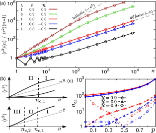
Figure 3: (color online). (a) MSD vs $n$ at different $\lambda$, $p$, and $\mathcal{R}$, from simulations (symbols) and theory via Eq. (2) (curves). (b) Schematic representation of the possible regimes of motion and the crossover times. (c) The crossover time $n_{\text{c,1}}$ vs $p$ for different values of $\mathcal{R}$, for $\lambda{=}1$ (red) and $\lambda{=}6$ (blue).

Although the asymptotic dynamics of a system described by Eq. (2) is diffusive, the corresponding diffusion scaling $\langle\textbf{r}^{2}\rangle{\propto}Dn$ might be observable only on time- and length scales which are experimentally not accessible. We denote the asymptotic regime by I and the preceding regime (oscillatory, sub- or super-diffusive) by II [Fig. 3(b)]. The smooth crossover from regime II to I occurs at a characteristic time scale $n_{\text{c},1}$ which strongly varies with the parameter values [see Fig. 3(a)]. $n_{\text{c},1}$ is identified by balancing the term linear in $n$ in Eq. (2) and the non-linear contribution. Figure 3(c) shows that $n_{\text{c},1}$ varies over several orders of magnitude. For an actin network, the time scale for motors to travel between filament junctions is ${\sim}0.1\,\text{sec}$ (see above), and thus $n_{\text{c},1}$ ranges from less than $10^{-1}$ up to more than $10^{2}$ seconds for the motion of motor proteins on actin filament networks. Experimentally, it is often difficult to perform measurements in a time window which is wide enough to ensure that all different regimes of motion are realized.

$n_{\text{c},1}$ decreases with increasing $\lambda$, i.e. heterogeneity extends the diffusive regime I to smaller times. While $n_{\text{c},1}$ increases monotonically with $p$ for $\mathcal{R}{\geq}0$, it exhibits a nonmonotonic dependence for $\mathcal{R}{<}0$, with the minimum value $n_{\text{c},1}{=}1$ at a processivity $p\!_{{}_{\text{min}}}{\simeq}\mathcal{R}/(\mathcal{R}{-}1)$. When $\mathcal{R}{>}0$, $p$ and $\mathcal{R}$ cooperate in enhancing net forward motion which results in a superdiffusive dynamics in regime II. Therefore, increasing $p$ while $\mathcal{R}{\geq}0$ leads to stronger superdiffusion and postpones the transition to regime I, reflected by a monotonic increase of $n_{\text{c},1}$. In contrast, $p$ and $\mathcal{R}$ compete when $\mathcal{R}{<}0$, which may lead to a variety of anomalous diffusion scenarios, depending on their relative importance. With increasing $p$ from zero at a negative $\mathcal{R}$, the anticorrelation of rotation angles initially dominates the dynamics and causes oscillations or subdiffusion. However, the role of processivity $p$ becomes gradually more pronounced and a transition from sub to superdiffusion happens in regime II at the turning point $p\!_{{}_{\text{min}}}$. Thus the varying strength and type of anomaly are the reasons behind the nonmonotonic behavior of $n_{\text{c},1}$.

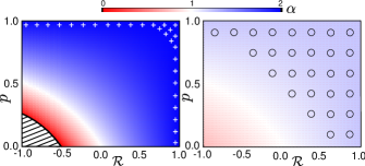
Figure 4: (color online). 2D profiles of the phase diagram of short time dynamics in the $p{-}\mathcal{R}$ plane for $\lambda{=}1$ (left) and $\lambda{=}6$ (right). The color intensity reflects the magnitude of anomalous exponent $\alpha$, with red (blue) meaning sub- (super-) diffusion. The white plus symbols and hatched lines denote the ballistic and oscillatory subdomains. The circles mark the regions of the $p{-}\mathcal{R}$ parameter space where the slope of $\langle\textbf{r}^{2}\rangle$ initially grows with time (regime III). The blue-red (red-oscillatory) interface is specified by $p{=}\frac{\mathcal{R}}{\mathcal{R}{-}1}$ ($p{+}\mathcal{R}{-}p\mathcal{R}{=}-\lambda{/}2$).

Short-time dynamics.— We determine an effective anomalous exponent $\alpha{=}1{+}\ln(1{+}\frac{p{+}\mathcal{R}{-}p\mathcal{R}}{\lambda})/\ln 2$ by fitting the initial $t$-dependence of the MSD to a power-law $\langle\textbf{r}^{2}\rangle{\sim}t^{\alpha}$. Fig. 4 summarizes the results of the anomalous short-term motion in a phase diagram in the ($p$,$\mathcal{R}$) space. The larger values of $\lambda$ imply effective exponents that are closer to $1$ as a consequence of the increasing role of the linear terms in $\langle\textbf{r}^{2}\rangle$. Above the threshold heterogeneity $\lambda_{c}{=}2$, the oscillatory phase no longer exists.

Finally, a closer look at $\langle\textbf{r}^{2}\rangle$ profiles reveals that in some of the superdiffusive cases the initial growth of $\langle\textbf{r}^{2}\rangle$ gets accelerated [regime III in Fig. 3(b)], although the curvature changes sign later, i.e. a crossover to regime II eventually happens. To explain this, we expand $\langle\textbf{r}^{2}\rangle$ around $n{=}1$ for the parameter values corresponding to the blue regions in Fig. 4, and find that the main contributions originate from the first and second order terms in $n$. From the competition between these terms we determine a characteristic (short) time scale $n_{\text{c},2}(\lambda,\mathcal{R},p){\simeq}2\big{[}(\lambda{+}\mathcal{A})(1{-}p)(1{-}\mathcal{R}){+}\mathcal{A}\;\text{ln}\mathcal{B}\big{]}/\big{[}\mathcal{A}\;(\text{ln}\mathcal{B})^{2}\big{]},$ where $\mathcal{B}{=}p{+}\mathcal{R}{-}p\mathcal{R}$ and $\mathcal{A}{=}2\mathcal{B}/[(1{-}p)(1{-}\mathcal{R})]$. At times $n{\ll}n_{\text{c},2}$, the linear term (${\sim}n$) plays the dominant role, thus, keeping the initial slope slightly above $1$ (regime III), while at $n_{\text{c},2}{\ll}n$ the second order term (${\sim}n^{2}$) dominates and the slope increases. By varying the control parameters, $n_{\text{c},2}$ can be pushed towards or away from $n{=}1$. In the limit of $n_{\text{c},2}{\rightarrow}1$, regime III disappears and the slope of $\langle\textbf{r}^{2}\rangle$ initially starts with the extremum value (regime II) and ends up with $1$. In the case that $1{\ll}n_{\text{c},2}$, all regimes exist. It turns out that the crossover time remains around $n_{\text{c},2}{\simeq}1$ for $\lambda{=}1$, i.e. regime III does not exist. However, with increasing $\lambda$, this regime appears for large values of $p$ and $\mathcal{R}$, and gradually spans the whole superdiffusive (blue) subdomain for large values of $\lambda$.

Comparison with experimental data.— Besides living organisms, the twofold interpretation of our methodology extends the applicability range of the results to the motion of self-propelled particles in continuous space in other realizations such as driven granular systems GranularRefs where the stepping properties of particles can be tuned by means of an external drive source and internal conditions remark1 . To validate the theoretical predictions, here we compare the analytical results with experiments in a nonliving system Tierno12 , where the accelerated motion of a paramagnetic tracer particle on a ferrite garnet film is controlled externally. The film displays a 2D array of magnetic bubbles with out-of-plane magnetization $M$, sitting on a hexagonal lattice of constant $L{=}11.6\mu\text{m}$. An external magnetic field switches between $\pm{H}$ with frequency $\omega$, which induces a certain degree of disorder in the shape and arrangement of the magnetic bubbles Soba08 . The resulting dynamic disorder (i.e. not reproducible after each cycle) influences the antipersistent motion of the tracer particle. In the absence of additional sources of anomalous behavior, such a labyrinthine environment provides an opportunity to examine the isolated impact of stepping strategy, which is tuned via remote control. For comparison, we also carried out simulations of motion on a dynamic disordered hexagonal lattice of synchronous flashing magnetic poles, which would closely mimic the experiment Shaebani13 . At each time step $\Delta t{=}\pi{/}\omega$, the new position of each node is randomly chosen within a circle of radius $L{\cdot}\delta$ around the corresponding node of the ordered hexagonal lattice ($\delta$ reflects the amount of disorder). The resulting step-length distribution $\mathcal{F}(\ell)$ of the tracer particle is fitted by a Gaussian centered at the size of the Wigner-Seitz cell, $L{/}2$, with a standard deviation e.g. $\sigma{\simeq}0.05L$ for $\delta{=}10\%$. With increasing $\delta$, the rotation-angle distribution $R(\phi)$ evolves from a single-peaked function at $\phi{=}\pi$ towards multiple peaks at $\phi{=}\pi,{\pm}2\pi{/}3,{\pm}\pi{/}3$. By tuning $\mathcal{R}$ in theory or the lattice disorder $\delta$ in simulations, the comparison with experimental data shows a remarkable agreement, as shown in Fig. 5. Notably, the frequency of oscillations is correctly reproduced and, moreover, one can derive the step-step correlations as $C_{s}(t){=}\mathcal{R}^{t\omega{/}\pi}$, which gives rise to the same behavior reported in Tierno12 .

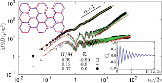
Figure 5: (color online). MSD versus time for a paramagnetic tracer particle in the two-state flashing potential. The analytical (solid lines) and simulation (dashed lines) fits are compared with experimental data (symbols) taken from Fig. 2 of Tierno12 . Insets: (top) Schematic picture of two consecutive disordered lattices in simulations with $\delta{=}10\%$. (bottom) The normalized step-step correlation function $C_{s}$ vs. time.

Discussion.— To establish the interplay between processivity and structural properties of cytoskeleton as a source of anomalous motion, we have taken only angular correlations into account in the present model, which defines a characteristic correlation scale beyond which the motion is diffusive (see the inset of Fig. 5). However, the formalism can be generalized in different ways, e.g. by introducing a long-range (anti-)cross-correlation between the angular and step-length distributions, leading to a stationary increment as observed in viscous environments. Moreover, intermittent walks can be considered, using a set of coupled master equations. By handling different modes of motility (e.g. binding and unbinding of motor proteins, or a combined waiting-running motion as experienced in the presence of traps or in overcrowded environments), one can obtain exact expressions for the time evolution of arbitrary moments of displacement. The possibility of handling arbitrary stepping roles in our approach, which is not feasibly available in other approaches, provides a unique opportunity to study more complex situations and develop models with predictive power.

We verified that self-propelled particles display a wide range of different types of motion on complex structures. We disentangled the combined effects of processivity and structural properties of the underlying network on transport properties. The method relates the microscopic details of the transport network or the characteristics of the particle dynamics to macroscopically observable transport coefficients such as the diffusion coefficient, without using phenomenological or purely mathematical models. The results point to new strategies to unravel the structural complexity of filamentous networks or non-biological realizations such as porous media by monitoring the motion of tracer particles which perform a random walk on such environments.

We thank P. Tierno for supplying the experimental data. This work was supported by DFG within SFB 1027 (projects A7, A3), and BMBF (FKZ 03X0100C).

References

- (1) P. C. Bressloff and J. M. Newby, Rev. Mod. Phys. 85, 135 (2013); F. Höfling and T. Franosch, Rep. Prog. Phys. 76, 046602 (2013).
- (2) J. L. Ross, M. Y. Ali, and D. M. Warshaw, Curr. Opin. Cell Biol. 20, 41 (2008).
- (3) M. Y. Ali et al., Proc. Natl. Acad. Sci. 104, 4332 (2007); K. Shiroguchi and K. Kinosita, Science 316, 1208 (2007).
- (4) M. Vershinin et al., Proc. Natl. Acad. Sci. 104, 87 (2007).
- (5) Y. Okada, H. Higuchi, and N. Hirokawa, Nature 424, 574 (2003); T. L. Culver-Hanlon et al., Nat. Cell Biol. 8, 264 (2006).
- (6) S. Klumpp and R. Lipowsky, Phys. Rev. Lett. 95, 268102 (2005).
- (7) A. Caspi, R. Granek, and M. Elbaum, Phys. Rev. Lett. 85, 5655 (2000).
- (8) S. M. A. Tabei et al., Proc. Natl. Acad. Sci. 110, 4911 (2013); S. C. Weber, A. J. Spakowitz, and J. A. Theriot, Phys. Rev. Lett. 104, 238102 (2010).
- (9) T. Neusius, I. M. Sokolov, and J. C. Smith, Phys. Rev. E 80, 011109 (2009).
- (10) J.-H. Jeon, H. M.-S. Monne, M. Javanainen, and R. Metzler, Phys. Rev. Lett. 109, 188103 (2012).
- (11) I. Bronstein et al., Phys. Rev. Lett. 103, 018102 (2009).
- (12) B. Wang, J. Kuo, S. Ch. Bae, and S. Granick, Nat. Mater. 11, 481 (2012); M. Magdziarz, A. Weron, K. Burnecki, and J. Klafter, Phys. Rev. Lett. 103, 180602 (2009).
- (13) F. Thiel, F. Flegel, and I. M. Sokolov, Phys. Rev. Lett. 111, 010601 (2013).
- (14) I. Golding and E. C. Cox, Phys. Rev. Lett. 96, 098102 (2006).
- (15) L. E. Sereshki, M. A. Lomholt, and R. Metzler, Europhys. Lett. 97, 20008 (2012); G. Guigas and M. Weiss, Biophys. J. 94, 90 (2008).
- (16) A. V. Weigel, B. Simon, M. M. Tamkun, and D. Krapf, Proc. Natl. Acad. Sci. 108, 6438 (2011).
- (17) B. B. Mandelbrot and J. W. Van Ness, SIAM Rev. 10, 422 (1968); E. Lutz, Phys. Rev. E 64, 051106 (2001).
- (18) B. D. Hughes, Random Walks and Random Environments, Vol. 1 (Clarendon Press, Oxford, 1995); R. Metzler and J. Klafter, Phys. Rep. 339, 1 (2000).
- (19) I. Y. Wong et al., Phys. Rev. Lett. 92, 178101 (2004).
- (20) S. Burov and E. Barkai, Phys. Rev. Lett. 98, 250601 (2007).
- (21) and can be interpreted as rotation-angle and step-length probabilities in the continuous space.
- (22) M. R. Shaebani, Z. Sadjadi, H. Rieger, and L. Santen, in preparation (2014).
- (23) Z. Sadjadi, M.-F. Miri, M. R. Shaebani, and S. Nakhaee, Phys. Rev. E 78, 031121 (2008).
- (24) This particular result can also be obtained by adapting other analytical techniques (see e.g. Nossal74 ; Kareiva83 ), yet, our method is directly applicable to a large class of persistent random walk problems, which are out of scope for the other methods.
- (25) R. Nossal and G. H. Weiss, J. Theor. Biol. 47, 103 (1974).
- (26) P. M. Kareiva and N. Shigesada, Oecologia 56, 234 (1983).
- (27) M. Y. Ali, H. Lu, C. S. Bookwalter, D. M. Warshaw, and K. M. Trybus, Proc. Natl. Acad. Sci. 105, 4691 (2008).
- (28) P. Tierno, F. Sagués, T. H. Johansen, and I. M. Sokolov, Phys. Rev. Lett. 109, 070601 (2012).
- (29) A. Kudrolli, G. Lumay, D. Volfson, and L. S. Tsimring, Phys. Rev. Lett. 100, 058001 (2008); M. R. Shaebani, J. Sarabadani, and D. E. Wolf, Phys. Rev. Lett. 108, 198001 (2012).
- (30) A. Soba, P. Tierno, T. M. Fischer, and F. Sagués, Phys. Rev. E 77, 060401(R) (2008).