Asymptotic stability of solitary waves in generalized Gross–Neveu model

Abstract

For the nonlinear Dirac equation in (1+1)D with scalar self-interaction (Gross–Neveu model), with quintic and higher order nonlinearities (and within certain range of the parameters), we prove that solitary wave solutions are asymptotically stable in the “even” subspace of perturbations (to ignore translations and eigenvalues $\pm 2\omega i$). The asymptotic stability is proved for initial data in $H^{1}$. The approach is based on the spectral information about the linearization at solitary waves which we justify by numerical simulations. For the proof, we develop the spectral theory for the linearized operators and obtain appropriate estimates in mixed Lebesgue spaces, with and without weights.

1 Introduction

Models of self-interacting spinor fields have been appearing in particle physics for many years [Iva38, FLR51, FFK56, Hei57]. The most common examples of nonlinear Dirac equation are the massive Thirring model [Thi58] (vector self-interaction) and the Soler model [Sol70] (scalar self-interaction). The (1+1)D analogue of the latter model is widely known as the massive Gross–Neveu model [LG75]. In the present paper, we address the asymptotic stability of solitary waves in this model. We require that the nonlinearity in the equation vanishes of order at least five; the common case of cubic nonlinearity seems out of reach with the current technology; there is a similar situation with other popular dispersive models in one spatial dimension, such as the Schrödinger and Klein-Gordon equations (see [BP92a, BP92b, Miz08, Cuc08, KNS12] and the references therein).

We only consider perturbations in the class of “even” spinors (same parity as the solitary waves under consideration). The restriction to this subspace allows us to ignore spatial translations and the $\pm 2\omega i$ eigenvalues which are present in the spectrum of the linearization at solitary waves [Com11]. This paper therefore may be considered as the extension of [PS12] to the translation-invariant systems (in that paper, the potential was needed to obtain the desired spectrum of linearization at small amplitude solitary waves).

A similar result – asymptotic stability of solitary waves in the translation-invariant nonlinear Dirac equation in three spatial dimensions – is obtained in [BC12c]. Authors base their highly technical approach on a series of assumptions about the spectrum of the linearizations at solitary waves; these assumptions can not be verified yet for a particular model. The authors also restrict the perturbations to a certain subspace to avoid spatial translations and issues caused by the presence of $\pm 2\omega i$ eigenvalues [Com11] and only consider the solitary waves with $\omega>m/3$. Contrary to [BC12c], our results are obtained for models for which the spectrum is known (albeit numerically); our technical restriction is $\lvert\omega\rvert<m/3$.

We briefly review the related research on stability of solitary waves in nonlinear Dirac equation. There have been numerous approaches to this question based on considering the energy minimization at particular families of perturbations, but the scientific relevance of these conclusions has never been justified; see the review and references in e.g. [BC12b, SQM⁺14]. The linear (spectral) stability of the nonlinear Dirac equation is still being settled. According to [BC12b], the linear stability properties of solitary waves in the nonrelativistic limit of the nonlinear Dirac equation (solitary waves with $\omega\lesssim m$) are similar to linear stability of nonlinear Schrödinger equation; in particular, the stability of the ground states (no-node solutions) is described by the Vakhitov–Kolokolov stability criterion [VK73], $\partial_{\omega}Q(\omega)<0$, with $Q(\omega)=\left\|\phi_{\omega}\right\|_{L^{2}}^{2}$ the charge of a solitary wave. Away from the nonrelativistic limit, the border of the instability region can be indicated by the conditions $\partial_{\omega}Q(\omega)=0$ or $E(\omega)=0$ (the value of the energy functional at a solitary wave), see [CBS13]. The instability could also develop from the bifurcation of the quadruple of complex eigenvalues from the embedded thresholds $\pm i(m+\lvert\omega\rvert)$ as in [BPZ98], which in particular can take place at the collision of thresholds at $\lambda=\pm im$ when $\omega=0$ as in [KS02]. We do not have a good criterion when such bifurcation takes place.

Let us mention that our results are at odds with the numerical simulations in [SQM⁺14] which are interpreted as instability of the cubic Gross–Neveu model ($k=1$) for $\omega\leq\omega_{c}\approx 0.56$, of the quintic model ($k=2$) for $\omega\leq\omega_{c}\approx 0.92$, and of the $k=3$ model for all $\omega<m$. We expect that the observed instability is related to the boundary effects, when certain harmonics, instead of being dispersed, are reflected into the bulk of the solution, where the nonlinearity creates higher harmonics; this process keeps repeating, and eventually the space-time discretization becomes insufficient. This explanation is corroborated by the fact that the characteristic instability times grow almost proportionally with the size of the domain (see the instability times for the one-humped solitary wave with $k=1$, $\omega=0.5$ in [SQM⁺14, TABLE II]), suggesting the link not to the linear instability but to the boundary contribution. Our numerics show no complex eigenvalues away from the union of real and imaginary axes in the Gross–Neveu model with $1\leq k\leq 9$. The presence of real eigenvalues (as on Figure 2) agrees with the Vakhitov–Kolokolov stability criterion, $dQ(\omega)/d\omega>0$.

The approach in our paper is standard, being based on modulation equations, dispersive wave decay estimates, and the Strichartz inequalities. Instead of explaining our approach, we provide a detailed outline of the paper, which will elucidate the main steps and ideas involved in the proof. In Section 2, we describe the Gross–Neveu model and formulate our main results. In Section 3, we describe the standing wave solutions of the GN model, as well as the linearized operator around the solitary wave for the corresponding nonlinear evolution. Here, we provide numerics, which suggest that, at least for certain range of the parameters, we have a favorable for us spectral picture: that is, the absence of unstable spectrum, as well as the absence of marginally stable point spectrum, except at zero. Section 4 is the most challenging from a technical point of view. Therein, we develop the spectral theory for the linearized operator. We use the four linearly independent Jost solutions to construct the resolvent explicitly. This allows us to obtain (among other things) a limiting absorption principle for the linearized operator (Proposition 4.14), which is crucial for the types of estimates required to establish asymptotic stability. (Let us mention a related result [Kop11] on local energy decay for the Dirac equation on one dimension, which we will also need.) In Section 5, we use the spectral theory developed in the previous section to establish various dispersive estimates for the linearized Dirac evolution semigroup. Namely, we establish weighted decay estimates, which in turn imply Strichartz estimates. We also state and prove estimates between Strichartz spaces and weighted $L^{\infty}_{t}L^{2}$ spaces – in all this, we have been greatly helped by the Christ–Kiselev lemma and Born expansions. In Section 6, we set up the modulation equations for the residuals/radiation term. We follow this by the fixed point argument in the appropriate spaces, which finally shows well-posedness for small data for the equation of the residuals.

2 Main results

The generalized Soler model (classical fermionic field with scalar self-interaction) corresponds to the Lagrangian density

$$\mathcal{L}=\bar{\psi}(i\gamma^{\mu}\partial_{\mu}-m)\psi+F(\bar{\psi}\psi),\qquad\psi(x,t)\in\mathbb{C}^{N},\quad x\in\mathbb{R}^{n},$$ (2.1)

where $F\in C^{\infty}(\mathbb{R})$, $F(0)=0$,

$$\bar{\psi}=\psi^{\ast}\gamma^{0},$$ (2.2)

and $\gamma^{\mu}$, $0\leq\mu\leq n$, are the Dirac gamma-matrices:

$$\gamma^{\mu}\gamma^{\nu}+\gamma^{\nu}\gamma^{\mu}=2h^{\mu\nu}I_{n},\qquad 0\leq\mu,\,\nu\leq n,$$

with $h^{\mu\nu}=\mathop{\rm diag}[1,-1,\dots,-1]$ (the inverse of) the Minkowski metric tensor and $I_{n}$ the identity matrix. The one-dimensional analogue of (2.1) with $n=1$, $N=2$ is called the Gross–Neveu model. The equation of motion corresponding to the Lagrangian (2.1) is then given by the following nonlinear Dirac equation:

$$i\partial_{t}\psi=D_{m}\psi-f(\psi^{*}\beta\psi)\beta\psi,\qquad\psi(x,t)\in\mathbb{C}^{2},\quad x\in\mathbb{R},$$ (2.3)

where $f=F^{\prime}$, $\alpha=\gamma^{0}\gamma^{1}$, $\beta=\gamma^{1}$, and $D_{m}=-i\alpha\frac{\partial}{\partial x}+\beta m$ is the Dirac operator, with $\alpha$, $\beta$ the self-adjoint Dirac matrices satisfying

$$\alpha^{2}=\beta^{2}=I_{2},\qquad\alpha\beta+\beta\alpha=0.$$

A particular choice of the Dirac matrices is irrelevant; for definiteness, we take

$$\alpha=-\sigma_{2}=\begin{bmatrix}0&i\\ -i&0\end{bmatrix},\qquad\beta=\sigma_{3}=\begin{bmatrix}1&0\\ 0&-1\end{bmatrix}.$$

Without loss of generality, we will also assume that the mass is equal to $m=1$. Then one has

$$D_{m}=-i\alpha\frac{\partial}{\partial x}+m\beta=\begin{bmatrix}1&\partial_{x}\\ -\partial_{x}&-1\end{bmatrix}.$$ (2.4)

The hamiltonian density derived from the Lagrangian density (2.1) is given by

$$\mathcal{E}(\psi,\dot{\psi})=\frac{\partial\mathcal{L}}{\partial\dot{\psi}}\dot{\psi}-\mathcal{L}.$$ (2.5)

The value of the energy functional

$$E(\psi)=\int_{\mathbb{R}}\mathcal{E}(\psi,\dot{\psi})\,dx$$ (2.6)

is (formally) conserved for the solutions to (2.3). Due to the $\mathbf{U}(1)$-invariance of the Lagrangian (2.1), the total charge of the solutions to (2.3),

$$Q(\psi)=\int_{\mathbb{R}}\psi^{\ast}(x,t)\psi(x,t)\,dx,$$ (2.7)

is also (formally) conserved.

Let

$$X=\big{\{}\phi\in L^{2}(\mathbb{R},\mathbb{C}^{2});\;\quad\phi_{1}(x)=\phi_{1}(-x),\ \ \phi_{2}(x)=-\phi_{2}(-x)\,\big{\}}.$$ (2.8)

Assumption 2.1.

Assume that $f\in C^{\infty}(\mathbb{R})$ is such that $f(s)=\mathcal{O}(s^{k})$ for $s\in[0,1]$, with $k\geq 2$, and that there is an open interval $\varOmega$,

$$\varOmega\subset\Big{(}-\frac{1}{3},\ \frac{1}{3}\Big{)},$$

such that the following takes place:

1. For each $\omega\in\varOmega$, there are solitary wave solutions $\psi_{\omega}(x,t)=\phi_{\omega}(x)e^{-i\omega t}$, $\phi_{\omega}\in H^{1}(\mathbb{R},\mathbb{C}^{2})$, to (2.3), with the map $\varOmega\to H^{1}$, $\omega\mapsto\phi_{\omega}$ being $C^{2}$.

2. Non-degeneracy:

   $$\partial_{\omega}Q(\omega)\neq 0,\qquad\omega\in\varOmega.$$

   Here $Q(\omega)$ is the value of the charge functional (2.7) evaluated at the solitary wave $\phi_{\omega}(x)e^{-i\omega t}$.

3. The linearization of (2.3) at a solitary wave with $\omega\in\varOmega$ has no eigenvalues with nonzero real part and no purely imaginary eigenvalues $\lambda\in i\mathbb{R}$ with eigenfunctions from $X$ (of the same parity as $\phi_{\omega}$), and no resonances at $\lambda=1\pm\lvert\omega\rvert$ with generalized eigenfunctions of the same parity as $\phi_{\omega}$.

4. For $\omega\in\varOmega$, the Evans function $E(\lambda,\omega)$ of the linearization operator does not vanish at $\lambda\in i\mathbb{R}$ with $\lvert\lambda\rvert\geq 1-\lvert\omega\rvert$.

The following theorem is the main result of our paper.

Theorem 2.2 (Asymptotic stability of solitary waves in nonlinear Dirac equation).

Assume that Assumption 2.1 holds. Let $\omega_{0}\in\varOmega$ and $\phi_{\omega_{0}}(x)e^{-i\omega_{0}t}$ be the corresponding solitary wave with $\phi_{\omega_{0}}\in X\cap H^{1}(\mathbb{R},\mathbb{C}^{2})$. There exist $\epsilon>0$ and $C<\infty$ such that if $\psi_{0}\in X$ satisfies

$$\inf_{\gamma\in[0,2\pi]}\left\|\psi_{0}-e^{i\gamma}\phi_{\omega_{0}}\right\|_{H^{1}}\leq\epsilon^{2},$$

then the solution $\psi$ of (2.3) with $\psi|_{t=0}=\psi_{0}$ exists globally in time and satisfies the estimate

$$\lim_{t\rightarrow\infty}\left\|\psi(\cdot,t)-e^{-i\theta(t)}\phi_{\omega_{\infty}}(\cdot)-e^{-iD_{m}t}h_{\infty}(\cdot)\right\|_{H^{1}}=0,$$

for some $\omega_{\infty}\in\varOmega$, $\theta\in C^{1}(\mathbb{R},\mathbb{R})$ and $h_{\infty}\in H^{1}(\mathbb{R},\mathbb{C}^{2})$, with $\left\|h_{\infty}\right\|_{H^{1}}\leq C\epsilon$ and $|\omega_{0}-\omega_{\infty}|\leq C\epsilon$.

Remark 2.3.

The precise structure of the nonlinearity of the Gross–Neveu model, $f(\psi^{\ast}\beta\psi)\beta\psi$, does not play any particular role in our considerations. In fact, because of the eigenvalues $\pm 2\omega i$ of the linearized operator, which are specific for this model (to avoid the associated problems, we need to restrict to $\lvert\omega\rvert<1/3$ and only consider perturbations from $X$). Yet, we choose this model since it is the focus of many other recent papers.

Remark 2.4.

Assumption 2.1 is satisfied, for example,

1. For the Gross–Neveu model with $f(s)=s^{2}$ and $\varOmega=(0.23,0.33)$ (see Fig. 2);

2. For the Gross–Neveu model with $f(s)=s^{3}$ and $\varOmega=(0.14,0.33)$ (see Fig. 2).

We also mention that in the Gross–Neveu model with $k=1,\,2,\,\dots,\,9$, we found no complex eigenvalues for the linearizations at solitary waves with $\omega=0.1,\,0.2,\,\dots,\,0.9$ in the domain $0.0008<\lvert\mathop{\rm Re}\lambda\rvert<0.59$, $\lvert\mathop{\rm Im}\lambda\rvert<2.5$. Moreover, according to [BC12b], the bifurcations of point eigenvalues off the imaginary axis could result only from the collision of purely imaginary eigenvalues or from eigenvalues embedded into the continuous spectrum, and also from resonances at the embedded thresholds, $\lambda=\pm i(m+\lvert\omega\rvert)$ (in one-dimensional case, the resonances correspond to the generalized, $L^{\infty}$ eigenfunctions). Our numerics show that there are no resonances at the embedded thresholds in the Gross–Neveu model with $k=2$ and $k=3$ for all $\omega\in(0,m)$, justifying the observed absence of complex eigenvalues away from $\mathbb{R}\cup i\mathbb{R}$.

Remark 2.5.

The solitary waves to classical Gross–Neveu model ($k=1$, cubic nonlinearity) are known to be linearly stable [BC12a] but our argument does not apply to this situation.

Remark 2.6.

The assumption $k\geq 2$ allows us to close the argument in Section 5.2 using the Strichartz estimates, making the argument sufficiently compact. Similar requirements on the order of vanishing of the nonlinearity being sufficiently high are common in the research on asymptotic stability of solitons in nonlinear Schrödinger equation, starting with the seminal papers [BP92a, BP92b].

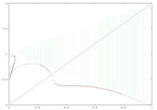
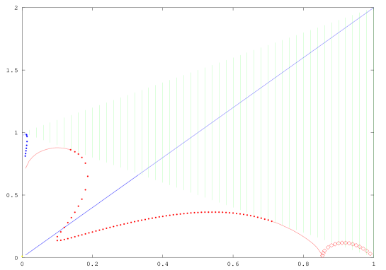
Figure 1: Gross–Neveu model, $k=2$ (the quintic case). Linearization at a solitary wave. Horizontal axis: $\omega\in(0,1)$. Vertical axis: spectrum on the upper half of the imaginary axis. Solid vertical (green) lines: part of the continuous spectrum between the threshold $i(1-|\omega|)$ and the embedded threshold $i(1+|\omega|)$. Solid red curves: eigenvalues with eigenfunctions from $\mathbf{X}$ (of the same parity as $\phi_{\omega}$; see (3.25)), which we can not ignore; our result holds in the regions where such eigenvalues are absent. Solid blue curve (near $\omega=0$ and $\lambda=i$) and the line $\lambda=2\omega i$ denote eigenvalues with eigenfunctions from $\mathbf{X}^{\perp}$ (see (3.26)), which remain orthogonal to our perturbation. Dotted red and blue curves: antibound states of different parity (from $\mathbf{X}$ and $\mathbf{X}^{\perp}$); we do not mention them in the argument. Antibound states correspond to zeros of Evans functions on the “wrong” Riemann sheet, which corresponds to generalized eigenfunctions with exponential growth at infinity.

Figure 2: Gross–Neveu model, $k=3$. Hollow red diamonds (on bottom right) denote positive eigenvalues (thus linear instability) present in the spectrum for $\omega\in(0.85,1)$. These eigenvalues are overimposed on the imaginary axis. Theorem 2.2 on asymptotic stability applies for solitary waves with $\omega$ such that there are neither hollow red diamonds (linear instability) nor solid red curves (purely imaginary eigenvalues with eigenfunctions from $\mathbf{X}$) in the spectrum. Note that the dotted kink indicates collision of antibound states at $\omega_{b}\approx 0.1$ on the imaginary axis and their bifurcation off the imaginary axis for $\omega<\omega_{b}$. (Location of these values of $\lambda$ off the imaginary axis does not lead to instability since the corresponding antibound states have infinite $L^{2}$-norm.)

Remark 2.7.

We discuss the necessary and sufficient conditions for the existence and properties of solitary waves in the generalized Gross–Neveu model in Section 3.1.

Remark 2.8.

By [Com11, CBS13], the assumptions $E(\omega)\neq 0$ and $\partial_{\omega}Q(\omega)\neq 0$ guarantee that the generalized null space of the linearization operator is (exactly) four-dimensional. (Above, $E(\omega)$ and $Q(\omega)$ are the values of the energy and charge functionals (2.6) (2.7) at the solitary wave $\phi_{\omega}e^{-i\omega t}$.) We do not need to impose the condition $E(\omega)\neq 0$ since although the vanishing of $E(\omega)$ leads to the increase of the Jordan block of the linearization operator, this increase is absent when we restrict the operator to the subspace $X$.

Remark 2.9.

The restriction of the linearized operator to $X$ requires some details. Since this operator is $\mathbb{R}$-linear but not $\mathbb{C}$-linear, by its restriction to $X$ we imply its restriction onto $\mathbf{X}=\mathbb{C}\otimes_{\mathbb{R}}(\mathop{\rm Re}X\times\mathop{\rm Im}X)$; see (3.25) below. More details are in Section 3.2.

Remark 2.10.

In Assumption 2.1, we require that $\varOmega\subset(-1/3,1/3)$ to avoid the situation when the eigenvalues $\pm 2\omega i$ (see Remark 3.5 below) become embedded into the essential spectrum ($\lambda\in i\mathbb{R}$, $\lvert\lambda\rvert\geq 1-\lvert\omega\rvert$). In that case, our construction of the resolvent in Section 4.2 does not allow to obtain the necessary estimates. Yet, the restriction to $\lvert\omega\rvert<1/3$ seems to be merely technical; we still expect that for $1/3\leq\lvert\omega\rvert<1$, the resolvent of the linearized operator restricted to $X$ has the same properties as stated in Proposition 4.14 even in the vicinity of the embedded eigenvalues $\pm 2\omega i$ and that the asymptotic stability could be proved.

Remark 2.11.

We expect that the Evans function never has zeros at $\lambda\in i\mathbb{R}$, $\lvert\mathop{\rm Im}\lambda\rvert\geq 1+\lvert\omega\rvert$, but could not prove this. Instead, we check this assumption numerically; all the zeros of the Evans function which we found are plotted as solid curves on Figures 2 and 2 (these zeros correspond to the point eigenvalues of the linearized operator). The absence of zeros of the Evans function for $\lambda\to\pm i\infty$ follows from Lemma 4.10.

Remark 2.12.

Let us summarize that most of our assumptions are technical; the only essential assumption is that the spectrum of the linearized operator has no eigenvalues in the right half-plane and that the Jordan block of $\lambda=0$ is (exactly) four-dimensional. We expect that the presence of purely imaginary eigenvalues does not lead to instability unless these eigenvalues are of higher algebraic multiplicity. More generally, we expect that, similarly to the case of the nonlinear Schrödinger equation and similar systems, the (dynamic) instability takes place when either there is a linear instability or when the eigenvalues on the imaginary axis are of higher algebraic multiplicities (when we are at the threshold of linear instability).

3 Solitary waves in generalized Gross–Neveu model

3.1 Properties of solitary waves

Equation (2.3) can be written explicitly as

$$\left\{\begin{array}[]{ll}i\partial_{t}\psi_{1}&=\partial_{x}\psi_{2}+\psi_{1}-f(|\psi_{1}|^{2}-|\psi_{2}|^{2})\psi_{1},\\ i\partial_{t}\psi_{2}&=-\partial_{x}\psi_{1}-\psi_{2}+f(|\psi_{1}|^{2}-|\psi_{2}|^{2})\psi_{2}.\end{array}\right.$$ (3.1)

In the abstract form, we write (2.3) as

$$i\partial_{t}\psi=D_{m}\psi+\mathbf{N}(\psi),$$ (3.2)

with the Dirac operator

$$D_{m}=-i\alpha\partial_{x}+\beta=\begin{bmatrix}1&\partial_{x}\\ -\partial_{x}&-1\end{bmatrix}$$

and the nonlinearity

$$\mathbf{N}(\psi)=\begin{bmatrix}-f(|\psi_{1}|^{2}-|\psi_{2}|^{2})&0\\ 0&f(|\psi_{1}|^{2}-|\psi_{2}|^{2})\end{bmatrix}\psi.$$ (3.3)

Definition 3.1.

Solitary waves are solutions of the form

$$\psi_{\omega}(x,t)=\phi_{\omega}(x)e^{-i\omega t},\qquad\phi_{\omega}\in H^{1}(\mathbb{R},\mathbb{C}^{2}),\qquad\omega\in\mathbb{R}.$$ (3.4)

Substituting this Ansatz into (3.2), we see that $\phi_{\omega}$ solves

$$\omega\phi_{\omega}=D_{m}\phi_{\omega}+\mathbf{N}(\phi_{\omega}).$$ (3.5)

The existence of solitary waves follows from [CV86, BC12a]:

Proposition 3.2.

Let $F(s)$ be the antiderivative of $f(s)$ such that $F(0)=0$. Assume that for given $\omega\in\mathbb{R}$, $0<\omega<1$, there exists $\varGamma_{\omega}>0$ such that

$$\omega\varGamma_{\omega}=\varGamma_{\omega}-F(\varGamma_{\omega}),\quad\omega\neq 1-f(\varGamma_{\omega}),\qquad\omega s<s-F(s),\qquad\text{for}\quad s\in(0,\varGamma_{\omega}).$$

Then there is a solitary wave solution $\psi_{\omega}(x,t)=\phi_{\omega}(x)e^{-i\omega t}$, where

$$\phi_{\omega}(x)=\begin{bmatrix}v(x,\omega)\\ u(x,\omega)\end{bmatrix},\qquad v(\cdot,\omega),\,u(\cdot,\omega)\in H^{1}(\mathbb{R}).$$ (3.6)

This solution is unique if we require that $v$, $u$ are real-valued, $v$ even and positive, and $u$ odd. Both $v$ and $u$ are exponentially decaying as $|x|\to\infty$ and satisfy $\lvert u(x,\omega)\rvert<\lvert v(x,\omega)\rvert$, $x\in\mathbb{R}$.

Moreover, there is $c_{\omega}<\infty$ such that

$$\lvert\phi_{\omega}(x)\rvert\leq c_{\omega}e^{-\updelta_{\omega}\lvert x\rvert},\qquad x\in\mathbb{R},$$ (3.7)

where

$$\updelta_{\omega}=\sqrt{1-\omega^{2}}.$$ (3.8)

Similarly, there is $c_{\omega}<\infty$ such that

$$\lvert\partial_{\omega}\phi_{\omega}(x)\rvert\leq c_{\omega}\langle x\rangle e^{-\updelta_{\omega}\lvert x\rvert},\qquad\lvert\partial_{\omega}^{2}\phi_{\omega}(x)\rvert\leq c_{\omega}\langle x\rangle^{2}e^{-\updelta_{\omega}\lvert x\rvert},\qquad x\in\mathbb{R}.$$ (3.9)

Proof.

The proof is given in e.g. [BC12a, Lemma 3.2]. The sharp rate of decay (3.7) can be proved as in e.g. [CCP07, Appendix A]. The bounds on $\lvert\partial_{\omega}\phi_{\omega}(x)\rvert$ and $\lvert\partial_{\omega}^{2}\phi_{\omega}(x)\rvert$ follow from differentiating (3.5) with respect to $\omega$. ∎

3.2 Linearization at a solitary wave

To study stability of a solitary wave $\phi_{\omega}(x)e^{-i\omega t}$, with $\phi_{\omega}(x)=\begin{bmatrix}v(x,\omega)\\ u(x,\omega)\end{bmatrix}\in\mathbb{R}^{2}$, we consider the solution in the form

$$\psi(x,t)=\big{(}\phi_{\omega}(x)+\rho(x,t)\big{)}e^{-i\omega t},\qquad\rho(x,t)\in\mathbb{C}^{2}.$$

Substituting this Ansatz into (3.2), we obtain:

$$i\partial_{t}\rho=(D_{m}-\omega I_{2})\rho+\mathbf{N}(\phi_{\omega}+\rho)-\mathbf{N}(\phi_{\omega}).$$ (3.10)

The linearization of (3.10) can be written as follows:

$$\dot{R}=\mathbf{J}\mathbf{L}R,\qquad R=\begin{bmatrix}\mathop{\rm Re}\rho\\ \mathop{\rm Im}\rho\end{bmatrix}\in\mathbb{R}^{4},$$ (3.11)

where

$$\mathbf{J}=\begin{bmatrix}0&I_{2}\\ -I_{2}&0\end{bmatrix},\qquad\mathbf{L}(\omega)=\mathbf{D}_{m}-\omega I_{4}+\mathbf{W}(x,\omega),$$ (3.12)

with

$$\mathbf{W}(x,\omega)=\begin{bmatrix}W_{1}(x,\omega)&0\\ 0&W_{0}(x,\omega)\end{bmatrix},$$ (3.13)

$$W_{0}(x,\omega)=\begin{bmatrix}-f(v^{2}-u^{2})&0\\ 0&f(v^{2}-u^{2})\end{bmatrix},\quad W_{1}(x,\omega)=W_{0}(x,\omega)-2f^{\prime}(v^{2}-u^{2})\begin{bmatrix}v^{2}&-vu\\ -vu&u^{2}\end{bmatrix}.$$

The free Dirac operator takes the form

$$\mathbf{D}_{m}=\mathbf{J}\bm{\upalpha}\partial_{x}+\bm{\upbeta},$$ (3.14)

with

$$\bm{\upalpha}=\begin{bmatrix}\mathop{\rm Re}\alpha&-\mathop{\rm Im}\alpha\\ \mathop{\rm Im}\alpha&\mathop{\rm Re}\alpha\end{bmatrix}=\begin{bmatrix}0&\mathop{\rm Im}\sigma_{2}\\ -\mathop{\rm Im}\sigma_{2}&0\end{bmatrix},\qquad\bm{\upbeta}=\begin{bmatrix}\mathop{\rm Re}\beta&-\mathop{\rm Im}\beta\\ \mathop{\rm Im}\beta&\mathop{\rm Re}\beta\end{bmatrix}=\begin{bmatrix}\sigma_{3}&0\\ 0&\sigma_{3}\end{bmatrix};$$ (3.15)

$\mathbf{J}$, $\bm{\upalpha}$, and $\bm{\upbeta}$ represent $-i$, $\alpha$, and $\beta$ when acting on $\begin{bmatrix}\mathop{\rm Re}\psi\\ \mathop{\rm Im}\psi\end{bmatrix}$, with $\psi\in\mathbb{C}^{2}$. We then have

$$\mathbf{D}_{m}=\begin{bmatrix}D_{m}&0\\ 0&D_{m}\end{bmatrix},\qquad\mbox{where}\quad D_{m}=\begin{bmatrix}1&\partial_{x}\\ -\partial_{x}&-1\end{bmatrix}.$$ (3.16)

Note that since $v,\,u$ both depend on $\omega$, the potentials $W_{1},W_{0}$ also depend on it. We will often omit this dependence in our notations.

Lemma 3.3.

There is $C_{\omega}<\infty$ such that the matrix-valued potential $\mathbf{W}$ satisfies

$$\left\|\mathbf{W}(x,\omega)\right\|_{\mathbb{C}^{4}\to\mathbb{C}^{4}}\leq C_{\omega}e^{-2k\lvert x\rvert\updelta_{\omega}},\qquad x\in\mathbb{R}.$$ (3.17)

Proof.

This bound is an immediate consequence of the exponential decay of $\phi_{\omega}$ in Proposition 3.2 (see (3.7)), the assumption $f(s)=\mathcal{O}(s^{k})$, and (3.13). ∎

Lemma 3.4.

$$\sigma_{\rm ess}(\mathbf{J}\mathbf{L})=i\mathbb{R}\backslash\big{(}-i(1-\lvert\omega\rvert),i(1-\lvert\omega\rvert)\big{)}.$$

Proof.

This is an immediate consequence of Weyl’s theorem on the essential spectrum. ∎

Denote

$$\bm{\upphi}(x)=\bm{\upphi}_{\omega}(x)=\begin{bmatrix}\mathop{\rm Re}\phi_{\omega}(x)\\ \mathop{\rm Im}\phi_{\omega}(x)\end{bmatrix}=\begin{bmatrix}\phi_{\omega}(x)\\ 0\end{bmatrix}.$$ (3.18)

Thanks to the invariance of (3.5) with respect to the phase rotation and the translation, we have

$$\mathbf{J}\mathbf{L}\mathbf{J}\bm{\upphi}=0,\qquad\mathbf{J}\mathbf{L}\partial_{x}\bm{\upphi}=0.$$

Analyzing the Jost solutions of

$$L_{1}(\omega)=D_{m}-\omega I_{2}+W_{1},\qquad L_{0}(\omega)=D_{m}-\omega I_{2}+W_{0}$$ (3.19)

(for each of $L_{1}$ and $L_{0}$, there are two Jost solutions: one decreasing and one increasing), one concludes that the null space of $\mathbf{L}$ is given by

$$N(\mathbf{L})=\left(\mathbf{J}\bm{\upphi},\ \partial_{x}\bm{\upphi}\right).$$ (3.20)

Moreover,

$$\mathbf{J}\mathbf{L}\partial_{\omega}\bm{\upphi}=\mathbf{J}\bm{\upphi},$$ (3.21)

$$\mathbf{J}\mathbf{L}\Big{(}\omega x\mathbf{J}\bm{\upphi}-\frac{1}{2}\bm{\upalpha}\bm{\upphi}\Big{)}=\partial_{x}\bm{\upphi},$$ (3.22)

where

$$\omega x\mathbf{J}\bm{\upphi}-\frac{1}{2}\bm{\upalpha}\bm{\upphi}=\begin{bmatrix}0\\ \frac{i}{2}\alpha\phi-\omega x\phi\end{bmatrix}=\begin{bmatrix}0\\ -\frac{i}{2}\sigma_{2}\phi-\omega x\phi\end{bmatrix}.$$

Therefore,

$$\left\{\mathbf{J}\bm{\upphi},\ \partial_{x}\bm{\upphi},\ \partial_{\omega}\bm{\upphi},\ \ \omega x\mathbf{J}\bm{\upphi}-\frac{1}{2}\bm{\upalpha}\bm{\upphi}\right\}\subset N_{g}(\mathbf{J}\mathbf{L}).$$ (3.23)

By [CBS13], if $\partial_{\omega}Q(\omega)$ and $E(\omega)\neq 0$, then the above vectors form a basis in the generalized null space $N_{g}(\mathbf{J}\mathbf{L})$:

$$N_{g}(\mathbf{J}\mathbf{L})=\mathop{\rm Span}\left(\mathbf{J}\bm{\upphi},\ \partial_{x}\bm{\upphi},\ \partial_{\omega}\bm{\upphi},\ \ \omega x\mathbf{J}\bm{\upphi}-\frac{1}{2}\bm{\upalpha}\bm{\upphi}\right).$$ (3.24)

Following the definition (2.8), we define

$$\mathbf{X}=\left\{\psi\in L^{2}(\mathbb{R},\mathbb{C}^{4});\;\ \psi_{k}(x)=\psi_{k}(-x),\ \ k=1,\,3;\quad\psi_{k}(x)=-\psi_{k}(-x),\ \ k=2,\,4\right\};$$ (3.25)

$$\mathbf{X}^{\perp}=\left\{\psi\in L^{2}(\mathbb{R},\mathbb{C}^{4});\;\ \psi_{k}(x)=\psi_{k}(-x),\ \ k=2,\,4;\quad\psi_{k}(x)=-\psi_{k}(-x),\ \ k=1\,3\right\}.$$ (3.26)

From now on, we shall restrict $\mathbf{J}\mathbf{L}(\omega)$ to $\mathbf{X}$. This restriction has the following null space and generalized null space:

$$N(\mathbf{J}\mathbf{L}|_{\mathbf{X}})=\mathop{\rm Span}\left(\mathbf{J}\bm{\upphi}\right),\qquad N_{g}(\mathbf{J}\mathbf{L}|_{\mathbf{X}})=\mathop{\rm Span}\left(\mathbf{J}\bm{\upphi},\ \partial_{\omega}\bm{\upphi}\right).$$ (3.27)

The linearization operator $\mathbf{J}\mathbf{L}$ acts invariantly in $\mathbf{X}$ and in $\mathbf{X}^{\perp}$.

Remark 3.5.

The restriction of $\mathbf{J}\mathbf{L}(\omega)$ onto $\mathbf{X}$ allows one to exclude certain eigenvalue directions, significantly simplifying the problem. In particular, by [Com11], one has

$$\mathbf{J}\mathbf{L}\begin{bmatrix}\sigma_{1}\phi\\ i\sigma_{1}\phi\end{bmatrix}=2i\omega\begin{bmatrix}\sigma_{1}\phi\\ i\sigma_{1}\phi\end{bmatrix},\qquad\mathbf{J}\mathbf{L}\begin{bmatrix}\sigma_{1}\phi\\ -i\sigma_{1}\phi\end{bmatrix}=-2i\omega\begin{bmatrix}\sigma_{1}\phi\\ -i\sigma_{1}\phi\end{bmatrix},$$ (3.28)

where $\sigma_{1}$ is the Pauli matrix; this shows that $\pm 2\omega i\in\sigma_{p}(\mathbf{J}\mathbf{L}(\omega))$. On the other hand, the restriction to $\mathbf{X}$ satisfies $\pm 2\omega i\not\in\sigma_{d}(\mathbf{J}\mathbf{L}|_{\mathbf{X}})$.

Since $(\mathbf{J}\mathbf{L})^{*}=-\mathbf{L}\mathbf{J}$, it follows from (3.21), (3.22) that the corresponding generalized kernel for the adjoint is

$$\mathbf{X}_{g}((\mathbf{J}\mathbf{L})^{*})=N_{g}((\mathbf{J}\mathbf{L})^{*})\cap\mathbf{X}=\left\{\ \mathbf{J}\partial_{\omega}\bm{\upphi},\bm{\upphi}\right\}.$$

We decompose the space $\mathbf{X}$ as follows:

$$\mathbf{X}=\mathbf{X}_{g}(\mathbf{J}\mathbf{L})\oplus\mathbf{X}_{c}(\mathbf{J}\mathbf{L}),\quad\text{where}\quad\mathbf{X}_{c}(\mathbf{J}\mathbf{L})=\mathbf{X}_{g}((\mathbf{J}\mathbf{L})^{*})^{\perp}.$$ (3.29)

The subspaces $\mathbf{X}_{g}(\mathbf{J}\mathbf{L})$ and $\mathbf{X}_{c}(\mathbf{J}\mathbf{L})$ are invariant under the action of $\mathbf{J}\mathbf{L}$, and any $R_{1}\in\mathbf{X}_{g}(\mathbf{J}\mathbf{L})$, $R_{2}\in\mathbf{X}_{c}(\mathbf{J}\mathbf{L})$ satisfy the following symplectic orthogonality condition:

$$\langle\mathbf{J}R_{1},R_{2}\rangle=0.$$

It then follows that any $R\in\mathbf{X}$ can be uniquely decomposed into

$$R=2\frac{\langle\bm{\upphi},R\rangle}{Q^{\prime}(\omega)}\partial_{\omega}\bm{\upphi}+2\frac{\langle\mathbf{J}\partial_{\omega}\bm{\upphi},R\rangle}{Q^{\prime}(\omega)}\mathbf{J}\bm{\upphi}+U,\qquad U\in\mathbf{X}_{c}(\mathbf{J}\mathbf{L}),$$ (3.30)

where $Q(\omega)$ is the charge functional (2.7) evaluated at $\phi_{\omega}e^{-i\omega t}$. Thus, a vector function $U\in X_{c}(\mathbf{J}\mathbf{L})$ satisfies the following two symplectic orthogonality conditions:

$$\langle\bm{\upphi},U\rangle=0,\qquad\langle\mathbf{J}\partial_{\omega}\bm{\upphi},U\rangle=0.$$ (3.31)

Remark 3.6.

Note that $Q^{\prime}(\omega)\neq 0$ by Assumption 2.1.

Let $P_{d}(\omega)$ denote the symplectically orthogonal projection onto the generalized null space of $\mathbf{J}\mathbf{L}(\omega)$ restricted onto the space $\mathbf{X}$ from (3.25). By (3.30),

$$P_{d}(\omega)R=2\frac{\langle\bm{\upphi},R\rangle}{Q^{\prime}(\omega)}\partial_{\omega}\bm{\upphi}+2\frac{\langle\mathbf{J}\partial_{\omega}\bm{\upphi},R\rangle}{Q^{\prime}(\omega)}\mathbf{J}\bm{\upphi},$$ (3.32)

while the projection onto $\mathbf{X}_{c}$ is

$$P_{c}(\omega)=1-P_{d}(\omega).$$ (3.33)

4 Spectral theory for the linearized operator

In this section, we consider dispersive estimates for the complexification of the linearized equation (3.11),

$$\partial_{t}R=\mathbf{J}\mathbf{L}R,\qquad R\in\mathbb{C}^{4}.$$ (4.1)

More precisely, we will show that similarly to the free Dirac evolution, the linear evolution of (4.1) projected onto the continuous spectrum of $\mathbf{J}\mathbf{L}$ scatters the initial data. This phenomena in the related Schrödinger equation context manifests itself in a variety of useful estimates; see for example the work of Mizumachi [Miz08].

Before proceeding to specific estimates for the solution of (3.11), let us take a moment to properly define $e^{\mathbf{J}\mathbf{L}t}P_{c}$. Since

$$\sigma_{\mathrm{ess}}(\mathbf{J}\mathbf{L}(\omega))=(-i\infty,-i(1-\lvert\omega\rvert)]\cup[i(1-\lvert\omega\rvert),i\infty),$$

we define $e^{\mathbf{J}\mathbf{L}(\omega)t}P_{c}(\omega)$ by the following Cauchy formula:

$$e^{\mathbf{J}\mathbf{L}t}P_{c}(\omega)f = -\frac{1}{2\pi i}\oint_{\Gamma}R_{\mathbf{J}\mathbf{L}}(\lambda)f\,d\lambda$$ (4.2)

$$= -\frac{1}{2\pi i}\left(\int_{-i\infty}^{-i(1-\lvert\omega\rvert)}+\int_{i(1-\lvert\omega\rvert)}^{i\infty}\right)e^{\lambda t}\Big{(}\big{[}R_{\mathbf{J}\mathbf{L}}^{+}(\lambda)-R_{\mathbf{J}\mathbf{L}}^{-}(\lambda)\big{]}f\Big{)}\,d\lambda$$

$$= -\frac{1}{2\pi}\left(\int_{-\infty}^{\lvert\omega\rvert-1}+\int_{1-\lvert\omega\rvert}^{+\infty}\right)e^{i\Lambda t}\Big{(}\big{[}R_{\mathbf{J}\mathbf{L}}^{+}(i\Lambda)-R_{\mathbf{J}\mathbf{L}}^{-}(i\Lambda)\big{]}f\Big{)}\,d\Lambda,$$

where $\Gamma$ is a positively-oriented contour around the essential spectrum of $\mathbf{J}\mathbf{L}$. For $\lambda\in i\mathbb{R}$ the operators

$$R_{\mathbf{J}\mathbf{L}}^{\pm}(\lambda):=\lim_{\varepsilon\to 0+}(\mathbf{J}\mathbf{L}-(\lambda\pm\varepsilon))^{-1}$$

are to be interpreted in a certain appropriate sense (for example, as operators from $L^{2}_{\alpha}\to L^{2}_{-\alpha}$, for certain $\alpha>0$, by the limiting absorption principle).

4.1 The Jost solutions and the Evans function of the linearization operator $\mathbf{J}\mathbf{L}$

The eigenvalue problem for the operator $\mathbf{J}\mathbf{L}(\omega)$,

$$\mathbf{J}(\mathbf{D}_{m}-\omega+\mathbf{W}(x,\omega))\psi=\mathbf{J}(\mathbf{J}\bm{\upalpha}\partial_{x}+\bm{\upbeta}-\omega+\mathbf{W}(x,\omega))\psi=\lambda\psi,$$

can be rewritten as

$$(\partial_{x}-\bm{\upalpha}\mathbf{J}\bm{\upbeta}+\omega\bm{\upalpha}\mathbf{J}+\bm{\upalpha}\lambda-\bm{\upalpha}\mathbf{J}\mathbf{W}(x,\omega)\big{)}\psi=0.$$ (4.3)

The construction of Jost solutions is based on considering solutions to the constant coefficient equation

$$(\partial_{x}-\mathcal{M}_{0}(\lambda,\omega)\big{)}\psi=0,\qquad\mathcal{M}_{0}(\lambda,\omega):=\bm{\upalpha}\mathbf{J}\bm{\upbeta}-\omega\bm{\upalpha}\mathbf{J}-\bm{\upalpha}\lambda,$$ (4.4)

and using the Duhamel representation to construct solutions to equation (4.3) with variable coefficients, written in the form

$$\big{(}\partial_{x}-\mathcal{M}(x,\lambda,\omega)\big{)}\psi=0,\qquad\mathcal{M}(x,\lambda,\omega):=\mathcal{M}_{0}(\lambda,\omega)+\bm{\upalpha}\mathbf{J}\mathbf{W}(x,\omega).$$ (4.5)

Lemma 4.1.

Let $\omega\in[-1,1]$, $\lambda\in\mathbb{C}$. Then the eigenvalues of $\mathcal{M}_{0}(\lambda,\omega)$ are given by

$$\sigma(\mathcal{M}_{0}(\lambda,\omega))=\{\pm\sqrt{1-(\omega\pm i\lambda)^{2}}\}.$$ (4.6)

These eigenvalues satisfy

$$\sup_{\lambda\in i\mathbb{R}}\big{\{}\lvert\mathop{\rm Re}\zeta\rvert;\ \zeta\in\sigma(\mathcal{M}_{0}(\lambda,\omega))\big{\}}=1;\qquad\sup_{\lambda\in\sigma_{\mathrm{ess}}(\mathbf{J}\mathbf{L}(\omega))}\big{\{}\lvert\mathop{\rm Re}\zeta\rvert;\ \zeta\in\sigma(\mathcal{M}_{0}(\lambda,\omega))\big{\}}=2\sqrt{\omega-\omega^{2}}.$$ (4.7)

Proof.

We need to find all $z\in\mathbb{C}$ such that

$$\mathcal{M}_{0}(\lambda,\omega)-z=\bm{\upalpha}\mathbf{J}\bm{\upbeta}-\omega\bm{\upalpha}\mathbf{J}-\bm{\upalpha}\lambda-z=-\bm{\upalpha}\lambda-\omega\bm{\upalpha}\mathbf{J}-z+\bm{\upalpha}\mathbf{J}\bm{\upbeta}$$

is degenerate. Multiplying the above matrix in the right-hand side by $-\bm{\upalpha}\mathbf{J}$, we need to find out when the matrix

$$\mathbf{J}\lambda-\omega+\bm{\upalpha}\mathbf{J}z+\bm{\upbeta}$$

is degenerate. Since $\bm{\upalpha}\bm{\upbeta}$ anticommutes with both $\bm{\upalpha}$ and $\bm{\upbeta}$, while $\det\bm{\upalpha}=\det\bm{\upbeta}=1$, one has:

$$\det(\mathbf{J}\lambda-\omega+\bm{\upalpha}\mathbf{J}z+\bm{\upbeta})^{2}=\det\big{(}(\mathbf{J}\lambda-\omega+\bm{\upalpha}\mathbf{J}z+\bm{\upbeta})\bm{\upalpha}\bm{\upbeta}(\mathbf{J}\lambda-\omega+\bm{\upalpha}\mathbf{J}z+\bm{\upbeta})\bm{\upbeta}\bm{\upalpha}\big{)}$$

$$=\det\big{(}(\mathbf{J}\lambda-\omega+\bm{\upalpha}\mathbf{J}z+\bm{\upbeta})(\mathbf{J}\lambda-\omega-\bm{\upalpha}\mathbf{J}z-\bm{\upbeta})\big{)}=\det\big{(}(\mathbf{J}\lambda-\omega)^{2}-(-z^{2}+1)\big{)}.$$

Since $\sigma(\mathbf{J})=\{\pm i\}$, we conclude that the above determinant vanishes (hence $z\in\sigma(\mathcal{M}_{0}(\lambda,\omega))$) if and only if

$$z^{2}-1+(\pm i\lambda-\omega)^{2}=0.$$

The conclusion about the spectrum of $\mathcal{M}_{0}$ follows.

Other statements are checked by direct computation. ∎

Due to the symmetry of the potential $\mathbf{W}$ (see (4.8) below), we have the following results.

Lemma 4.2.

If $\psi(x)$ solves (4.5) for $\lambda\in\mathbb{C}$, then $\theta(x)=\bm{\upbeta}\psi(-x)$ also solves (4.5) for the same $\lambda\in\mathbb{C}$.

Proof.

Since $v$ is even and $u$ is odd, and since $\beta=\sigma_{3}$ anticommutes with $\sigma_{1}$, there are the relations

$$W_{0}(x)\beta=\beta W_{0}(-x),\qquad W_{1}(x)\beta=\beta W_{1}(-x),$$ (4.8)

for $W_{0}$, $W_{1}$ from the Gross–Neveu model (3.13). (It is convenient to notice that for each of these models, $W_{0}$ and $W_{1}$ can be written as linear combinations of the form $w_{a}(x)\sigma_{1}+w_{b}(x)\sigma_{3}+w_{c}(x)I_{2}$, with scalar-valued functions $w_{b}$ and $w_{c}$ symmetric in $x$ and $w_{a}$ skew-symmetric.) The conclusion follows. ∎

Lemma 4.3.

For any $x\in\mathbb{R}$, $\omega\in\varOmega$, and $\lambda\in\mathbb{C}$, the matrix $\mathcal{M}$ from (4.5) satisfies one has $\mathop{\rm tr}\mathcal{M}(x,\lambda,\omega)=0$.

Proof.

The statement is immediate for all the terms from $\mathcal{M}_{0}$ (Cf. (4.4)). The remaining relation $\mathop{\rm tr}\bm{\upalpha}\mathbf{J}\mathbf{W}=0$ is checked with the explicit expressions (3.13). ∎

We now turn to the construction of the Jost solutions, which are defined as eigenfunctions of $\mathbf{J}\mathbf{L}(\omega)$ with the same asymptotic behavior as eigenfunctions of $\mathbf{J}(\mathbf{D}_{m}-\omega)$. To do this, for $\lambda\in\mathbb{C}$, we first define

$$\xi_{1}(\lambda,\omega)=\sqrt{(\omega-i\lambda)^{2}-1},\qquad\xi_{2}(\lambda,\omega)=\sqrt{(\omega+i\lambda)^{2}-1},$$ (4.9)

so that $\sigma(\mathcal{M}_{0}(\lambda,\omega))=\{\pm\xi_{1}(\lambda,\omega),\,\pm\xi_{2}(\lambda,\omega)\}$ (Cf. Lemma 4.1). Without loss of generality, we will only consider the case

$$\omega\geq 0,\qquad\mathop{\rm Re}\lambda\leq 0,\qquad\mathop{\rm Im}\lambda\geq 0;$$ (4.10)

in each of the two square roots in (4.9), we choose the branch that is positive for $\lambda\in i\mathbb{R}$, $\mathop{\rm Im}\lambda\gg 1$.

We define

$$\Xi_{1}(\lambda,\omega)=\frac{1}{c_{1}(\lambda,\omega)}\begin{bmatrix}i\xi_{1}\\ -i\lambda-1+\omega\\ -\xi_{1}\\ \lambda-i(1-\omega)\end{bmatrix},\qquad\mathrm{H}_{1}(\lambda,\omega)=\frac{1}{c_{1}(\lambda,\omega)}\begin{bmatrix}i\xi_{1}\\ i\lambda+1-\omega\\ -\xi_{1}\\ -\lambda+i(1-\omega)\end{bmatrix},$$ (4.11)

$$\Xi_{2}(\lambda,\omega)=\frac{1}{c_{2}(\lambda,\omega)}\begin{bmatrix}i\xi_{2}\\ i\lambda-1+\omega\\ \xi_{2}\\ \lambda+i(1-\omega)\end{bmatrix},\qquad\mathrm{H}_{2}(\lambda,\omega)=\frac{1}{c_{2}(\lambda,\omega)}\begin{bmatrix}i\xi_{2}\\ -i\lambda+1-\omega\\ \xi_{2}\\ -\lambda-i(1-\omega)\end{bmatrix},$$ (4.12)

with the constants

$$c_{1}(\lambda,\omega)>0,\qquad c_{2}(\lambda,\omega)>0$$ (4.13)

chosen so that $\lvert\Xi_{j}\rvert=\lvert\mathrm{H}_{j}\rvert=1$, $\ j=1,\,2$. Note that $\mathrm{H}_{j}=\bm{\upbeta}\Xi_{j}$; $j=1,\,2$. The functions

$$\Xi_{1}(\lambda,\omega)e^{i\xi_{1}(\lambda,\omega)x},\qquad\Xi_{2}(\lambda,\omega)e^{i\xi_{2}(\lambda,\omega)x},\qquad\mathrm{H}_{1}(\lambda,\omega)e^{-i\xi_{1}(\lambda,\omega)x},\qquad\mathrm{H}_{2}(\lambda,\omega)e^{-i\xi_{2}(\lambda,\omega)x}$$

satisfy the equation $(\mathbf{J}(\mathbf{D}_{m}-\omega)-\lambda)\psi(x)=0$ (and thus (4.4)).

By (4.10), we see that

$$\xi_{1}>\xi_{2}\geq 0\quad\text{for}\quad\lambda\in i\mathbb{R},\ \ \lvert\lambda\rvert\geq 1+\lvert\omega\rvert;\qquad\lvert\xi_{2}\rvert>\lvert\xi_{1}\rvert\quad\text{for}\quad\lambda\in i\mathbb{R},\ \ \lvert\lambda\rvert\leq 1-\lvert\omega\rvert.$$

We denote

$$\kappa_{1}=\lvert\mathop{\rm Im}\xi_{1}\rvert,\qquad\kappa_{2}=\lvert\mathop{\rm Im}\xi_{2}\rvert;$$ (4.14)

then one has

$$\kappa_{2}>\kappa_{1}\geq 0\qquad\mbox{for}\quad\lambda\in i\mathbb{R},\quad\lvert\lambda\rvert\leq 1-\lvert\omega\rvert.$$

Proposition 4.4.

Let $\omega\in\varOmega$. There are the Jost solutions $\mathbf{f}_{j}(x,\lambda,\omega)$, $\mathbf{g}_{j}(x,\lambda,\omega)$, $\mathbf{F}_{j}(x,\lambda,\omega)$, $\mathbf{G}_{j}(x,\lambda,\omega)$, $j=1,\,2$, which satisfy the equation $(\mathbf{J}\mathbf{L}(\omega)-\lambda)u=0$ and have the following properties. There is $c(\omega)<\infty$ such that

• For $\lambda\in i\mathbb{R}$, $\lvert\lambda\rvert\leq 1-\lvert\omega\rvert$,

  $$\lvert e^{\kappa_{j}x}\mathbf{f}_{j}(x,\lambda,\omega)-\Xi_{j}(\lambda,\omega)\rvert+\lvert e^{-\kappa_{j}x}\mathbf{F}_{j}(x,\lambda,\omega)-\mathrm{H}_{j}(\lambda,\omega)\rvert\leq c(\omega)e^{-2k\updelta_{\omega}x},\qquad x\geq 0,\qquad j=1,\,2.$$ (4.15)

• For $\lambda\in i\mathbb{R}$, $1-\lvert\omega\rvert\leq\lvert\lambda\rvert\leq 1+\lvert\omega\rvert$,

  $$\lvert e^{-i\xi_{1}x}\mathbf{f}_{1}(x,\lambda,\omega)-\Xi_{1}(\lambda,\omega)\rvert+\lvert e^{i\xi_{1}x}\mathbf{F}_{1}(x,\lambda,\omega)-\mathrm{H}_{1}(\lambda,\omega)\rvert\leq c(\omega)e^{-2k\updelta_{\omega}x},\qquad x\geq 0,$$

  $$\lvert e^{\kappa_{2}x}\mathbf{f}_{2}(x,\lambda,\omega)-\Xi_{2}(\lambda,\omega)\rvert+\lvert e^{-\kappa_{2}x}\mathbf{F}_{2}(x,\lambda,\omega)-\mathrm{H}_{2}(\lambda,\omega)\rvert\leq c(\omega)e^{-2k\updelta_{\omega}x},\qquad x\geq 0.$$

• For $\lambda\in i\mathbb{R}$, $\lvert\lambda\rvert\geq 1+\lvert\omega\rvert$,

  $$\lvert e^{-i\xi_{j}x}\mathbf{f}_{1}(x,\lambda,\omega)-\Xi_{j}(\lambda,\omega)\rvert+\lvert e^{i\xi_{j}x}\mathbf{F}_{1}(x,\lambda,\omega)-\mathrm{H}_{j}(\lambda,\omega)\rvert\leq c(\omega)e^{-2k\updelta_{\omega}x},\qquad x\geq 0,\qquad j=1,\,2.$$

• For $\lambda\in i\mathbb{R}$,

  $$\lvert\mathbf{f}_{j}(x,\lambda,\omega)\rvert+\lvert\mathbf{F}_{j}(x,\lambda,\omega)\rvert\leq c(\omega)\big{(}\langle x\rangle+e^{\kappa_{2}\lvert x\rvert}\big{)},\qquad x\leq 0,\qquad j=1,\,2.$$

• For $\lambda\in i\mathbb{R}$, $\lvert\lambda\rvert\geq 3$,

  $$\lvert\mathbf{f}_{j}(x,\lambda,\omega)\rvert+\lvert\mathbf{F}_{j}(x,\lambda,\omega)\rvert\leq c(\omega),\qquad x\in\mathbb{R},\qquad j=1,\,2.$$ (4.16)

• One can define the Jost solutions with appropriate asymptotics as $x\to-\infty$ by

  $$\mathbf{g}_{j}(x)=\bm{\upbeta}\mathbf{f}_{j}(-x),\qquad\mathbf{G}_{j}(x)=\bm{\upbeta}\mathbf{F}_{j}(-x),\qquad x\in\mathbb{R},\qquad j=1,\,2.$$ (4.17)

Above, $\updelta_{\omega}=\sqrt{1-\omega^{2}}$ (Cf. (3.8)).

Proof.

The proof is quite standard. However, since the decay rate of the potential $\mathbf{W}$ depends on $\omega$ and $k$ (Cf. Assumption 2.1), we choose to provide the details. Given $\varkappa\in\sigma(\mathcal{M}_{0}(\lambda,\omega))$, with $\omega\in\varOmega$ and $\lambda\in i\mathbb{R}$, let $\Xi\in\mathbb{C}^{4}$ be a corresponding eigenvector, with $\lvert\Xi\rvert=1$. To find a solution $\psi(x)\sim\Xi e^{\varkappa x}$, $x\to+\infty$ of (4.4), we define $\xi(x)$ by

$$\psi(x)=e^{\varkappa x}\xi(x),\qquad\text{so that}\quad\xi|_{x=+\infty}=\Xi;$$

then $\partial_{x}\xi=(\mathcal{M}_{0}-\varkappa)\xi+\bm{\upalpha}\mathbf{J}\mathbf{W}\xi,$ and hence we can write

$$\partial_{x}(e^{-(\mathcal{M}_{0}-\varkappa)x}\xi)=e^{-(\mathcal{M}_{0}-\varkappa)x}\bm{\upalpha}\mathbf{J}\mathbf{W}\xi.$$

We construct $\xi(x)$ in the form of the power series $\xi(x)=\sum_{n=0}^{\infty}\xi_{n}(x),$ where $\xi_{0}=\Xi$ and

$$\partial_{x}(e^{-(\mathcal{M}_{0}-\varkappa)x}\xi_{n}(x))=e^{-(\mathcal{M}_{0}-\varkappa)x}\bm{\upalpha}\mathbf{J}\mathbf{W}(x,\omega)\xi_{n-1}(x),\qquad\xi_{n}(+\infty)=0,\qquad n\geq 1;$$

hence

$$\xi_{n}(x)=-\int_{x}^{+\infty}e^{(\mathcal{M}_{0}-\varkappa)(x-y)}\bm{\upalpha}\mathbf{J}\mathbf{W}(y,\omega)\xi_{n-1}(y)\,dy,\qquad n\geq 1.$$

Let $P_{\zeta}$ denote the Riesz projector onto the eigenspace corresponding to $\zeta\in\sigma(\mathcal{M}_{0})$. Then, for $x\geq 0$,

$$\lvert P_{\zeta}\xi_{n}(x)\rvert \leq \int_{x}^{+\infty}\left\|P_{\zeta}e^{(\mathcal{M}_{0}-\varkappa)(x-y)}\right\|\left\|\mathbf{W}(y,\omega)\right\|_{\mathop{\mathrm{End}}(\mathbb{C}^{4})}\lvert\xi_{n-1}(y)\rvert\,dy$$ (4.18)

$$\leq \sup_{y\geq x}\lvert\xi_{n-1}(y)\rvert\int_{x}^{+\infty}ae^{(x-y)\mathop{\rm Re}(\zeta-\varkappa)}\langle x-y\rangle Ke^{-2k\updelta_{\omega}y}\,dy\leq ce^{-2k\updelta_{\omega}x}\sup_{y\geq x}\lvert\xi_{n-1}(y)\rvert,$$

for some $c=c(\omega,K)<\infty$. Above, we used the bound $\left\|P_{\zeta}e^{(\mathcal{M}_{0}-\varkappa)x}\right\|\leq ae^{x\mathop{\rm Re}(\zeta-\varkappa)}\langle x\rangle$, with some $a<\infty$ (which depends on $\omega$ but does not depend on $\zeta$), with the factor $\langle x\rangle$ due to the possibility of the Jordan block of $\mathcal{M}_{0}$ (when $\zeta=0$). For the convergence of the integration in $y$, we used the bound (3.17) and the inequalities

$$\lvert\mathop{\rm Re}\zeta\rvert\leq k\updelta_{\omega},\qquad\lvert\mathop{\rm Re}\varkappa\rvert\leq k\updelta_{\omega},$$ (4.19)

which are trivially satisfied under conditions of Assumption 2.1: one has $k\geq 2$, $\lvert\omega\rvert<1/3$, hence $k\updelta_{\omega}\geq 2\sqrt{8/9}$, while $\zeta\in\sigma(\mathcal{M}_{0}(\lambda,\omega))$ for any $\lambda\in i\mathbb{R}$, $\omega\in(-1,1)$, satisfy $\lvert\mathop{\rm Re}\zeta\rvert\leq 1$ (Cf. Lemma 4.1).

Then the integration in $y$ in (4.18) can be estimated as follows:

$$\int_{x}^{+\infty}e^{(x-y)\mathop{\rm Re}(\zeta-\varkappa)}\langle x-y\rangle e^{-2k\updelta_{\omega}y}\,dy=e^{-2k\updelta_{\omega}x}\int_{0}^{+\infty}e^{-z\mathop{\rm Re}(\zeta-\varkappa)}\langle z\rangle e^{-2k\updelta_{\omega}z}\,dz$$

$$\leq e^{-2k\updelta_{\omega}x}\Big{(}\frac{1}{2(k-1)\updelta_{\omega}}+\frac{1}{(2(k-1)\updelta_{\omega})^{2}}\Big{)}.$$

We conclude that

$$\sup_{y\geq x}\lvert\xi_{n}(y)\rvert=\sup_{y\geq x}\left\lvert\sum_{\zeta\in\sigma(\mathcal{M}_{0})}P_{\zeta}\xi_{n}(y)\right\rvert\leq\sum_{\zeta\in\sigma(\mathcal{M}_{0})}\sup_{y\geq x}\lvert P_{\zeta}\xi_{n}(y)\rvert\leq 4ce^{-2k\updelta_{\omega}x}\sup_{y\geq x}\lvert\xi_{n-1}(y)\rvert,\qquad x\geq 0.$$

Therefore, there is $C<\infty$ such that $\sum_{n=1}^{\infty}\lvert\xi_{n}(x)\rvert\leq Ce^{-2k\updelta_{\omega}x},$ for all $x\geq 0$, hence

$$\lvert\xi(x)-\Xi\rvert=Ce^{-2k\updelta_{\omega}x},\qquad x\geq 0.$$

Let us prove the uniform bounds (4.16). Let us write (4.5) in the form

$$(\partial_{x}-\mathcal{M}_{0}(\lambda,\omega))\psi=\bm{\upalpha}\mathbf{J}\mathbf{W}(x,\omega)\psi.$$ (4.20)

Using the Green function for the operator $\partial_{x}-\mathcal{M}_{0}(\lambda,\omega)$, which is given by

$$\mathscr{G}(x,y,\lambda,\omega)=\left(\Xi_{1}\otimes\theta_{1}^{\ast}e^{i(x-y)\xi_{1}}+\Xi_{2}\otimes\theta_{2}^{\ast}e^{i(x-y)\xi_{2}}+\mathrm{H}_{1}\otimes\eta_{1}^{\ast}e^{-i(x-y)\xi_{1}}+\mathrm{H}_{2}\otimes\eta_{2}^{\ast}e^{-i(x-y)\xi_{2}}\right)\Theta(x-y),$$

where $\Theta$ is the Heaviside step-function and $\theta_{j},\,\eta_{j}\in\mathbb{C}^{4}$, $j=1,\,2$, is the basis dual to $\Xi_{j},\,\mathrm{H}_{j}\in\mathbb{C}^{4}$, one can construct the solutions $\mathbf{f}_{j}(x,\lambda,\omega)$, $\mathbf{F}_{j}(x,\lambda,\omega)$, in the form of the power series

$$\psi=\sum_{n=0}^{\infty}\psi_{n},$$ (4.21)

with $\psi_{0}(x)=\Xi_{j}e^{i\xi_{j}x}$ or $\psi_{0}(x)=\mathrm{H}_{j}e^{-i\xi_{j}x}$ (according to (4.17), these are asymptotics of $\mathbf{f}_{j}(x),\,\mathbf{F}_{j}(x)$ for $x\gg 1$), and with $\psi_{n}(x)$, $n\geq 1$ solving

$$(\partial_{x}-\mathcal{M}_{0}(\lambda,\omega))\psi_{n}(x)=\bm{\upalpha}\mathbf{J}\mathbf{W}(x,\omega)\psi_{n-1}(x).$$

For definiteness, we will consider $\mathbf{f}_{1}(x)$ only (other functions are considered in the same way). For any $x\in\mathbb{R}$, the series (4.21) converges due to the estimate

$$\lvert\psi_{n}(x)\rvert \leq \int_{x}^{\infty}\left\|\mathbf{W}(x_{1})\right\|_{\mathop{\mathrm{End}}(\mathbb{C}^{4})}\lvert\psi_{n-1}(x_{1})\rvert\,dx_{1}$$

$$\leq \int_{x}^{\infty}\int_{x_{1}}^{\infty}\Big{\|}\mathbf{W}(x_{1})\Big{\|}_{\mathop{\mathrm{End}}(\mathbb{C}^{4})}\Big{\|}\mathbf{W}(x_{2})\Big{\|}_{\mathop{\mathrm{End}}(\mathbb{C}^{4})}\lvert\psi_{n-2}(x_{2})\rvert\,dx_{1}\,dx_{2}\leq\dots$$

$$\leq \mathop{\int\dots\int}_{x<x_{1}<\dots<x_{n}<\infty}\Big{(}\prod_{l=1}^{n}\left\|\mathbf{W}(x_{l})\right\|_{\mathop{\mathrm{End}}(\mathbb{C}^{4})}\Big{)}\lvert\psi_{0}(x_{n})\rvert\,dx_{1}\dots dx_{n}$$

$$\leq \frac{1}{n!}\int_{x_{1}>x}\dots\int_{x_{n}>x}\Big{(}\prod_{l=1}^{n}\left\|\mathbf{W}(x_{l})\right\|_{\mathop{\mathrm{End}}(\mathbb{C}^{4})}\Big{)}\lvert\psi_{0}(x_{n})\rvert\,dx_{1}\dots dx_{n}\leq\frac{(\int_{x}^{\infty}\left\|\mathbf{W}(y)\right\|_{\mathop{\mathrm{End}}(\mathbb{C}^{4})}\,dy)^{n}}{n!},$$

where we represented the integration over the simplex $x<x_{1}<\dots<x_{n}<\infty$ in $\mathbb{R}^{n}$ as a fraction of the integration over the quadrant $x_{l}>x$, $1\leq l\leq n$, and substituted $\lvert\psi_{0}(x_{n})\rvert=\lvert\Xi_{1}\rvert=1$. Therefore, $\lvert\psi(x)\rvert\leq\sum_{n\geq 0}\lvert\psi_{n}(x)\rvert\leq\mathop{\rm exp}\left(\int_{\mathbb{R}}\left\|\mathbf{W}(y)\right\|_{\mathop{\mathrm{End}}(\mathbb{C}^{4})}\,dy\right),$ for any $x\in\mathbb{R}$. This proves (4.16).

Finally, Lemma 4.2 allows to use (4.17) to obtain the Jost solutions with required asymptotic behaviour at $-\infty$. ∎

Definition 4.5.

We define the Evans function by

$$E(\lambda,\omega)=\det\big{[}\mathbf{f}_{1}(x,\lambda,\omega),\mathbf{f}_{2}(x,\lambda,\omega),\mathbf{g}_{1}(x,\lambda,\omega),\mathbf{g}_{2}(x,\lambda,\omega)\big{]}.$$ (4.22)

By Lemma 4.3 and Liouville’s formula, the right-hand side of (4.22) does not depend on $x\in\mathbb{R}$.

Lemma 4.6.

Fix $\omega\in\varOmega$.

1. Let $\lambda\in i\mathbb{R}$, $\lvert\lambda\rvert\in(1-\lvert\omega\rvert,1+\lvert\omega\rvert)$. Then $E(\lambda,\omega)=0$ at some $\lambda\in i\mathbb{R}$, $\lvert\lambda\rvert\in(1-\lvert\omega\rvert,1+\lvert\omega\rvert)$, if and only if $\lambda$ is an $L^{2}$ eigenvalue of $\mathbf{J}\mathbf{L}$.

2. At $\lambda=\pm i(1+\lvert\omega\rvert)$, one has $E(\lambda,\omega)=0$ only if there is a generalized $L^{\infty}$-eigenfunction corresponding to $\lambda$, which has the asymptotics $\psi\sim a\Xi_{2}$ as $x\to+\infty$, $\psi\sim b\mathrm{H}_{2}$ as $x\to-\infty$.

Remark 4.7.

The statement of the lemma at the thresholds is non-trivial since at the threshold points the solution to $(\mathbf{J}\mathbf{L}-\lambda)\psi=0$ which is bounded for $x\to+\infty$ could be linearly growing as $x\to-\infty$.

Proof.

Let us prove Part 1. Consider the case $\pm\lambda\in i(1-\lvert\omega\rvert,1+\lvert\omega\rvert)$. Due to the asymptotics of the Jost solutions, if $\mathbf{f}_{1}$ and $\mathbf{g}_{1}$ are linearly dependent, then $\mathbf{f}_{1}=C\mathbf{g}_{1}=\psi$ is the exponentially decaying solution to (4.5) and thus $\lambda$ is an $L^{2}$ eigenvalue. This proves the “if” statement of the lemma.

Let us prove the converse statement. If $\det[\mathbf{f}_{1},\mathbf{f}_{2},\mathbf{g}_{1},\mathbf{g}_{2}]=0$ for some $\lambda\in i\mathbb{R}$, then there are $a_{1},\,a_{2},\,b_{1},\,b_{2}\in\mathbb{C}$, not all of them equal to zero, one has

$$\varPhi(x):=\sum_{j=1}^{2}a_{j}\mathbf{f}_{j}(x,\lambda,\omega)=\sum_{j=1}^{2}b_{j}\mathbf{g}_{j}(x,\lambda,\omega),\qquad x\in\mathbb{R}.$$ (4.23)

Clearly, $\varPhi$ thus defined is not identically zero.

Define

$$\varSigma=i\mathbf{J}=\begin{bmatrix}0&iI_{2}\\ -iI_{2}&0\end{bmatrix}.$$

Let us consider the auxiliary Dirac equation

$$i\varSigma\partial_{t}\Psi=\mathbf{L}\Psi,\qquad\Psi(x,t)\in\mathbb{C}^{4},\quad x\in\mathbb{R},$$ (4.24)

where $\mathbf{L}=\mathbf{J}\bm{\upalpha}\partial_{x}+\bm{\upbeta}+\mathbf{W}-\omega.$ This is a Hamiltonian system with the Hamiltonian density

$$\eur{h}=\Psi^{\ast}\mathbf{L}\Psi=\Psi^{\ast}(\mathbf{J}\bm{\upalpha}\partial_{x}+\bm{\upbeta}+\mathbf{W}-\omega)\Psi$$

and the Lagrangian density

$$\eur{l}=\Psi^{\ast}(i\varSigma\partial_{t}-\mathbf{L})\Psi.$$

If $\varPhi\in C^{1}(\mathbb{R},\mathbb{C}^{4})$ satisfies $\lambda\varPhi=\mathbf{J}\mathbf{L}\varPhi$, which we write as $(i\lambda)(i\mathbf{J})\varPhi=-\lambda\mathbf{J}\varPhi=\mathbf{L}\varPhi$, then we have

$$\Omega\varSigma\varPhi=\mathbf{L}\varPhi,\qquad\Omega:=i\lambda\in\mathbb{R}.$$

Thus, $\Psi(x,t)=\varPhi(x)e^{-i\Omega t}$ is a “solitary wave solution” to (4.24), except that $\varPhi$ is not necessarily in $L^{2}$.

Equation (4.24) conserves the Krein charge; its density is

$$\sigma(x,t)=\Psi^{\ast}\varSigma\Psi=\varPhi^{\ast}\varSigma\varPhi,$$ (4.25)

while the density of the corresponding current is

$$\eur{j}(x,t)=\Psi^{\ast}\varSigma\bm{\upalpha}\Psi=\varPhi^{\ast}\varSigma\bm{\upalpha}\varPhi.$$ (4.26)

Remark 4.8.

We call the quantity $\langle\Psi,\varSigma\Psi\rangle$ the “Krein charge” in view of its relation to the Krein index considerations. Namely, the relation $\mathbf{J}\mathbf{L}\varPhi=\lambda\varPhi$ implies that $\langle\varPhi,\mathbf{L}\varPhi\rangle=-\lambda\langle\varPhi,\mathbf{J}\varPhi\rangle$, with $\langle\varPhi,\mathbf{L}\varPhi\rangle$ real and $\langle\varPhi,\mathbf{J}\varPhi\rangle$ purely imaginary; hence $\mathop{\rm Re}\lambda\neq 0$ leads to $\langle\varPhi,\mathbf{J}\varPhi\rangle=0$, $\langle\varPhi,\mathbf{L}\varPhi\rangle=0$. Thus, the Krein signature is zero ($\mathbf{L}$ is not sign-definite on the corresponding eigenspace) for any eigenvalue away from the imaginary axis. (The above could also be interpreted as follows. We could say that if $\Psi=\varPhi(x)e^{-i\Omega t}$ (with $\Omega=i\lambda$) is a solitary wave solution to (4.24) and $\mathop{\rm Im}\Omega=\mathop{\rm Re}\lambda\neq 0$, then the conservation of the “Krein charge” $\langle\Psi(t),\varSigma\Psi(t)\rangle=\langle\varPhi,\varSigma\varPhi\rangle e^{2\mathop{\rm Im}\Omega t}$ requires that this charge is zero, $\langle\varPhi,\varSigma\varPhi\rangle=0$.) It follows that purely imaginary eigenvalues $\lambda\in i\mathbb{R}\setminus 0$ with nonzero Krein signature, $\langle\varPhi,i\mathbf{J}\varPhi\rangle\neq 0$, can not bifurcate off the imaginary axis into the complex plane.

Since the Krein charge density does not depend on time, the local conservation of the Krein charge in the system (4.24) leads to the equality of the Krein current (4.26) evaluated at the endpoints of the interval $(-l,l)$, $l>0$. Therefore, taking into account that

$$\varSigma\Xi_{1}=-\Xi_{1},\qquad\varSigma\Xi_{2}=\Xi_{2},\qquad\varSigma\mathrm{H}_{1}=-\mathrm{H}_{1},\qquad\varSigma\mathrm{H}_{2}=\mathrm{H}_{2},$$

we compute for $\varPhi$ from (4.23):

$$0=\lim_{l\to+\infty}\varPhi^{\ast}\varSigma\bm{\upalpha}\varPhi|^{l}_{-l}=\lim_{l\to+\infty}\big{(}(a_{1}\Xi_{1}e^{i\xi_{1}x}+a_{2}\Xi_{2}e^{-\kappa_{2}x})^{\ast}\bm{\upalpha}(-a_{1}\Xi_{1}e^{i\xi_{1}x}+a_{2}\Xi_{2}e^{-\kappa_{2}x})\big{)}|_{x=l}$$

$$-\lim_{l\to+\infty}\big{(}(b_{1}\mathrm{H}_{1}e^{-i\xi_{1}x}+b_{2}\mathrm{H}_{2}e^{-\kappa_{2}\lvert x\rvert})^{\ast}\bm{\upalpha}(-b_{1}\mathrm{H}_{1}e^{-i\xi_{1}x}+b_{2}\mathrm{H}_{2}e^{-\kappa_{2}\lvert x\rvert})\big{)}|_{x=-l}$$

$$=\lim_{l\to+\infty}\big{(}(a_{1}\Xi_{1}e^{i\xi_{1}x}+a_{2}\Xi_{2}e^{-\kappa_{2}x})^{\ast}\bm{\upalpha}(-a_{1}\Xi_{1}e^{i\xi_{1}x}+a_{2}\Xi_{2}e^{-\kappa_{2}x})\big{)}|_{x=l}$$

$$-\lim_{l\to+\infty}\big{(}(b_{1}\Xi_{1}e^{-i\xi_{1}x}+b_{2}\Xi_{2}e^{-\kappa_{2}\lvert x\rvert})^{\ast}\bm{\upalpha}(b_{1}\Xi_{1}e^{-i\xi_{1}x}-b_{2}\Xi_{2}e^{-\kappa_{2}\lvert x\rvert})\big{)}|_{x=-l}.$$ (4.27)

In the last relation, we took into account that $\mathrm{H}_{j}=\bm{\upbeta}\Xi_{j}$ and that $\bm{\upbeta}$ anticommutes with $\bm{\upalpha}$. Taking into account that $\Xi_{1}^{\ast}\bm{\upalpha}\Xi_{2}=\Xi_{2}^{\ast}\bm{\upalpha}\Xi_{1}=0$, we rewrite the above as

$$0=(\lvert a_{1}\rvert^{2}+\lvert b_{1}\rvert^{2})\Xi_{1}^{\ast}\bm{\upalpha}\Xi_{1}+(\lvert a_{2}\rvert^{2}+\lvert b_{2}\rvert^{2})\Xi_{2}^{\ast}\bm{\upalpha}\Xi_{2}\lim_{l\to+\infty}e^{-2\kappa_{2}l}.$$ (4.28)

For Part 1, when $\lambda\in i\mathbb{R}$ and $1-\lvert\omega\rvert<\lvert\lambda\rvert<1+\lvert\omega\rvert$, one has $\kappa_{2}>0$, hence the second term in the right-hand side of (4.28) vanishes. On the other hand,

$$\Xi_{1}^{\ast}\bm{\upalpha}\Xi_{1}=\frac{4i(\lambda-i(1-\omega))\xi_{1}}{c_{1}^{2}}>0\qquad\mbox{for}\quad\lambda\in i\mathbb{R},\ \ \mathop{\rm Im}\lambda>1-\lvert\omega\rvert.$$

Then it follows from (4.28) that $a_{1}=b_{1}=0$, and we conclude that $\varPhi$ is exponentially decaying for $x\to\pm\infty$, so that $\lambda$ is an $L^{2}$ eigenvalue. This finishes the proof of Part 1.

For Part 2, when $\lambda=\pm(1+\lvert\omega\rvert)i$, one has $\kappa_{2}=0=\xi_{2}$, and, using (4.12), one computes

$$\Xi_{2}^{\ast}\bm{\upalpha}\Xi_{2}=\frac{4i(\lambda+i(1-\omega))\xi_{2}}{c_{2}^{2}}=0;$$

therefore, (4.28) again yields $a_{1}=b_{1}=0$. ∎

For $\lambda\in i\mathbb{R}$, $\lvert\lambda\rvert>1+\lvert\omega\rvert$, the functions $\mathbf{f}_{1}(\lambda,\omega)$, $\mathbf{f}_{2}(\lambda,\omega)$, $\mathbf{F}_{1}(\lambda,\omega)$, $\mathbf{F}_{2}(\lambda,\omega)$ are linearly independent, and there are $A(\lambda,\omega)$, $B(\lambda,\omega)\in\mathbb{C}^{4\times 4}$, locally bounded in $\lambda$, $\omega$, such that

$$\mathbf{g}_{j}(x,\lambda,\omega)=\sum_{k=1}^{2}\mathbf{f}_{k}(x,\lambda,\omega)A_{kj}(\lambda,\omega)+\sum_{k=1}^{2}\mathbf{F}_{k}(x,\lambda,\omega)B_{kj}(\lambda,\omega),\qquad j=1,\,2.$$ (4.29)

We note that, by (4.17), applying $\bm{\upbeta}$ to (4.29) and flipping $x$, we also have

$$\mathbf{f}_{j}(x,\lambda,\omega)=\sum_{k=1}^{2}\mathbf{g}_{k}(x,\lambda,\omega)A_{kj}(\lambda,\omega)+\sum_{k=1}^{2}\mathbf{G}_{k}(x,\lambda,\omega)B_{kj}(\lambda,\omega),\qquad j=1,\,2.$$ (4.30)

Lemma 4.9.

For each $\omega\in\varOmega$, the matrices $A(\lambda,\omega)$, $B(\lambda,\omega)$ from (4.29) satisfy

$$\lim_{\lambda\to\pm i\infty}\left\|A(\lambda,\omega)\right\|_{\mathop{\mathrm{End}}(\mathbb{C}^{4})}=0,\qquad\lim_{\lambda\to\pm i\infty}B(\lambda,\omega)=B_{\infty}(\omega),$$ (4.31)

with $\left\|B_{\infty}(\omega)\right\|_{\mathop{\mathrm{End}}(\mathbb{C}^{N})}<\infty$. Moreover,

$$\det B_{\infty}(\omega)=1.$$ (4.32)

Proof.

The bound (4.16) (which is also valid for $\mathbf{g}_{j}$, $\mathbf{G}_{j}$ in view of (4.17)), together with (4.29) and with the asymptotic behaviour of $\mathbf{f}$, $\mathbf{F}$ for $x\gg 1$ (Proposition 4.4) and linear independence of $\Xi_{j}$, $\mathrm{H}_{j}$, $1\leq j\leq 2$, leads to

$$\lim_{\lambda\to\pm i\infty}(\left\|A(\lambda,\omega)\right\|_{\mathop{\mathrm{End}}(\mathbb{C}^{2})}+\left\|B(\lambda,\omega)\right\|_{\mathop{\mathrm{End}}(\mathbb{C}^{2})})<\infty.$$

Following the proof of (4.16) from Proposition 4.4 and using the stationary phase method, which yields

$$\int_{x}^{\infty}\Xi_{j}\otimes\theta_{k}^{\ast}e^{i(x-y)\xi_{j}}\mathbf{W}(y)\mathrm{H}_{l}e^{-iy\xi_{l}}\,dy=\mathcal{O}(\frac{1}{\xi_{j}})\to 0\qquad\mbox{as $\lambda\to\pm i\infty$},$$

one shows that $\left\|A(\lambda,\omega)\right\|_{\mathop{\mathrm{End}}(\mathbb{C}^{4})}\to 0$ as $\lambda\to\pm i\infty$.

Let us show that $\det B_{\infty}(\omega)=1$. First, we note from (4.11), (4.12) that

$$\lim_{\lambda\to\pm i\infty}\Xi_{1}(\lambda,\omega)=M\lim_{\lambda\to\pm i\infty}\mathrm{H}_{2}(\lambda,\omega),\qquad\lim_{\lambda\to\pm i\infty}\Xi_{2}(\lambda,\omega)=M\lim_{\lambda\to\pm i\infty}\mathrm{H}_{1}(\lambda,\omega),$$

where $M=\begin{bmatrix}I_{2}&0\\ 0&-I_{2}\end{bmatrix}$. Therefore, taking into account that for each $x\in\mathbb{R}$ one has $\lim_{\lambda\to\pm i\infty}\lvert x\rvert\lvert\xi_{1}-\xi_{2}\rvert\to 0$, we have $\lim_{\lambda\to\pm i\infty}\left\|(\mathbf{f}_{1},\mathbf{f}_{2})-M(\mathbf{F}_{2},\mathbf{F}_{1})e^{2i\xi_{1}x}\right\|_{\mathbb{C}^{4}\times\mathbb{C}^{4}}\to 0$, for each fixed $x\gg 1$, and hence (due to continuous dependence of solutions to (4.20) on the initial data) for each fixed $x\in\mathbb{R}$:

$$\lim_{\lambda\to\pm i\infty}\left\|(\mathbf{f}_{1}(x,\lambda,\omega),\mathbf{f}_{2}(x,\lambda,\omega))-M(\mathbf{F}_{2}(x,\lambda,\omega),\mathbf{F}_{1}(x,\lambda,\omega))e^{2i\xi_{1}x}\right\|_{\mathbb{C}^{4}\times\mathbb{C}^{4}}=0,\qquad x\in\mathbb{R}.$$

Similarly, comparing asymptotics for $x\ll-1$, we conclude that

$$\lim_{\lambda\to\pm i\infty}\left\|(\mathbf{G}_{1}(x,\lambda,\omega),\mathbf{G}_{2}(x,\lambda,\omega))-M(\mathbf{g}_{2}(x,\lambda,\omega),\mathbf{g}_{1}(x,\lambda,\omega))e^{2i\xi_{1}x}\right\|_{\mathbb{C}^{4}\times\mathbb{C}^{4}}=0,\qquad x\in\mathbb{R}.$$

Therefore, besides (4.29), which yields $\lim_{\lambda\to\pm i\infty}\left\|(\mathbf{g}_{1},\mathbf{g}_{2})-(\mathbf{F}_{1},\mathbf{F}_{2})B\right\|_{L^{\infty}_{x}}=0$ (due to (4.31)), we also have

$$\lim_{\lambda\to\pm i\lambda}\left\|(\mathbf{G}_{1}(x,\lambda,\omega),\mathbf{G}_{2}(x,\lambda,\omega))-(\mathbf{f}_{1}(x,\lambda,\omega),\mathbf{f}_{2}(x,\lambda,\omega))B(\lambda,\omega)\right\|_{\mathbb{C}^{4}\times\mathbb{C}^{4}}=0,\qquad x\in\mathbb{R}.$$

On the other hand, from (4.30), taking into account (4.31), we also have

$$\lim_{\lambda\to\pm i\infty}\left\|(\mathbf{f}_{1}(x,\lambda,\omega),\mathbf{f}_{2}(x,\lambda,\omega))-(\mathbf{G}_{1}(x,\lambda,\omega),\mathbf{G}_{2}(x,\lambda,\omega))B(\lambda,\omega)\right\|_{\mathbb{C}^{4}\times\mathbb{C}^{4}}=0,\qquad x\in\mathbb{R}.$$ (4.33)

It follows that $\lim_{\lambda\to\pm i\infty}B(\lambda,\omega)^{2}=I_{2}$, hence $\lim_{\lambda\to\pm i\infty}\det B(\lambda,\omega)=\pm 1$. The relation $\lim_{\lambda\to\pm i\infty}\det B(\lambda,\omega)=\pm 1$ can be obtained by substituting the “interaction term” $\mathbf{W}$ with $s\mathbf{W}$, $s\in[0,1]$, and using the continuity argument when changing $s$ from $0$ to $1$. ∎

Lemma 4.10.

For each $\omega\in\varOmega$, $\lim_{\lambda\to\pm i\infty}\lvert E(\lambda,\omega)\rvert=1.$

Proof.

Using (4.11) and (4.12), we compute:

$$\det[\Xi_{1},\Xi_{2},\mathrm{H}_{1},\mathrm{H}_{2}]=1+\mathcal{O}(\lvert\lambda\rvert^{-1}),\qquad\lambda\to\pm i\infty.$$ (4.34)

On the other hand, by (4.29),

$$E(\lambda,\omega)=\det[\mathbf{f}_{1},\mathbf{f}_{2},\mathbf{g}_{1},\mathbf{g}_{2}]=\det[\mathbf{f}_{1},\mathbf{f}_{2},\sum_{j=1}^{2}\mathbf{F}_{j}B_{j1},\sum_{j=1}^{2}\mathbf{F}_{j}B_{j2}]=\det B(\lambda,\omega)\,\det[\mathbf{f}_{1},\mathbf{f}_{2},\mathbf{F}_{1},\mathbf{F}_{2}]$$

$$=\det B(\lambda,\omega)\lim_{x\to+\infty}\det[\mathbf{f}_{1},\mathbf{f}_{2},\mathbf{F}_{1},\mathbf{F}_{2}]=\det B(\lambda,\omega)\,\det[\Xi_{1},\Xi_{2},\mathrm{H}_{1},\mathrm{H}_{2}],$$

where we used the asymptotics of $\mathbf{f}_{j}$, $\mathbf{F}_{j}$ from Proposition 4.4. Therefore, by Lemma 4.9 and (4.34),

$$\lim_{\lambda\to\pm i\infty}E(\lambda,\omega)=\lim_{\lambda\to\pm i\infty}\det B(\lambda,\omega)\lim_{\lambda\to\pm i\infty}\det[\Xi_{1},\Xi_{2},\mathrm{H}_{1},\mathrm{H}_{2}]=1.$$

This finishes the proof. ∎

Remark 4.11.

For $\omega\in\varOmega$, $\lambda\in i\mathbb{R}$ with $\lvert\lambda\rvert>1+\lvert\omega\rvert$, the Jost solutions $\mathbf{f}_{j},\,\mathbf{F}_{j}$, $j=1,\,2$ (and similarly $\mathbf{g}_{j},\,\mathbf{G}_{j}$, $j=1,\,2$) are linearly independent (since so are the vectors $\Xi_{j}$, $\mathrm{H}_{j}$, $j=1,\,2$ from (4.11), (4.12)); hence there is a “scattering matrix” $S(\lambda,\omega)\in\mathbb{C}^{4\times 4}$ such that

$$\big{(}\mathbf{g}_{1}(x,\lambda,\omega),\mathbf{g}_{2}(x,\lambda,\omega),\mathbf{G}_{1}(x,\lambda,\omega),\mathbf{G}_{2}(x,\lambda,\omega)\big{)}=\big{(}\mathbf{f}_{1}(x,\lambda,\omega),\mathbf{f}_{2}(x,\lambda,\omega),\mathbf{F}_{1}(x,\lambda,\omega),\mathbf{F}_{2}(x,\lambda,\omega)\big{)}S(\lambda,\omega).$$

Taking into account the relations (4.17) between $\mathbf{f}_{j}$ and $\mathbf{g}_{j}$ and between $\mathbf{F}_{j}$ and $\mathbf{G}_{j}$, we conclude that one also has

$$(\mathbf{f}_{1},\mathbf{f}_{2},\mathbf{F}_{1},\mathbf{F}_{2})=(\mathbf{g}_{1},\mathbf{g}_{2},\mathbf{G}_{1},\mathbf{G}_{2})S,$$

hence $S^{2}=I$, $\det S=\pm 1$. Taking into account that $S\to\begin{bmatrix}0&I_{2}\\ I_{2}&0\end{bmatrix}$ in the limit of zero interaction (when $\mathbf{W}(x,\omega)$ in (4.3) is substituted by zero), we conclude that $\det S=1$.

4.2 Explicit construction of the resolvent of the linearization operator $\mathbf{J}\mathbf{L}$

In this section, we will not restrict $\mathbf{J}\mathbf{L}$ onto $\mathbf{X}$ and give a general construction of the resolvent in the case when $E(\lambda,\omega)\neq 0$.

Remark 4.12.

Although for applications to asymptotic stability we will only need the resolvent of $\mathbf{J}\mathbf{L}(\omega)$ for $\lambda$ in the essential spectrum, we will make our construction for all $\lambda\in i\mathbb{R}$.

Definition 4.13.

For $1\leq p\leq\infty$ and $s\in\mathbb{R}$, we will use the weighted $L^{p}$ spaces with polynomial weights:

$$\|f\|_{L^{p}_{s}}:=\|\langle\cdot\rangle^{s}f\|_{L^{p}}.$$

For $f(x,t)$, we will denote

$$\|f\|_{(L^{p}_{s})_{x}}:=\|f(\cdot,t)\|_{L^{p}_{s}}=\|\langle\cdot\rangle^{s}f(\cdot,t)\|_{L^{p}}.$$

Proposition 4.14.

Fix $\omega\in\varOmega$. Assume that $\lambda\in i\mathbb{R}$, $\lvert\lambda\rvert\geq 1-\lvert\omega\rvert$, is such that $E(\lambda,\omega)\neq 0$.

• There are resolvents $G^{\pm}(x,y,\lambda,\omega)$ of the operator $\mathbf{J}\mathbf{L}=-\bm{\upalpha}(\partial_{x}-\mathcal{M}(x,\lambda,\omega))$ which satisfy

  $$-\bm{\upalpha}(\partial_{x}-\mathcal{M}(x,\lambda\pm 0,\omega))G^{\pm}(x,y,\lambda\pm 0,\omega)=\delta(x-y)I_{4},$$ (4.35)

  and for some $C(\lambda,\omega)<\infty$ (locally bounded in $\lambda$ and $\omega$) one has

  $$\lvert G^{\pm}(x,y,\lambda,\omega)\rvert\leq C(\lambda\pm 0,\omega)\min(\langle x\rangle,\langle y\rangle)\langle y\rangle,\qquad(x,\,y)\in\mathbb{R}^{2}.$$ (4.36)

• For each $\omega\in\varOmega$, there is $C(\omega)<\infty$ such that

  $$\mathop{\lim\sup}_{\Lambda\to\pm\infty}\left\|G^{\pm}(x,y,i\Lambda\pm 0,\omega)\right\|_{\mathop{\mathrm{End}}(\mathbb{C}^{N})}\leq C(\omega),\qquad(x,\,y)\in\mathbb{R}^{2}.$$ (4.37)

• For every $s>3$ and $K>0$, there is a constant $C_{s,K,\omega}<\infty$ such that for all $\lambda\in i\mathbb{R}$ with $|\lambda|<K$ one has

  $$\sup_{\lambda\in i\mathbb{R}\pm 0,\,|\lambda|<K}\|(\mathbf{J}\mathbf{L}(\omega)-\lambda)^{-1}\|_{L^{2}_{s}\to L^{2}_{-s}}\leq C_{s,K,\omega}.$$ (4.38)

• There is a constant $C_{\omega}<\infty$ such that

  $$\limsup_{\lambda\in i\mathbb{R}\pm 0,\,|\lambda|\to\infty}\|(\mathbf{J}\mathbf{L}(\omega)-\lambda)^{-1}\|_{L^{2}_{1}\to L^{2}_{-1}}\leq C_{\omega}.$$ (4.39)

Proof.

We will only provide a construction of $G^{-}$; see Remark 4.19 below.

Recall that $\mathbf{f}_{1}$, $\mathbf{f}_{2}$ are Jost solutions decaying (or oscillating) for $x\to+\infty$, while $\mathbf{F}_{1}$, $\mathbf{F}_{2}$ are the growing ones (or oscillating ones). $\mathbf{f}_{1}$, $\mathbf{F}_{1}$ have $\kappa_{1}$ as the rate of decay and growth, respectively; $\mathbf{f}_{2}$ and $\mathbf{F}_{2}$ have the rate $\kappa_{2}$, with $\kappa_{2}>\kappa_{1}\geq 0$ (Cf. (4.14)). Similarly with $\mathbf{g}_{1}$, $\mathbf{g}_{2}$, $\mathbf{G}_{1}$, $\mathbf{G}_{2}$, for $x\to-\infty$.

Recall that if $\xi_{j}=0$, then $\mathbf{F}_{j}=\mathbf{f}_{j}$, hence the set $\{\mathbf{f}_{1},\,\mathbf{f}_{2},\,\mathbf{F}_{1},\,\mathbf{F}_{2}\}$ is no longer linearly independent. To overcome this issue, let us modify $\mathbf{F}_{j}$. For $\xi_{j}\neq 0$, denote

$$\tilde{\mathbf{F}}_{j}(x,\lambda,\omega)=\mathbf{F}_{j}(x,\lambda,\omega)+\frac{\mathbf{f}_{j}(x,\lambda,\omega)-\mathbf{F}_{j}(x,\lambda,\omega)}{2i\xi_{j}},\qquad j=1,\,2;$$ (4.40)

$$\tilde{\mathbf{G}}_{j}(x,\lambda,\omega)=\mathbf{G}_{j}(x,\lambda,\omega)+\frac{\mathbf{g}_{j}(x,\lambda,\omega)-\mathbf{G}_{j}(x,\lambda,\omega)}{2i\xi_{j}}.\qquad j=1,\,2.$$ (4.41)

Note that by (4.17) one has $\tilde{G}(x,\lambda,\omega)=\bm{\upbeta}\tilde{F}(-x,\lambda,\omega)$.

For $\lambda\in i\mathbb{R}$ such that $\xi_{j}(\lambda,\omega)=0$, we define $\tilde{\mathbf{F}}_{j}(x,\lambda,\omega)$ by the pointwise limit:

$$\tilde{\mathbf{F}}_{j}(x,\lambda,\omega)=\mathbf{F}_{j}(x,\lambda,\omega)+\lim_{\lambda^{\prime}\to\lambda;\,\xi_{j}(\lambda)>0}\Big{\{}\frac{\mathbf{f}_{j}(x,\lambda^{\prime},\omega)-\mathbf{F}_{j}(x,\lambda^{\prime},\omega)}{2i\xi_{j}(\lambda^{\prime})}\Big{\}},$$

and similarly for $\tilde{\mathbf{G}}_{j}$; then one has $\tilde{\mathbf{F}}_{j}(x,\lambda,\omega)\sim\Xi_{j}\langle x\rangle$ for $x\gg 1$ and $\tilde{\mathbf{G}}_{j}(x,\lambda,\omega)\sim\mathrm{H}_{j}\langle x\rangle$ for $x\ll-1$.

By Proposition 4.4, we have the following asymptotics for $\tilde{\mathbf{F}}_{j}$, $\tilde{\mathbf{G}}_{j}$:

Lemma 4.15.

For each $\omega\in\varOmega$, $\lambda\in i\mathbb{R}$, one has:

$$\lvert\tilde{\mathbf{F}}_{j}(x,\lambda,\omega)\rvert\leq C(\omega)\langle x\rangle e^{\kappa_{j}x},\qquad x\geq 0,\qquad j=1,\,2,$$

$$\lvert\tilde{\mathbf{G}}_{j}(x,\lambda,\omega)\rvert\leq C(\omega)\langle x\rangle e^{\kappa_{j}\lvert x\rvert},\qquad x\leq 0,\qquad j=1,\,2,$$

where $C(\omega)$ is locally bounded in $\omega$.

Remark 4.16.

In Lemma 4.15, the estimates remain true when $\lambda$ is above the corresponding threshold, so that $\xi_{j}>0$ while $\kappa_{j}=0$ (Cf. definition (4.14)).

Proof.

This follows from Proposition 4.4 and definitions (4.40), (4.41). ∎

Abusing the notations (Cf. (4.29)), we assume that $A(\lambda,\omega),\,B(\lambda,\omega)\in\mathbb{C}^{4\times 4}$ are such that

$$\mathbf{g}_{k}(x,\lambda,\omega)=\sum_{j=1}^{2}\mathbf{f}_{j}(x,\lambda,\omega)A_{jk}(\lambda,\omega)+\sum_{j=1}^{2}\tilde{\mathbf{F}}_{j}(x,\lambda,\omega)B_{jk}(\lambda,\omega),\qquad k=1,\,2,$$

which we write as

$$(\mathbf{g}_{1},\mathbf{g}_{2})=(\mathbf{f}_{1},\mathbf{f}_{2})A+(\tilde{\mathbf{F}}_{1},\tilde{\mathbf{F}}_{2})B.$$ (4.42)

Multiplying (4.42) by $\bm{\upbeta}$, flipping the sign of $x$, and using (4.17), we arrive at

$$(\mathbf{f}_{1},\mathbf{f}_{2})=(\mathbf{g}_{1},\mathbf{g}_{2})A+(\tilde{\mathbf{G}}_{1},\tilde{\mathbf{G}}_{2})B,$$ (4.43)

with the same $A$, $B$ as in (4.42).

Lemma 4.17.

If $E(\lambda,\omega)\neq 0$, then the matrix $B(\lambda,\omega)$ is non-degenerate.

Proof.

By (4.42), $E(\lambda,\omega)=\det[\mathbf{f}_{1},\mathbf{f}_{2},\mathbf{g}_{1},\mathbf{g}_{2}]=\det[\mathbf{f}_{1},\mathbf{f}_{2},(\mathbf{f}_{1},\mathbf{f}_{2})A+(\tilde{\mathbf{F}}_{1},\tilde{\mathbf{F}}_{2})B]=\det[\mathbf{f}_{1},\mathbf{f}_{2},\tilde{\mathbf{F}}_{1},\tilde{\mathbf{F}}_{2}]\det B.$ ∎

If $\lambda$ is neither an eigenvalue nor a resonance, so that the Jost solutions

$$\big{\{}\mathbf{f}_{1}(x,\lambda,\omega),\,\mathbf{f}_{2}(x,\lambda,\omega),\,\mathbf{g}_{1}(x,\lambda,\omega),\,\mathbf{g}_{2}(x,\lambda,\omega)\big{\}}$$ (4.44)

are linearly independent, we define:

$$G(x,y,\lambda,\omega)=-\bm{\upalpha}\sum_{j,k=1}^{2}\Big{[}\Theta(x-y)\mathbf{f}_{j}(x)\Gamma_{jk}(\lambda,\omega)\otimes\mathbf{g}_{k}^{\ast}(y)+\Theta(y-x)\mathbf{g}_{j}(x)\Gamma_{jk}(\lambda,\omega)\otimes\mathbf{f}_{k}^{\ast}(y)\Big{]}\Delta(y,\lambda,\omega)^{-1},$$ (4.45)

where $\Theta$ is the Heaviside step-function, the Jost solutions also depend on $(\lambda,\omega)$ (this is not explicitly indicated), the matrix $\Gamma(\lambda,\omega)$ is defined by

$$\Gamma(\lambda,\omega)=\frac{1}{\sqrt{\lvert B_{21}\rvert^{2}+\lvert B_{22}\rvert^{2}}}\begin{bmatrix}\lvert B_{22}\rvert&\lvert B_{21}\rvert e^{-is}\\ \lvert B_{21}\rvert e^{is}&-\lvert B_{22}\rvert\end{bmatrix},$$ (4.46)

so that $\det\Gamma=-1$; here $s\in\mathbb{R}$ is chosen so that

$$\sum_{j=1}^{2}B_{2j}\Gamma_{j1}=B_{21}\Gamma_{11}+B_{22}\Gamma_{21}=\frac{B_{21}\lvert B_{22}\rvert+B_{22}\lvert B_{21}\rvert e^{is}}{\sqrt{\lvert B_{21}\rvert^{2}+\lvert B_{22}\rvert^{2}}}=0.$$ (4.47)

(This choice of $\Gamma$ is justified later by the need to have appropriate estimates on $G(x,y,\lambda,\omega)$.) The matrix $\Delta(y,\lambda,\omega)$ in (4.45) is defined by

$$\Delta(y,\lambda,\omega)=\mathbf{f}_{j}(y,\lambda,\omega)\Gamma_{jk}(\lambda,\omega)\otimes\mathbf{g}_{k}^{\ast}(y,\lambda,\omega)-\mathbf{g}_{j}(y,\lambda,\omega)\Gamma_{jk}(\lambda,\omega)\otimes\mathbf{f}_{k}^{\ast}(y,\lambda,\omega).$$ (4.48)

Since $\det\Gamma\neq 0$, the matrix (4.48) is invertible as long as $\{\mathbf{f}_{1},\,\mathbf{f}_{2},\,\mathbf{g}_{1},\,\mathbf{g}_{2}\}$ are linearly independent. Moreover,

$$\det\Delta(y,\lambda,\omega)=\lvert E(\lambda,\omega)\rvert^{2}.$$ (4.49)

The relation (4.49) follows from the following identity:

Lemma 4.18.

For any $u_{j},\,v_{j}\in\mathbb{C}^{N}$, $1\leq j\leq N$, $A\in\mathbb{C}^{N\times N}$, one has

$$\det\Big{(}\sum_{j,\,k=1}^{N}u_{j}A_{jk}\otimes v_{k}^{\ast}\Big{)}=\det A\det[u_{1},\dots,u_{N}]\,\overline{\det[v_{1},\dots,v_{N}]}.$$ (4.50)

Proof.

If $v_{j}$ are linearly dependent, the rank of the matrix in the left-hand side is smaller than $N$, and both sides in (4.50) vanish. Otherwise, the proof follows from computing the determinants of both sides of the identity

$$\big{(}\sum_{j,\,k=1}^{N}u_{j}A_{jk}\otimes v_{k}^{\ast}\big{)}\big{(}[v_{1},\dots,v_{N}]^{\ast}\big{)}^{-1}=\left[\sum_{j=1}^{N}u_{j}A_{j1},\,\dots,\,\sum_{j=1}^{N}u_{j}A_{jN}\right].\qed$$

Applying Lemma 4.18 to (4.48), thus setting $[u_{1},\dots,u_{4}]=[v_{1},\dots,v_{4}]=[\mathbf{f}_{1},\mathbf{f}_{2},\mathbf{g}_{1},\mathbf{g}_{2}]$ and $A=\begin{bmatrix}0&\Gamma\\ -\Gamma&0\end{bmatrix}$, one derives:

$$\det\Delta(y,\lambda,\omega)=\big{(}\det\Gamma(\lambda,\omega)\big{)}^{2}\big{|}\det[\mathbf{f}_{1}(y,\lambda,\omega),\mathbf{f}_{2}(y,\lambda,\omega),\mathbf{g}_{1}(y,\lambda,\omega),\mathbf{g}_{2}(y,\lambda,\omega)]\big{|}^{2},$$

arriving at (4.49).

As follows from the definition, one has

$$-\bm{\upalpha}(\partial_{x}-\mathcal{M}(x,\lambda,\omega))G(x,y,\lambda,\omega)=\delta(x-y)I_{4}.$$

Remark 4.19.

At this point, we need to recall that the Green function is not uniquely defined at the essential spectrum. Since the expression (4.45) has the asymptotics $\sim e^{i\xi x}$, $\xi\approx-i\lambda$ for $\lambda\in i\mathbb{R}$, $\mathop{\rm Im}\lambda\gg 1$ (Cf. (4.9) and our convention that $\xi_{1},\,\xi_{2}$ are positive for $\lambda\in i\mathbb{R}$, $\mathop{\rm Im}\lambda\gg 1$), we conclude that (4.45) will remain bounded for $\lambda$ near $i\mathbb{R}$ with $\mathop{\rm Re}\lambda<0$; thus, (4.45) corresponds to the limit $G^{-}(x,y,\lambda,\omega):=G(x,y,\lambda-0,\omega)$ of the Green function to the left of the upper branch of the essential spectrum (this is consistent with (4.10)). To define the limit on the right of the essential spectrum, one would need to interchange in the above considerations $\mathbf{f}_{j}\sim e^{i\xi_{j}x}$ and $\mathbf{F}_{j}\sim e^{-i\xi_{j}x}$, as well as $\mathbf{g}_{j}$ and $\mathbf{G}_{j}$ (this is assuming that $\mathop{\rm Im}\lambda$ is large enough so that $\xi_{j}>0$, hence $\mathbf{f}_{j}$, $\mathbf{F}_{j}$ with particular $j$ oscillate as $x\to+\infty$).

Let us now find the bounds on $G(x,y,\lambda,\omega)$. Our goal is to show that (4.45) does not grow exponentially when $x$ and or $y$ go to infinity. For example, when $y\to+\infty$, the fastest growing term is $\tilde{\mathbf{F}}_{2}(y)$. We need to show that when (4.45) is written solely in terms of $\mathbf{f}_{j}$, $\tilde{\mathbf{F}}_{k}$, then in the combinations $\mathbf{f}_{j}(x)\otimes\tilde{F}_{k}^{\ast}(y)$ one always has $x\geq y$, and moreover the coefficient at the term $\mathbf{f}_{1}(x)\otimes\tilde{\mathbf{F}}_{2}^{\ast}(y)$ vanishes (this is the only problematic term, when the decay of $\mathbf{f}_{j}(x)$ with $x\geq y$, $x\gg 1$, $y\gg 11$, does not compensate for the growth of $\tilde{\mathbf{F}}_{k}(y)$). We claim that the choice of $\Gamma$ in (4.46) specifically guarantees this.

For $x\geq y$, we only need to consider the first term from (4.45):

$$\sum_{j,k}\mathbf{f}_{j}(x)\Gamma_{jk}\otimes\mathbf{g}_{k}^{\ast}(y),\qquad x\geq y.$$ (4.51)

It is enough to consider the following two (intersecting) cases: (1) $x\geq y$, $y\leq 0$ and (2) $x\geq y$, $x\geq 0$. (In the intersection, one has $x\geq 0$, $y\leq 0$, hence (4.51) is uniformly bounded.)

Let us consider the case $x\geq y$, $x\geq 0$. By (4.42), the factor at $\mathbf{f}_{1}(x)$ in (4.51) is given by

$$\sum_{k}\Gamma_{1k}\mathbf{g}_{k}^{\ast}(y)=\sum_{j,k}\Big{(}\mathbf{f}_{j}(y)A_{jk}\bar{\Gamma}_{1k}+\tilde{\mathbf{F}}_{j}(y)B_{jk}\bar{\Gamma}_{1k}\Big{)}^{\ast}=\sum_{j,k}\big{(}\mathbf{f}_{j}(y)A_{jk}\bar{\Gamma}_{1k}\big{)}^{\ast}+\sum_{k}\big{(}\tilde{\mathbf{F}}_{1}(y)B_{1k}\bar{\Gamma}_{1k}\big{)}^{\ast};$$ (4.52)

in the last equality, we took into account (4.46) and (4.47):

$$\sum_{k}B_{2k}\bar{\Gamma}_{1k}=B_{21}\bar{\Gamma}_{11}+B_{22}\bar{\Gamma}_{12}=B_{21}\Gamma_{11}+B_{22}\Gamma_{21}=0.$$

It follows that when we rewrite (4.51) in terms of $\mathbf{f}$, $\tilde{\mathbf{F}}$ only, then the only term which can become exponentially large for $x\geq y$, $x\geq 0$, namely $\mathbf{f}_{1}(x)\otimes\tilde{\mathbf{F}}_{2}(y)^{\ast}$, drops out! Hence, (4.51) is bounded by $C(\lambda,\omega)\langle y\rangle$ for $x\geq 0$, $x\geq y$. The linear growth in $y$ may come from $\mathbf{f}_{j}(x)\otimes\tilde{\mathbf{F}}_{j}(y)^{\ast}$ when $0\ll y\leq x$, whenever $\lambda\in i\mathbb{R}$ is near $i(1\pm\lvert\omega\rvert)$, so that $\xi_{j}\approx 0$.

Let $x\geq y$, $y\leq 0$. By (4.43), the factor at $\mathbf{g}_{1}^{\ast}(y,\lambda,\omega)$ in (4.51) is given by

$$\sum_{j}\mathbf{f}_{j}(x)\Gamma_{j1}=\sum_{j,k}\big{(}\mathbf{g}_{k}(x)A_{kj}+\tilde{\mathbf{G}}_{k}(x)B_{kj}\big{)}\Gamma_{j1}=\sum_{j,k}\mathbf{g}_{k}(x)A_{kj}\Gamma_{j1}+\sum_{j}\tilde{\mathbf{G}}_{1}(x)B_{1j}\Gamma_{j1};$$ (4.53)

in the last equality, we took into account that the coefficient at $\tilde{\mathbf{G}}_{2}(x)\otimes\mathbf{g}_{1}^{\ast}(y)$ is given by $B_{21}\Gamma_{11}+B_{22}\Gamma_{21}=0$, by (4.47). Thus, when we rewrite (4.51) in terms of $\mathbf{g}$ and $\tilde{\mathbf{G}}$, the coefficient at the term $\tilde{\mathbf{G}}_{2}(x)\otimes\mathbf{g}_{1}^{\ast}(y)$, the only one out of $\tilde{\mathbf{G}}_{j}(x)\otimes\mathbf{g}_{k}^{\ast}(y)$ which can be exponentially large for $x\geq y$, $y\to-\infty$, drops out. It follows that (4.51) is bounded by $C(\omega)\langle x\rangle$ for $y\leq 0$, $x\geq y$. The linear growth in $x$ may come from $\tilde{\mathbf{G}}_{j}(x)\otimes\mathbf{g}_{j}(y)$ for $y\leq x\ll 0$ (when writing (4.51) as a linear combination of $\mathbf{g}_{j}\otimes\mathbf{g}_{k}^{\ast}$, $\tilde{\mathbf{G}}_{j}\otimes\mathbf{g}_{k}^{\ast}$, via the substitution (4.43)), whenever $\lambda$ is near $i(1\pm\lvert\omega\rvert)$ so that the corresponding $\xi_{j}$ is near zero. By (4.16), as $\lvert\lambda\rvert\to\infty$, $\left\|\mathbf{f}_{j}(\cdot,\lambda,\omega)\right\|_{L^{\infty}}$ and $\left\|\mathbf{g}_{j}(\cdot,\lambda,\omega)\right\|_{L^{\infty}}$ are bounded by $c(\omega)<\infty$.

We summarize the cases $x\geq y$, $y\leq 0$ and $x\geq y$, $x\geq 0$: Thus, for some $c(\lambda,\omega)<\infty$,

$$\Big{\|}\sum_{j,k}\Gamma_{jk}\mathbf{f}_{j}(x)\otimes\mathbf{g}_{k}^{\ast}(y)\Big{\|}_{\mathop{\mathrm{End}}(\mathbb{C}^{4})}\leq c(\lambda,\omega)\min(\langle x\rangle,\langle y\rangle),\qquad x\geq y.$$ (4.54)

The case $x\leq y$ follows from the above once we notice that $\Delta(-y,\lambda,\omega)=\bm{\upbeta}\Delta(y,\lambda,\omega)\bm{\upbeta}$ and then

$$G(-x,-y,\lambda,\omega)=-\bm{\upbeta}G(x,y,\lambda,\omega)\bm{\upbeta};$$

we arrive at the same bound but now for $x\leq y$:

$$\Big{\|}\sum_{j,k}\Gamma_{jk}\mathbf{g}_{j}(x)\otimes\mathbf{f}_{k}^{\ast}(y)\Big{\|}_{\mathop{\mathrm{End}}(\mathbb{C}^{4})}\leq c(\lambda,\omega)\min(\langle x\rangle,\langle y\rangle),\qquad x\leq y.$$ (4.55)

Let us study the contribution of the matrix $\Delta(y,\lambda,\omega)$ defined in (4.48). By (4.54) and (4.55), $\Delta(y,\lambda,\omega)$ satisfies

$$\left\|\Delta(y,\lambda,\omega)\right\|_{\mathop{\mathrm{End}}(\mathbb{C}^{4})}\leq c(\lambda,\omega)\langle y\rangle,$$ (4.56)

with the linear growth only for $x\approx\pm i(1\pm\omega)$.

By (4.49) and (4.56), there is $C(\lambda,\omega)<\infty$ such that

$$\left\|\Delta(y,\lambda,\omega)^{-1}\right\|_{\mathop{\mathrm{End}}(\mathbb{C}^{4})}\leq C(\lambda,\omega)\langle y\rangle.$$ (4.57)

(Here, we need to argue that the minors of $\Delta$ can not grow faster than $\langle y\rangle$; at most one of $\tilde{\mathbf{G}}_{j}(y)\otimes\mathbf{g}_{j}(y)^{\ast}$, $j=1,\,2$ can grow linearly at a given value of $\lambda$, hence, in the appropriate basis, only one element of $\Delta$ grows linearly while others are bounded uniformly in $y\in\mathbb{R}$.) Combining (4.54) and (4.55) with (4.57), we arrive at the bound (4.36).

Let us now study the behaviour of $G(x,y,\lambda,\omega)$ for $\lambda\in i\mathbb{R}$, $\lvert\lambda\rvert\to\infty$. By Proposition 4.4, the Jost solutions $\mathbf{f}_{j}$, $\tilde{\mathbf{F}}_{j}$, $\mathbf{g}_{j}$, $\tilde{\mathbf{G}}_{j}$ are bounded uniformly in $x$ as long as $\lvert\lambda\rvert$ is sufficiently large. By Lemma 4.10 and (4.49), for $\lambda\in i\mathbb{R}$, $\lvert\lambda\rvert\to\infty$, one has $\lvert\det\Delta(y,\lambda,\omega)\rvert\to 1$, while the components of $\Delta(y,\lambda,\omega)$ are uniformly bounded for $\lambda\to\pm i\infty$. It follows that the components of the matrix $G(x,y,\lambda,\omega)$ defined in (4.45) are bounded uniformly in $x$ and $y$ as long as $\lvert\lambda\rvert$ is sufficiently large.

Finally, the bounds (4.38) and (4.39) follow from the pointwise estimates (4.36) and (4.37) for Green’s function. This concludes the proof of Proposition 4.14. ∎

5 Dispersive estimates for the semigroup

In this section, we develop set of dispersive estimates, which will be useful in the sequel for controlling the radiation portion of the perturbation.

5.1 Weighted decay estimates

Proposition 5.1.

Let $\omega\in\varOmega$. Then there exists $C<\infty$ such that for all $t>0$, the following estimates hold:

$$\sup_{x}\langle x\rangle^{-3}\left\|[e^{t\mathbf{J}\mathbf{L}(\omega)}P_{c}(\omega)f](x)\right\|_{L^{2}_{t}}\leq C\left\|f\right\|_{L^{2}_{x}},$$

$$\|\int_{-\infty}^{\infty}e^{t\mathbf{J}\mathbf{L}(\omega)}P_{c}(\omega)F(t,\cdot)\,dt\|_{L^{2}_{x}}\leq C\|F\|_{(L^{1}_{3})_{x}L^{2}_{t}}.$$

Remark 5.2.

The estimates in Proposition 5.1 can be upgraded to include derivatives. For example,

$$\sup_{x}\langle x\rangle^{-3}\left\|\partial_{x}[e^{t\mathbf{J}\mathbf{L}}P_{c}(\omega)f](x)\right\|_{L^{2}_{t}}\leq C\left\|f\right\|_{H^{1}_{x}}.$$

Note that the last estimate presents a challenge, since $\partial_{x}e^{t\mathbf{J}\mathbf{L}}\neq e^{t\mathbf{J}\mathbf{L}}\partial_{x}$. Nevertheless, since

$$\mathbf{L}(\omega)=\mathbf{D}_{m}-\omega I_{4}+\mathbf{W}(x,\omega),$$

with $\mathbf{D}_{m}$ from (3.14), we may essentially commute the derivative with $e^{t\mathbf{J}\mathbf{L}}$ modulo low order error terms, whence the result generalizes to include derivatives.

Proof of Proposition 5.1.

Clearly, the two estimates in the claim of Proposition 5.1 are dual to each other, so it suffices to establish the first one.

Pick an even function $\chi\in C^{\infty}_{\mathrm{comp}}(\mathbb{R})$ such that

$$\mathop{\rm supp}\chi\subset[-4,4],\qquad\chi(\Lambda)=1\quad\mbox{for $|\Lambda|\leq 3$}.$$ (5.1)

Decompose the evolution into two pieces:

$$e^{t\mathbf{J}\mathbf{L}}P_{c}(\omega)f=\chi(i\mathbf{J}\mathbf{L})e^{t\mathbf{J}\mathbf{L}}P_{c}(\omega)f+(1-\chi(i\mathbf{J}\mathbf{L}))e^{t\mathbf{J}\mathbf{L}}P_{c}(\omega)f.$$

The required estimate will follow from

$$\sup_{x}\|(1-\chi(i\mathbf{J}\mathbf{L}))e^{t\mathbf{J}\mathbf{L}}P_{c}(\omega)f\|_{L^{2}_{t}} \leq C\|f\|_{L^{2}_{x}},$$ (5.2)

$$\sup_{x}\langle x\rangle^{-3}\|\chi(i\mathbf{J}\mathbf{L})e^{t\mathbf{J}\mathbf{L}}P_{c}(\omega)f\|_{L^{2}_{t}} \leq C\|f\|_{L^{2}_{x}}.$$ (5.3)

By (4.2), for a fixed value of $x$, the Fourier transform in $t$ of the function

$$g_{x,t}=(1-\chi(i\mathbf{J}\mathbf{L}))e^{t\mathbf{J}\mathbf{L}}P_{c}(\omega)f$$

is exactly

$$g_{x}(\Lambda)=-(1-\chi(\Lambda))\big{(}[R^{+}_{\mathbf{J}\mathbf{L}}(i\Lambda)-R^{-}_{\mathbf{J}\mathbf{L}}(i\Lambda)]f\big{)}(x).$$

Thus, (5.2) will follow from

$$\sup_{x}\|(1-\chi(\Lambda))R^{\pm}_{\mathbf{J}\mathbf{L}}(i\Lambda)f(x)\|_{L^{2}_{\Lambda}}\leq C\|f\|_{L^{2}_{x}}.$$ (5.4)

Similarly, (5.3) will follow from

$$\sup_{x}\langle x\rangle^{-3}\|\chi(\Lambda)R^{\pm}_{\mathbf{J}\mathbf{L}}(i\Lambda)f(x)\|_{L^{2}_{\Lambda}}\leq C\|f\|_{L^{2}_{x}}.$$ (5.5)

We now prove (5.4) and (5.5).

Proof of (5.4). For brevity, we denote

$$R_{\mathbf{W}}(\Lambda):=(\mathbf{D}_{m}-\omega I_{4}-\Lambda\mathbf{J}^{-1}+\mathbf{W})^{-1}.$$

From the resolvent identity, we have $R_{\mathbf{W}}=R_{0}-R_{\mathbf{W}}\mathbf{W}R_{0}=R_{0}-R_{0}\mathbf{W}R_{\mathbf{W}}$, whence the following Born expansion holds:

$$R_{\mathbf{W}}=R_{0}-R_{0}\mathbf{W}R_{0}+R_{0}\mathbf{W}R_{\mathbf{W}}\mathbf{W}R_{0}.$$ (5.6)

Observe that $R_{0}=\begin{bmatrix}(D_{m}-(\omega+\Lambda)I_{2})^{-1}&0\\ 0&(D_{m}-(\omega-\Lambda)I_{2})^{-1}\end{bmatrix}.$ The restrictions imposed by the cut-off $(1-\chi)$ (Cf. (5.1)) implies that $|\omega\pm\Lambda|>3$. It follows that it is enough to show that

$$\sup_{x}\int_{3}^{\infty}|(D_{m}-\mu I_{2})^{-1}f(x)|^{2}d\mu\leq C\|f\|^{2}_{L^{2}_{x}};$$ (5.7)

$$\sup_{x}\int_{3}^{\infty}|(D_{m}-\mu I_{2})^{-1}W_{\nu}(D_{m}-\mu I_{2})^{-1}f(x)|^{2}d\mu\leq C\|\mathbf{W}\|_{L^{1}_{x}}^{2}\|f\|^{2}_{L^{2}_{x}};$$ (5.8)

$$\sup_{x}\int_{3}^{\infty}|(D_{m}-\mu I_{2})^{-1}W_{\nu}R_{\mathbf{W}}W_{\nu}(D_{m}-\mu I_{2})^{-1}f(x)|^{2}d\mu\leq C\|\langle x\rangle^{\alpha}\mathbf{W}\|_{L^{2}_{x}}^{2}\|f\|^{2}_{L^{2}_{x}}.$$ (5.9)

Above, $\alpha>3/2$ and $W_{\nu}$ is either of the potentials $W_{1},W_{0}$. Similar estimates were shown in [PS12, Section VIII], but we provide the details here for completeness. Note that

$$(D_{m}-\mu I_{2})^{-1}=(1-\partial_{x}^{2}-\mu^{2})^{-1}\left(\begin{array}[]{cc}1+\mu&\partial_{x}\\ -\partial_{x}&\mu-1\end{array}\right).$$

Thus, setting $\mu=\sqrt{k^{2}+1}$, the operator $(D_{m}-\mu I_{2})^{-1}$ is represented as a linear combination of operators with the following kernels:

$$e^{\pm ik|x|}\mathop{\rm sgn}(x),\qquad\frac{e^{\pm ik|x|}}{k},\qquad\frac{e^{\pm ik|x|}\sqrt{k^{2}+1}}{k}.$$

Clearly, for the purposes of showing (5.7), (5.8), (5.9), it is enough to consider the operator with kernel $e^{\pm ik|x|}\mathop{\rm sgn}(x)$.

For the proof of (5.7), we have by Plancherel’s

$$\sup_{x\in\mathbb{R}}\int_{\sqrt{8}}^{\infty}\left|\int e^{\pm ik|x-y|}\mathop{\rm sgn}(x-y)f(y)\,dy\right|^{2}\frac{k\,dk}{\sqrt{k^{2}+1}}$$

$$\leq 2\sup_{x\in\mathbb{R}}\int_{\sqrt{8}}^{\infty}\left\{\Big{|}\int_{-\infty}^{x}e^{\mp iky}f(y)\,dy\Big{|}^{2}+\Big{|}\int_{x}^{\infty}e^{\pm iky}f(y)\,dy\Big{|}^{2}\right\}\,dk\leq 4\|f\|_{L^{2}}^{2}.$$

Similarly, for (5.8) we have (by Minkowski’s)

$$\sup_{x}\int_{\sqrt{8}}^{\infty}\left|\int e^{\pm ik|x-y|}\mathop{\rm sgn}(x-y)\mathbf{W}(y)[R_{0}(\sqrt{1+k^{2}})f](y)\,dy\right|^{2}\frac{k\,dk}{\sqrt{k^{2}+1}}$$

$$\leq\int_{\sqrt{8}}^{\infty}\left|\int|\mathbf{W}(y)|\Big{|}[R_{0}(\sqrt{1+k^{2}})f](y)\Big{|}\,dy\right|^{2}\,dk$$

$$\leq\left(\int|\mathbf{W}(y)|\left(\int_{\sqrt{8}}^{\infty}|[R_{0}(\sqrt{1+k^{2}})f](y)|^{2}\,dk\right)^{1/2}\,dy\right)^{2}$$

$$\leq\|\mathbf{W}\|_{L^{1}}^{2}\sup_{y}\int_{\sqrt{8}}^{\infty}\Big{|}[R_{0}(\sqrt{1+k^{2}})f](y)\Big{|}^{2}\,dk\leq C\|\mathbf{W}\|_{L^{1}}^{2}\|f\|_{L^{2}}^{2}.$$

This shows (5.8). Finally, for (5.9), we estimate

$$\sup_{x}\int_{\sqrt{8}}^{\infty}\left|\int e^{\pm ik|x-y|}\mathop{\rm sgn}(x-y)\mathbf{W}(y)R_{\mathbf{W}}[\mathbf{W}R_{0}f](y)\,dy\right|^{2}\,dk$$

$$\leq\|\langle y\rangle^{3}\mathbf{W}(y)\|_{L^{2}}^{2}\int_{\sqrt{8}}^{\infty}\|\langle y\rangle^{-3}R_{\mathbf{W}}\langle y\rangle^{-3}[\langle y\rangle^{3}\mathbf{W}(y)[R_{0}(\sqrt{1+k^{2}})f](y)\|_{L^{2}_{y}}^{2}\,dk$$

$$\leq\|\langle y\rangle^{3}\mathbf{W}(y)\|_{L^{2}}^{4}\|R_{\mathbf{W}}\|_{(L^{2}_{3})_{x}\to(L^{2}_{-3})_{x}}^{2}\sup_{y}\int_{\sqrt{8}}^{\infty}\left|R_{0}(\sqrt{1+k^{2}})f](y)\right|^{2}\,dk$$

$$\leq C\|\langle y\rangle^{3}\mathbf{W}(y)\|_{L^{2}}^{4}\|f\|_{L^{2}_{x}}^{2}.$$

In the last estimate, we have used the estimates from Proposition 4.14 which are uniform for large $\Lambda$ (for large values of the spectral parameter $\Lambda>\sqrt{8}$), $R_{\mathbf{W}}:L^{2}_{3}(\mathbb{R})\to L^{2}_{-3}(\mathbb{R})$.

Proof of (5.5).
The statement for low frequencies follows from the following result:

Lemma 5.3.

Define $A:\,C_{0}(\mathbb{R})\to C(\mathbb{R}\times\mathbb{R})$ by

$$u\mapsto Au(x,\Lambda)=\chi(\Lambda)\int_{\mathbb{R}}G(x,y,i\Lambda,\omega)u(y)\,dy.$$ (5.10)

Then $A$ extends to a continuous operator $L^{2}(\mathbb{R})\to L^{\infty}_{\mathrm{loc}}(\mathbb{R},L^{2}_{\Lambda}(\mathbb{R}))$, and moreover there is $C<\infty$ such that

$$\sup_{x}\langle x\rangle^{-3}\left\|Au(x,\cdot)\right\|_{L^{2}_{\Lambda}}\leq C\left\|u\right\|_{L^{2}}.$$ (5.11)

Proof.

Let $u\in L^{2}(\mathbb{R},\mathbb{C}^{4})$. Without loss of generality, we assume that $\mathop{\rm supp}u\subset\mathbb{R}_{+}$, so that in (4.45) we have $y\geq 0$.

The case $x\geq 0$. We use the expression (4.45) for $G(x,y,i\Lambda,\omega)$; expressing in (4.45) the Jost solutions $\mathbf{g}_{j}$ in terms of $\mathbf{f}_{j}$ and $\tilde{\mathbf{F}}_{j}$, we see that it suffices to check that the expressions

$$\int_{0}^{\infty}\Theta(\pm(x-y))\mathbf{f}_{j}(x)\mathbf{f}_{k}^{\ast}(y)u(y)\,dy,\qquad\int_{0}^{\infty}\Theta(y-x)\tilde{\mathbf{F}}_{j}(x)\mathbf{f}_{k}^{\ast}(y)u(y)\,dy,\qquad\int_{0}^{\infty}\Theta(x-y)\mathbf{f}_{j}(x)\tilde{\mathbf{F}}_{k}^{\ast}(y)u(y)\,dy,$$ (5.12)

with $j,\,k=1,\,2$, are bounded in $L^{2}$ as functions of $\Lambda$, with an appropriate bound on the growth with $x$. Above, we omitted the weight $\chi(\Lambda)$ present in (5.10); this weight will become important when we will integrate by parts.

In (5.12) and in the rest of the proof, the Jost solutions are evaluated at $\lambda=i\Lambda$ and $\omega$, which we usually do not indicate explicitly to shorten the notations. The first two terms in (5.12) are analyzed similarly; the more difficult being the second one, so we focus on it.

$\bullet$ Assume that $\mathbf{f}_{k}(y,i\Lambda,\omega)$ is exponentially decaying, so that

$$\mathbf{f}_{k}(y,i\Lambda,\omega)\sim e^{-\kappa_{k}y},\qquad y\gg 1,$$

with $\kappa_{k}>0$ (Cf. (4.14)).

When $\tilde{\mathbf{F}}_{j}(x,i\Lambda,\omega)$ remains bounded or grows linearly in $x$ for $x\gg 1$,

$$\left\lvert\int_{0}^{\infty}\tilde{\mathbf{F}}_{j}(x)\mathbf{f}_{k}^{\ast}(y)u(y)\,dy\right\rvert\leq C\langle x\rangle\int_{0}^{\infty}\lvert\mathbf{f}_{k}(y)\rvert\lvert u(y)\rvert\,dy\leq C\langle x\rangle\left\|\Theta(\cdot)\mathbf{f}_{k}\right\|\left\|u\right\|\leq\frac{C\langle x\rangle}{\sqrt{\kappa_{k}}}\left\|u\right\|.$$

Note that $\kappa_{k}^{-1/2}$ is $L^{2}$ in $\Lambda$ near the thresholds $\Lambda=\pm(1\pm\omega)$.

When $\tilde{\mathbf{F}}_{j}(x,i\Lambda,\omega)$ is exponentially growing, by Lemma 4.15, we have $\lvert\tilde{\mathbf{F}}_{j}(x)\rvert\leq C(\Lambda,\omega)\langle x\rangle e^{\kappa_{j}x}$ for $x\geq 0$, and moreover we only need to consider terms with $\kappa_{j}\leq\kappa_{k}$ due to our construction of $G$ in Proposition 4.14 (the term $\tilde{\mathbf{F}}_{2}(x)\mathbf{f}_{1}^{\ast}(y)$ is absent in the expansion of $G(x,y)$ over $\mathbf{f}_{j}(x)\mathbf{f}_{k}^{\ast}(y)$, $\tilde{\mathbf{F}}_{j}(x)\mathbf{f}_{k}^{\ast}(y)$, and $\mathbf{f}_{j}(x)\tilde{\mathbf{F}}_{k}^{\ast}(y)$), and with $C(\Lambda,\omega)$ locally bounded in $\Lambda$ and $\omega$, with $\mathop{\lim\sup}_{\Lambda\to\pm\infty}C(\Lambda,\omega)\leq C(\omega)<\infty$. Then, again,

$$\left\lvert\int_{0}^{\infty}\Theta(y-x)\tilde{\mathbf{F}}_{j}(x)\mathbf{f}_{k}^{\ast}(y)u(y)\,dy\right\rvert\leq C\langle x\rangle\int_{x}^{\infty}e^{\kappa_{j}x}e^{-\kappa_{k}y}\lvert u(y)\rvert\,dy\leq\frac{C\langle x\rangle}{\sqrt{\kappa_{k}}}\left\|u\right\|.$$

$\bullet$ Assume that $\mathbf{f}_{k}(y,i\Lambda,\omega)\sim e^{i\xi_{k}y}$ is oscillating:

$$\lvert\Lambda\pm\omega\rvert>1,\qquad\xi_{k}(i\Lambda,\omega)=\sqrt{(\Lambda\pm\omega)^{2}-1}>0.$$ (5.13)

(According to the construction of the Green function, since $\mathbf{f}_{k}$ is oscillating, we only need to consider the terms in (5.12) with $\tilde{\mathbf{F}}_{j}(x)$ also oscillating: $\xi_{j}>0$.) In this case, the integration in spatial variables becomes possible after integrating by parts with the aid of the operator $L_{\Lambda}=\frac{1}{i(y-z)}\partial_{\Lambda}$; we only give a sketch, substituting the Jost solutions by their asymptotic behaviour $\mathbf{f}_{k}(x)\sim e^{i\xi_{k}x}$ and $\tilde{\mathbf{F}}_{j}(x)\sim e^{-i\xi_{j}x}+\frac{e^{i\xi_{j}x}-e^{-i\xi_{j}x}}{2i\xi_{j}}$ (Cf. (4.40)). Then the integration by parts yields

$$\left\lvert\int_{\mathbb{R}}\chi(\Lambda)\,d\Lambda\int_{\mathbb{R}\times\mathbb{R}}\lvert\tilde{\mathbf{F}}_{j}(x)\rvert^{2}\overline{\mathbf{f}_{k}^{\ast}(z)u(z)}\mathbf{f}_{k}^{\ast}(y)u(y)\,dy\,dz\right\rvert$$

$$=\left\lvert\int_{\mathbb{R}}\chi(\Lambda)\,d\Lambda\int_{\mathbb{R}\times\mathbb{R}}\lvert\tilde{\mathbf{F}}_{j}(x)\rvert^{2}L_{\Lambda}^{2}\Big{(}\overline{\mathbf{f}_{k}^{\ast}(z)u(z)}\mathbf{f}_{k}^{\ast}(y)u(y)\Big{)}\,dy\,dz\right\rvert$$

$$\leq\langle x\rangle^{2}\int\limits_{\mathbb{R}}\chi(\Lambda)\,d\Lambda\int\limits_{\mathbb{R}\times\mathbb{R}}\frac{C\lvert u(y)\rvert\lvert u(z)\rvert\,dy\,dz}{1+\lvert\mu_{j}(x,\Lambda,\omega)^{-1}(y-z)\partial_{\Lambda}\xi_{k}\rvert^{2}}\leq C\langle x\rangle^{2}\int\limits_{\mathbb{R}}\chi(\Lambda)\,d\Lambda\frac{\mu_{j}(x,\Lambda,\omega)\left\|u\right\|^{2}}{\lvert\partial_{\Lambda}\xi_{k}\rvert}.$$ (5.14)

Above,

$$\mu_{j}(x,\Lambda,\omega):=C\max\Big{(}1,\ \lvert x\rvert\lvert\partial_{\Lambda}\xi_{j}\rvert,\ \frac{\lvert\partial_{\Lambda}^{2}\xi_{j}\rvert}{\lvert\partial_{\Lambda}\xi_{j}\rvert}\Big{)}$$ (5.15)

is the bound on the contribution of $\partial_{\Lambda}$ during the integration by parts (the last term in (5.15) is the contribution from the derivative falling onto $\partial_{\Lambda}\xi_{j}$ during the second integration by parts). In the last inequality in (5.1), we used the Schur test. Due to (5.13), one has

$$\partial_{\Lambda}\xi_{j}=\frac{\Lambda\pm\omega}{\xi_{j}},\qquad\lvert\partial_{\Lambda}^{2}\xi_{j}\rvert\leq\frac{C\langle\Lambda\rangle^{2}}{\xi_{j}^{3}};$$

hence, (5.15) can be continued as follows:

$$\mu_{j}(x,\Lambda,\omega)=C\max\Big{(}1,\ \lvert x\rvert\lvert\partial_{\Lambda}\xi_{j}\rvert,\ \frac{\lvert\partial_{\Lambda}^{2}\xi_{j}\rvert}{\lvert\partial_{\Lambda}\xi_{j}\rvert^{2}}\Big{)}\leq C\max\Big{(}1,\ \frac{\langle x\rangle}{\xi_{j}}\Big{)}.$$

It follows that

$$\frac{\mu_{j}(x,\Lambda,\omega)}{\lvert\partial_{\Lambda}\xi_{k}\rvert}\leq\frac{C\langle x\rangle}{\xi_{k}(i\Lambda,\omega)}$$

is locally integrable in $\Lambda\in\mathop{\rm supp}\chi$ (and such that $\lvert\Lambda\pm\omega\rvert>1$), and moreover $\langle x\rangle^{-3}\int\langle x\rangle^{2}\frac{\mu_{j}(x,\Lambda,\omega)}{\lvert\partial_{\Lambda}\xi_{k}\rvert}\chi(\Lambda)\,d\Lambda$ is bounded uniformly in $x$. The factor $\langle x\rangle^{2}$ under the integral comes from the bound $\lvert\tilde{\mathbf{F}}_{j}(x,\lambda,\omega)\rvert\leq C\langle x\rangle$ which remains valid uniformly in $\xi_{j}>0$ when $\xi_{j}\to 0+$ (Cf. Lemma 4.15). This leads to (5.11).

Let us analyze the last term in (5.12). When $\tilde{\mathbf{F}}_{k}(y)$ is oscillating, we use the same consideration as above, in the case when $\mathbf{f}_{k}(y)$ was oscillating. Let us consider the situation when $\tilde{\mathbf{F}}_{k}(y)$ is exponentially growing as $y\to+\infty$. Since this growth is compensated by the decay of $\Theta(x-y)\mathbf{f}_{j}(x)$ due to the choice of $B_{jk}(\lambda,\omega)$ in (4.46) (as we mentioned above, the construction of $G$ is such that we only need to treat terms with $\kappa_{k}\leq\kappa_{j}$), it suffices to consider the terms $\Theta(x-y)\mathbf{f}_{j}(x)\tilde{\mathbf{F}}_{k}^{\ast}(y)$ which are bounded by $\Theta(x-y)\langle x\rangle e^{-\kappa_{j}\lvert x\rvert}e^{\kappa_{k}\lvert y\rvert},$ with $\kappa_{j}\geq\kappa_{k}$. We have:

$$\langle x\rangle\int\Theta(x-y)e^{-\kappa_{j}\lvert x\rvert}e^{\kappa_{k}\lvert y\rvert}\lvert u(y)\rvert\,dy\leq C\langle x\rangle\int_{0}^{x}\lvert u(y)\rvert\,dy\leq C\langle x\rangle^{3/2}\left\|u\right\|,$$

which immediately leads to (5.11).

The case $x\leq 0$. This case is in fact much simpler. In this case, from (4.45), we only need to consider the contribution from $\sum_{j,k=1}^{2}\mathbf{g}_{j}(x)\Gamma_{jk}\mathbf{f}_{k}^{\ast}(y);$ we need to prove that the expressions

$$\int_{\mathbb{R}_{+}}\mathbf{g}_{j}(x)\Gamma_{jk}\mathbf{f}_{k}^{\ast}(y)u(y)\,dy,$$

with $j,\,k=1,\,2$, are $L^{2}$-bounded in $\Lambda$, for $\Lambda\in\mathop{\rm supp}\chi$. Since $\mathbf{g}_{j}(x)$ are bounded for $x\leq 0$, the proof follows the lines of our argument for the case $x\geq 0$, except that we do not need to worry whether the decay of $\mathbf{f}_{k}(x)$ compensates the growth $\mathbf{g}_{j}(x)$ since the latter terms are bounded for $x\leq 0$. This finishes the proof. ∎

This completes the proof of Proposition 5.1. ∎

Next, we state and prove the estimate for the “free” Dirac operator, which is reminiscent of Proposition 5.1. Surprisingly, however, Proposition 5.1 does not hold for $\mathbf{D}_{m}$, unless one adds a derivative correction that takes care of the low frequency component of $f$. Note also that there is no need of the exponential weight either, but recall that this was added for the perturbed operator to counter exactly the same effect: a somewhat pathological behavior of the low frequency component of the solution.

Lemma 5.4.

We have the following estimate for the evolution of the “ free” Dirac operator:

$$\sup_{x}\Big{\|}e^{t\mathbf{J}\mathbf{L}_{0}}f\Big{\|}_{L^{2}_{t}}\leq\|Mf\|_{L^{2}_{x}},$$ (5.16)

$$\|\int e^{t\mathbf{J}\mathbf{L}_{0}}F(t,\cdot)\,dt\|\leq C\|MF\|_{L^{1}_{x}L^{2}_{t}},$$ (5.17)

where $M=\sqrt{\langle\nabla\rangle/|\nabla|}$ or more precisely $\widehat{Mg}(\xi)=\frac{(1+\xi^{2})^{1/4}}{|\xi|^{1/2}}\hat{g}(\xi)$. In addition, by a simple duality argument, there is also

$$\|\int e^{t\mathbf{J}\mathbf{L}_{0}}F(t,\cdot)\,dt\|_{L^{2}_{x}}\leq C\|MF\|_{L^{1}_{x}L^{2}_{t}}.$$ (5.18)

Proof.

Clearly, (5.17) is just a dual to (5.16), so we concentrate on (5.16). Due to the block-diagonal structure of $\mathbf{D}_{m}$, the problem $iu_{t}=\mathbf{D}_{m}u$ reduces to the following linear system:

$$i\partial_{t}h=D_{m}h,\qquad h|_{t=0}=h^{0},$$

which in the components of $h\in\mathbb{C}^{2}$ takes the following form:

$$\left\{\begin{array}[]{l}i\partial_{t}h_{1}=h_{1}+\partial_{x}h_{2},\\ i\partial_{t}h_{2}=-\partial_{x}h_{1}-h_{2},\\ h_{1}(0)=h_{1}^{0},\qquad h_{2}(0)=h_{2}^{0}.\end{array}\right.$$

It follows that $h_{1},h_{2}$ both satisfy the Klein–Gordon equation $\partial_{tt}h_{1,2}-\partial_{xx}h_{1,2}+h_{1,2}=0$ with the corresponding initial data. Thus, (5.16) reduces to

$$\sup_{x}\|e^{it\langle\nabla\rangle}f\|_{L^{2}_{t}}\leq C\|Mf\|_{L^{2}},$$

where $\widehat{\langle\nabla\rangle g}(\xi)=\sqrt{1+\xi^{2}}\hat{g}(\xi)$. Changing the variables $\kappa=\mathop{\rm sgn}(\xi)\sqrt{1+\xi^{2}}$ and using Plancherel’s theorem, we have:

$$\|e^{it\langle\nabla\rangle}f\|_{L^{2}_{t}}^{2} = \int\Big{|}\int e^{it\sqrt{1+\xi^{2}}}\hat{f}(\xi)e^{i\xi x}d\xi\Big{|}^{2}dt$$

$$= \int\Big{|}\int_{|\kappa|>1}e^{it\kappa}\hat{f}(\sqrt{\kappa^{2}-1})e^{ix\sqrt{\kappa^{2}-1}}\frac{\kappa\,d\kappa}{\sqrt{\kappa^{2}-1}}\Big{|}^{2}dt$$

$$= \int_{|\kappa|>1}\frac{|\hat{f}(\sqrt{\kappa^{2}-1})|^{2}\kappa^{2}\,d\kappa}{\kappa^{2}-1}=\int\frac{|\hat{f}(\xi)|^{2}\sqrt{1+\xi^{2}}}{|\xi|}d\xi=\|Mf\|_{L^{2}}^{2}.\qed$$

Next, we present an estimate for the retarded term in the Duhamel representation, in the spirit of Proposition 5.1.

Lemma 5.5.

Let $\omega\in\varOmega$. There exists $C<\infty$ so that

$$\sup_{x}\langle x\rangle^{-3}\|\int_{0}^{t}e^{-(t-\tau)\mathbf{J}\mathbf{L}}P_{c}(\omega)F(\tau,\cdot)\,d\tau\|_{L^{2}_{t}}\leq C\|F\|_{(L^{1}_{3})_{x}L^{2}_{t}}.$$ (5.19)

Proof.

It is well-known that these type of estimates are essentially dual estimates to the one presented in Proposition 5.1. In fact, recall that from Proposition 5.1,

$$\|\int_{0}^{\infty}e^{\tau\mathbf{J}\mathbf{L}}P_{c}(\omega)F(\tau,\cdot)\,d\tau\|_{L^{2}_{x}}\leq C\|F\|_{(L^{1}_{3})_{x}L^{2}_{t}}.$$

Thus, if one deals with the related quantity $\int_{0}^{\infty}e^{-(t-\tau)\mathbf{J}\mathbf{L}}P_{c}(\omega)F(\tau,\cdot)\,d\tau$, we have, by virtue of Proposition 5.1 and its dual estimate,

$$\|\langle x\rangle^{-3}\int_{0}^{\infty}e^{-(t-\tau)\mathbf{J}\mathbf{L}}P_{c}(\omega)F(\tau,\cdot)\,d\tau\|_{L^{\infty}_{x}L^{2}_{t}} = \|\langle x\rangle^{-3}e^{-t\mathbf{J}\mathbf{L}}\int_{0}^{\infty}e^{\tau\mathbf{J}\mathbf{L}}P_{c}(\omega)F(\tau,\cdot)\,d\tau\|_{L^{\infty}_{x}L^{2}_{t}}$$

$$\leq C\|\int_{0}^{\infty}e^{\tau\mathbf{J}\mathbf{L}}P_{c}(\omega)F(\tau,\cdot)\,d\tau\|_{L^{2}_{x}}\leq C\|F\|_{(L^{1}_{3})_{x}L^{2}_{t}}.$$

However, as one observes quickly, we have to deal with $\int_{0}^{t}$ in the retarded term in the Duhamel representation, instead of $\int_{0}^{\infty}$ in our previous consideration. This is a non-trivial issue, which has been resolved in the literature, see [Miz08, Lemma 11] and [PS12, Lemma 2]. In short, these results allows one to write for $F(t,x)=g_{1}(t)g_{2}(x)$,

$$U(t,\cdot) = 2\int_{0}^{t}e^{(t-\tau)\mathbf{J}\mathbf{L}}P_{c}(\omega)F(\tau,\cdot)\,d\tau+\left(\int_{-\infty}^{0}-\int_{0}^{\infty}\right)e^{(t-\tau)\mathbf{J}\mathbf{L}}P_{c}(\omega)F(\tau,\cdot)\,d\tau,$$

$$U(t,x) = \frac{i}{\sqrt{2\pi}}\int_{-\infty}^{\infty}e^{-it\Lambda}\check{g_{1}}(\Lambda)\left(\left[R^{+}_{\mathbf{J}\mathbf{L}}(i\Lambda)+R^{-}_{\mathbf{J}\mathbf{L}}(i\Lambda)\right]g_{2}\right)(x)\,d\Lambda.$$

Since we have already shown the estimates for the term $\int_{0}^{\infty}\ldots$ (and the estimates for $\int_{-\infty}^{0}\ldots$ are similar), it remains to show the appropriate estimates for $U$. By the Plancherel theorem in the $t$-variable,

$$\|U(t,\cdot)\|_{(L^{\infty}_{-3})_{x}L^{2}_{t}}=\Big{\|}\langle x\rangle^{-3}\|\check{g_{1}}(\Lambda)[R^{+}_{\mathbf{J}\mathbf{L}}(i\Lambda)+R^{-}_{\mathbf{J}\mathbf{L}}(i\Lambda)]g_{2}\|_{L^{2}_{\Lambda}}\Big{\|}_{L^{\infty}_{x}}$$

$$\leq C\|\check{g_{1}}\|_{L^{2}_{\Lambda}}\sup_{\Lambda\in\mathbb{R}}\big{\|}R^{\pm}_{\mathbf{J}\mathbf{L}}(i\Lambda)\big{\|}_{L^{1}_{3}\to L^{\infty}_{-3}}\|g_{2}\|_{(L^{1}_{3})_{x}}\leq C\|g_{1}\|_{L^{2}_{t}}\|g_{2}\|_{(L^{1}_{3})_{x}}.$$

All in all, we have shown the required estimate (5.19) for the case $F=g_{1}(t)g_{2}(x)$. Note however that the domain space $(L^{1}_{3})_{x}L^{2}_{t}$ may be embedded in the bigger space $(\mathscr{M}_{3})_{x}L^{2}_{t}$, where $\mathscr{M}_{3}$ is the space of Borel measures with the weight $\langle x\rangle^{3}$. By the Krein–Milman theorem, elements of this space may be represented as weak* limits of linear combinations of Dirac masses of the form $\delta(x-a)g(t)$. Thus, to show bounds of the form $T:\;(\mathscr{M}_{3})_{x}L^{2}_{t}\to Y$ for any linear operator $T$ and Banach space $Y$, it suffices to prove such an estimate for elements $F=g_{2}(x)g_{1}(t)$, with $g_{2}\in\mathscr{M}_{3}$, $g_{1}\in L^{2}$ as we have done above. ∎

5.2 Further linear estimates for $e^{t\mathbf{J}\mathbf{L}}$

We will now state and derive the Strichartz estimates.

Definition 5.6.

We say that a pair $(q,r)$ is Strichartz-admissible (for the Dirac equation in one spatial dimension), if

$$q\geq 2,\qquad r\geq 2,\qquad\frac{2}{q}+\frac{1}{r}\leq\frac{1}{2}.$$

Equivalently, the admissible set is a triangle in the $(\frac{1}{q},\frac{1}{r})$ plane, with endpoints corresponding to $(q,r)=(4,\infty)$ and $(q,r)=(\infty,2)$.

In view of the representation of the Strichartz-admissible set as a triangle in the $(\frac{1}{q},\frac{1}{r})$ coordinates, we will state the estimates only at the vertices, with the estimates in the interior of the triangle obtained by interpolation.

Next, before we can state our Strichartz type estimates, we need a variant of the well-known Christ–Kiselev lemma, an abstract result which allows one to pass between estimates for dual operators and retarded terms in the Duhamel representation. We state a version which is due to Smith and Sogge [SS00].

Lemma 5.7.

Let $X,\,Y$ be Banach spaces and $\mathcal{K}:L^{p}(\mathbb{R};X)\to L^{q}(\mathbb{R},Y)$ be a bounded linear operator such that $\mathcal{K}f(t)=\int_{-\infty}^{\infty}K(t,s)f(s)\,ds$. Then the operator

$$\tilde{\mathcal{K}}f(t)=\int_{0}^{t}K(t,s)f(s)\,ds$$ (5.20)

is bounded from $L^{p}(\mathbb{R};X)$ to $L^{q}(\mathbb{R},Y)$, provided that $p<q$. Moreover, there is $C_{p,q}>0$ such that

$$\|\tilde{\mathcal{K}}\|_{L^{p}(\mathbb{R};X)\to L^{q}(\mathbb{R},Y)}\leq C_{p,q}\|\mathcal{K}\|_{L^{p}(\mathbb{R};X)\to L^{q}(\mathbb{R},Y)}.$$

Lemma 5.8.

Let $(q,r)$ be a Strichartz-admissible pair. Then, for any $\epsilon>0$ and $s\geq 0$, there is $C_{\epsilon}<\infty$ so that

$$\big{\|}e^{t\mathbf{J}\mathbf{L}}P_{c}(\omega)f\big{\|}_{L^{4}_{t}L^{\infty}_{x}}\leq C\|f\|_{H^{3/4+\epsilon}},$$ (5.24)

$$\big{\|}e^{t\mathbf{J}\mathbf{L}}P_{c}(\omega)f\big{\|}_{L^{\infty}_{t}H^{s}_{x}}\leq C\|f\|_{H^{s}},$$

$$\Big{\|}\int_{-\infty}^{\infty}e^{\tau\mathbf{J}\mathbf{L}}P_{c}(\omega)F(\tau,\cdot)\Big{\|}_{L^{\infty}_{t}H^{1}_{x}\cap L^{q}_{t}L^{r}_{x}}\leq\|F\|_{L^{1}_{t}H^{1}_{x}},$$

$$\Big{\|}\int_{0}^{t}e^{(t-\tau)\mathbf{J}\mathbf{L}}P_{c}(\omega)F(\tau,\cdot)\Big{\|}_{L^{\infty}_{t}H^{1}_{x}\cap L^{q}_{t}L^{r}_{x}}\leq\|F\|_{L^{1}_{t}H^{1}_{x}}.$$

Proof.

We start with the estimates (5.24) and (5.24). Let us note that we can easily upgrade (5.24) to add derivatives on the evolution. An interpolation between these two estimates then yields (Cf. 5.26 below for the free Dirac case):

$$\|e^{t\mathbf{J}\mathbf{L}}P_{c}(\omega)f\|_{L^{q}_{t}W^{s,r}_{x}}\leq C_{\epsilon}\|f\|_{H^{s+\frac{1}{2}+\frac{1}{q}-\frac{1}{r}+\epsilon}},$$ (5.25)

for $s\geq 0$ and for all Strichartz-admissible pairs $(q,r)$.

The proof of (5.24) is based on an application of the dual to (5.25) and Lemma 5.7. Thus, it remains to show (5.24) and (5.24). The approach follows what has become standard in recent years: we employ the available results for the “free” Dirac operator, in addition to the weighted decay estimates that we have proved in the previous section, namely Proposition 5.1 and Lemma 5.5. In fact, we follow closely the approach in [PS12, Lemma 4].

Let us recall first the estimates for the free Dirac operator. Let us prove the Strichartz estimates for $e^{itD_{m}}$ in the form (5.24), (5.24), (5.24). The corresponding linear equations

$$i\partial_{t}h_{1}=h_{1}+\partial_{x}h_{2},\qquad i\partial_{t}h_{2}=-\partial_{x}h_{1}-h_{2}$$

reduce to the Klein–Gordon equation for each component $h_{1},h_{2}$, as we have shown in the proof of Lemma 5.4. Thus, the “free” Dirac estimates follow from the respective estimates for the Klein–Gordon equation, which can be found in the recent work of Nakamura–Ozawa, [NO01, Lemma 2.1] (where one takes $\theta=1$, $\Lambda=3/2$, $n=1$). These estimates read as follows: for every $\epsilon>0$,

$$\|e^{-itD_{m}}f\|_{L^{q}_{t}W^{s,r}_{x}}\leq C_{\epsilon}\|f\|_{H^{s+\frac{1}{2}+\frac{1}{q}-\frac{1}{r}+\epsilon}}.$$ (5.26)

These are of course the variants of the estimates (5.24) and (5.24); the estimate (5.24) holds in a similar manner for the free Dirac case. One important improvement of (5.26), which is implicit in [NO01], concerns the low frequency component of $f$. Namely, for the particular case $q=4,r=\infty$, we have:

$$\|e^{-itD_{m}}f\|_{L^{4}_{t}L^{\infty}_{x}}\leq C_{\epsilon}\||\partial_{x}|^{3/4}f\|_{H^{\epsilon}}.$$ (5.27)

Let us now consider $\mathbf{J}\mathbf{L}=\mathbf{J}(\mathbf{L}_{0}+\mathbf{W})$, with a potential $\mathbf{W}$ of Schwartz class. We may write the perturbed evolution in terms of the free evolution as follows:

$$e^{t\mathbf{J}\mathbf{L}}f=e^{t\mathbf{J}\mathbf{L}_{0}}f+\int_{0}^{t}e^{(t-s)\mathbf{J}\mathbf{L}_{0}}\mathbf{J}\mathbf{W}e^{s\mathbf{J}\mathbf{L}}f\,ds.$$

We now have to deal with the two endpoint cases of Strichartz pairs: $(q,r)=(4,\infty)$ and $(q,r)=(\infty,2)$. We only present the first case, the second being similar. To that end, let $\mathbf{W}(x)=V_{1}(x)V_{2}(x)$, with $V_{1}(x)=e^{-\updelta_{\varOmega}\langle x\rangle}$ and $V_{2}(x)=e^{\updelta_{\varOmega}\langle x\rangle}\mathbf{W}(x)$, with

$$\updelta_{\varOmega}=\inf_{\omega\in\varOmega}\updelta_{\omega}=\inf_{\omega\in\varOmega}\sqrt{1-\omega^{2}}>0$$ (5.28)

so that $V_{2}(x)$ is also exponentially decaying (Cf. (3.17)). For $f\in H^{\frac{3}{4}+\epsilon}$, we have:

$$\|e^{t\mathbf{J}\mathbf{L}}P_{c}(\omega)f\|_{L^{4}_{t}L^{\infty}_{x}} \leq \|e^{t\mathbf{J}\mathbf{L}_{0}}f\|_{L^{4}_{t}L^{\infty}_{x}}+\left\|\int_{0}^{t}e^{(t-s)\mathbf{J}\mathbf{L}_{0}}\mathbf{J}V_{1}V_{2}e^{s\mathbf{J}\mathbf{L}}P_{c}(\omega)f\,ds\right\|_{L^{4}_{t}L^{\infty}_{x}}$$

$$\leq C_{\varepsilon}\|f\|_{H_{x}^{3/4+\varepsilon}}+\left\|\int_{0}^{t}e^{(t-s)\mathbf{J}\mathbf{L}_{0}}\mathbf{J}V_{1}V_{2}e^{s\mathbf{J}\mathbf{L}}P_{c}(\omega)f\,ds\right\|_{L^{4}_{t}L^{\infty}_{x}}.$$

We now use the Christ–Kiselev lemma (Lemma 5.7) with $K(t,s)=e^{(t-s)\mathbf{J}\mathbf{L}_{0}}\mathbf{J}V_{1}:L^{2}_{t}H^{\frac{3}{4}+\epsilon}\to L^{4}_{t}L^{\infty}_{x}$. Following (5.20),

$$\tilde{\mathcal{K}}[V_{2}e^{s\mathbf{J}\mathbf{L}}P_{c}(\omega)f]=\int_{0}^{t}e^{(t-s)\mathbf{J}\mathbf{L}_{0}}\mathbf{J}V_{1}V_{2}e^{s\mathbf{J}\mathbf{L}}P_{c}(\omega)f\,ds.$$

According to Lemma 5.7, we have

$$\|\int_{0}^{t}e^{(t-s)\mathbf{J}\mathbf{L}_{0}}\mathbf{J}V_{1}V_{2}e^{s\mathbf{J}\mathbf{L}}P_{c}(\omega)f\,ds\|_{L^{4}_{t}L^{\infty}_{x}}=\|\tilde{\mathcal{K}}[V_{2}e^{s\mathbf{J}\mathbf{L}}P_{c}(\omega)f]\|_{L^{4}_{t}L^{\infty}_{x}}$$

$$\leq C\|\mathcal{K}\|_{L^{2}_{t}H^{\frac{3}{4}+\epsilon}\to L^{4}_{t}L^{\infty}_{x}}\|V_{2}e^{t\mathbf{J}\mathbf{L}}P_{c}(\omega)f\|_{L^{2}_{t}H^{\frac{3}{4}+\epsilon}}.$$

From the interpolation between the cases $s=0$ and $s=1$, the decay and smoothness properties of $V_{2}$ and the weighted decay estimate from Proposition 5.1, we conclude that $\|V_{2}e^{t\mathbf{J}\mathbf{L}}P_{c}(\omega)f\|_{L^{2}_{t}H^{s}_{x}}\leq C\|f\|_{H^{s}},$ and we arrive at the estimate $\|V_{2}e^{t\mathbf{J}\mathbf{L}}P_{c}(\omega)f\|_{L^{2}_{t}H^{\frac{3}{4}+\epsilon}}\leq C\|f\|_{H^{\frac{3}{4}+\epsilon}}$.

It remains to obtain the appropriate estimate for $\|\mathcal{K}\|_{L^{2}_{t}H^{\frac{3}{4}+\epsilon}\to L^{4}_{t}L^{\infty}_{x}}$. We have again by the Strichartz estimates for the free Dirac evolution (more precisely, the version of (5.27)):

$$\|\int_{-\infty}^{\infty}e^{(t-s)\mathbf{J}\mathbf{L}_{0}}\mathbf{J}V_{1}G(s,\cdot)\,ds\|_{L^{4}_{t}L^{\infty}_{x}} = \|e^{t\mathbf{J}\mathbf{L}_{0}}\int_{-\infty}^{\infty}e^{-s\mathbf{J}\mathbf{L}_{0}}\mathbf{J}V_{1}G(s,\cdot)\,ds\|_{L^{4}_{t}L^{\infty}_{x}}$$

$$\leq C\||\partial_{x}|^{3/4}\int_{-\infty}^{\infty}e^{-s\mathbf{J}\mathbf{L}_{0}}\mathbf{J}V_{1}G(s,\cdot)\,ds\|_{H^{\epsilon}}.$$

From Lemma 5.4 (and more precisely from (5.17)), we have

$$\||\partial_{x}|^{3/4}\int_{-\infty}^{\infty}e^{-s\mathbf{J}\mathbf{L}_{0}}\mathbf{J}V_{1}G(s,\cdot)\,ds\|_{H^{\epsilon}}\leq C\||\partial_{x}|^{3/4}M[\mathbf{J}V_{1}G(s)]\|_{L^{1}_{x}H^{\epsilon}}.$$

Note that in the low frequencies, $|\partial_{x}|^{3/4}M\sim|\partial_{x}|^{1/4}$ is not singular anymore, while in the high frequencies one has $|\partial_{x}|^{3/4}M\sim|\partial_{x}|^{3/4}$. Thus, with $V_{1}$ in the Besov space $B_{2}^{1,1}$, we have

$$\||\partial_{x}|^{3/4}M[\mathbf{J}V_{1}G(s)]\|_{L^{1}_{x}H^{\epsilon}_{s}}\leq C\|V_{1}\|_{B_{2}^{1,1}}\|G\|_{L^{2}_{x}H^{3/4+\epsilon}}.$$

With that, Lemma 5.8 is proved in full. ∎

Our next lemma is another essential component of the fixed point arguments to be presented in Section 6. Namely, it connects the Strichartz estimates to the weighted decay estimates.

Lemma 5.9.

There is $C<\infty$ such that

$$\|\int_{0}^{t}e^{(t-\tau)\mathbf{J}\mathbf{L}}P_{c}(\omega)F(\tau,\cdot)\,d\tau\|_{L^{\infty}_{t}H^{1}_{x}\cap L^{4}_{t}L^{\infty}_{x}}\leq C[\|F\|_{(L^{1}_{3})_{x}L^{2}_{t}}+\|\partial_{x}F\|_{(L^{1}_{3})_{x}L^{2}_{t}}],$$ (5.29)

$$\sup_{x}\langle x\rangle^{-3}\|\int_{0}^{t}e^{(t-\tau)\mathbf{J}\mathbf{L}}P_{c}(\omega)F(\tau,\cdot)\,d\tau\|_{L^{2}_{t}}\leq C\|F\|_{L^{1}_{t}L^{2}_{x}}.$$ (5.30)

Proof.

For the proof of (5.29), by Lemma 5.7, we may consider the Duhamel’s operator in the form $\int_{-\infty}^{\infty}\ldots$, instead of the retarded term with $\int_{0}^{t}\ldots$ in the Duhamel representation. By (5.24) and (5.24),

$$\Big{\|}\int_{-\infty}^{\infty}e^{(t-\tau)\mathbf{J}\mathbf{L}}P_{c}(\omega)F(\tau,\cdot)\,d\tau\Big{\|}_{L^{\infty}_{t}H^{1}_{x}\cap L^{4}_{t}L^{\infty}_{x}} = \Big{\|}e^{t\mathbf{J}\mathbf{L}}P_{c}(\omega)\int_{-\infty}^{\infty}e^{-\tau\mathbf{J}\mathbf{L}}F(\tau,\cdot)\,d\tau\Big{\|}_{L^{\infty}_{t}H^{1}_{x}\cap L^{4}_{t}L^{\infty}_{x}}$$

$$\leq \Big{\|}\int_{-\infty}^{\infty}e^{-\tau\mathbf{J}\mathbf{L}}P_{c}(\omega)F(\tau,\cdot)\,d\tau\Big{\|}_{H^{1}_{x}}.$$

To prove (5.29), we need to estimate two terms: one with a derivative and one without a derivative. The term without a derivative is dealt with by Proposition 5.1:

$$\Big{\|}\int_{-\infty}^{\infty}e^{-\tau\mathbf{J}\mathbf{L}}P_{c}(\omega)F(\tau,\cdot)\,d\tau\Big{\|}_{L^{2}_{x}}\leq C\|F\|_{(L^{1}_{3})_{x}L^{2}_{t}}.$$ (5.31)

For the term $\|\int_{-\infty}^{\infty}\partial_{x}[e^{-\tau\mathbf{J}\mathbf{L}}P_{c}(\omega)F(\tau,\cdot)]d\tau\|_{L^{2}_{x}}$, we are facing a difficulty since $\partial_{x}e^{-\tau\mathbf{J}\mathbf{L}}\neq e^{-\tau\mathbf{J}\mathbf{L}}\partial_{x}$. Nevertheless, due to the fact that $\mathbf{L}=\mathbf{D}_{m}-\omega I_{4}+\mathbf{W},$ we use the $L^{2}_{x}$ estimate (5.31) to derive

$$\Big{\|}\int\limits_{-\infty}^{\infty}\partial_{x}\big{[}e^{-\tau\mathbf{J}\mathbf{L}}P_{c}(\omega)F(\tau,\cdot)\big{]}d\tau\Big{\|}_{L^{2}_{x}} \leq \Big{\|}\int\limits_{-\infty}^{\infty}\big{(}\mathbf{L}-\bm{\upbeta}+\omega I_{4}-\mathbf{W}\big{)}\big{[}e^{-\tau\mathbf{J}\mathbf{L}}P_{c}(\omega)F(\tau,\cdot)\big{]}d\tau\Big{\|}_{L^{2}_{x}}$$ (5.32)

$$\leq C\Big{\{}\|\mathbf{L}F\|_{(L^{1}_{3})_{x}L^{2}_{t}}+\big{(}1+\lvert\omega\rvert+\|\mathbf{W}\|_{L^{\infty}_{x}}\big{)}\|F\|_{(L^{1}_{3})_{x}L^{2}_{t}}\Big{\}}.$$

Taking into account the specific form of $\mathbf{J}\mathbf{L}$, it follows from (5.31) and (5.32) that

$$\Big{\|}\int_{-\infty}^{\infty}e^{-\tau\mathbf{J}\mathbf{L}}g_{1}(\tau)P_{c}(\omega)g_{2}d\tau\Big{\|}_{H^{1}_{x}}\leq C[\|F\|_{(L^{1}_{3})_{x}L^{2}_{t}}+\|\partial_{x}F\|_{(L^{1}_{3})_{x}L^{2}_{t}}].$$

We now turn to proving (5.30) Because of the weak* density of linear combinations $\{\delta(t-\tau_{0})G(x):\tau_{0}\in\mathbb{R}^{1},G\in L^{2}_{x}(\mathbb{R}^{1})\}$ in $L^{1}_{t}L^{2}_{x}$, it suffices to prove (5.30) for $F(x)=\delta(t-\tau_{0})G(x)$. By Proposition 5.1,

$$\sup_{x}\langle x\rangle^{-3}\Big{\|}\int_{0}^{t}e^{(t-\tau)\mathbf{J}\mathbf{L}}P_{c}(\omega)\delta(\tau-\tau_{0})G(x)\,d\tau\Big{\|}_{L^{2}_{t}} = \sup_{x}\langle x\rangle^{-3}\|e^{(t-\tau_{0})\mathbf{J}\mathbf{L}}P_{c}(\omega)G(x)\|_{L^{2}_{t}}$$

$$= \sup_{x}\langle x\rangle^{-3}\|e^{t\mathbf{J}\mathbf{L}}P_{c}(\omega)G(x)\|_{L^{2}_{t}}\leq C\|G\|_{L^{2}_{x}}.\qed$$

6 Proof of the Main Theorem

In this section, the constants $C$ may change from one instance to another; they all depend only on $\varOmega$ and on the nonlinearity $f$ in (2.3).

6.1 Modulation equations

We consider the solution $\psi$ of equation (3.2) in the form

$$\psi(x,t)=\big{(}\phi_{\omega(t)}(x)+\rho(x,t)\big{)}e^{-i\theta(t)},\qquad\text{with}\qquad\theta(t)=\int_{0}^{t}\omega(s)\,ds+\gamma(t),\qquad x,t\in\mathbb{R}.$$ (6.1)

Substituting this Ansatz into (3.2), we get

$$i\partial_{t}\rho=(D_{m}-I_{2}\omega-\dot{\gamma}I_{2})\rho-\dot{\gamma}\phi-i\dot{\omega}\partial_{\omega}\phi+\mathbf{N}(\phi+\rho)-\mathbf{N}(\phi),$$ (6.2)

with $\mathbf{N}$ defined in (3.3). As in (3.11), (3.18), we use the notations

$$R=\begin{bmatrix}\mathop{\rm Re}\rho\\ \mathop{\rm Im}\rho\end{bmatrix},\qquad\bm{\upphi}_{\omega}=\begin{bmatrix}\mathop{\rm Re}\phi_{\omega}\\ \mathop{\rm Im}\phi_{\omega}\end{bmatrix}=\begin{bmatrix}\phi_{\omega}\\ 0\end{bmatrix}.$$

Then equation (6.2) takes the form

$$\partial_{t}R=\mathbf{J}\mathbf{L}R-\dot{\gamma}\mathbf{J}R-\dot{\gamma}\mathbf{J}\bm{\upphi}-\dot{\omega}\partial_{\omega}\bm{\upphi}+\mathbf{J}\mathbf{N}_{1},$$ (6.3)

where

$$\mathbf{N}_{1}(R,\omega)=\begin{bmatrix}\mathop{\rm Re}\big{(}\mathbf{N}(\phi+\rho)-\mathbf{N}(\phi)\big{)}\\ \mathop{\rm Im}\big{(}\mathbf{N}(\phi+\rho)-\mathbf{N}(\phi)\big{)}\end{bmatrix}-\mathbf{W}R,$$ (6.4)

with $\mathbf{W}$ from (3.13).

Remark 6.1.

Let us point out that since we take the initial data of certain parity, $\psi|_{t=0}\in X$, then we also have $\psi\in X$ for all $t\geq 0$, so that $\rho\in X$; therefore, $R\in\mathbf{X}$ and $\mathbf{J}\mathbf{N}_{1}\in\mathbf{X}$ (see Definitions 2.8, 3.25). Moreover, the operators $\mathbf{J}\mathbf{L}(\omega)$, $P_{d}(\omega)$, and $P_{c}(\omega)$ act invariantly in $\mathbf{X}$.

We impose the requirement $R(t)\in\mathbf{X}_{c}(\omega(t))$. Together with the symplectic orthogonality condition (3.31), this requirement implies that

$$\langle\bm{\upphi},R\rangle=\langle\mathbf{J}\partial_{\omega}\bm{\upphi},R\rangle=0.$$ (6.5)

Taking the time derivative of the relations (6.5), we get

$$\langle\bm{\upphi},\dot{R}\rangle=-\dot{\omega}\langle\partial_{\omega}\bm{\upphi},R\rangle=-\dot{\omega}\mathop{\rm Re}\langle\varphi,\rho\rangle,\qquad\langle\mathbf{J}\partial_{\omega}\bm{\upphi},\dot{R}\rangle=-\dot{\omega}\langle\mathbf{J}\partial_{\omega}^{2}\bm{\upphi},R\rangle=\dot{\omega}\mathop{\rm Im}\langle\partial_{\omega}\varphi,\rho\rangle,$$ (6.6)

where

$$\varphi_{\omega}=\partial_{\omega}\phi_{\omega}.$$

Coupling (6.3) with $\bm{\upphi}$ and with $\mathbf{J}\partial_{\omega}\bm{\upphi}$ and using the symplectic relations (3.31) and the relations (6.6), we obtain

$$\mathcal{A}(t)\begin{bmatrix}\dot{\omega}\\ \dot{\gamma}\end{bmatrix}=\begin{bmatrix}\langle\bm{\upphi},\mathbf{J}\mathbf{N}_{1}\rangle\\ \langle\mathbf{J}\partial_{\omega}\bm{\upphi},\mathbf{N}_{1}\rangle\end{bmatrix},$$ (6.7)

where

$$\mathcal{A}(t)=\begin{bmatrix}\langle\bm{\upphi},\partial_{\omega}\bm{\upphi}\rangle-\langle\partial_{\omega}\bm{\upphi},R\rangle&\langle\bm{\upphi},\mathbf{J}R\rangle\\ -\langle\mathbf{J}\partial_{\omega}^{2}\bm{\upphi},R\rangle&\langle\mathbf{J}\partial_{\omega}\bm{\upphi},\mathbf{J}\bm{\upphi}\rangle+\langle\mathbf{J}\partial_{\omega}\bm{\upphi},\mathbf{J}R\rangle\end{bmatrix},$$ (6.8)

where $\omega$ and $R$ are evaluated at the moment $t$.

Define

$$\upmu(x):=e^{-\updelta_{\varOmega}\langle x\rangle/(4k)},\qquad\updelta_{\varOmega}:=\inf_{\omega\in\varOmega}\sqrt{1-\omega^{2}}>0;$$ (6.9)

by (3.7) and (3.9), there is $C<\infty$ such that for any $\omega\in\varOmega$,

$$\lvert\phi_{\omega}(x)\rvert+\lvert\partial_{\omega}\phi_{\omega}(x)\rvert+\lvert\partial_{\omega}^{2}\phi_{\omega}(x)\rvert\leq C\upmu(x)^{2k},\qquad x\in\mathbb{R},\quad\omega\in\varOmega.$$ (6.10)

Lemma 6.2.

There is $\epsilon_{0}>0$ such that if $\langle\upmu,\lvert R(t)\rvert\rangle<\epsilon_{0}$, then

$$\left\|\mathcal{A}(t)^{-1}\right\|<2\Big{(}\inf_{\omega\in\varOmega}\langle\phi_{\omega},\partial_{\omega}\phi_{\omega}\rangle\Big{)}^{-1}<\infty.$$

Proof.

From (6.8) and (6.10), we have

$$\mathcal{A}(t)=\begin{bmatrix}\langle\phi_{\omega},\partial_{\omega}\phi_{\omega}\rangle&0\\ 0&\langle\phi_{\omega},\partial_{\omega}\phi_{\omega}\rangle\end{bmatrix}+\mathcal{O}\big{(}\langle\upmu^{2k},\lvert R\rvert\rangle\big{)},$$

where $\omega=\omega(t)$; we took into account the bounds (3.7) and (3.9). By Assumption 2.1, one has $2\langle\phi_{\omega},\partial_{\omega}\phi_{\omega}\rangle=Q^{\prime}(\omega)$ with $\inf_{\omega\in\varOmega}\lvert Q^{\prime}(\omega)\rvert>0$; therefore, one can choose $\epsilon_{0}>0$ so small that $\mathcal{A}(t)$ is invertible and satisfies the conclusion of the lemma. ∎

To control $\rho$ (or equivalently $R$), let us define

$$Z(t)=P_{c}(\omega_{0})R(t),$$ (6.11)

so that

$$Z(0)=P_{c}(\omega_{0})R(0)=P_{c}(\omega_{0})\begin{bmatrix}\mathop{\rm Re}\big{(}\Psi_{0}-\phi_{0}\big{)}\\ \mathop{\rm Im}\big{(}\Psi_{0}-\phi_{0}\big{)}\end{bmatrix}.$$ (6.12)

Since $Z=P_{c}(\omega_{0})R$ and $R=P_{c}(\omega)R$, and by (3.32), we have

$$Z-R=P_{c}(\omega_{0})R-P_{c}(\omega)R=\big{(}P_{d}(\omega)-P_{d}(\omega_{0})\big{)}R=\mathcal{O}(\omega-\omega_{0})\langle\upmu^{2k},|R|\rangle\upmu^{2k}.$$ (6.13)

Therefore, if $|\omega-\omega_{0}|$ is sufficiently small, to control $R$, it suffices to control $Z$; in particular, it follows from (6.13) that if either $Z$ or $R$ is from $H^{1}$ in $x$, then so is the other function, and moreover

$$\left\|Z-R\right\|_{H^{1}_{x}}\leq C\lvert\omega-\omega_{0}\rvert\langle\upmu^{2k},\lvert R\rvert\rangle,$$ (6.14)

with some constant $C<\infty$ which depends only on $\varOmega$ and on the nonlinearity $f$ in (2.3). The weight $\upmu(x)^{2k}=e^{-\updelta_{\varOmega}\langle x\rangle/2}$ (Cf. (6.9)) comes from the bounds (6.10) on the eigenfunctions that span the generalized null space (3.27) of the operator $\mathbf{J}\mathbf{L}(\omega)$ and from the explicit form (3.32) of the projector $P_{d}(\omega)$.

Let us estimate the right-hand side in (6.7).

6.2 Closing the estimates

Now we will analyze the modulation equations (6.7) and the PDE (6.20). We will assume that $\epsilon>0$ is sufficiently small and that

$$\psi_{0}e^{i\theta_{0}}=\phi_{\omega_{0}}+\rho_{0},\qquad\rho_{0}\in\mathbf{X}_{c}(\omega_{0}),\qquad\theta_{0}\in\mathbb{R},\qquad\|\rho_{0}\|_{H^{1}}\leq\epsilon^{2}.$$

Without loss of generality, we assume that $\theta_{0}=0$.

Definition 6.3.

For fixed $N>10$ and $T>0$, let

$$\begin{split}\left\|Z\right\|_{\mathcal{X}_{T}}&=\left\|Z\right\|_{L^{4}_{t}L^{\infty}_{x}}+\left\|Z\right\|_{L_{t}^{\infty}H^{1}_{x}}+\left\|\langle x\rangle^{-N}Z\right\|_{L^{\infty}_{x}L^{2}_{t}}+\left\|\langle x\rangle^{-N}\partial_{x}Z\right\|_{L^{\infty}_{x}L^{2}_{t}},\\ \left\|F\right\|_{\mathcal{Y}_{T}}&=\inf_{F=A+B}\Big{[}\left\|A\right\|_{L^{1}_{t}H^{1}_{x}}+\left\|\langle x\rangle^{N}B\right\|_{L_{x}^{1}L_{t}^{2}}+\left\|\langle x\rangle^{N}\partial_{x}B\right\|_{L_{x}^{1}L_{t}^{2}}\Big{]},\end{split}$$

where $L_{t}^{\alpha}=L^{\alpha}[0,T]$ and $L^{\alpha}_{x}=L^{\alpha}(\mathbb{R})$.

Lemma 6.4.

There is $C<\infty$ such that for each $\omega_{0}\in\varOmega$ there is $\epsilon_{0}\in\big{(}0,\mathop{\rm dist}(\omega_{0},\partial\varOmega)\big{)}$ such that if $\omega$ and $Z\in H^{1}(\mathbb{R},\mathbb{C}^{4})$ satisfy $|\omega-\omega_{0}|<\epsilon_{0},$ $\left\|\langle x\rangle^{-N}Z\right\|_{H^{1}_{x}}\leq\epsilon_{0}$ with $N>10$ from Definition 6.3, then

$$|\langle\bm{\upphi},\mathbf{J}\mathbf{N}_{1}(R,\omega)\rangle|+|\langle\mathbf{J}\partial_{\omega}\bm{\upphi},\mathbf{N}_{1}(R,\omega)\rangle|\leq C\langle\upmu,\lvert Z\rvert^{2}\rangle,$$

where $\mathbf{N}_{1}(R,\omega)$ is from (6.4), $R=P_{c}(\omega_{0})R$, and $Z=P_{c}(\omega_{0})R$.

Proof.

From (6.4), Taylor’s expansion, and Young’s inequality, we see that

$$\mathbf{N}_{1}=\mathbf{N}(\phi+\rho)-\mathbf{N}(\phi)-\mathbf{W}R=\mathcal{O}\big{(}\lvert\phi\rvert^{2k-1}|R|^{2}+|R|^{2k+1}\big{)}.$$ (6.15)

Note that the above makes sense pointwise in $x\in\mathbb{R}$ since $Z\in H^{1}(\mathbb{R},\mathbb{C}^{4})$, and by (6.14) so is $R$.

By (6.10), this leads to

$$\langle\phi,\lvert\mathbf{N}_{1}\rvert\rangle\leq C\langle\upmu,\lvert R\rvert^{2}\rangle\big{(}1+\left\|\upmu R\right\|_{L^{\infty}_{x}}^{2k-1})\big{)}\leq C\langle\upmu,\lvert Z\rvert^{2}\rangle\big{(}1+\left\|\upmu Z\right\|_{H^{1}_{x}}^{2k-1})\big{)}.$$ (6.16)

Let us explain the last inequality. By (6.13) and the triangle inequality,

$$-\lvert(P_{d}(\omega)-P_{d}(\omega_{0}))R\rvert\leq\lvert Z\rvert-\lvert R\rvert\leq\lvert(P_{d}(\omega)-P_{d}(\omega_{0}))R\rvert,\qquad x\in\mathbb{R};$$

multiplying the above by $\lvert R\rvert+\lvert Z\rvert$ and coupling the result with $\upmu$, we have

$$-C\lvert\omega-\omega_{0}\rvert\langle\upmu,\lvert R\rvert^{2}+\lvert Z\rvert^{2}\rangle\leq\langle\upmu,\lvert Z\rvert^{2}\rangle-\langle\upmu,\lvert R\rvert^{2}\rangle\leq C\lvert\omega-\omega_{0}\rvert\langle\upmu,\lvert R\rvert^{2}+\lvert Z\rvert^{2}\rangle.$$

It follows that if $\lvert\omega-\omega_{0}\rvert$ is sufficiently small, then

$$\frac{1}{2}\langle\upmu,\lvert Z\rvert^{2}\rangle\leq\langle\upmu,\lvert R\rvert^{2}\rangle\leq 2\langle\upmu,\lvert Z\rvert^{2}\rangle.$$

Since $\left\|\langle x\rangle^{-N}Z\right\|_{H^{1}_{x}}\leq\epsilon_{0}$, we have $\left\|\upmu Z\right\|_{H^{1}_{x}}\leq C$; therefore, the inequality (6.16) finishes the proof. ∎

Applying the projection $P_{c}(\omega_{0})$ to equation (6.3), we obtain:

$$\partial_{t}Z-\mathbf{J}\mathbf{L}(\omega_{0})Z+\big{(}\dot{\gamma}(t)+\omega(t)-\omega_{0}\big{)}P_{c}(\omega_{0})\mathbf{J}Z$$

$$=P_{c}(\omega_{0})\big{(}\mathbf{J}(\mathbf{W}(\omega)-\mathbf{W}(\omega_{0}))R-\dot{\gamma}\mathbf{J}\bm{\upphi}-\dot{\omega}\partial_{\omega}\bm{\upphi}_{\omega}+\mathbf{J}\mathbf{N}_{1}\big{)}.$$ (6.17)

We denote

$$\alpha(t)=\dot{\gamma}(t)+\omega(t)-\omega_{0}$$ (6.18)

and

$$F_{0}(t)=\mathbf{J}\big{(}\mathbf{W}(\omega)-\mathbf{W}(\omega_{0})\big{)}R-\dot{\gamma}\mathbf{J}\bm{\upphi}-\dot{\omega}\partial_{\omega}\bm{\upphi}_{\omega}+\mathbf{J}\mathbf{N}_{1};$$ (6.19)

then (6.2) takes the form

$$\partial_{t}Z-\mathbf{J}\mathbf{L}(\omega_{0})Z+\alpha(t)\mathbf{J}Z=P_{c}(\omega_{0})F_{0}+\alpha(t)[\mathbf{J},P_{c}(\omega_{0})]Z.$$ (6.20)

We assume that there exist $T>0$ and $C_{0}>1$ depending on $\omega_{0}$ such that the solution $(\omega(t),\gamma(t),Z(t))$ to the modulation equations (6.7) and the PDE (6.20) exists on $[0,T]$ and

$$\|\dot{\omega}\|_{L^{1}[0,T]}+\|\dot{\gamma}\|_{L^{1}[0,T]}\leq C_{0}\epsilon,\qquad\left\|Z\right\|_{\mathcal{X}_{T}}\leq C_{0}\epsilon.$$ (6.21)

Lemma 6.5.

Assume that (6.21) holds. If $\epsilon>0$ is sufficiently small, then the estimates (6.21) can be improved as follows:

$$\|\dot{\omega}\|_{L^{1}[0,T]}+\|\dot{\gamma}\|_{L^{1}[0,T]}\leq\epsilon,\qquad\left\|Z\right\|_{\mathcal{X}_{T}}\leq\epsilon.$$ (6.22)

Proof.

By (6.7), the invertibility of $\mathcal{A}(t)$ (Cf. Lemma 6.2), and the bounds from Lemma 6.4, we conclude that

$$\lvert\dot{\gamma}\rvert+\lvert\dot{\omega}\rvert\leq C\langle\upmu,\lvert Z(t)\rvert^{2}\rangle,$$

hence, for small enough $\epsilon>0$,

$$\left\|\dot{\omega}\right\|_{L^{1}_{t}[0,T]}+\left\|\dot{\gamma}\right\|_{L^{1}_{t}[0,T]}\leq C\int_{0}^{T}\langle\upmu,\lvert Z(t)\rvert^{2}\rangle\,dt\leq C\left\|\upmu^{1/3}Z\right\|_{L^{\infty}_{x}L^{2}_{t}}^{2}\leq C\left\|Z\right\|_{\mathcal{X}_{T}}^{2}\leq CC_{0}^{2}\epsilon^{2}\leq\epsilon;$$ (6.23)

we used the bound on $\left\|Z\right\|_{\mathcal{X}_{T}}$ from (6.21). This proves the first estimate in (6.22).

With (6.23), we also have

$$\left\|\omega-\omega_{0}\right\|_{L^{\infty}_{t}[0,T]}\leq\left\|\dot{\omega}\right\|_{L^{1}_{t}[0,T]}\leq C\left\|Z\right\|_{\mathcal{X}_{T}}^{2}\leq CC_{0}^{2}\epsilon^{2}\leq\epsilon.$$ (6.24)

It follows from (6.20) with the initial data (6.12), (6.24), and from Lemma A.1 below that if $\epsilon>0$ is sufficiently small, then

$$\left\|Z\right\|_{\mathcal{X}_{T}}\leq C\Big{[}\left\|Z(0)\right\|_{H^{1}}+\left\|F\right\|_{\mathcal{Y}_{T}}\Big{]},\qquad F(t):=P_{c}(\omega_{0})F_{0}(t)+\alpha(t)[\mathbf{J},P_{c}(\omega_{0})]Z(t).$$ (6.25)

From the definition (6.19) of $F_{0}$, we see that

$$\left\|F_{0}-\mathbf{J}\mathbf{N}_{1}\right\|_{\mathcal{Y}_{T}}\leq C\Big{[}\left\|\omega-\omega_{0}\right\|_{L^{\infty}_{t}[0,T]}\left\|Z\right\|_{\mathcal{X}_{T}}+\left\|\dot{\gamma}\right\|_{L^{\infty}_{t}[0,T]}+\left\|\dot{\omega}\right\|_{L^{\infty}_{t}[0,T]}\Big{]}.$$ (6.26)

We used the bound $\left\|R\right\|_{\mathcal{X}_{T}}\leq C\left\|Z\right\|_{\mathcal{X}_{T}}$ which follows from (6.14). Noting that $[\mathbf{J},P_{c}(\omega_{0})]$ is localized in space and recalling that $\alpha(t)=\dot{\gamma}(t)+\omega(t)-\omega_{0}$, we also have

$$\left\|P_{c}(\omega_{0})(F_{0}-\mathbf{J}\mathbf{N}_{1})+\alpha(t)[\mathbf{J},P_{c}(\omega_{0})Z]\right\|_{\mathcal{Y}_{T}}$$

$$\leq C\Big{[}(\left\|\dot{\gamma}\right\|_{L^{\infty}_{t}[0,T]}+\left\|\omega-\omega_{0}\right\|_{L^{\infty}_{t}[0,T]})\left\|Z\right\|_{\mathcal{X}_{T}}+\left\|\dot{\gamma}\right\|_{L^{\infty}_{t}[0,T]}+\left\|\dot{\omega}\right\|_{L^{\infty}_{t}[0,T]}\Big{]}.$$ (6.27)

By Lemma 6.4,

$$\lvert\dot{\omega}(t)\rvert+\lvert\dot{\gamma}(t)\rvert\leq C\left\|Z(t)\right\|_{L^{2}_{x}}^{2}\leq C\left\|Z\right\|_{\mathcal{X}_{T}}^{2}\leq CC_{0}^{2}\epsilon^{2}\leq\epsilon,\qquad 0\leq t\leq T,$$ (6.28)

as long as $\epsilon>0$ is sufficiently small. Applying (6.28) and (6.24) in (6.2), we conclude that there is $C<\infty$ such that

$$\left\|P_{c}(\omega_{0})(F_{0}-\mathbf{J}\mathbf{N}_{1})+\alpha(t)[\mathbf{J},P_{c}(\omega_{0})]Z\right\|_{\mathcal{Y}_{T}}\leq C\left\|Z\right\|_{\mathcal{X}_{T}}^{2}.$$ (6.29)

By (6.14) and (6.15), using Young’s inequality, we see that

$$\mathbf{N}_{1}=\mathcal{O}(\lvert\phi\rvert^{2k-1}|R|^{2}+|R|^{2k+1})=\mathcal{O}\big{(}\lvert\phi\rvert^{2k-1}|Z|^{2}+|Z|^{2k+1}+\upmu\lvert\omega-\omega_{0}\rvert^{2}\langle\upmu^{2k},\lvert R\rvert\rangle^{2}\big{)}.$$

Then, it follows from (6.13) and (6.24) that

$$\left\|\mathbf{N}_{1}\right\|_{\mathcal{Y}_{T}}\leq C\Big{(}\left\|\lvert\phi\rvert^{2k-1}\lvert Z\rvert^{2}\right\|_{\mathcal{Y}_{T}}+\left\|\lvert Z\rvert^{2k+1}\right\|_{\mathcal{Y}_{T}}+C\left\|Z\right\|_{\mathcal{X}_{T}}^{4}\Big{)}.$$ (6.30)

On the other hand, from the definitions of $\left\|\cdot\right\|_{\mathcal{X}_{T}},\left\|\cdot\right\|_{\mathcal{Y}_{T}}$ (Cf. Definition 6.3), we observe that

$$\left\|\lvert\phi\rvert^{2k-1}\lvert Z\rvert^{2}\right\|_{\mathcal{Y}_{T}}\leq C\left\|\langle x\rangle^{n}\lvert\phi\rvert^{2k-1}\lvert Z\rvert^{2}\right\|_{L^{1}_{x}L^{2}_{t}}+C\left\|\langle x\rangle^{N}\partial_{x}[\lvert\phi\rvert^{2k-1}\lvert Z\rvert^{2}]\right\|\leq C\left\|Z\right\|_{\mathcal{X}_{T}}^{2}\leq C\left\|Z\right\|_{\mathcal{X}_{T}}^{2}.$$ (6.31)

Similarly, we have

$$\left\|\lvert Z\rvert^{2k+1}\right\|_{\mathcal{Y}_{T}}\leq C\left\|\lvert Z\rvert^{2k+1}\right\|_{L^{1}_{t}H^{1}_{x}}\leq C\left\|(|Z|+|\partial_{x}Z|)\lvert Z\rvert^{2k}\right\|_{L^{1}_{t}L^{2}_{x}}\leq C\left\|Z\right\|_{L_{t}^{\infty}H^{1}_{x}}\left\|Z\right\|_{L^{2k}_{t}L^{\infty}_{x}}^{2k}.$$

We note that $\left\|Z\right\|_{L^{\infty}_{t}H^{1}_{x}}\leq\left\|Z\right\|_{\mathcal{X}_{T}};$ since $k\geq 2$, we arrive at

$$\left\|Z\right\|_{L^{2k}_{t}L_{x}^{\infty}}\leq\left\|Z\right\|_{L^{4}_{t}L^{\infty}_{x}}^{2/k}\left\|Z\right\|_{L_{t}^{\infty}L_{x}^{\infty}}^{1-2/k}\leq C\left\|Z\right\|_{\mathcal{X}_{T}}.$$

Therefore,

$$\left\|\lvert Z\rvert^{2k+1}\right\|_{\mathcal{Y}_{T}}\leq C\left\|Z\right\|_{\mathcal{X}_{T}}^{2k+1}.$$ (6.32)

In summary, it follows from (6.29), (6.30), (6.31), and (6.32) that there is $C<\infty$ such that

$$\left\|P_{c}(\omega_{0})F_{0}+\alpha(t)[\mathbf{J},P_{c}(\omega_{0})]Z\right\|_{\mathcal{Y}_{T}}\leq C\left\|Z\right\|_{\mathcal{X}_{T}}^{2}.$$

From this and (6.25), we infer that if $\epsilon>0$ is sufficiently small, then we have

$$\left\|Z\right\|_{\mathcal{X}_{T}}\leq C[\left\|Z(\cdot,0)\right\|_{H^{1}}+\left\|Z\right\|_{\mathcal{X}_{T}}^{2}]\leq C[1+C_{0}]\epsilon^{2}\leq\epsilon.$$ (6.33)

This proves the last estimate of (6.22), completing the proof of the lemma. ∎

From Lemma 6.5 and the local existence theory [Pel11], it follows that there exists unique global solution to equation (3.2),

$$\psi(x,t)=\big{(}\phi_{\omega(t)}(x)+\rho(x,t)\big{)}e^{-i\left(\int_{0}^{t}\omega(s)\,ds+\gamma(t)\right)},\qquad t\geq 0,$$

with $\omega$, $\gamma$, and $\rho$ satisfying the estimates

$$\left\|\dot{\omega}\right\|_{L^{1}(\mathbb{R}_{+})}+\left\|\dot{\gamma}\right\|_{L^{1}(\mathbb{R}_{+})}\leq\epsilon,\qquad\left\|Z\right\|_{\mathcal{X}_{\infty}}\leq\epsilon.$$

From this, we infer that there exist $\omega_{\infty},\,\gamma_{\infty}\in\mathbb{R}$ such that

$$\lim_{t\rightarrow\infty}\omega(t)=\omega_{\infty},\qquad\lim_{t\rightarrow\infty}\gamma(t)=\gamma_{\infty},\qquad\lim_{t\rightarrow\infty}\left\|Z(t)\right\|_{L^{\infty}_{x}}=0.$$

The last relation is due to $\left\|Z\right\|_{L^{4}_{t}L^{\infty}_{x}}\leq\left\|Z\right\|_{\mathcal{X}_{\infty}}$. Due to (6.14) and (6.24), assuming that $\epsilon>0$ is sufficiently small, we also have

$$\lim_{t\rightarrow\infty}\left\|\rho(t)\right\|_{L^{\infty}_{x}}=0.$$

This completes the proof of the main theorem.

Appendix A Appendix: Estimates for the linear perturbed equation

This subsection proves the estimate (6.25) on $Z$. The main result is the following lemma:

Lemma A.1.

Fix $\omega_{0}\in\varOmega$. Let $Z(t)\in\mathbf{X}_{c}(\omega_{0})$ be a solution to the equation

$$\left\{\begin{array}[]{lll}&\partial_{t}{Z}-\mathbf{J}\mathbf{L}(\omega_{0}){Z}+\alpha(t)\mathbf{J}{Z}=F,&\quad t>0,\\ &{Z}(0)={Z}_{0}\in\mathbf{X}_{c}(\omega_{0}).\end{array}\right.$$

Then there exist $c_{0}>0$ and $C<\infty$ such that if $|\alpha(t)|\leq c_{0}$, we have

$$\left\|{Z}\right\|_{\mathcal{X}}\leq C\Big{[}\left\|{Z}(0)\right\|_{H^{1}}+\left\|F\right\|_{\mathcal{Y}}\Big{]}.$$

We recall that $\mathbf{X}_{c}(\omega_{0})$ is defined in (3.29).

Proof.

It follows from our linear estimates in Section 5 that Lemma A.1 holds when $\alpha=0$. The proof therefore is a perturbative argument. We base our argument on [NS12, Appendix B], which originates in [Bec11]. In the perturbation argument, instead of using the free operator as in [Bec11, NS12], we shall make use of the operator

$$\mathbf{L}_{\nu}=\begin{bmatrix}H_{\nu}&0\\ 0&H_{\nu}\end{bmatrix},\qquad\text{with}\quad H_{\nu}:=D_{m}-\omega_{0}+V_{\nu},$$

where $V_{\nu}$ is a fixed matrix-valued potential which is sufficiently small and decays exponentially, and such that the point spectrum $\sigma_{d}(H_{\nu})$ of $H_{\nu}$ is empty and there is no resonance at thresholds $\Lambda=\pm m-\omega_{0}$. The advantage of using $\mathbf{L}_{\nu}$ is that it has stronger decay estimates (A.6) which essentially follow from [Kop11, Theorem 3.7].

We now denote $\mathbf{W}_{\nu}=\mathbf{L}(\omega_{0})-\mathbf{L}_{\nu}$, the exponentially decaying matrix potential; thus,

$$\mathbf{L}(\omega_{0})=\mathbf{L}_{\nu}+\mathbf{W}_{\nu}.$$

For fixed $\varkappa>0$ and for $P_{d}(\omega_{0}):=\text{Id}-P_{c}(\omega_{0})$, we consider the auxiliary equation

$$\partial_{t}\Psi-\mathbf{J}\mathbf{L}(\omega_{0})P_{c}(\omega_{0})\Psi+\varkappa P_{d}(\omega_{0})\Psi+\alpha\mathbf{J}P_{c}(\omega_{0})\Psi=F,\qquad\Psi(0)={Z}(0).$$ (A.1)

We note that ${Z}=P_{c}(\omega_{0})\Psi$, therefore it suffices to prove the estimate for $\Psi$. Let us denote

$$\beta(t)=\int_{0}^{t}\alpha(s)\,ds,\qquad U(t)=e^{\beta(t)\mathbf{J}},\qquad\Psi(t)=U(t)\Phi.$$

Then it follows from (A.1) that

$$\partial_{t}\Phi+U^{-1}(-\mathbf{J}\mathbf{L}(\omega_{0})+\varkappa P_{d}(\omega_{0}))U\Phi=G,\qquad G:=U^{-1}F+\alpha(t)U^{-1}\mathbf{J}P_{d}(\omega_{0})U\Phi.$$

Since $\mathbf{J}$ commutes with $\mathbf{L}_{\nu}$, we obtain

$$\partial_{t}\Phi-\mathbf{J}\mathbf{L}_{\nu}\Phi=-U^{-1}(\mathbf{W}-\mathbf{J}\mathbf{L}(\omega_{0})P_{d}(\omega_{0})+\varkappa P_{d}(\omega_{0}))U\Phi+G.$$ (A.2)

Now, we choose $V_{2}$ a smooth, exponentially decaying, invertible matrix potential such that the matrix

$$V_{1}=(\mathbf{W}-\mathbf{J}\mathbf{L}P_{d}+\varkappa P_{d})V_{2}^{-1}$$

is also smooth and exponentially decaying. Then, note that $\Phi(0)=\Psi(0)$, and $\mathbf{L}_{\nu}$ commutes with $\mathbf{J}$. Therefore, applying $U(t)$ to both sides of equation (A.2), we infer that

$$\begin{split}\Psi(t)&=U(t)e^{-t\mathbf{J}\mathbf{L}_{\nu}}\Psi(0)+\int_{0}^{t}e^{-(t-s)\mathbf{J}\mathbf{L}_{\nu}}\Big{[}U(t)U^{-1}(s)V_{1}V_{2}\Psi(s)-U(t)G(s)\Big{]}ds\\ &=U(t)e^{-t\mathbf{J}\mathbf{L}_{\nu}}\Psi(0)+\int_{0}^{t}e^{-(t-s)\mathbf{J}\mathbf{L}_{\nu}}U(t)U^{-1}(s)\Big{[}(V_{1}-\alpha(s)\mathbf{J}P_{d}(\omega_{0})V_{2}^{-1})V_{2}\Psi-F(s)\Big{]}ds.\end{split}$$ (A.3)

On the other hand, it follows from [PS12, Section VIII] that

$$\left\|\Psi\right\|_{\mathcal{X}}\leq C\Big{[}\left\|\Psi(0)\right\|_{H^{1}}+\left\|F\right\|_{\mathcal{Y}}+\left\|V_{2}\Psi\right\|_{L^{2}_{t}H^{1}_{x}}+\left\|\alpha\right\|_{L^{\infty}}\left\|P_{d}\Psi\right\|_{\mathcal{Y}}\Big{]}.$$

Note that $\left\|P_{d}\Psi\right\|_{\mathcal{Y}}\leq C\left\|\Psi\right\|_{\mathcal{X}}$. Therefore, if $\left\|\alpha\right\|_{L^{\infty}}$ is sufficiently small, we obtain

$$\left\|\Psi\right\|_{\mathcal{X}}\leq C\Big{[}\left\|\Psi(0)\right\|_{H^{1}}+\left\|F\right\|_{\mathcal{Y}}+\left\|V_{2}\Psi\right\|_{L^{2}_{t}H^{1}_{x}}\Big{]}.$$ (A.4)

Next, we need to control $\left\|V_{2}\Psi\right\|_{L^{2}_{t}H^{1}_{x}}$. We denote

$$T_{0}f(t)=V_{2}\int_{0}^{t}e^{-(t-s)\mathbf{J}\mathbf{L}_{\nu}}U(t)U^{-1}(s)V_{1}f(\cdot,s)\,ds.$$

From Lemma A.2 below, we see that the mapping $I-T_{0}:\;L^{2}_{t}H^{1}_{x}\to L^{2}_{t}H^{1}_{x}$ is invertible and there exists $C<\infty$ such that $\left\|(I-T_{0})^{-1}\right\|_{L^{2}_{t}H^{1}_{x}\rightarrow L^{2}_{t}H^{1}_{x}}\leq C.$ By (A.3), we see that

$$(I-T_{0})V_{2}\Psi=V_{2}U(t)e^{-t\mathbf{J}\mathbf{L}_{\nu}}\Psi(0)-V_{2}\int_{0}^{t}e^{-(t-s)\mathbf{J}\mathbf{L}_{\nu}}U(t)U^{-1}(s)[F(s)+\alpha(s)\mathbf{J}P_{d}\Psi(s)]\,ds.$$ (A.5)

Therefore, using again the linear estimates from [PS12], we obtain:

$$\begin{split}\left\|V_{2}\Psi\right\|_{L^{2}_{t}H^{1}_{x}}&\leq\left\|V_{2}U(t)e^{-t\mathbf{J}\mathbf{L}_{\nu}}\Psi(0)\right\|_{L^{2}_{t}H^{1}_{x}}+\left\|V_{2}\int_{0}^{t}e^{-(t-s)\mathbf{J}\mathbf{L}_{\nu}}U(t)U^{-1}(s)[F(s)+\alpha(s)\mathbf{J}P_{d}\Psi(s)]\,ds\right\|_{L^{2}_{t}H^{1}_{x}}\\ &\leq C\Big{[}\left\|\Psi(0)\right\|_{H^{1}_{x}}+\left\|F\right\|_{\mathcal{Y}}+\left\|\alpha\right\|_{L^{\infty}}\left\|\Psi\right\|_{\mathcal{X}}\Big{]}.\end{split}$$

From this and (A.4), we see that there is $c_{0}>0$ sufficiently small such that if $\left\|\alpha\right\|_{L^{\infty}}\leq c_{0}$, then one has $\left\|\Psi\right\|_{\mathcal{X}}\leq C\Big{[}\left\|\Psi(0)\right\|_{H^{1}}+\left\|F\right\|_{\mathcal{Y}}\Big{]}.$ Since ${Z}=P_{c}(\omega_{0})\Psi$, this completes the proof of the lemma. ∎

Lemma A.2.

For $k=0,\,1$, the map $I-T_{0}:L^{2}_{t}H^{k}_{x}\mapsto L^{2}_{t}H^{k}_{x}$ is invertible and therefore there exists $C<\infty$ such that

$$\left\|(I-T_{0})^{-1}\right\|_{L^{2}_{t}H^{k}_{x}\rightarrow L^{2}_{t}H^{k}_{x}}\leq C.$$

Proof.

First, note that it follows from the linear estimates in [PS12, Section VIII] that $T_{0}$ is well-defined as an operator from $L^{2}_{t}H^{k}_{x}$ to $L^{2}_{t}H^{k}_{x}$, with $k=0,\,1$. We now let

$$T_{1}f(t)=V_{2}\int_{0}^{t}e^{-(t-s)\mathbf{J}\mathbf{L}_{\nu}}V_{1}f(\cdot,s)\,ds.$$

It follows from our linear estimates in Section 5 that $T_{1}$ is also well-defined from $L^{2}_{t}H^{1}_{x}$ to $L^{2}_{t}H^{1}_{x}$. Also, note that

$$(T_{1}-T_{0})f=V_{2}\int_{0}^{t}e^{-(t-s)\mathbf{J}\mathbf{L}_{\nu}}\Big{(}e^{\mathbf{J}\int_{t}^{s}\alpha(\tau)\,d\tau}-1\Big{)}V_{1}f(\cdot,s)\,ds.$$

By [Kop11, Theorem 3.7], we have

$$\left\|e^{-t\mathbf{J}\mathbf{L}_{\nu}}\right\|_{L^{2}_{\sigma}\rightarrow L^{2}_{-\sigma}}\leq C_{\sigma}\langle t\rangle^{-3/2},\qquad\sigma>5/2.$$

From this, we further infer that $\left\|\mathbf{L}_{\nu}e^{-t\mathbf{J}\mathbf{L}_{\nu}}f\right\|_{L^{2}_{-\sigma}}\leq C_{\sigma}\langle t\rangle^{-3/2}\left\|\mathbf{L}_{\nu}f\right\|_{L^{2}_{\sigma}}.$ Since $\left\|f\right\|_{H^{1}_{x}}\sim\left\|f\right\|_{L^{2}}+\left\|\mathbf{L}_{\nu}f\right\|_{L^{2}},$ we see that

$$\left\|e^{-t\mathbf{J}\mathbf{L}_{\nu}}\right\|_{H^{k}_{\sigma}\rightarrow H^{k}_{-\sigma}}\leq C_{\sigma}\langle t\rangle^{-3/2},\qquad\sigma>5/2,\qquad k=0,\,1.$$ (A.6)

Using (A.6) and the fact that

$$\Big{|}e^{\mathbf{J}\int_{t}^{s}\alpha(\tau)\,d\tau}-1\Big{|}\leq\min\left(1,\ \left\|\alpha\right\|_{L^{\infty}}(t-s)\right),$$

we obtain:

$$\left\|V_{2}e^{-(t-s)\mathbf{J}\mathbf{L}_{\nu}}\Big{[}e^{\mathbf{J}\int_{t}^{s}\alpha(\tau)\,d\tau}-1\Big{]}V_{1}f(\cdot,s)\,ds\right\|_{H^{k}}\leq C\left\|\alpha\right\|_{L^{\infty}}^{1/4}\langle t-s\rangle^{-5/4}\left\|f(\cdot,s)\right\|_{H^{k}}.$$

Thus, if $\left\|\alpha\right\|_{L^{\infty}}$ is sufficiently small, we see that

$$\left\|T_{1}-T_{0}\right\|_{L^{2}_{t}H^{k}_{x}\rightarrow L^{2}_{t}H^{k}_{x}}\leq C\left\|\alpha\right\|_{L^{\infty}}^{1/4}<1.$$

Therefore, it suffices to prove that $I-T_{1}$ is invertible. The lemma then follows exactly as in [NS12, Lemma B.2] by using the linear estimates on $e^{-t\mathbf{J}\mathbf{L}(\omega_{0})}$ from Section 5. ∎

References

- [BC12a] G. Berkolaiko and A. Comech, On spectral stability of solitary waves of nonlinear Dirac equation in 1D, Math. Model. Nat. Phenom. 7 (2012), pp. 13–31.
- [BC12b] N. Boussaid and A. Comech, On spectral stability of nonlinear Dirac equation, ArXiv e-prints (2012).
- [BC12c] N. Boussaid and S. Cuccagna, On stability of standing waves of nonlinear Dirac equations, Comm. Partial Differential Equations 37 (2012), pp. 1001–1056.
- [Bec11] M. Beceanu, New estimates for a time-dependent Schrödinger equation, Duke Math. J. 159 (2011), pp. 417–477.
- [BP92a] V. S. Buslaev and G. S. Perel′man, On nonlinear scattering of states which are close to a soliton, Astérisque (1992), pp. 6, 49–63, méthodes semi-classiques, Vol. 2 (Nantes, 1991).
- [BP92b] V. S. Buslaev and G. S. Perel′man, Scattering for the nonlinear Schrödinger equation: states that are close to a soliton, Algebra i Analiz 4 (1992), pp. 63–102.
- [BPZ98] I. V. Barashenkov, D. E. Pelinovsky, and E. V. Zemlyanaya, Vibrations and oscillatory instabilities of gap solitons, Phys. Rev. Lett. 80 (1998), pp. 5117–5120.
- [CBS13] A. Comech, G. Berkolaiko, and A. Sukhtayev, Energy criterion of linear instability of solitary waves in models of classical self-interacting spinor fields, ArXiv e-prints (2013), submitted.
- [CCP07] A. Comech, S. Cuccagna, and D. E. Pelinovsky, Nonlinear instability of a critical traveling wave in the generalized Korteweg-de Vries equation, SIAM J. Math. Anal. 39 (2007), pp. 1–33.
- [Com11] A. Comech, On the meaning of the Vakhitov-Kolokolov stability criterion for the nonlinear Dirac equation, ArXiv e-prints (2011).
- [Cuc08] S. Cuccagna, On asymptotic stability in energy space of ground states of NLS in 1D, J. Differential Equations 245 (2008), pp. 653–691.
- [CV86] T. Cazenave and L. Vázquez, Existence of localized solutions for a classical nonlinear Dirac field, Comm. Math. Phys. 105 (1986), pp. 35–47.
- [FFK56] R. Finkelstein, C. Fronsdal, and P. Kaus, Nonlinear spinor field, Phys. Rev. 103 (1956), pp. 1571–1579.
- [FLR51] R. Finkelstein, R. LeLevier, and M. Ruderman, Nonlinear spinor fields, Phys. Rev. 83 (1951), pp. 326–332.
- [Hei57] W. Heisenberg, Quantum theory of fields and elementary particles, Rev. Mod. Phys. 29 (1957), pp. 269–278.
- [Iva38] D. D. Ivanenko, Notes to the theory of interaction via particles, Zh. Éksp. Teor. Fiz 8 (1938), pp. 260–266.
- [KNS12] J. Krieger, K. Nakanishi, and W. Schlag, Global dynamics above the ground state energy for the one-dimensional NLKG equation, Math. Z. 272 (2012), pp. 297–316.
- [Kop11] E. A. Kopylova, Weighted energy decay for 1D Dirac equation, Dyn. Partial Differ. Equ. 8 (2011), pp. 113–125.
- [KS02] T. Kapitula and B. Sandstede, Edge bifurcations for near integrable systems via Evans function techniques, SIAM J. Math. Anal. 33 (2002), pp. 1117–1143.
- [LG75] S. Y. Lee and A. Gavrielides, Quantization of the localized solutions in two-dimensional field theories of massive fermions, Phys. Rev. D 12 (1975), pp. 3880–3886.
- [Miz08] T. Mizumachi, Asymptotic stability of small solitary waves to 1D nonlinear Schrödinger equations with potential, J. Math. Kyoto Univ. 48 (2008), pp. 471–497.
- [NO01] M. Nakamura and T. Ozawa, The Cauchy problem for nonlinear Klein-Gordon equations in the Sobolev spaces, Publ. Res. Inst. Math. Sci. 37 (2001), pp. 255–293.
- [NS12] K. Nakanishi and W. Schlag, Global dynamics above the ground state energy for the cubic NLS equation in 3D, Calc. Var. Partial Differential Equations 44 (2012), pp. 1–45.
- [Pel11] D. Pelinovsky, Survey on global existence in the nonlinear Dirac equations in one spatial dimension, in Harmonic analysis and nonlinear partial differential equations, RIMS Kôkyûroku Bessatsu, B26, pp. 37–50, Res. Inst. Math. Sci. (RIMS), Kyoto, 2011.
- [PS12] D. E. Pelinovsky and A. Stefanov, Asymptotic stability of small gap solitons in nonlinear Dirac equations, J. Math. Phys. 53 (2012), pp. 073705, 27.
- [Sol70] M. Soler, Classical, stable, nonlinear spinor field with positive rest energy, Phys. Rev. D 1 (1970), pp. 2766–2769.
- [SQM+14] S. Shao, N. R. Quintero, F. G. Mertens, F. Cooper, A. Khare, and A. Saxena, Stability of solitary waves in the nonlinear Dirac equation with arbitrary nonlinearity, ArXiv e-prints (2014).
- [SS00] H. F. Smith and C. D. Sogge, Global Strichartz estimates for nontrapping perturbations of the Laplacian, Comm. Partial Differential Equations 25 (2000), pp. 2171–2183.
- [Thi58] W. E. Thirring, A soluble relativistic field theory, Ann. Physics 3 (1958), pp. 91–112.
- [VK73] N. G. Vakhitov and A. A. Kolokolov, Stationary solutions of the wave equation in the medium with nonlinearity saturation, Radiophys. Quantum Electron. 16 (1973), pp. 783–789.