Bayesian inference with dependent normalized completely random measures

Abstract

The proposal and study of dependent prior processes has been a major research focus in the recent Bayesian nonparametric literature. In this paper, we introduce a flexible class of dependent nonparametric priors, investigate their properties and derive a suitable sampling scheme which allows their concrete implementation. The proposed class is obtained by normalizing dependent completely random measures, where the dependence arises by virtue of a suitable construction of the Poisson random measures underlying the completely random measures. We first provide general distributional results for the whole class of dependent completely random measures and then we specialize them to two specific priors, which represent the natural candidates for concrete implementation due to their analytic tractability: the bivariate Dirichlet and normalized $\sigma$-stable processes. Our analytical results, and in particular the partially exchangeable partition probability function, form also the basis for the determination of a Markov Chain Monte Carlo algorithm for drawing posterior inferences, which reduces to the well-known Blackwell–MacQueen Pólya urn scheme in the univariate case. Such an algorithm can be used for density estimation and for analyzing the clustering structure of the data and is illustrated through a real two-sample dataset example.

, and

1 Introduction

The construction of dependent random probability measures for Bayesian inference has attracted considerable attention in the last decade. The seminal contributions of MacEachern [26, 27], who introduced a general class of dependent processes including a popular dependent version of the Dirichlet process, paved the way to a burst in the literature on (covariate) dependent processes and their application in a variety of frameworks such as, for example, nonparametric regression, inference on time series data, meta-analysis, two-sample problems. Reviews and key references can be found in, for example, [29, 8, 37]. Most contributions to this line of research rely on random probability measures defined by means of a stick-breaking procedure, a popular method set forth in its generality for the first time in [16]. Dependence among different stick-breaking priors is created by indexing either the stick-breaking weights or the locations or both to relevant covariates. To be more specific, if $\mathcal{Z}$ denotes the covariate space and $\{(\omega_{j,z})_{j\geq 1}\colon\ z\in\mathcal{Z}\}$ is a collection of sequences of independent nonnegative weights, the stick-breaking procedure consists in defining $p_{1,z}=\omega_{1,z}$ and $p_{j,z}=\omega_{j,z}\prod_{i=1}^{j-1}(1-\omega_{i,z})$. A typical choice is then $\omega_{i,z}\sim\operatorname{Beta}(a_{i,z},b_{i,z})$ with parameters $(a_{i,z},b_{i,z})$ such that $\sum_{j\geq 1}p_{j,z}=1$, almost surely. If one further considers collections of sequences $\{(X_{i,z})_{i\geq 1}\colon\ z\in\mathcal{Z}\}$ with the $X_{i,z}$, for $i\geq 1$, taking values in a space $\mathbb{X}$ and i.i.d. from a nonatomic probability measure $P_{0,z}$, a covariate dependent random probability measure $\tilde{p}_{z}=\sum_{j\geq 1}p_{j,z}\delta_{X_{j,z}}$ is obtained. The dependence between weights $\omega_{i,z}$ and $\omega_{j,z^{\prime}}$ and/or between the support points $X_{i,z}$ and $X_{j,z^{\prime}}$, for $z\neq z^{\prime}$, induces dependence between $\tilde{p}_{z}$ and $\tilde{p}_{z^{\prime}}$. This general framework is then tailored to the specific application at issue. One of the main reasons of the success of stick-breaking constructions is their attractiveness from computational point of view along with their flexibility since, as shown in [3], they have full weak support under mild assumptions. On the other hand, a drawback is represented by the difficulty of studying their distributional properties due to their analytical intractability. In this paper, we propose a radically different approach to the construction of dependent nonparametric priors that relies on completely random measures (CRMs) introduced by Kingman [20]. For the case of exchangeable setting, in [24] it has been shown that CRMs represent a unifying concept of the Bayesian Nonparametrics given most discrete nonparametric priors can be seen as transformations of CRMs. Our general plan consists in defining a broad class of dependent CRMs thus obtaining a vector of dependent random probability measures via a suitable transformation. A relevant motivation for undertaking such an approach is represented by the consideration that the study of distributional properties of the models are essential for their deep understanding and sound applications. In this respect, even though CRMs are infinite-dimensional objects, they can be summarized by a single measure, that is, their intensity, which allows to derive key distributional properties.

1.1 Dependent Poisson random measures

A key idea of our approach consists in defining dependent CRMs by creating dependence at the level of the underlying Poisson random measures (PRM). To this end, we resort to a class of bivariate dependent PRMs devised by Griffiths and Milne in [15]. In particular, let $\tilde{N}$ be a PRM on $\mathbb{Y}$ with intensity measure $\bar{\nu}$. The corresponding Laplace functional transform, which completely characterizes the PRM, is then given by

$$\mathbb{E}\bigl{[}\mathrm{e}^{-\int f\,\mathrm{d}\tilde{N}}\bigr{]}=\mathrm{e}^{-\bar{\nu}(1-\mathrm{e}^{-f})}$$

for any measurable function $f\mathchoice{\nobreak\,\colon}{\nobreak\,\colon}{\nobreak\,\colon\;}{\nobreak\,\colon\;}\mathbb{Y}\to\mathbb{R}$ such that $\int|f|\,\mathrm{d}\tilde{N}<\infty$ (a.s.). Recall also that a Cox process is a PRM with random intensity. See [6] for an exhaustive account. Consider now a vector of (possibly dependent) PRMs $(\tilde{N}_{1},\tilde{N}_{2})$ on $\mathbb{Y}$ with the same marginal intensity measure $\bar{\nu}$. Griffiths and Milne [15] prove that the $\tilde{N}_{i}$’s admit an additive representation

$$\tilde{N}_{i}=M_{i}+M_{0},\qquad i=1,2,$$ (1)

where $M_{1}$, $M_{2}$ and $M_{0}$ are independent Cox processes with respective random intensities $\nu$, $\nu$ and $\nu_{0}$ such that $\nu_{0}\leq\bar{\nu}$ (a.s.) and $\nu=\bar{\nu}-\nu_{0}$ if and only if the Laplace transform has the following form

$$\mathbb{E}\bigl{[}\mathrm{e}^{-\tilde{N}_{1}(f_{1})-\tilde{N}_{2}(f_{2})}\bigr{]}=\mathrm{e}^{-\sum_{i=1}^{2}\bar{\nu}(1-\mathrm{e}^{-f_{i}})}\varphi\bigl{(}\bigl{(}1-\mathrm{e}^{-f_{1}}\bigr{)}\bigl{(}1-\mathrm{e}^{-f_{2}}\bigr{)}\bigr{)}$$ (2)

for some functional $\varphi$. Such a result is appealing for at least two reasons. From an intuition point of view, it provides a neat additive representation (1) of the $\tilde{N}_{i}$’s with a common and idiosyncratic component, $M_{0}$ and $M_{i}$, for $i=1,2$, respectively. From an operational point of view, it yields a well identified structure (2) for the Laplace functional, which becomes completely explicit in the cases where one is able to determine the form of $\varphi$. In fact, when working with PRMs and CRMs, the Laplace functional is the main operational tool for deriving analytical results useful for Bayesian inference and such a relatively simple structure is actually quite surprising for the dependent case.

The pair of PRMs constructed according to (1) is, then, used to define a vector of dependent CRMs $(\tilde{\mu}_{1},\tilde{\mu}_{2})$. Recall that CRMs are random measures giving rise to mutually independent random variables when evaluated on pairwise disjoint measurable sets. Moreover, they can always be represented as functionals of an underlying PRM, which in the particular case of $\mathbb{Y}=\mathbb{R}^{+}\times\mathbb{R}^{d}$ corresponds to the celebrated Lévy–Ito decomposition. Therefore, by setting $\mathbb{Y}=\mathbb{R}^{+}\times\mathbb{X}$, from $(\tilde{N}_{1},\tilde{N}_{2})$ one can define the corresponding vector of CRMs $(\tilde{\mu}_{1},\tilde{\mu}_{2})$ with components given by $\tilde{\mu}_{i}(\mathrm{d}x)=\int_{\mathbb{R}^{+}}s\tilde{N}_{i}(\mathrm{d}s,\mathrm{d}x)$.

Finally, a vector of dependent random probability measures on $\mathbb{X}$ is obtained as $(\tilde{p}_{1},\tilde{p}_{2})\stackrel{{\scriptstyle d}}{{=}}(T(\tilde{\mu}_{1}),T(\tilde{\mu}_{2}))$ where $T$ is a transformation of the CRM such that $T(\tilde{\mu}_{i})(\mathbb{X})=1$ a.s. Here we focus on one of the most intuitive transformations, namely “normalization”, which corresponds to $T(\tilde{\mu})=\tilde{\mu}/\tilde{\mu}(\mathbb{X})$. Such a normalization procedure is widely used in the univariate case. Already Ferguson [12] showed that the Dirichlet process can be defined as normalization of a gamma CRM. Such a procedure has then been extended and analyzed for general univariate CRMs in [36, 18, 19]. More recently, an interesting construction of a subclass of normalized CRMs has been proposed in [32]. See [24] for a review of other commonly used transformations $T$.

In the literature there are already some proposals, although not in a general framework and analytical depth as set forth here, making use of dependent CRMs for defining dependent random probability measures. For example, in [21] and in [35] one can find a model that coincides with a special case we consider in this paper, namely a version of the bivariate Dirichlet process. In these two papers, the authors devise samplers that take advantage of a mixture representation of $\tilde{p}_{1}$ and of $\tilde{p}_{2}$ whose weights are, only for their special case, independent from the $\tilde{p}_{i}$’s. In a similar fashion, [28] proposes dependent convex linear combinations of Dirichlet processes as a tool for examining data originated from different experiments. Vector CRMs, whose dependence is induced by suitable Lévy copulas, are proposed in [9] for defining a vector of dependent neutral to the right processes and in [22] in order to introduce a bivariate two-parameter Poisson–Dirichlet process. In addition to the great generality of our results, two important features of our proposal are to be highlighted: it preserves computational efficiency since we are able to deduce a generalization of the Blackwell–MacQueen urn scheme for the dependent setting implementable in real-world applications, and it sheds light on theoretical properties of the vector of random probability measures we are proposing, therefore improving the understanding of the model.

1.2 Goals and outline of the paper

As mentioned above, we will investigate vectors of random probabilities $(\tilde{p}_{1},\tilde{p}_{2})$ obtained by normalizing pairs of dependent CRMs $(\tilde{\mu}_{1},\tilde{\mu}_{2})$. The distribution of $(\tilde{p}_{1},\tilde{p}_{2})$ plays the role of mixing measure in the representation of the law of a pair of partially exchangeable sequences or, in other terms, of prior distribution for a partially-exchangeable observation process. We will determine an expression for the probability distribution of the partially exchangeable partition induced by $(\tilde{p}_{1},\tilde{p}_{2})$. Such a result will also lead us to achieve an extension of the univariate Blackwell–MacQueen Pólya urn scheme. The corresponding Gibbs sampler is then implemented to draw a full Bayesian analysis for density estimation and cluster analysis in two-sample problems. The general results will, then, be specialized to two specific priors where: (i) the $\tilde{\mu}_{i}$’s are gamma CRMs thus yielding a vector of dependent Dirichlet processes; (ii) the $\tilde{\mu}_{i}$’s are $\sigma$-stable CRMs that give rise to a vector of dependent normalized $\sigma$-stable processes.

The outline of the paper is as follows. In Section 2, we introduce some notation and formalize the form of dependence we briefly touched upon before. In Section 3, we consider pairs of partially exchangeable sequences directed by the distribution of $(\tilde{p}_{1},\tilde{p}_{2})$ and describe some of their distributional properties. Section 4 considers dependent mixtures and introduces the main distributional tools that are needed for their application to the analysis of partially exchangeable data. Section 5 provides a description of the prior specification we adopt and the sampler we resort to. Finally, Section 6 contains an illustration with a real dataset which is analyzed through mixture models with both dependent Dirichlet and normalized $\sigma$-stable. The proofs are postponed to the Appendix. A key tool for proving our results is represented by an extension to the partial exchangeable case of a technique introduced and subsequently refined in [34, 18, 19]. Such a technique was originally developed for deriving conditional distributions of normalized random measures [36] but, as highlighted in [24], it can be actually applied to any exchangeable model based on completely random measures. Therefore, it is worth remarking that the extension to the partial exchangeable setup is also of independent interest.

2 Dependent completely random measures

Let us start by stating more precisely some of the concepts sketched in the Introduction. Consider a probability space $(\Omega,\mathscr{F},\mathbb{P})$ and denote by $M_{\mathbb{X}}$ the set of boundedly finite measures on a complete and separable metric space $\mathbb{X}$. Further, the Borel $\sigma$-algebras on $M_{\mathbb{X}}$ and $\mathbb{X}$ are denoted by $\mathscr{M}_{\mathbb{X}}$ and $\mathfrak{X}$, respectively. A completely random measure (CRM) $\mu$ on $(\mathbb{X},\mathfrak{X})$ is a measurable function on $(\Omega,\mathscr{F},\mathbb{P})$ taking values in $(M_{\mathbb{X}},\mathscr{M}_{\mathbb{X}})$ such that for any $d\geq 1$ and any collection $\{A_{1},\ldots,A_{d}\}$ of pairwise disjoint sets in $\mathfrak{X}$, the random variables $\mu(A_{1}),\ldots,\mu(A_{d})$ are mutually independent. It is well known that if $N$ is a Poisson random measure on $\mathbb{R}^{+}\times\mathbb{X}$, then

$$\mu(B)=\int_{\mathbb{R}^{+}\times B}sN(\mathrm{d}s,\mathrm{d}x)\qquad\forall B\in\mathfrak{X}$$ (3)

is a CRM on $(\mathbb{X},\mathfrak{X})$. See [20, 6] and, for example, [17] for uses of representation (3) for Bayesian modeling. If $\bar{\nu}$ is the intensity of $N$ and for brevity $\mu(f):=\int f\,\mathrm{d}\mu$, the Laplace exponent of $\mu(f)$ is of the form

$$-\log\bigl{(}\mathbb{E}\bigl{[}\mathrm{e}^{-\mu(f)}\bigr{]}\bigr{)}=\int_{\mathbb{R}^{+}\times\mathbb{X}}\bigl{[}1-\mathrm{e}^{-sf(x)}\bigr{]}\bar{\nu}(\mathrm{d}s,\mathrm{d}x)=:\psi(f)$$ (4)

for any measurable function $f\mathchoice{\nobreak\,\colon}{\nobreak\,\colon}{\nobreak\,\colon\;}{\nobreak\,\colon\;}\mathbb{X}\to\mathbb{R}$ such that $\mu(|f|)=\int|f|\,\mathrm{d}\mu<\infty$, almost surely. By virtue of (3), we can construct dependent CRMs as linear functionals of dependent PRMs determined according to (1). To state it more precisely, let $P_{0}$ be a nonatomic probability measure on $(\mathbb{X},\mathfrak{X})$ and $r(\mathrm{d}s)=\rho(s)\,\mathrm{d}s$ a (possibly infinite) measure on $\mathbb{R}^{+}$. Suppose, further, that $\tilde{N}_{1}$ and $\tilde{N}_{2}$ are defined as in (1), where $M_{1}$, $M_{2}$ and $M_{0}$ are three independent Cox processes with respective random intensities $\nu$, $\nu$ and $\nu_{0}$ such that $\nu+\nu_{0}=\bar{\nu}$, almost surely. Henceforth, we shall assume $\bar{\nu}(\mathrm{d}s,\mathrm{d}x)=cP_{0}(\mathrm{d}x)\rho(s)\,\mathrm{d}s$.

Definition 1.

Let $(\tilde{N}_{1},\tilde{N}_{2})$ be a vector of Griffiths–Milne (GM) dependent PRMs as in (1) and define the CRMs $\tilde{\mu}_{i}(\mathrm{d}x)=\int_{\mathbb{R}^{+}}s\tilde{N}_{i}(\mathrm{d}s,\mathrm{d}x)$, for $i=1,2$. Then $(\tilde{\mu}_{1},\tilde{\mu}_{2})$ is said to be a vector of GM-dependent CRMs. The marginal intensity of $\tilde{\mu}_{i}$ coincides with $\bar{\nu}$.

In the sequel, we will focus on a simple class of Cox processes defined through an intensity of the form

$$\nu(\mathrm{d}s,\mathrm{d}x)=cZP_{0}(\mathrm{d}x)\rho(s)\,\mathrm{d}s$$ (5)

for some $[0,1]$-valued random variable $Z$. To ease the exposition, and with no loss of generality, we will work conditionally on a fixed value $Z=z$ which makes the Cox processes in (1) coincide with PRMs. According to the definition above, the marginals of a vector of GM-dependent CRMs are equally distributed and

$$\tilde{\mu}_{i}(\mathrm{d}x)=\int_{\mathbb{R}^{+}}sM_{i}(\mathrm{d}s,\mathrm{d}x)+\int_{\mathbb{R}^{+}}sM_{0}(\mathrm{d}s,\mathrm{d}x)=\mu_{i}(\mathrm{d}x)+\mu_{0}(\mathrm{d}x),$$ (6)

where $\mu_{i}$, with $i=1,2$, and $\mu_{0}$ are independent CRMs with Laplace functional transforms

$$\mathbb{E}\bigl{[}\mathrm{e}^{-\mu_{i}(f)}\bigr{]}=\mathrm{e}^{-cz\psi(f)},\qquad\mathbb{E}\bigl{[}\mathrm{e}^{-\mu_{0}(f)}\bigr{]}=\mathrm{e}^{-c(1-z)\psi(f)},$$

where $\psi$ is defined as in (4). Given the simple form of the intensities specified in (5), one can determine the form of $\varphi$ in (2) explicitly and straightforwardly obtains a tractable expression for the joint Laplace functional transform of $(\tilde{\mu}_{1},\tilde{\mu}_{2})$ given by

$$\mathbb{E}\bigl{[}\mathrm{e}^{-\tilde{\mu}_{1}(f_{1})-\tilde{\mu}_{2}(f_{2})}\bigr{]}=\mathrm{e}^{-cz[\psi(f_{1})+\psi(f_{2})]-c(1-z)\psi(f_{1}+f_{2})}$$ (7)

for any pair of measurable functions $f_{i}\mathchoice{\nobreak\,\colon}{\nobreak\,\colon}{\nobreak\,\colon\;}{\nobreak\,\colon\;}\mathbb{X}\to\mathbb{R}$, for $i=1,2$, such that $\mathbb{P}[\tilde{\mu}_{i}(|f_{i}|)<\infty]=1$. In order to further clarify the above concepts and construction, let us consider two special cases involving well-known CRMs.

Example 1 ((Gamma process)).

Set $\rho(s)=\mathrm{e}^{-s}s^{-1}$ in (5) which results in $\mu$ being a gamma CRM. The corresponding Laplace exponent reduces to $\psi(f)=\int\log(1+f)\,\mathrm{d}P_{0}$ for any measurable function $f$ such that $\int\log(1+|f|)\,\mathrm{d}P_{0}<\infty$. If $f_{i}\mathchoice{\nobreak\,\colon}{\nobreak\,\colon}{\nobreak\,\colon\;}{\nobreak\,\colon\;}\mathbb{X}\to\mathbb{R}$ are, for $i=1,2$, measurable functions such that $\int\log(1+|f_{i}|)\,\mathrm{d}P_{0}<\infty$, one has

$$\mathbb{E}\bigl{[}\mathrm{e}^{-\tilde{\mu}_{1}(f_{1})-\tilde{\mu}_{2}(f_{2})}\bigr{]}=\mathrm{e}^{-c\int\log(1+f_{1}+f_{2})\,\mathrm{d}P_{0}-cz\int\log{(1+f_{1})(1+f_{2})}/{(1+f_{1}+f_{2})}\,\mathrm{d}P_{0}}.$$

Example 2 (($\bm{\sigma}$-stable process)).

Set $\rho(s)=\sigma s^{-1-\sigma}/\Gamma(1-\sigma)$, with $\sigma\in(0,1)$, in (5) which results in $\mu$ being a $\sigma$-stable CRM. The corresponding Laplace exponent reduces to $\psi(f)=\int f^{\sigma}\,\mathrm{d}P_{0}$ for any measurable function $f$ such that $\int|f|^{\sigma}\,\mathrm{d}P_{0}<\infty$. Let $f_{i}\mathchoice{\nobreak\,\colon}{\nobreak\,\colon}{\nobreak\,\colon\;}{\nobreak\,\colon\;}\mathbb{X}\to\mathbb{R}$ be such that $\int|f_{i}|^{\sigma}\,\mathrm{d}P_{0}<\infty$, for $i=1,2$. Then

$$\mathbb{E}\bigl{[}\mathrm{e}^{-\tilde{\mu}_{1}(f_{1})-\tilde{\mu}_{2}(f_{2})}\bigr{]}=\mathrm{e}^{-cz\int(f_{1}^{\sigma}+f_{2}^{\sigma})\,\mathrm{d}P_{0}-c(1-z)\int(f_{1}+f_{2})^{\sigma}\,\mathrm{d}P_{0}}.$$

The final step needed for obtaining the desired vector of dependent random probability measures consists in normalizing the previously constructed CRMs, in the same spirit as in [36] for the univariate case. To perform the normalization, we need to ensure $\mathbb{P}[\mu_{i}(\mathbb{X})\in(0,\infty)]=1$, for $i=0,1,2$, which is guaranteed by requesting $\int_{0}^{\infty}\rho(s)\,\mathrm{d}s=\infty$ (see [36]) and corresponds to considering CRMs which jump infinitely often on any bounded set. By normalizing $\tilde{\mu}_{1}$ and $\tilde{\mu}_{2}$, we can then define the vector of dependent random probability measures

$$(\tilde{p}_{1},\tilde{p}_{2})\stackrel{{\scriptstyle d}}{{=}}\bigl{(}\tilde{\mu}_{1}/\tilde{\mu}_{1}(\mathbb{X}),\tilde{\mu}_{2}/\tilde{\mu}_{2}(\mathbb{X})\bigr{)}$$ (8)

to be termed GM-dependent normalized CRM in the following.

Having described the main concepts and tools we are resorting to, our next goal is the application of $(\tilde{p}_{1},\tilde{p}_{2})$ as a nonparametric prior for the statistical analysis of partially exchangeable data.

3 Partially exchangeable sequences

For our purposes, we resort to the notion of partial exchangeability as set forth by de Finetti in [7] and described as follows. Let $X=(X_{n})_{n\geq 1}$ and $Y=(Y_{n})_{n\geq 1}$ be two sequences of $\mathbb{X}$-valued random elements defined on some probability space $(\Omega,\mathscr{F},\mathbb{P})$ and $P_{\mathbb{X}}$ is the space of probability measures on $(\mathbb{X},\mathfrak{X})$. If $\mathbf{X}^{(n_{1})}=(X_{1},\ldots,X_{n_{1}})$ and $\mathbf{Y}^{(n_{2})}=(Y_{1},\ldots,Y_{n_{2}})$ are the first $n_{1}$ and $n_{2}$ values of the sequences $X$ and $Y$, respectively, we have

$$\mathbb{P}\bigl{[}\mathbf{X}^{(n_{1})}\in A_{1},\mathbf{Y}^{(n_{2})}\in A_{2}\bigr{]}=\int_{P_{\mathbb{X}}^{2}}p_{1}^{n_{1}}(A_{1})p_{2}^{n_{2}}(A_{2})\Phi(\mathrm{d}p_{1},\mathrm{d}p_{2})$$ (9)

for any $A_{1}\in\mathfrak{X}^{n_{1}}$, $A_{2}\in\mathfrak{X}^{n_{2}}$, with $p_{i}^{n_{i}}$ being the $n$-fold product measure $p_{i}\times\cdots\times p_{i}$ and $\Phi$ is a probability distribution on $P_{\mathbb{X}}^{2}=P_{\mathbb{X}}\times P_{\mathbb{X}}$ which acts as nonparametric prior for Bayesian inference. We also denote as $\Phi_{i}$ the marginal distribution of $\tilde{p}_{i}$ on $P_{\mathbb{X}}$. Since $\tilde{p}_{i}$ is a normalized CRM, then the weak support of $\Phi_{i}$ contains all probability measures on $\mathbb{X}$ whose support is contained in the support of the base measure $P_{0}$. Hence, if the support of $P_{0}$ coincides with $\mathbb{X}$, a GM-dependent normalized CRM $(\tilde{p}_{1},\tilde{p}_{2})$ has full weak support with respect to the product topology on $P_{\mathbb{X}}^{2}$. Having a large support is a minimal requirement a nonparametric prior must comply with in order to ensure some degree of flexibility in statistical analysis.

It should be also noted that the dependence structure displayed in assumption (9) is also the starting point in [4] where the authors propose an example (the first we are aware of in the literature) of nonparametric prior for partially exchangeable arrays which coincides with a mixture of products of Dirichlet processes. Furthermore, (9) defines the framework in which recent proposals of dependent nonparametric priors can be embedded.

3.1 Dependence between $\tilde{p}_{1}$ and $\tilde{p}_{2}$

An important preliminary result we state concerns the mixed moment of $(\tilde{p}_{1}(A),\tilde{p}_{2}(B))$ for any $A$ and $B$ in $\mathfrak{X}$. To this end, define the following quantity

$$\tau_{q}(u):=\int_{0}^{\infty}s^{q}\mathrm{e}^{-us}\rho(s)\,\mathrm{d}s$$ (10)

for any $q\geq 1$. Moreover, to simplify the notation in (4) we set $\psi(u)=\psi(u\mathbh{1}_{\mathbb{X}})$ for any $u>0$, where $\mathbh{1}_{A}$ is the indicator function on set $A$. One can, then, prove the following proposition.

Proposition 1

Let $(\tilde{p}_{1},\tilde{p}_{2})$ be a vector of GM-dependent normalized CRM defined in (8). For any $A$ and $B$ in $\mathfrak{X}$ one has

$$\mathbb{E}\bigl{[}\tilde{p}_{1}(A)\tilde{p}_{2}(B)\bigr{]} = P_{0}(A)P_{0}(B)+\bigl{[}P_{0}(A\cap B)-P_{0}(A)P_{0}(B)\bigr{]}$$

$${}\times c(1-z)\int_{(0,\infty)^{2}}\mathrm{e}^{-cz[\psi(u)+\psi(v)]-c(1-z)\psi(u+v)}\tau_{2}(u+v)\,\mathrm{d}u\,\mathrm{d}v.$$

Moreover, it follows that

$$\operatorname{Corr}\bigl{(}\tilde{p}_{1}(A),\tilde{p}_{2}(B)\bigr{)}=\frac{(1-z)[P_{0}(A\cap B)-P_{0}(A)P_{0}(B)]}{\sqrt{P_{0}(A)[1-P_{0}(A)]}\sqrt{P_{0}(B)[1-P_{0}(B)]}}\mathcal{I}(c,z),$$ (12)

where

$$\mathcal{I}(c,z):=\frac{\int_{0}^{\infty}\int_{0}^{\infty}\mathrm{e}^{-cz[\psi(u)+\psi(v)]-c(1-z)\psi(u+v)}\tau_{2}(u+v)\,\mathrm{d}u\,\mathrm{d}v}{\int_{0}^{\infty}u\mathrm{e}^{-c\psi(u)}\tau_{2}(u)\,\mathrm{d}u}.$$

It can be easily seen that if $A=B$, then the correlation in (12) reduces to $(1-z)\mathcal{I}(c,z)$ and does not depend on the specific set where the two random probabilities $\tilde{p}_{1}$ and $\tilde{p}_{2}$ are evaluated. This fact is typically used to motivate $(1-z)\mathcal{I}(c,z)$ as a measure of the (overall) dependence between $\tilde{p}_{1}$ and $\tilde{p}_{2}$. Coherently with our construction $\tilde{p}_{1}$ and $\tilde{p}_{2}$ are uncorrelated if $z=1$, and the same can be said if $A$ and $B$ are independent with respect to the baseline probability measure $P_{0}$. The previous expression is structurally neat and, as will be shown in the following illustrations, in some important special cases the double integral $\mathcal{I}(c,z)$ can be made sufficiently explicit so to allow a straightforward computation.

Example 1 ((Continued)).

If $\tilde{\mu}_{1}$, $\tilde{\mu}_{2}$ are two dependent CRMs, one has $\tau_{q}(u)=\Gamma(q)(1+u)^{-q}$ and the correlation between the corresponding GM-dependent Dirichlet processes coincides with (12) where

$$\mathcal{I}(c,z)=\frac{c}{c+1}{}_{3}F_{2}(c-cz+2,1,1;c+2,c+2;1),$$ (13)

where ${}_{3}F_{2}$ is the generalized hypergeometric function

$${}_{3}F_{2}(\alpha,\beta,\rho;\gamma,\sigma;x)=\sum_{j\geq 0}\frac{(\alpha)_{j}(\beta)_{j}(\rho)_{j}}{j!(\gamma)_{j}(\sigma)_{j}}x^{j}$$ (14)

and $(a)_{n}=\Gamma(a+n)/\Gamma(a+n)$ for any $a>0$ and any non-negative integer $n$. The above series converges if $|x|<1$ and it does for $x=1$ provided that Re$(\gamma+\sigma-\alpha-\beta-\rho)>0$, with Re$(z)$ denoting the real part of a complex number $z$.

Example 2 ((Continued)).

If $\tilde{\mu}_{1}$, $\tilde{\mu}_{2}$ are $\sigma$-stable dependent CRMs, one has $\tau_{q}(u)=\sigma(1-\sigma)_{q-1}u^{\sigma-q}$ and the correlation between the corresponding dependent normalized $\sigma$-stable processes is equal to (12) with

$$\mathcal{I}(c,z)=\frac{1}{\sigma}\int_{0}^{1}\frac{w^{1/\sigma-1}}{[1+z(1-w^{1/\sigma})^{\sigma}-z(1-w)]}\,\mathrm{d}w.$$

Even if we are not able to evaluate the above integral analytically, a numerical approximation can be easily determined.

3.2 Partition probability function

The procedure adopted for determining an expression for the mixed moments of $\tilde{p}_{1}$ and $\tilde{p}_{2}$ can be extended to provide a form for the partially exchangeable partition probability function (pEPPF) for the $n_{1}+n_{2}$ random variables (r.v.’s) $\mathbf{X}^{(n_{1})}$ and $\mathbf{Y}^{(n_{2})}$. It is worth recalling that the concept of EPPF plays an important role in modern probability theory (see [33] and references therein) and, implicitly, in numerous MCMC algorithms one ends up “sampling from the partition” as well. First, note that if $z<1$

$$\mathbb{P}[X_{i}=Y_{j}]=c\int_{0}^{\infty}u\mathrm{e}^{-c\psi(u)}\tau_{2}(u)\,\mathrm{d}u>0$$

for any $i$ and $j$: hence, with positive probability any of the elements of the first sample $\mathbf{X}^{(n_{1})}$ can coincide with any element from $\mathbf{Y}^{(n_{2})}$. This leads us to address the issue of determining the probability that the two samples are partitioned into $K=K_{1}+K_{2}+K_{0}$ clusters of distinct values where (

• a)]

• $K_{1}$ is the number of distinct values in the first sample $\mathbf{X}^{(n_{1})}$ not coinciding with any of the $Y_{j}$’s;

• $K_{2}$ is the number of distinct values in the second sample $\mathbf{Y}^{(n_{2})}$ not coinciding with any of the $X_{j}$’s;

• $K_{0}$ is the number of distinct values that are shared by both samples $\mathbf{X}^{(n_{1})}$ and $\mathbf{Y}^{(n_{2})}$.

Moreover, we denote by $\mathbf{N}^{(i)}=(N_{1,i},\ldots,N_{K_{i},i})$ the vector of frequencies for the $K_{i}$ unshared clusters and with $\mathbf{Q}^{(i)}=(Q_{1,i},\ldots,Q_{K_{0},i})$ the vector of frequencies the sample $\mathbf{X}^{(n_{1})}$, if $i=1$, or the sample $\mathbf{Y}^{(n_{2})}$, if $i=2$, contributes to each of the shared clusters. Correspondingly, we introduce the sets of vectors of positive integers

$$\Delta_{n_{i},k_{i},k_{0}}:=\Biggl{\{}\bigl{(}\mathbf{n}^{(i)},\mathbf{q}^{(i)}\bigr{)}\colon\ \sum_{l=1}^{k_{i}}n_{l,i}+\sum_{r=1}^{k_{0}}q_{r,i}=n_{i}\Biggr{\}},$$

where the more concise notation $\mathbf{n}^{(i)}=(n_{1,i},\ldots,n_{k_{i},i})$ and $\mathbf{q}^{(i)}=(q_{1,i},\ldots,q_{k_{0},i})$ is used, for $i=1,2$. The result we are going to state characterizes the probability distribution of the random partition induced by $(\mathbf{X}^{(n_{1})},\mathbf{Y}^{(n_{2})})$ as encoded by the vector of positive integers $(K_{1},K_{2},K_{0},\mathbf{N}^{(1)},\mathbf{N}^{(2)},\mathbf{Q}^{(1)},\mathbf{Q}^{(2)})$. Such a distribution has masses at points $(k_{1},k_{2},k_{0},\mathbf{n}^{(1)},\mathbf{n}^{(2)},\mathbf{q}^{(1)},\mathbf{q}^{(2)})$ that we denote as $\Pi_{k}^{(n_{1}+n_{2})}(\mathbf{n}^{(1)},\mathbf{n}^{(2)},\mathbf{q}^{(1)},\mathbf{q}^{(2)})$, where $k=k_{1}+k_{2}+k_{0}$.

Proposition 2

Let $(\tilde{p}_{1},\tilde{p}_{2})$ be a GM-dependent normalized CRM defined in (8). For any $(\mathbf{n}^{(i)},\mathbf{q}^{(i)})\in\Delta_{n_{i},k_{i},k_{0}}$, with $i=1,2$, and for any nonnegative integers $k_{1}$, $k_{2}$ and $k_{0}$ such that $k_{l}+k_{0}\in\{1,\ldots,n_{l}\}$, for $l=1,2$, one has

$$\Pi_{k}^{(n_{1}+n_{2})}\bigl{(}\mathbf{n}^{(1)},\mathbf{n}^{(2)},\mathbf{q}^{(1)},\mathbf{q}^{(2)}\bigr{)}$$

$$\quad=\frac{c^{k}}{\Gamma(n_{1})\Gamma(n_{2})}\sum_{(*)}(1-z)^{k_{0}+|\mathbf{i}|+|\mathbf{l}|}z^{k_{1}+k_{2}-|\mathbf{i}|-|\mathbf{l}|}$$

$$\qquad{}\times\int_{0}^{\infty}\int_{0}^{\infty}u^{n_{1}-1}v^{n_{2}-1}\mathrm{e}^{-cz[\psi(u)+\psi(v)]-c(1-z)\psi(u+v)}$$

$$\hskip 49.0pt\qquad{}\times\prod_{j=1}^{k_{1}}\tau_{n_{j,1}}(u+i_{j}v)\prod_{j=1}^{k_{2}}\tau_{n_{j,2}}(l_{j}u+v)\prod_{r=1}^{k_{0}}\tau_{q_{r,1}+q_{r,2}}(u+v)\,\mathrm{d}u\,\mathrm{d}v,$$

where the sum runs over the set of all vectors of integers $\mathbf{i}=(i_{1},\ldots,i_{k_{1}})\in\{0,1\}^{k_{1}}$ and $\mathbf{l}=(l_{1},\ldots,l_{k_{2}})\in\{0,1\}^{k_{2}}$, whereas $|\mathbf{i}|=\sum_{j=1}^{k_{1}}i_{j}$ and $|\mathbf{l}|=\sum_{j=1}^{k_{2}}l_{j}$.

The expression, though in closed form and of significant theoretical interest, is quite difficult to evaluate due to the presence of the sum with respect to the integer vectors $\mathbf{i}$ and $\mathbf{l}$. Nonetheless, Proposition 2 is going to be a fundamental tool for the derivation of the MCMC algorithm we adopt for density estimation and for inferring on the clustering structure of the two samples. We will be able to skip the evaluation of the sum by resorting to suitable auxiliary variables whose full conditionals can be determined and evaluated. To clarify this point, consider the first sample $\mathbf{X}^{(n_{1})}$, fix $\mathbf{i}\in\{0,1\}^{k_{1}}$ and denote by $\mathbf{n}_{(\mathbf{i})}^{0}$ the vector of cluster frequencies that correspond to labels in $\mathbf{i}$ equal to $0$ whereas $\mathbf{n}_{(\mathbf{i})}^{1}$ is the vector of cluster frequencies corresponding to labels in $\mathbf{i}$ equal to $1$. In a similar fashion, for the second sample $\mathbf{Y}^{(n_{2})}$, for $\mathbf{l}\in\{0,1\}^{k_{2}}$, set $\mathbf{n}_{(\mathbf{l})}^{0}$ and $\mathbf{n}_{(\mathbf{l})}^{1}$. Finally, let $\mathbf{n}_{(\mathbf{i},\mathbf{l})}=(\mathbf{n}_{(\mathbf{i})}^{1},\mathbf{n}_{(\mathbf{l})}^{1},q_{1,1}+q_{1,2},\ldots,q_{k_{0},1}+q_{k_{0},2})$. From these definitions, it is obvious that $\mathbf{n}_{(\mathbf{i})}^{0}$, $\mathbf{n}_{(\mathbf{l})}^{0}$ and $\mathbf{n}_{(\mathbf{i},\mathbf{l})}$ are vectors with $k_{1}-|\mathbf{i}|$, $k_{2}-|\mathbf{l}|$ and $k_{0}+|\mathbf{i}|+|\mathbf{l}|$ coordinates, respectively. Moreover, let $\lambda_{1}$, $\lambda_{2}$ and $\lambda_{0}$ be permutations of the coordinates of the vectors $\mathbf{n}_{(\mathbf{i})}^{0}$, $\mathbf{n}_{(\mathbf{l})}^{0}$ and $\mathbf{n}_{(\mathbf{i},\mathbf{l})}$. We shall further denote

$$\Pi_{k,\mathbf{i},\mathbf{l}}^{(n_{1}+n_{2})}\bigl{(}\mathbf{n}_{(\mathbf{i})}^{0},\mathbf{n}_{(\mathbf{l})}^{0},\mathbf{n}_{(\mathbf{i},\mathbf{l})}\bigr{)}$$

as the pEPPF conditional on independent random variables $\mathbf{i}$ and $\mathbf{l}$ whose distribution is Bernoulli with parameter $(1-z)$. Moreover, note that the pEPPF $\Pi_{k}^{(n_{1}+n_{2})}$ depends on the vectors $\mathbf{q}^{(i)}$, for $i=1,2$, through their componentwise sum $\mathbf{q}^{*}=(q_{1,1}+q_{1,2},\ldots,q_{k_{0},1}+q_{k_{0},2})$. Hence, we can also write

$$\Pi_{k}^{(n_{1}+n_{2})}\bigl{(}\mathbf{n}^{(1)},\mathbf{n}^{(2)},\mathbf{q}^{(1)},\mathbf{q}^{(2)}\bigr{)}=\Pi_{k}^{(n_{1}+n_{2})}\bigl{(}\mathbf{n}^{(1)},\mathbf{n}^{(2)},\mathbf{q}^{*}\bigr{)}$$

and shall denote as $\lambda_{1}^{\prime}$, $\lambda_{2}^{\prime}$ and $\lambda_{0}^{\prime}$ permutations of the components in $\mathbf{n}^{(1)}$, $\mathbf{n}^{(2)}$ and $\mathbf{q}^{*}$, respectively. Similarly, $\lambda_{1}$, $\lambda_{2}$ and $\lambda_{0}$ are permutations of the components in $\mathbf{n}^{0}_{(\mathbf{i})}$, $\mathbf{n}^{0}_{(\mathbf{l})}$ and $\mathbf{n}_{(\mathbf{i},\mathbf{l})}$. Therefore, as a straightforward consequence of Proposition 2 we obtain the following invariance property for $\Pi_{k}^{(n_{1}+n_{2})}$ and for $\Pi_{k,\mathbf{i},\mathbf{l}}^{(n_{1}+n_{2})}$ whose proof is omitted since it is immediate.

Proposition 3

Let $(\tilde{p}_{1},\tilde{p}_{2})$ be a GM-dependent normalized CRM defined in (8). Then

$$\Pi_{k}^{(n_{1}+n_{2})}\bigl{(}\mathbf{n}^{(1)},\mathbf{n}^{(2)},\mathbf{q}^{*}\bigr{)} = \Pi_{k}^{(n_{1}+n_{2})}\bigl{(}\lambda_{1}^{\prime}\mathbf{n}^{(1)},\lambda_{2}^{\prime}\mathbf{n}^{(2)},\lambda_{0}^{\prime}\mathbf{q}^{*}\bigr{)},$$ (15)

$$\Pi_{k,\mathbf{i},\mathbf{l}}^{(n_{1}+n_{2})}\bigl{(}\mathbf{n}_{(\mathbf{i})}^{0},\mathbf{n}_{(\mathbf{l})}^{0},\mathbf{n}_{(\mathbf{i},\mathbf{l})}\bigr{)} = \Pi_{k,\mathbf{i},\mathbf{l}}^{(n_{1}+n_{2})}\bigl{(}\lambda_{1}\mathbf{n}_{(\mathbf{i})}^{0},\lambda_{2}\mathbf{n}_{(\mathbf{l})}^{0},\lambda_{0}\mathbf{n}_{(\mathbf{i},\mathbf{l})}\bigr{)}.$$ (16)

The invariance property in (15) entails that exchangeability holds true within three separate groups of clusters: those with nonshared values and the clusters shared by the two samples. Such a finding is not a surprise since it reflects the partial exchangeability assumption. On the other hand, (16) implies that, conditional on a realization of $\mathbf{i}$ and $\mathbf{l}$ whose components are i.i.d. Bernoulli random variables with parameter $1-z$, a similar partially exchangeable structure is revealed even if it now involves different groupings of the clusters that are still three: two groups with nonshared values that are labeled either by $i_{j}$ or $l_{j}$ equal to $0$, and the group containing both observations shared by the two samples and nonshared values labeled by either $i_{j}$ or $l_{j}$ equal to $1$. Moreover, unlike (15) these three groups of clusters are governed by independent random probability measures. The invariance structure displayed in (16) corresponds to a mixture decomposition for $\tilde{p}_{1}$ and $\tilde{p}_{2}$ that is going to be displayed in the next section and is also relevant in simplifying the MCMC sampling scheme we are going to devise. Note that (15) holds true since the sum appearing in the representation of $\Pi_{k}^{(n_{1}+n_{2})}$ is over all possible $\{0,1\}$-valued indices $i_{j}$ and $l_{j}$: hence a permutation of the frequency vectors within the three groups simply yields a permutation of the summands in Proposition 2. On the contrary, fixing the indices $i_{j}$ and $l_{j}$ as in (16) corresponds to dropping the sum in $\Pi_{k}^{(n_{1}+n_{2})}$ and, then, the invariance is restricted to those frequencies that correspond to the same index values.

Example 1 ((Continued)).

Let $(\tilde{\mu}_{1},\tilde{\mu}_{2})$ be a vector of GM-dependent gamma CRMs. If $\mathbf{i}=(i_{1},\ldots,i_{k_{1}})\in\{0,1\}^{k_{1}}$ and $\mathbf{l}=(l_{1},\ldots,l_{k_{2}})\in\{0,1\}^{k_{2}}$ define $\bar{n}_{1}=\sum_{j=1}^{k_{1}}(1-i_{j})n_{j,1}$, $\bar{n}_{2}=\sum_{j=1}^{k_{2}}(1-l_{j})n_{j,2}$, $\bar{n}_{1,0}=\sum_{j=1}^{k_{1}}i_{j}n_{j,1}$. Moreover, to further simplify notation, set

$$\xi_{\sigma}\bigl{(}\mathbf{n}^{(1)},\mathbf{n}^{(2)},\mathbf{q}^{*}\bigr{)}=\prod_{j=1}^{k_{1}}(1-\sigma)_{n_{j,1}-1}\prod_{i=1}^{k_{2}}(1-\sigma)_{n_{i,2}-1}\prod_{r=1}^{m}(1-\sigma)_{q_{r,1}+q_{r,2}-1},$$

$\alpha^{\prime}=c+cz+|\mathbf{q}^{*}|$ and $\beta^{\prime}=c+\bar{n}_{1,0}+|\mathbf{q}^{*}|$. It can then be shown that the pEPPF of the GM-dependent Dirichlet process is then given by

$$\Pi_{k}^{(n_{1}+n_{2})}\bigl{(}\mathbf{n}^{(1)},\mathbf{n}^{(2)},\mathbf{q}^{*}\bigr{)}$$

$$\quad=c^{k}\xi_{0}\bigl{(}\mathbf{n}^{(1)},\mathbf{n}^{(2)},\mathbf{q}^{*}\bigr{)}$$

$$\qquad{}\times\sum_{(*)}\frac{z^{k_{1}+k_{2}-|\mathbf{i}|-|\mathbf{j}|}(1-z)^{k_{0}+|\mathbf{i}|+|\mathbf{j}|}}{(\alpha^{\prime})_{n_{1}}(\beta^{\prime})_{n_{2}}}{}_{3}F_{2}\bigl{(}cz+\bar{n}_{2},\beta^{\prime},n_{1};n_{1}+\alpha^{\prime},n_{2}+\beta^{\prime};1\bigr{)}$$

for any $(\mathbf{n}^{(i)},\mathbf{q}^{(i)})\in\Delta_{n_{i},k_{i},k_{0}}$, for $i=1,2$, and for any $k_{1}\leq n_{1}$, $k_{2}\leq n_{2}$ and $k_{0}$ such that $k=k_{1}+k_{2}+k_{0}\in\{1,\ldots,n_{1}+n_{2}\}$. Note also that if there is only one sample, namely $n_{1}n_{2}=0$, the previous pEPPF reduces to the EPPF of the Dirichlet process determined in [11, 1].

Example 2 ((Continued)).

When $(\tilde{\mu}_{1},\tilde{\mu}_{2})$ is a vector of GM-dependent $\sigma$-stable CRMs, one obtains a pEPPF of the form

$$\Pi_{k}^{(n_{1}+n_{2})}\bigl{(}\mathbf{n}^{(1)},\mathbf{n}^{(2)},\mathbf{q}^{*}\bigr{)}$$

$$\!\!\quad=\frac{\Gamma(k)}{\Gamma(n_{1})\Gamma(n_{2})}\sigma^{k-1}\xi_{\sigma}\bigl{(}\mathbf{n}^{(1)},\mathbf{n}^{(2)},\mathbf{q}^{*}\bigr{)}$$

$$\!\!\qquad{}\times\sum_{(*)}z^{k_{1}+k_{2}-|\mathbf{i}|-|\mathbf{l}|}(1-z)^{k_{0}+|\mathbf{i}|+|\mathbf{l}|}\int_{0}^{1}\frac{w^{n_{1}-\bar{n}_{1}+(k_{1}-|\mathbf{i}|)\sigma-1}(1-w)^{n_{2}-\bar{n}_{2}+(k_{2}-|\mathbf{l}|)\sigma-1}}{[1-z+zw^{\sigma}+z(1-w)^{\sigma}]^{k}}\,\mathrm{d}w,$$

where $\bar{n}_{1}$, $\bar{n}_{2}$, $\bar{n}_{1,0}$ are defined as in Example 1. Note that the one-dimensional integral above has the same structure as the one appearing in $\mathcal{I}(c,z)$ and can be evaluated numerically. Also in this case, if $n_{1}n_{2}=0$ the above expression reduces to the EPPF of the normalized $\sigma$-stable process. See, for example, [33].

Remark 1.

Following a request of the referees, we also sketch the extension to more than a pair of dependent random probability measures the most natural being $\tilde{\mu}_{i}=\mu_{i}+\mu_{0}$, for each $i=1,\ldots,N$ and $N>2$. If the mutually independent CRMs $\mu_{i}$ are identical in distribution, for $i=1,\ldots,N$, and independent from the common source of randomness $\mu_{0}$, one immediately obtains that the joint Laplace transform of the vector $(\tilde{\mu}_{1},\ldots,\tilde{\mu}_{N})$ evaluated at a vector function $(f_{1},\ldots,f_{N})$ is given by

$$\mathbb{E}\bigl{[}\mathrm{e}^{-\sum_{i=1}^{N}\tilde{\mu}_{i}(f_{i})}\bigr{]}=\mathrm{e}^{-c(1-z)\psi(|\mathbf{f}|)-cz\sum_{i=1}^{N}\psi(f_{i})},$$

where $\psi$ is the Laplace exponent defined in (4) and shared by the $\mu_{i}$’s ($i=0,1,\ldots,N$) and $|\mathbf{f}|=\sum_{i=1}^{N}f_{i}$. This expression can be used to mimic the proof of Proposition 2 and leads to a straightforward generalization of the pEPPF in the $N$-dimensional case, which turns out to have the following form

$$\frac{c^{k}}{\prod_{j=1}^{N}\Gamma(n_{j})}\sum_{(*)}(1-z)^{k_{0}+\sum_{j=1}^{N}|\mathbf{i}_{j}|}z^{\sum_{j=1}^{N}(k_{j}-|\mathbf{i}_{j}|)}$$

$$\quad{}\times\int_{(0,\infty)^{N}}\prod_{j=1}^{N}u_{j}^{n_{j}-1}\mathrm{e}^{-c(1-z)\psi(|\mathbf{u}|)-cz\sum_{i=1}^{N}\psi(u_{i})}\prod_{j=1}^{N}\prod_{l=1}^{k_{j}}\tau_{i_{l,j}}(u_{j})\tau_{n_{l,j}-i_{l,j}}\bigl{(}|\mathbf{u}|\bigr{)}$$

$$\hskip 32.0pt\qquad{}\times\prod_{l=1}^{k_{0}}\tau_{q_{l}}\bigl{(}|\mathbf{u}|\bigr{)}\,\mathrm{d}u_{1},\ldots,\,\mathrm{d}u_{N},$$

where the $(*)$ is the set of all vectors $\mathbf{i}_{j}=(i_{1,j},\ldots,i_{k_{j},j})\in\mathop{\!\mbox{\parbox[c][9.0pt][b]{18.0pt}{{$\times$}}}\!\!\!\!}_{l=1}^{k_{j}}\{0,n_{l,j}\}$, for $j=1,\ldots,N$, $|\mathbf{u}|=\sum_{i=1}^{N}u_{i}$ and $|\mathbf{i}_{j}|=\sum_{l=1}^{k_{j}}i_{l,j}$. Moreover, the definition of $\tau_{q}$ in (10) is extended to cover the case with $q=0$ as $\tau_{0}(u)=1$ for any $u>0$. The previous expression provides the probability of observing an array of $N$ samples, with respective sizes $n_{1},\ldots,n_{N}$, with observations partitioned into $k_{j}$ clusters specific to the $j$th sample and $k_{0}$ groups shared by two or more samples. The exact evaluation of the above $N$-dimensional integral poses some additional challenges and its implementation within a sampling scheme is more demanding. A notable exception is given by the GM-dependent Dirichlet process where for computational purposes one can avoid the use of the pEPPF and rely on a mixture representation of $\tilde{p}_{i}$ and $\tilde{p}_{0}$ that will be detailed at the beginning of the next section.

4 Dependent mixtures

We now apply the general results for GM-dependent normalized CRMs $(\tilde{p}_{1},\tilde{p}_{2})$ to mixture models with random dependent densities. In fact, we consider data that are generated from random densities $\tilde{f}_{1}$ and $\tilde{f}_{2}$ defined by $\tilde{f}_{i}(x)=\int_{\Theta}h_{i}(x;\theta)\tilde{p}_{i}(\mathrm{d}\theta)$, for $i=1,2$, with $\Theta$ being a complete and separable metric space equipped with the corresponding Borel $\sigma$-algebra. If $\bolds{\theta}^{(i)}=(\theta_{1,i},\ldots,\theta_{n_{i},i})$, for $i=1,2$, stand for vectors of latent variables corresponding to the two samples, the mixture model can be represented in hierarchical form as

$$X_{i,1}|\bigl{(}\bolds{\theta}^{(1)},\bolds{\theta}^{(2)}\bigr{)} \mathop{\sim}\limits^{\mathrm{ind}} h_{1}(\cdot;\theta_{i,1}),\qquad i=1,\ldots,n_{1},$$

$$Y_{j,2}|\bigl{(}\bolds{\theta}^{(1)},\bolds{\theta}^{(2)}\bigr{)} \mathop{\sim}\limits^{\mathrm{ind}} h_{2}(\cdot;\theta_{j,2}),\qquad j=1,\ldots,n_{2},$$

$$(X_{i,1},Y_{j,2})|\bigl{(}\bolds{\theta}^{(1)},\bolds{\theta}^{(2)}\bigr{)} \mathop{\sim}\limits^{\mathrm{ind}} h_{1}(\cdot;\theta_{i,1})h_{2}(\cdot;\theta_{j,2}),$$ (17)

$$\theta_{j,i}|(\tilde{p}_{1},\tilde{p}_{2}) \mathop{\sim}\limits^{\mathrm{i.i.d.}} \tilde{p}_{i},\qquad j=1,\ldots,n_{i};i=1,2,$$

$$(\tilde{p}_{1},\tilde{p}_{2}) \stackrel{{\scriptstyle d}}{{=}} \mbox{GM-dependent normalized CRM}.$$

Henceforth, we will set $h_{1}=h_{2}=h$; the case of $h_{1}\neq h_{2}$ can be handled in a similar fashion, with the obvious variants. The investigation of distributional properties of the model is eased by rewriting $\tilde{p}_{1}$ and $\tilde{p}_{2}$ in the following mixture form

$$\tilde{p}_{i}=w_{i}p_{i}+(1-w_{i})p_{0},\qquad i=1,2,$$ (18)

where $w_{i}=\mu_{i}(\mathbb{X})\{\mu_{i}(\mathbb{X})+\mu_{0}(\mathbb{X})\}^{-1}$, the $p_{i}$’s and $p_{0}$ are independent normalized CRMs with Lévy intensities $czP_{0}(\mathrm{d}x)\rho(s)\,\mathrm{d}s$ and $c(1-z)P_{0}(\mathrm{d}x)\rho(s)\,\mathrm{d}s$, respectively. Obviously $w_{1}$ and $w_{2}$ are dependent. In general, the weights $w_{i}$ and the $p_{i}$’s are dependent, the only exception being the case in Example 1 where the $p_{i}$’s are independent Dirichlet processes. Details about this special case will be provided later.

Remark 2.

An interesting aspect of (18) is that each $\tilde{p}_{i}$ can be decomposed into two independent sources of randomness: an idiosyncratic one, $p_{i}$, and a common one, $p_{0}$. This is close in spirit to the model of Müller, Quintana and Rosner [28], which is based on a vector of dependent random probability measures $(\tilde{p}_{1},\ldots,\tilde{p}_{n})$ defined as

$$\tilde{p}_{i}=\omega p_{i}+(1-\omega)p_{0},$$ (19)

where $p_{i}$ and $p_{0}$ are independent Dirichlet processes and the distribution of $\omega$ is a mixture with point masses $\omega=0$ and $\omega=1$ and the remaining mass spread on $(0,1)$ through a beta density. Despite their similarity, there are however some crucial differences among GM-dependent normalized CRMs and the model in (19) so that it is not possible to interpret one as the generalization of the other, nor viceversa. The first thing to note is that (19) assumes common weights, $\omega$ and $1-\omega$, for each $\tilde{p}_{i}$ whereas in our proposal the weights of the mixtures $w_{i}$ in (18) do not coincide for different $i$ even if they have the same marginal distributions. More importantly, the random probability measures defined in [28] via (19) are, in general, marginally not Dirichlet processes. In our framework, preserving the marginal Dirichlet structure or, in general, a normalized CRM structure is relevant: it guarantees the degree of analytical tractability we need for determining distributional results and devising suitable sampling strategies. The latter can then be thought of as alternative to the existing algorithms for dependent random probability measures such as, for example, the one proposed in [28].

On the basis of the decomposition displayed in (18), one can introduce two collections of auxiliary random variables, $(\zeta_{j,1})_{j\geq 1}$ and $(\zeta_{j,2})_{j\geq 1}$, defined on $(\Omega,\mathscr{F},\mathbb{P})$ and taking values in $\{0,1\}^{\infty}$ and $\{0,2\}^{\infty}$, and provide an useful alternative representation of the mixing measure in (4) in terms of these auxiliary variables as

$$\theta_{i,1}|\zeta_{i,1},\mu_{1},\mu_{2},\mu_{0} \mathop{\sim}\limits^{\mathrm{ind}} p_{\zeta_{i,1}},\qquad i=1,\ldots,n_{1},$$

$$\theta_{j,2}|\zeta_{j,2},\mu_{1},\mu_{2},\mu_{0} \mathop{\sim}\limits^{\mathrm{ind}} p_{\zeta_{j,2}},\qquad j=1,\ldots,n_{2},$$ (20)

$$(\zeta_{i,1},\zeta_{j,2})|\mu_{1},\mu_{2},\mu_{0} \mathop{\sim}\limits^{\mathrm{ind}} \operatorname{bern}\bigl{(}w_{1};\{0,1\}\bigr{)}\times\operatorname{bern}\bigl{(}w_{2};\{0,2\}\bigr{)},$$

where $X\sim\operatorname{bern}(w;\{a,b\})$ means that $\mathbb{P}[X=b]=1-\mathbb{P}[X=a]=w$ for $w\in[0,1]$ and $a,b\in\mathbb{R}$. The latent variables $\bolds{\theta}^{(i)}$ are, then, governed by GM-dependent normalized CRMs. Therefore, we can resort to results established in Section 3.2 to obtain the full conditional distributions for all the quantities that need to be sampled in order to attain posterior inferences. Given the structure of the model, the latent $\bolds{\theta}^{(i)}$, $i=1,2$, might feature ties which generate, according to the notation we have already introduced, $k_{1}+k_{2}+k_{0}$ clusters. Our analysis of the partition of the $\bolds{\theta}^{(i)}$’s will further benefit from the following fact that is a straightforward consequence of Proposition 2.

Corollary 1

Let $(\tilde{p}_{1},\tilde{p}_{2})$ be a GM-dependent normalized CRM defined in (8). Suppose $P_{0}$ in (5) is a nonatomic probability measure on $(\mathbb{X},\mathfrak{X})$. Then

$$\mathbb{P}[\theta_{i,1}=\theta_{j,2}|\zeta_{i,1}\neq\zeta_{j,2}]=0.$$ (21)

Hence, (21) entails that ties between the two groups $\bolds{\theta}^{(1)}$ and $\bolds{\theta}^{(2)}$ may arise with positive probability only if any two $\theta_{i,1}$ and $\theta_{j,2}$ share the same label $\zeta_{i,1}=\zeta_{j,2}=0$. This is a structural property of the model and it intuitively means that there cannot be overlaps between the different sources of randomness involved, which seems desirable.

Suppose $\bolds{\theta}_{*}^{(i)}=(\theta_{1,i}^{*},\ldots,\theta_{k_{i},i}^{*})$, for $i=1,2$, and $\bolds{\theta}_{*}=(\theta_{1}^{*},\ldots,\theta_{k_{0}}^{*})$ denote the vectors of unique distinct values associated to the $K=K_{1}+K_{2}+K_{0}$ clusters. The corresponding partition is

$$\widetilde{\bolds{\pi}}_{n_{1},n_{2}}=\bigcup_{i=1}^{2}\{C_{j,i}\colon\ j=1,\ldots,K_{i}\}\cup\{C_{j,i,0}\colon\ j=1,\ldots,K_{0}\},$$ (22)

where $r,s\in C_{j,i}$ means that $\theta_{r,i}=\theta_{s,i}=\theta_{j,i}^{*}$, whereas $r_{1}\in C_{j,1,0}$ and $r_{2}\in C_{j,2,0}$ implies that $\theta_{r_{1},1}=\theta_{r_{2},2}=\theta_{j}^{*}$. It is clear, from the specification of the model (4), that the conditional density of the data $(\mathbf{X}^{(n_{1})},\mathbf{Y}^{(n_{2})})$, given the partition $\widetilde{\bolds{\pi}}_{n_{1}.n_{2}}=\bolds{\pi}_{n_{1},n_{2}}$ and the distinct latent variables $\bolds{\theta}^{*}=(\bolds{\theta}_{*}^{(1)},\bolds{\theta}_{*}^{(2)},\bolds{\theta}_{*})$, coincides with

$$f\bigl{(}\mathbf{x},\mathbf{y}|\bolds{\theta}^{*},\bolds{\pi}_{n_{1},n_{2}}\bigr{)}$$

(23)

$$\quad=\prod_{j=1}^{k_{1}}\prod_{i\in C_{j,1}}h\bigl{(}x_{i};\theta_{j,1}^{*}\bigr{)}\prod_{\ell=1}^{k_{2}}\prod_{i\in C_{\ell,2}}h\bigl{(}y_{i};\theta_{\ell,2}^{*}\bigr{)}\prod_{r=1}^{k_{0}}\prod_{i\in C_{r,1,0}}h\bigl{(}x_{i};\theta_{r}^{*}\bigr{)}\prod_{\ell\in C_{r,2,0}}h\bigl{(}y_{\ell};\theta_{r}^{*}\bigr{)}.$$

Finally, set

$$\mathcal{L}^{*}(\mathrm{d}\mathbf{x},\mathrm{d}\mathbf{y},\mathrm{d}\pi,\mathrm{d}\bolds{\theta},\mathrm{d}\bolds{\zeta})$$ (24)

as the distribution of the data $(\mathbf{X}^{(n_{1})},\mathbf{Y}^{(n_{2})})$, the partition $\widetilde{\bolds{\pi}}_{n_{1},n_{2}}$ in (22), the vector of unique values in $\bolds{\theta}=(\bolds{\theta}^{(1)},\bolds{\theta}^{(2)})$ and the labels $\bolds{\zeta}=(\bolds{\zeta}^{(1)},\bolds{\zeta}^{(2)})$. If $n=n_{1}+n_{2}$, then $\mathcal{L}^{*}$ is a probability distribution on the product space $\mathbb{X}^{n}\times\mathcal{P}_{n}\times\Theta^{n}\times\{0,1\}^{n_{1}}\times\{0,2\}^{n_{2}}$, where $\mathcal{P}_{n}$ is the space of all possible realizations of the random partition $\widetilde{\bolds{\pi}}_{n_{1},n_{2}}$ in (22). The determination of $\mathcal{L}^{*}$ will be first given for any pair of GM-dependent normalized CRMs. The specific expressions valid for dependent mixtures of the Dirichlet and the normalized $\sigma$-stable processes will be established as straightforward corollaries. In the sequel, we also denote as $g_{0}$ a density of $P_{0}$ with respect to some $\sigma$-finite dominating measure $H$ on $\Theta$, namely $g_{0}=\mathrm{d}P_{0}/\mathrm{d}H$.

Proposition 4

Let $(\tilde{p}_{1},\tilde{p}_{2})$ be a GM-dependent normalized CRM defined in (8). Moreover, let $\bolds{\zeta}_{i}^{*}=(\zeta_{1,i}^{*},\ldots,\zeta_{k_{i},i}^{*})$ be the vectors of labels corresponding to the distinct latent variables $\bolds{\theta}_{*}^{(i)}$, with $i=1,2$. For the dependent mixture model in (4), the distribution $\mathcal{L}^{*}$ in (24) has density given by

$$g\bigl{(}\mathbf{n}^{(1)},\mathbf{n}^{(2)},\mathbf{q}^{(1)},\mathbf{q}^{(2)},\bolds{\zeta}^{*}\bigr{)}f\bigl{(}\mathbf{x},\mathbf{y}|\bolds{\theta}^{*},\bolds{\pi}_{n_{1},n_{2}}\bigr{)}\prod_{i=1}^{k}g_{0}\bigl{(}\theta_{i}^{*}\bigr{)},\$$ (25)

where

$$g\bigl{(}\mathbf{n}^{(1)},\mathbf{n}^{(2)},\mathbf{q}^{(1)},\mathbf{q}^{(2)},\bolds{\zeta}^{*}\bigr{)}$$

$$\quad=\frac{c^{k}z^{\tilde{k}_{1}+\tilde{k}_{2}}(1-z)^{k_{1}+k_{2}-\tilde{k}_{1}-\tilde{k}_{2}}}{\Gamma(n_{1})\Gamma(n_{2})}$$

$$\qquad{}\times\int_{0}^{\infty}\int_{0}^{\infty}u^{n_{1}-1}v^{n_{2}-1}\mathrm{e}^{-cz[\psi(u)+\psi(v)]-c(1-z)\psi(u+v)}$$ (26)

$$\hskip 48.0pt\qquad{}\times\prod_{j=1}^{k_{1}}\tau_{n_{j,1}}\bigl{(}u+\bigl{(}1-\zeta_{j,1}^{*}\bigr{)}v\bigr{)}\prod_{j=1}^{k_{2}}\tau_{n_{j,2}}\bigl{(}\bigl{(}1-\zeta_{j,2}^{*}/2\bigr{)}u+v\bigr{)}$$

$$\hskip 48.0pt\qquad{}\times\prod_{r=1}^{k_{0}}\tau_{q_{r,1}+q_{r,2}}(u+v)\,\mathrm{d}u\,\mathrm{d}v,$$

where $\tilde{k}_{1}=|\bolds{\zeta}_{*}^{(1)}|$ and $\tilde{k}_{2}=|\bolds{\zeta}_{*}^{(2)}|/2$ identify the number of clusters with label $1$ and $2$, respectively.

Before examining the details of the models we will refer to for illustrative purposes, it should be recalled that our approach yields posterior estimates of $\tilde{f}_{1}$ and $\tilde{f}_{2}$ and of the number of clusters $K_{\mathbf{X}}$ and $K_{\mathbf{Y}}$ into which one can group the two sample data. Another interesting issue concerns the estimation of statistical functionals of $\tilde{f}_{1}$ and of $\tilde{f}_{2}$, which has been addressed in the exchangeable case by Gelfand and Kottas [13]. Their approach is based on a suitable truncation of the stick-breaking representation of the Dirichlet process. In order to extend their techniques to this setting, a representation of the posterior distribution of a pair of GM-dependent normalized CRMs is still missing.

4.1 Dependent mixtures of Dirichlet processes

If the vector $(\tilde{p}_{1},\tilde{p}_{2})$ is a GM-dependent Dirichlet process as in Example 1, then one finds out that the weights $(w_{1},w_{2})$ in (18) and the Dirichlet process components $p_{i}$, for $i=0,1,2$, are independent and the density function of the vector $(w_{1},w_{2})$ is

$$f(w_{1},w_{2})=\frac{\Gamma(c+cz)}{\Gamma^{2}(cz)\Gamma(c-cz)}\frac{(w_{1}w_{2})^{cz-1}[(1-w_{1})(1-w_{2})]^{c-1}}{(1-w_{1}w_{2})^{c+cz}}\mathbh{1}_{[0,1]^{2}}(w_{1},w_{2}).$$ (27)

This corresponds to the bivariate beta distribution introduced [31]. This model is analyzed in [21, 35], where independence between $(w_{1},w_{2})$ and $(p_{0},p_{1},p_{2})$ is used to devise a sampler that includes sampling the weights $w_{i}$. Here we marginalize with respect to both the weights $(w_{1},w_{2})$ and the random independent Dirichlet processes $p_{i}$, for $i=0,1,2$. The first marginalization is trickier and is achieved by virtue of the results in Section 3.2.

Corollary 2

Let $(\tilde{p}_{1},\tilde{p}_{2})$ be a GM-dependent Dirichlet process. A density of the probability distribution $\mathcal{L}^{*}$ defined in (24) coincides with

$$\frac{c^{k}z^{\tilde{k}_{1}+\tilde{k}_{2}}(1-z)^{k_{1}+k_{2}-\tilde{k}_{1}-\tilde{k}_{2}}}{(\alpha)_{n_{1}}(\beta)_{n_{2}}}{}_{3}F_{2}(\alpha-cz+n_{1}-\bar{n}_{1},n_{1},n_{2};\alpha+n_{1},\beta+n_{2};1)$$

$$\quad{}\times\xi_{0}\bigl{(}\mathbf{n}^{(1)},\mathbf{n}^{(2)},\mathbf{q}^{*}\bigr{)}f\bigl{(}\mathbf{x},\mathbf{y}|\bolds{\theta}^{*},\bolds{\pi}_{n_{1},n_{2}}\bigr{)}\prod_{i=1}^{k}g_{0}\bigl{(}\theta_{i}^{*}\bigr{)},$$

where $\bar{n}_{1}=|\bolds{\zeta}^{(1)}|$, $\bar{n}_{2}=|\bolds{\zeta}^{(2)}|/2$, $\alpha=c+n_{2}-\bar{n}_{2}$ and $\beta=c+n_{1}-\bar{n}_{1}$.

As for the actual implementation of the model, a Gibbs sampler easily follows from Corollary 2. A key issue is the sampling of the labels. This can be done by first observing the following facts: (i) if $\theta_{i,1}=\theta_{j,2}$ then, by Corollary 1, the corresponding labels are zero, namely $\zeta_{i,1}=\zeta_{j,2}=0$; (ii) given the partition $\bolds{\pi}$, the dimensions of label vectors can be shrunk so that one basically has $k$ labels corresponding to the $k=k_{1}+k_{2}+k_{0}$ clusters of the partition. Remark (i) implies that we do not need to sample the labels associated to $\theta_{i,1}$ values coinciding with any of the $\theta_{j,2}$’s and viceversa. Moreover, remark (ii) implies that for any $r,s\in C_{j,i}$ one has $\zeta_{r,i}=\zeta_{s,i}$ and, thus, we need to sample only labels $\zeta_{j,i}^{*}$ corresponding to distinct values $\theta_{j,i}^{*}$. Finally, there might be $\theta_{j,1}$’s (or $\theta_{j,2}$’s) associated to $\zeta_{j,1}=0$ (or $\zeta_{j,2}=0$) that do not coincide with any of the $\theta_{i,2}$’s (or of the $\theta_{i,1}$’s): the corresponding labels are not degenerate and must be sampled from their full conditionals. If $\bolds{\zeta}_{-j,*}^{(1)}$ stands for the vector $\bolds{\zeta}_{*}^{(1)}$ with the $j$th component removed, we use the short notation

$$\pi_{j,1}(x):=\mathbb{P}\bigl{[}\zeta_{j,1}^{*}=x|\bolds{\zeta}_{-j,*}^{(1)},\bolds{\zeta}_{*}^{(2)},\bolds{\theta}^{*},\mathbf{X}^{(n_{1})},\mathbf{Y}^{(n_{2})}\bigr{]}.$$

Hence, if $\theta^{*}_{j,1}$ does not coincide with any of the distinct values of the latent variables for the second sample, it can be easily deduced that

$$\pi_{j,1}(x) \propto \mathbh{1}_{\{0,1\}}(x)\frac{z^{x}(1-z)^{1-x}}{(\alpha)_{n_{2}}(\beta_{x})_{n_{2}}}$$

$${}\times{}_{3}F_{2}(\alpha-cz+n_{1}-\bar{n}_{-j,1}-xn_{j,1},n_{1},n_{2};\alpha+n_{1},\beta_{x}+n_{2};1),$$

where $\bar{n}_{-j,1}:=\sum_{i\neq j}n_{i,1}\zeta_{i,1}^{*}$ with $n_{i,1}$ denoting the size of the cluster identified by $\theta_{i,1}^{*}$. Moreover, $\beta_{x}=c+n_{1}-\bar{n}_{-j,1}-xn_{j,1}$. Obviously, the normalizing constant is determined by $\pi_{j,i}(0)+\pi_{j,i}(1)=1$. The full conditionals for the $\zeta_{j,2}^{*}$ can be determined analogously.

As for the full conditionals of the $\theta_{j,i}$’s, these reduce to the ones associated to the univariate mixture of the Dirichlet process, since one is conditioning on the labels $\zeta_{j,i}$ as well. Hence, one can sample $\theta_{j,1}$ from

$$w_{0}P_{j,1}^{*}(\mathrm{d}\theta)+\sum_{l\in\mathcal{J}_{-j,\zeta_{j,1}}}w_{l}\delta_{\tilde{\theta}_{l,\zeta_{j,1}}}(\mathrm{d}\theta),$$ (29)

where $\tilde{\theta}_{l,\zeta_{j,1}}$ are the distinct $\theta$ values in the urn labeled $\zeta_{j,1}$ and $\mathcal{J}_{-j,\zeta_{j,1}}$ is the set of indices of distinct values from the urn labeled $\zeta_{j,1}$ after excluding $\theta_{j,1}$. Moreover,

$$w_{0} \propto c(1-z)^{1-\zeta_{j,1}}z^{\zeta_{j,1}}\int_{\Theta}h(x_{j};\theta)P_{0}(\mathrm{d}\theta),$$

$$w_{l} \propto n_{l,1}^{(-j)}h(x_{j};\tilde{\theta}_{l,\zeta_{j,1}}).$$

In the weights above, $P_{j,1}^{*}(\mathrm{d}\theta)=h(x_{j};\theta)P_{0}(\mathrm{d}\theta)/\int_{\Theta}h(x_{j};\theta)P_{0}(\mathrm{d}\theta)$ and $n_{l,1}^{(-j)}$ is the size of the cluster containing $\tilde{\theta}_{l,\zeta_{j,1}}$, after deleting $\theta_{j,1}$. With obvious modifications, one also obtains the full conditional for generating $\theta_{j,2}$. This last point suggests that, conditional on the labels, one needs to run three independent Blackwell–MacQueen Pólya urn schemes: two are related to the idiosyncratic (and independent) components and one is related to the common component. Given this, the only difficulty in implementing the algorithm is due to the generalized hypergeometric function ${}_{3}F_{2}(a,b,c;e,f;x)$. Indeed, when such a function is evaluated at $x=1$, as in our case, the convergence of the series defining it can be very slow, depending on the magnitude of $e+f-a-b-c>0$: the lower such a value, the slower the convergence of the series. The efficiency of the algorithm can, thus, be improved by suitably resorting to identities that involve generalized hypergeometric functions in order to obtain equivalent expressions with a larger value of $e+f-a-b-c$. In particular, in the examples considered here we have been able to considerably speed up the implementation of the algorithm by applying an identity that can be found in [2], page 14.

4.2 Dependent mixtures of normalized $\sigma$-stable processes

Consider a GM-dependent normalized $\sigma$-stable CRM vector $(\tilde{p}_{1},\tilde{p}_{2})$ as in Example 2. The corresponding model is somehow more complicated to deal with, but at the same time it is more representative of what happens in the general case since the simplifications typical of the Dirichlet process do not occur. Specifically, the weights $(w_{1},w_{2})$ are no longer independent from the normalized $\sigma$-stable processes $p_{i}$ in (18). Moreover, the density of $(w_{1},w_{2})$ is not available in closed form for any $\sigma\in(0,1)$, but only for $\sigma=1/2$. Nonetheless, it is still possible to obtain analytic forms for the full conditionals allowing to estimate the marginal densities $\tilde{f}_{i}$ and to analyze the clustering structure featured by the two-sample data. Indeed, one can show the following corollary.

Corollary 3

Let $(\tilde{p}_{1},\tilde{p}_{2})$ be a GM-dependent normalized $\sigma$-stable CRM. A density of the probability distribution $\mathcal{L}^{*}$ defined in (24) coincides with

$$\frac{z^{\tilde{k}_{1}+\tilde{k}_{2}}(1-z)^{k_{1}+k_{2}-\tilde{k}_{1}-\tilde{k}_{2}}}{\Gamma(n_{1})\Gamma(n_{2})}\sigma^{k-1}\Gamma(k)f\bigl{(}\mathbf{x},\mathbf{y}|\bolds{\theta}^{*},\bolds{\pi}_{n_{1},n_{2}}\bigr{)}\prod_{i=1}^{k}g_{0}\bigl{(}\theta_{i}^{*}\bigr{)}$$

$$\quad{}\times\xi_{\sigma}\bigl{(}\mathbf{n}^{(1)},\mathbf{n}^{(2)},\mathbf{q}^{*}\bigr{)}\int_{0}^{1}\frac{w^{n-\bar{n}_{1}+\tilde{k}_{1}\sigma-1}(1-w)^{n_{2}-\bar{n}_{2}+\tilde{k}_{2}\sigma-1}}{\{1-z+zw^{\sigma}+z(1-w)^{\sigma}\}^{k}}\,\mathrm{d}w,$$

where $\bar{n}_{1}=|\bolds{\zeta}^{(1)}|$ and $\bar{n}_{2}=|\bolds{\zeta}^{(2)}|/2$.

In a similar fashion to the dependent Dirichlet process case, from Corollary 3 one can deduce the full conditionals for both the labels $\bolds{\zeta}^{(i)}_{*}$ and the $\bolds{\theta}_{*}^{(i)}$. As for the former, if $\zeta_{j,1}^{*}$ corresponds to a distinct value $\theta_{j,i}^{*}$ not coinciding with any value $\theta_{l,2}$ from the second sample, then

$$\pi_{j,1}(x) \propto \mathbh{1}_{\{0,1\}}(x)z^{x}(1-z)^{1-x}$$

$${}\times\int_{0}^{1}\frac{w^{n-\bar{n}_{-j,1}-xn_{j,1}+(\tilde{k}_{-j,1}+x)\sigma-1}(1-w)^{n_{2}-\bar{n}_{2}+\tilde{k}_{2}\sigma-1}}{\{1-z+zw^{\sigma}+z(1-w)^{\sigma}\}^{k}}\,\mathrm{d}w,$$

where $\bar{n}_{-j,1}=\sum_{i\neq j}n_{i,1}\zeta_{i,1}^{*}$ and $\tilde{k}_{-j,1}=|\bolds{\zeta}_{-j,*}^{(1)}|$.

Interestingly, the full conditionals for the latent random variables are as simple as in the Dirichlet process case. Since we are again conditioning on the labels $\bolds{\zeta}^{(1)}$, it is apparent that one just needs to run three independent Blackwell–MacQueen Pólya urn schemes. For $\theta_{j,1}$ the full conditional coincides with (29) with different weights

$$w_{0} \propto k_{-j,\zeta_{j,1}}\sigma(1-z)^{1-\zeta_{j,1}}z^{\zeta_{j,1}}\int_{\Theta}h(x_{j};\theta)P_{0}(\mathrm{d}\theta),$$

$$w_{l} \propto \bigl{(}n_{l,1}^{(-j)}-\sigma\bigr{)}h(x_{j};\tilde{\theta}_{l,\zeta_{j,1}}),$$

where $k_{-j,\zeta_{j,1}}$ above is the number of clusters associated to $p_{\zeta_{j,1}}$ after excluding $\theta_{j,1}$.

5 Full conditional distributions

The results in Sections 3 and 4 form the basis for the concrete implementation of the model (4) to a real datasets in the following section. Here we provide a detailed description of the algorithm set forth in Section 4 for specific choices of the kernel $h(\cdot;\cdot)$ and of the random probability measures $\tilde{p}_{1}$ and $\tilde{p}_{2}$. In particular, we make the standard assumption of $h(\cdot;M,V)$ being Gaussian with mean $M$ and variance $V$ and consider GM-dependent Dirichlet and normalized $\sigma$-stable processes as mixing measures. As for the specification of the base measures $P_{0}$ of such mixing measures (see (5)), we propose a natural extension to the partially exchangeable case of the quite standard specification of Escobar and West [10], which greatly contributed to popularizing the mixture of Dirichlet process model. In particular, we take $P_{0}$ to be a normal/inverse-Gamma distribution

$$P_{0}(\mathrm{d}M,\mathrm{d}V)=P_{0,1}(\mathrm{d}V)P_{0,2}(\mathrm{d}M|V)$$

with $P_{0,1}$ being an inverse-Gamma probability distribution with parameters $(s,S)$ and $P_{0,2}$ is Gaussian with mean $m$ and variance $\tau V$. Moreover, the corresponding hyperpriors are of the form

$$\tau^{-1} \sim \operatorname{Ga}(w/2,W/2),$$

$$m \sim \mathrm{N}(a,A),$$ (33)

$$z \sim U(0,1),$$

$$c \sim \operatorname{Ga}(a_{0},b_{0})$$

for some $w>0$, $W>0$, $A>0$, $a_{0}>0$, $b_{0}>0$ and real $a$. In the following, we focus on the two special cases and provide the analytic expressions for the corresponding full conditional distributions. In terms of the notation set in Section 4, the latent variables now become $\theta_{j,i}=(M_{j,i},V_{j,i})\in\mathbb{R}\times\mathbb{R}^{+}$, for any $j=1,\ldots,n_{i}$ and $i=1,2$. Moreover, $\tilde{\theta}_{j,i}=(\tilde{M}_{j,i},\tilde{V}_{j,i})$, for $i=0,1,2$, represent the $j$th distinct value of the latent variables with label $i$. Also recall that the number of distinct values with label $i$, for $i=1,2$, is equal to $\tilde{k}_{i}$ and set $\tilde{k}_{0}=k_{1}+k_{2}-\tilde{k}_{1}-\tilde{k}_{2}$.

5.1 GM-dependent Dirichlet processes

Let us first deal with the hierarchical mixture model (4) with $(\tilde{p}_{1},\tilde{p}_{2})$ a vector of GM-dependent Dirichlet processes with parameters $(c,z;P_{0})$, which we will denote by GM–$\mathscr{D}(c,z;P_{0})$ in the sequel. With this specification and the auxiliary variable representation of the mixing measure laid out in (20), the weights of the predictive (29) are similar to those described in [10], the only differences being related to the bivariate structure, which results in the dependence on $z$ (see (5)) and on the label $\zeta_{j,i}$. These identify the full conditional for the latent $\theta_{j,i}$.

In order to determine the full conditionals for the other parameters to be sampled, let $\mathbf{D}_{-r}$ stand for the set of all (hyper)parameters of the model but $r$. As for the full conditional for $z$, one has

$$\kappa_{z}\bigl{(}z|\mathbf{X}^{(n_{1})},\mathbf{Y}^{(n_{2})},\mathbf{D}_{-z}\bigr{)} \propto \kappa_{z}(z)z^{\tilde{k}_{1}+\tilde{k}_{2}}(1-z)^{\tilde{k}_{0}}$$

$${}\times{}_{3}F_{2}(\alpha-cz+n_{1}-\bar{n}_{1},n_{1},n_{2};\alpha+n_{1},\beta+n_{2};1),$$

where $\kappa_{z}$ is the prior distribution of $z$, which in our specification coincides with the uniform on $(0,1)$. On the other hand, an expression for the full conditional for $c$ is obtained as follows

$$\kappa_{c}\bigl{(}c|\mathbf{X}^{(n_{1})},\mathbf{Y}^{(n_{2})},\mathbf{D}_{-c}\bigr{)} \propto \kappa_{c}(c)\frac{c^{k}}{(\alpha)_{n_{1}}(\beta)_{n_{2}}}$$

$${}\times{}_{3}F_{2}(\alpha-cz+n_{1}-\bar{n}_{1},n_{1},n_{2};\alpha+n_{1},\beta+n_{2};1),$$

where $\kappa_{c}$ is the prior distribution of $c$ that is supposed coincide with $\operatorname{Ga}(a_{0},b_{0})$. Moreover, note that both the coefficients $\alpha$ and $\beta$ appearing in the generalized hypergeometric function ${}_{3}F_{2}$ above depend on $c$. See Corollary 2. Finally, $\tau$ and $m$ are sampled from the following distributions

$$\tau|\bigl{(}\mathbf{X}^{(n_{1})},\mathbf{Y}^{(n_{2})},\mathbf{D}_{-\tau}\bigr{)} \sim \operatorname{IG}\biggl{(}\frac{w+k}{2},\frac{W+W^{\prime}}{2}\biggr{)},$$ (34)

$$m|\bigl{(}\mathbf{X}^{(n_{1})},\mathbf{Y}^{(n_{2})},\mathbf{D}_{-m}\bigr{)} \sim \mathrm{N}(RT,T),$$ (35)

where $\operatorname{IG}(a,b)$ denotes the inverse-gamma distribution with density function $g(s)\propto s^{-a-1}\mathrm{e}^{-\beta/s}\mathbh{1}_{\mathbb{R}^{+}}(s)$, $W^{\prime}=\sum_{i=0}^{2}\sum_{l=1}^{\tilde{k}_{i}}(\tilde{M}_{l,i}-m)^{2}/\tilde{V}_{l,i}$ and

$$T = \Biggl{[}\frac{1}{A}+\frac{1}{\tau}\Biggl{(}\sum_{i=1}^{\tilde{k}_{1}}\frac{1}{\tilde{V}_{i,1}}+\sum_{j=1}^{\tilde{k}_{2}}\frac{1}{\tilde{V}_{j,2}}+\sum_{r=1}^{\tilde{k}_{0}}\frac{1}{\tilde{V}_{r,0}}\Biggr{)}\Biggr{]}^{-1},$$

$$R = \Biggl{[}\frac{a}{A}+\frac{1}{\tau}\Biggl{(}\sum_{i=1}^{\tilde{k}_{1}}\frac{\tilde{M}_{i,1}}{\tilde{V}_{i,1}}+\sum_{j=1}^{\tilde{k}_{2}}\frac{\tilde{M}_{j,2}}{\tilde{V}_{j,2}}+\sum_{r=1}^{\tilde{k}_{0}}\frac{\tilde{M}_{r,0}}{\tilde{V}_{r,0}}\Biggr{)}\Biggr{]}^{-1}.$$

5.2 GM-dependent $\sigma$-stable normalized random measures

When $(\tilde{p}_{1},\tilde{p}_{2})$ is a vector of GM-dependent normalized $\sigma$-stable processes with parameters $(z,P_{0})$ we set the short notation GM–st$(\sigma,z,P_{0})$. The full conditionals are then derived from Corollary 3. In particular, explicit expressions for the weights in (4.2) can be deduced and the full conditional for $z$ which coincides with

$$\kappa_{z}\bigl{(}z|\mathbf{X}^{(n_{1})},\mathbf{Y}^{(n_{2})},\mathbf{D}_{-z}\bigr{)} \propto \kappa_{z}(z)z^{\tilde{k}_{1}+\tilde{k}_{2}}(1-z)^{\tilde{k}_{0}}$$

$${}\times\int_{0}^{1}\frac{w^{n_{1}-\bar{n}_{1}+\tilde{k}_{1}\sigma-1}(1-w)^{n_{2}-\bar{n}_{2}+\tilde{k}_{2}\sigma-1}}{\{1-z+zw^{\sigma}+z(1-w)^{\sigma}\}^{k}}\,\mathrm{d}w,$$

where $\kappa_{z}$ is, as in Section 5.1, uniform on $(0,1)$. Moreover, if a prior on $(0,1)$ is assigned to the parameter $\sigma$, the corresponding full conditional is given by

$$\kappa_{\sigma}\bigl{(}\sigma|\mathbf{X}^{(n_{1})},\mathbf{Y}^{(n_{2})},\mathbf{D}_{-\sigma}\bigr{)} \propto \kappa_{\sigma}(\sigma)\sigma^{k-1}\xi_{\sigma}\bigl{(}\mathbf{n}^{(1)},\mathbf{n}^{(2)},\mathbf{q}^{*}\bigr{)}$$

$${}\times\int_{0}^{1}\frac{w^{n_{1}-\bar{n}_{1}+\tilde{k}_{1}\sigma-1}(1-w)^{n_{2}-\bar{n}_{2}+\tilde{k}_{2}\sigma-1}}{\{1-z+zw^{\sigma}+z(1-w)^{\sigma}\}^{k}}\,\mathrm{d}w.$$

Finally, the full conditionals for $\tau$ and $m$ coincide with those displayed in (34) and (35) since they depend only on $h$ and $P_{0}$ and not on the specific vector of random probabilities $(\tilde{p}_{1},\tilde{p}_{2})$ driving the respective dependent mixtures.

5.3 Accelerated algorithm

It is well known that univariate Pólya urn samplers like the one proposed in [10] tend to mix slowly when the probability of sampling a new value, $w_{0}$, is much smaller than the probability to sample an already observed one. When this occurs, the sampler can get stuck at the current set of distinct values and it may take many iterations before any new value is generated. Such a concern clearly extends also to our bivariate Pólya urn sampler and, in particular, to (29) and (4.2) leading the algorithm to get stuck in some specific $\{\tilde{\theta}_{i,l}\colon\ l=0,1,2;i=1,\ldots,\tilde{k}_{l}\}$. To circumvent this problem, we resort to the method suggested in [38] and [25]: it consists in resampling, at the end of every iteration, the distinct values $\tilde{\theta}_{l,i}$ from their conditional distribution. Since this distribution depends on the choice of $\tilde{p}_{1}$ and $\tilde{p}_{2}$ only through their base measure $P_{0}$, it is the same for the Dirichlet and $\sigma$-stable cases. In particular, for every $i=1,\ldots,\tilde{k}_{1}$, the required full conditional density of $\tilde{\theta}_{i,1}$ is

$$\mathcal{L}^{*}\bigl{(}\tilde{\theta}_{i,1}|\mathbf{X}^{(n_{1})},\mathbf{Y}^{(n_{2})},\mathbf{D}_{-\tilde{\theta}_{i,1}}\bigr{)}\propto g_{0}(\tilde{\theta}_{i,1})\prod_{j\in C_{i,1}}h(x_{j},\tilde{\theta}_{i,1}),$$ (36)

where $\mathcal{L}^{*}$ is the joint law defined in (24). With our specification, the full conditional distribution of $\tilde{\theta}_{i,1}$ in (36) becomes normal/inverse-Gamma with

$$\tilde{V}_{i,1}^{-1} \sim \operatorname{Ga}\biggl{(}s+\frac{n_{i,1}}{2},S+\frac{\sum x_{j}^{2}}{2}+\frac{m^{2}n_{i,1}-\sum x_{j}(2m+\tau\sum x_{j})}{2(1+\tau n_{i,1})}\biggr{)},$$

$$\tilde{M}_{i,1}|\tilde{V}_{i,1} \sim \mathrm{N}\biggl{(}\frac{m+\tau\sum x_{j}}{1+\tau n_{i,1}},\tilde{V}_{i,1}\frac{\tau}{1+\tau n_{i,1}}\biggr{)},$$

where $\sum x_{j}$ is a shortened notation for $\sum_{j\in C_{i,1}}x_{j}$. Analogous expressions, with obvious modifications, hold true for $\tilde{\theta}_{i,2}$ and $\tilde{\theta}_{i,0}$.

6 Illustration

In this section, we illustrate the inferential performance of the proposed model on a two-sample dataset and to this end we implement the Gibbs sampling algorithm devised in the previous section for (4). We shall consider $(\tilde{p}_{1},\tilde{p}_{2})$ being either a GM–$\mathscr{D}(c,z,P_{0})$ or a GM–st$(\sigma,z,P_{0})$. In terms of computational efficiency, we note in advance that the algorithm with the GM–st mixture is remarkably faster than the one associated to the GM–$\mathscr{D}$ mixture. As already pointed out in the previous sections, this is due to the need of repeated evaluations of generalized hypergeometric function ${}_{3}F_{2}$ in the GM–$\mathscr{D}$ case. In contrast, the numerical evaluation of the one-dimensional integral in Corollary 3, for the GM–st mixture, is straightforward.

We shall analyze the well-known Iris dataset, which contains measures of $4$ features of $3$ different species of Iris flowers: Setosa, Versicolor and Virginica. For each of these species $150$ records of sepal length, sepal width, petal length and petal width of flowers are available. These data are commonly used in the literature as an illustrative example for discriminant analysis. Indeed, it has been noted that Setosa is very well separated from the other two species, which partially overlap. Of the $4$ measured features, here we consider the petal width expressed in millimeters. A total number of $50$ observations per species have been recorded. The $150$ observations are, then, used to form two samples $\mathbf{X}^{(n_{1})}$ and $\mathbf{Y}^{(n_{2})}$ as follows. We set $n_{1}=90$ and let the first sample consist of $50$ observations of Setosa and $40$ of Versicolor. Correspondingly $n_{2}=60$ and includes $50$ observations of Virginica and the remaining $10$ observations of Versicolor. The particular design of the experiment is motivated by the idea that the Versicolor species identifies the shared component between the two mixtures, thus making our approach for modeling dependence appropriate. Moreover, on the basis of previous considerations it is expected that the two species in the first dataset are more clearly separated than the two species forming the second sample.

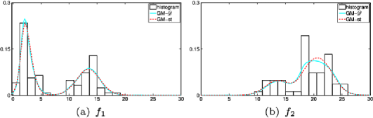
Figure 1: GM–$\mathscr{D}(c,z,P_{0})$ (solid line) vs. GM–st$(\sigma,z,P_{0})$ (dashed line) mixture with random $c$ and $\sigma$, respectively: posterior estimates of the densities $f_{1}$ and $f_{2}$. The displayed histograms are generated by the actual two-sample data.

Our statistical analysis has the following two goals: on the one hand we wish to estimate the densities generating the two samples and, on the other, we aim at obtaining an approximation of the posterior distribution of the number of clusters in each sample. This allows to draw a direct comparison of the inferential outcomes produced by the GM–$\mathscr{D}(c,z,P_{0})$ and GM–st$(\sigma,z,P_{0})$ mixtures. As for the specifications of the hyperparameters in (5) we essentially adopted the quite standard specifications of [10]. Hence, we have set $(w,W)=(1,100)$, $(s,S)=(1,1)$, $(a,A)=((n_{1}\bar{X}+n_{2}\bar{Y})/(n_{1}+n_{2}),2)$ and $(a_{0},b_{0})=(2,1)$ where $\bar{X}$ and $\bar{Y}$ are the sample means for $\mathbf{X}^{(n_{1})}$ and $\mathbf{Y}^{(n_{2})}$, respectively. As for the other parameters involved, we suppose that $c\sim\operatorname{Ga}(2,1)$, whereas $\sigma$ and $z$ are both uniform on $[0,1]$. Moreover, these three parameters are independent. All estimates will be based on $80\mbox{,}000$ iterations of the algorithm after $20\mbox{,}000$ burn-in sweeps.

The estimated densities are displayed in Figure 1 and there seem to be no significant differences. However, regardless the particular mixture model specification, the two species forming each sample are clearly better separated in the first sample. This is not surprising, given that the second sample is formed by two overlapping species. See also the histogram in the background of Figure 1. The results on the clustering structure are reported in Figure 2 and in Table 1. Figure 2 shows that the posterior distributions of the number of clusters corresponding to the GM–st mixture is characterized by a lower variability than in the GM–$\mathscr{D}$ mixture case. Moreover, if one roughly thinks of each species of flowers in a sample as forming a single cluster, then it is apparent that the GM–st mixture better estimates both $K_{\mathbf{X}}$ and $K_{\mathbf{Y}}$. See also Table 1. These results seems to suggest that the parameter $\sigma$, associated to the stable CRM, has a beneficial impact on the estimation of the clustering structure. This is in line with the findings of [23] in the exchangeable case, where it is pointed out that $\sigma$ induces a reinforcement mechanism which improves the capability of learning the clustering structure from the data. We believe this aspect is of great relevance and, hence, deserves further investigation.

Figure 2: GM–$\mathscr{D}(c,z,P_{0})$ (top row) vs. GM–st$(\sigma,z,P_{0})$ (bottom row) mixture with random $c$ and $\sigma$, respectively: posterior distributions of the number of clusters $K_{\mathbf{X}}$ and $K_{\mathbf{Y}}$.

Table 1: GM–$\mathscr{D}(c,z,P_{0})$ vs. GM–st$(\sigma,z,P_{0})$ mixture with random $c$ and $\sigma$, respectively: estimated number of clusters (Col. 1 and 2), maximum a posteriori values ($\hat{K}_{\mathbf{X}}$ and $\hat{K}_{\mathbf{Y}}$) and probability of more than $4$ clusters per sample (Col. 5 and 6)

	$\mathbb{E}[K_{\mathbf{X}}|\ldots]$	$\mathbb{E}[K_{\mathbf{Y}}|\ldots]$	$\hat{K}_{\mathbf{X}}$	$\hat{K}_{\mathbf{Y}}$	$\mathbb{P}(K_{\mathbf{X}}\geq 4)$	$\mathbb{P}(K_{\mathbf{Y}}\geq 4)$
GM–$\mathscr{D}(c,z,P_{0})$	3.72	3.15	3	2	0.50	0.31
GM–st$(\sigma,z,P_{0})$	2.70	2.30	2	2	0.13	0.05

Appendix

.1 Proof of Proposition 1

By combining the definition of GM-dependent normalized CRMs given in (8) with the gamma integral, it is possible to write

$$\mathbb{E}\bigl{[}\tilde{p}_{1}(A)\tilde{p}_{2}(B)\bigr{]}=\int_{0}^{\infty}\int_{0}^{\infty}\mathbb{E}\bigl{[}\mathrm{e}^{-u\tilde{\mu}_{1}(\mathbb{X})-v\tilde{\mu}_{2}(\mathbb{X})}\tilde{\mu}_{1}(A)\tilde{\mu}_{2}(B)\bigr{]}\,\mathrm{d}u\,\mathrm{d}v.$$

Since $\tilde{\mu}_{i}=\mu_{i}+\mu_{0}$ for $i=1,2$, with $\mu_{0}$, $\mu_{1}$ and $\mu_{2}$ independent, one has

$$\mathbb{E}\bigl{[}\mathrm{e}^{-u\mu_{1}(\mathbb{X})-(u+v)\mu_{0}(\mathbb{X})}\mu_{1}(A)\mu_{0}(B)\bigr{]}$$

$$\quad=\mathbb{E}\bigl{[}\mathrm{e}^{-u\mu_{1}(\mathbb{X})}\mu_{1}(A)\bigr{]}\mathbb{E}\bigl{[}\mathrm{e}^{-(u+v)\mu_{0}(\mathbb{X})}\mu_{0}(B)\bigr{]}$$

$$\quad=c^{2}z(1-z)P_{0}(A)P_{0}(B)\mathrm{e}^{-cz\psi(u)-c(1-z)\psi(u+v)}\tau_{1}(u)\tau_{1}(u+v).$$

Use the symbol $A^{i}$ to denote $A$ if $i=1$ and $A^{c}$ if $i=0$. Hence, $\{A^{i}\cap B^{j}\colon\ i,j=0,1\}$ is the partition of $\mathbb{X}$ generated by $\{A,B\}$. Hence,

$$\mathbb{E}\bigl{[}\mathrm{e}^{-(u+v)\mu_{0}(\mathbb{X})}\mu_{0}(A)\mu_{0}(B)\bigr{]}=\sum_{i,j=0}^{1}\mathbb{E}\bigl{[}\mathrm{e}^{-(u+v)\mu_{0}(\mathbb{X})}\mu_{0}\bigl{(}A\cap B^{i}\bigr{)}\mu_{0}\bigl{(}A^{j}\cap B\bigr{)}\bigr{]}.$$

This implies that

$$\mathbb{E}\bigl{[}\mathrm{e}^{-(u+v)\mu_{0}(\mathbb{X})}\mu_{0}(A)\mu_{0}(B)\bigr{]}$$

$$\quad=\mathrm{e}^{-c(1-z)\psi(u+v)}c(1-z)$$

$$\qquad{}\times\Biggl{\{}P_{0}(A\cap B)\tau_{2}(u+v)+c(1-z)\tau_{1}^{2}(u+v)\sum_{i,j=0}^{1}P_{0}\bigl{(}A\cap B^{i}\bigr{)}P_{0}\bigl{(}A^{j}\cap B\bigr{)}\Biggr{\}}$$

$$\quad=\mathrm{e}^{-c(1-z)\psi(u+v)}c(1-z)\bigl{\{}P_{0}(A\cap B)\tau_{2}(u+v)+c(1-z)P_{0}(A)P_{0}(B)\tau_{1}^{2}(u+v)\bigr{\}}.$$

Summing up, it follows that

$$\mathbb{E}\bigl{[}\tilde{p}_{1}(A)\tilde{p}_{2}(B)\bigr{]}$$

$$\quad=\int_{0}^{\infty}\int_{0}^{\infty}\mathrm{e}^{-z(\psi(u)+\psi(v))-c(1-z)\psi(u+v)}$$

$$\hskip 36.0pt\qquad{}\times c\bigl{\{}(1-z)P_{0}(A\cap B)\tau_{2}(u+v)+c^{2}P_{0}(A)P_{0}(B)$$

$$\hskip 56.0pt\qquad{}\times\bigl{[}(1-z)^{2}\tau_{1}^{2}(u+v)+z(1-z)\tau_{1}(u+v)\bigl{(}\tau_{1}(u)+\tau_{1}(v)\bigr{)}$$

$$\hskip 90.0pt{}+z^{2}\tau_{1}(u)\tau_{1}(v)\bigr{]}\bigr{\}}\mathrm{d}u\,\mathrm{d}v.$$

If in the previous expression one sets $A=B=\mathbb{X}$, then the following identity holds true

$$c^{2}\int_{0}^{\infty}\int_{0}^{\infty}\mathrm{e}^{-cz(\psi(u)+\psi(v))-c(1-z)\psi(u+v))}$$

$$\hskip 47.0pt{}\times\bigl{[}(1-z)^{2}\tau_{1}^{2}(u+v)+z(1-z)\tau_{1}(u+v)\bigl{(}\tau_{1}(u)+\tau_{1}(v)\bigr{)}+z^{2}\tau_{1}(u)\tau_{1}(v)\bigr{]}\,\mathrm{d}u\,\mathrm{d}v$$

$$\quad=1-c(1-z)\int_{0}^{\infty}\int_{0}^{\infty}\mathrm{e}^{-c(1-z)\psi(u+v)}\tau_{2}(u+v)\,\mathrm{d}u\,\mathrm{d}v.$$

The results in (1) and in (12) then follows.

.2 Proof of Proposition 2

We first determine the probability distribution of $(\tilde{\pi}_{n_{1},n_{2}},\mathbf{X}^{(n_{1})},\mathbf{Y}^{(n_{2})})$. Here $\tilde{\pi}_{n_{1},n_{2}}$ denotes a random partition of $\{\mathbf{X}^{(n_{1})},\mathbf{Y}^{(n_{2})}\}$ whose generic realization, $\pi_{n_{1},n_{2}}$, splits the $n_{1}+n_{2}$ observations into $\sum_{i=0}^{2}k_{i}$ groups of distinct values with respective frequencies $\{n_{j,1}\}_{j=1}^{k_{1}}$, $\{n_{\ell,1}\}_{\ell=1}^{k_{2}}$ and $\{q_{r,1}+q_{r,2}\}_{r=1}^{k_{0}}$. Henceforth, we shall use the shorter notation

$$\Lambda_{\mathbf{n},\mathbf{k}}(\mathcal{A})=\bigl{(}\tilde{\pi}_{n_{1},n_{2}},\mathbf{X}^{(n_{1})},\mathbf{Y}^{(n_{2})}\bigr{)}^{-1}(\pi_{n_{1},n_{2}},\mathcal{A})$$

with $\mathcal{A}$ standing for the collection of pairwise disjoint sets $\{A_{j,1},A_{\ell,2},A_{r}\colon\ j=1,\ldots,k_{1};\ell=1,\ldots,k_{2};r=1,\ldots,k_{0}\}$. Moreover, for any pair of set function $m_{1}$ and $m_{2}$ on $(\mathbb{X},\mathscr{X})$ we set $\mathbf{m}_{i}^{\mathbf{n}^{(i)}}(\mathcal{A}_{i})=\prod_{j=1}^{k_{i}}m_{i}^{n_{j,i}}(A_{j,i})$ and $(\mathbf{m}_{1}^{\mathbf{q}^{(1)}}\times\mathbf{m}_{2}^{\mathbf{q}^{(2)}})(\mathcal{A}_{0})=\prod_{r=1}^{k_{0}}m_{1}^{q_{r,1}}(A_{r})m_{2}^{q_{r,2}}(A_{r})$. By virtue of (9) one has

$$\mathbb{P}\bigl{[}\Lambda_{\mathbf{n},\mathbf{k}}(\mathcal{A})\bigr{]}=\int_{P_{\mathbb{X}}^{2}}\mathbf{p}_{1}^{\mathbf{n}^{(1)}}(\mathcal{A}_{1})\mathbf{p}_{2}^{\mathbf{n}^{(2)}}(\mathcal{A}_{2})\bigl{(}\mathbf{p}_{1}^{\mathbf{q}^{(1)}}\times\mathbf{p}_{2}^{\mathbf{q}^{(2)}}\bigr{)}(\mathcal{A}_{0})\Phi(\mathrm{d}p_{1},\mathrm{d}p_{2}).$$ (37)

Since each $\tilde{p}_{i}$ is equal, in distribution, to the normalized measure $\tilde{\mu}_{i}/\tilde{\mu}_{i}(\mathbb{X})$ one can proceed in a similar fashion as in the proof of Proposition 1 and write

$$\mathbb{P}\bigl{[}\Lambda_{\mathbf{n},\mathbf{k}}(\mathcal{A})\bigr{]} = \frac{1}{\Gamma(n_{1})\Gamma(n_{2})}\int_{0}^{\infty}\,\mathrm{d}u\int_{0}^{\infty}\,\mathrm{d}v$$

$${}\times\mathbb{E}\bigl{[}\mathrm{e}^{-u\tilde{\mu}_{1}(\mathbb{X})-v\tilde{\mu}_{2}(\mathbb{X})}\tilde{\bolds{\mu}}_{1}^{\mathbf{n}^{(1)}}(\mathcal{A}_{1})\tilde{\bolds{\mu}}_{2}^{\mathbf{n}^{(2)}}(\mathcal{A}_{2})\bigl{(}\tilde{\bolds{\mu}}_{1}^{\mathbf{q}^{(1)}}\times\tilde{\bolds{\mu}}_{2}^{\mathbf{q}^{(2)}}\bigr{)}(\mathcal{A}_{0})\bigr{]}.$$

Since CRMs give rise to mutually independent random variables when evaluated on disjoint sets, which identifies the so-called independence property of CRMs, the expected value in the integral above is shown to coincide with

$$\mathbb{E}\bigl{[}\mathrm{e}^{-u\tilde{\mu}_{1}(\mathbb{X}^{*})-v\tilde{\mu}_{2}(\mathbb{X}^{*})}\bigr{]}\prod_{i=1}^{2}\prod_{j=1}^{k_{i}}\mathbb{E}\bigl{[}\mathrm{e}^{-u\tilde{\mu}_{1}(A_{j,i})-v\tilde{\mu}_{2}(A_{j,i})}\tilde{\mu}_{i}^{n_{j,i}}(A_{j,i})\bigr{]}$$

$$\quad{}\times\prod_{r=1}^{k_{0}}\mathbb{E}\bigl{[}\mathrm{e}^{-u\tilde{\mu}_{1}(A_{r})-v\tilde{\mu}_{2}(A_{r})}\tilde{\mu}_{1}^{q_{r,1}}(A_{r})\tilde{\mu}_{2}^{q_{r,2}}(A_{r})\bigr{]},$$

where $\mathbb{X}^{*}=\mathbb{X}\setminus\{(\bigcup_{i=1}^{2}\bigcup_{j=1}^{k_{i}}A_{j,i})\cup(\bigcup_{r=1}^{k_{0}}A_{r})\}$. In the first product, let us consider $i=1$. A similar line of reasoning holds for $i=2$ as well. If we set $h_{z}(u,v)=z(\psi(u)+\psi(v))+(1-z)\psi(u+v)$, by virtue of the Faà di Bruno formula the $j$th factor coincides with

$$\mathbb{E}\bigl{[}\mathrm{e}^{-u\tilde{\mu}_{1}(A_{j,1})-v\tilde{\mu}_{2}(A_{j,1})}\tilde{\mu}_{1}^{n_{j,1}}(A_{j,1})\bigr{]}$$

$$\quad=(-1)^{n_{j,1}}\frac{\partial^{n_{j,1}}}{\partial u^{n_{j,1}}}\mathrm{e}^{-G(A_{j,1})h_{z}(u,v)}$$

$$\quad=\mathrm{e}^{-G(A_{j,1})h_{z}(u,v)}\bigl{\{}G(A_{j,1})\bigl{(}z\tau_{n_{j,1}}(u)+(1-z)\tau_{n_{j,1}}(v)\bigr{)}+R_{j}(A_{j,1})\bigr{\}},$$

where $R_{j}(A_{j,1})$ is a polynomial in $G(A_{j,1})$ of order greater than $1$ and $G=cP_{0}$. Moreover, a multivariate version of the Faà di Bruno formula, see [5], leads to

$$\mathbb{E}\bigl{[}\mathrm{e}^{-u\tilde{\mu}_{1}(A_{r})-v\tilde{\mu}_{2}(A_{r})}\tilde{\mu}_{1}^{q_{r,1}}(A_{r})\tilde{\mu}_{2}^{q_{r,2}}(A_{r})\bigr{]}$$

$$\quad=(-1)^{q_{r,1}+q_{r,2}}\frac{\partial^{q_{r,1}+q_{r,2}}}{\partial u^{q_{r,1}}\partial v^{q_{r,2}}}\mathrm{e}^{-G(A_{r})h_{z}(u,v)}$$

$$\quad=\mathrm{e}^{-G(A_{r})h_{z}(u,v)}\bigl{\{}G(A_{r})(1-z)\tau_{q_{r,1}+q_{r,2}}(u+v)+R_{r}^{*}(A_{r})\bigr{\}}$$

with $R_{r}^{*}(A_{r})$ denoting a polynomial in $G(A_{r})$ of degree greater than $1$. Combining all these facts together, one obtains

$$\mathbb{P}\bigl{[}\Lambda_{\mathbf{n},\mathbf{k}}(\mathcal{A})\bigr{]}$$

$$\quad=\frac{\prod_{j,\ell,r}G(A_{j,1})G(A_{\ell,2})G(A_{r})}{\Gamma(n_{1})\Gamma(n_{2})}$$

$$\qquad{}\times\sum_{\mathbf{i}\in\{0,1\}^{k_{1}}}\sum_{\mathbf{l}\in\{0,1\}^{k_{2}}}(1-z)^{k_{0}+|\mathbf{i}|+|\mathbf{l}|}z^{k_{1}+k_{2}-|\mathbf{i}|-|\mathbf{l}|}$$

$$\qquad{}\times\int_{0}^{\infty}\int_{0}^{\infty}\prod_{j=1}^{k_{1}}\tau_{n_{j,1}}(u+i_{j}v)\prod_{l=1}^{k_{2}}\tau_{n_{l,2}}(\ell_{l}u+v)\prod_{r=1}^{k_{0}}\tau_{q_{r,1}+q_{r,2}}(u+v)\,\mathrm{d}\,\mathrm{d}v+R_{r}^{**}(\mathcal{A}),$$

where $R_{r}^{**}(\mathcal{A})$ is a polynomial of order greater than $k=k_{1}+k_{2}+k_{0}$ in the variables $G(A_{j,1})$, with $j=1,\ldots,k_{1}$, $G(A_{\ell,2})$, with $\ell=1,\ldots,k_{2}$, and $G(A_{r})$, with $r=1,\ldots,k_{0}$. It is apparent that the probability distribution of $(\mathbf{X}^{(n_{1})},\mathbf{Y}^{(n_{2})})$, conditional on $\tilde{\pi}_{n_{1},n_{2}}=\pi_{n_{1},n_{2}}$, is absolutely continuous with respect to $P_{0}^{k}$ and recall that $P_{0}$ is nonatomic. In order to determine a density of $(\mathbf{X}^{(n_{1})},\mathbf{Y}^{(n_{2})})$, conditional on $\tilde{\pi}_{n_{1},n_{2}}=\pi_{n_{1},n_{2}}$, define $\mathcal{A}_{\varepsilon}$ as the collection of sets $\{A_{j,1}^{\varepsilon},A_{\ell,2}^{\varepsilon},A_{r}^{\varepsilon}:j=1,\ldots,k_{1};\ell=1,\ldots,k_{2};r=1,\ldots,k_{0}\}$ with

$$A_{j,1}^{\varepsilon}\downarrow\{x_{j}\},\qquad A_{\ell,2}^{\varepsilon}\downarrow\{y_{\ell}\},\qquad A_{r}^{\varepsilon}\downarrow\{z_{r}\}$$

as $\varepsilon\downarrow 0$. Hence, a version of the conditional density of $(\mathbf{X}^{(n_{1})},\mathbf{Y}^{(n_{2})})$, conditional on $\tilde{\pi}_{n_{1},n_{2}}=\pi_{n_{1},n_{2}}$, with respect to $P_{0}^{k}$ and evaluated at $(\mathbf{x},\mathbf{y},\mathbf{z})$ is proportional to

$$\lim_{\varepsilon\downarrow 0}\frac{\mathbb{P}[\Lambda_{\mathbf{n},\mathbf{k}}(\mathcal{A}^{\varepsilon})]}{\prod_{j=1}^{k_{1}}P_{0}(A_{j,1}^{\varepsilon})\prod_{\ell=1}^{k_{2}}P_{0}(A_{\ell,2}^{\varepsilon})\prod_{r=1}^{k_{0}}P_{0}(A_{r}^{\varepsilon})}$$

and, from previous expansion, it can be easily seen to coincide with 1. And this proves the statement.

.3 Proof of Proposition 4

The probability distribution $\mathcal{L}^{*}$ defined in (24) can be decomposed as follows

$$\mathcal{L}\bigl{(}\bolds{\theta}^{*},\pi_{n_{1},n_{2}},\bolds{\zeta}\bigr{)}\mathcal{L}\bigl{(}\mathbf{X}^{(n_{1})},\mathbf{Y}^{(n_{2})}|\bolds{\theta}^{*},\pi_{n_{1},n_{2}},\bolds{\zeta}\bigr{)}.$$

In a similar fashion to the proof of Proposition 2, we use the notation

$$\Lambda_{\mathbf{n},\mathbf{k}}(\mathcal{A})=\bigl{(}\tilde{\pi}_{n_{1},n_{2}},\bolds{\theta}^{*}\bigr{)}^{-1}(\pi_{n_{1},n_{2}},\mathcal{A})$$

with $\mathcal{A}$ standing for the collection of pairwise disjoint sets $\{A_{j,1},A_{\ell,2},A_{r}\colon\ j=1,\ldots,k_{1};\ell=1,\ldots,k_{2};r=1,\ldots,k_{0}\}$. By virtue of (9) and by definition of $\bolds{\zeta}=(\bolds\zeta^{(1)},\bolds\zeta^{(2)})$, one has

$$\mathbb{P}\bigl{[}\Lambda_{\mathbf{n},\mathbf{k}}(\mathcal{A})|\bolds\zeta\bigr{]} = \int_{P_{\mathbb{X}}^{3}}\mathbf{p}_{1}^{\mathbf{n}^{(1)}\cdot\bolds\zeta_{1}^{*}}(\mathcal{A}_{1})\mathbf{p}_{2}^{\mathbf{n}^{(2)}\cdot\bolds\zeta_{2}^{*}}(\mathcal{A}_{1})$$

$$\hskip 16.0pt{}\times\mathbf{p}_{0}^{\mathbf{n}^{(1)}\cdot(\mathbf{1}-\bolds\zeta_{1}^{*})}(\mathcal{A}_{1})\mathbf{p}_{0}^{\mathbf{n}^{(2)}\cdot(\mathbf{1}-\bolds\zeta_{2}^{*})}(\mathcal{A}_{2})\mathbf{p}_{0}^{\mathbf{q}^{*}}(\mathcal{A}_{0})\Phi^{\prime}(\mathrm{d}p_{0},\mathrm{d}p_{1},\mathrm{d}p_{2}),$$

where $\Phi^{\prime}$ corresponds to the probability distribution of the random vector

$$\biggl{(}\frac{\mu_{0}}{\mu_{0}(\mathbb{X})},\frac{\mu_{1}}{\mu_{1}(\mathbb{X})},\frac{\mu_{2}}{\mu_{2}(\mathbb{X})}\biggr{)}$$

on $P_{\mathbb{X}}^{3}$ and we have used vector notation to denote the inner products $\mathbf{n}^{(i)}\cdot\bolds{\zeta}_{i}^{*}=\sum_{j=1}^{k_{i}}n_{j,i}\zeta_{j,i}^{*}$ and $\mathbf{n}^{(i)}\cdot(\mathbf{1}-\bolds{\zeta}_{i}^{*})=\sum_{j=1}^{k_{i}}n_{j,i}(1-\zeta_{j,i})$ for $i=1,2$. Moreover, note that

$$\mathbb{P}\bigl{[}\bolds{\zeta}=\bigl{(}\mathbf{a}^{(1)},\mathbf{a}^{(2)}\bigr{)}|\mu_{0},\mu_{1},\mu_{2}\bigr{]}=\frac{\mu_{1}(\mathbb{X})^{|\mathbf{a}^{(1)}|}\mu_{2}(\mathbb{X})^{|\mathbf{a}^{(2)}|/2}\mu_{0}(\mathbb{X})^{n_{1}+n_{2}-|\mathbf{a}^{(1)}|-|\mathbf{a}^{(2)}|/2}}{(\mu_{0}(\mathbb{X})+\mu_{1}(\mathbb{X}))^{n_{1}}(\mu_{0}(\mathbb{X})+\mu_{2}(\mathbb{X}))^{n_{2}}}$$

for any $\mathbf{a}=(\mathbf{a}^{(1)},\mathbf{a}^{(2)})\in\{0,1\}^{n_{1}}\times\{0,2\}^{n_{2}}$. Thus, by similar arguments to those employed in the proofs of Propositions 1 and 2, we can write

$$\mathbb{P}\bigl{[}\Lambda_{\mathbf{n},\mathbf{k}}(\mathcal{A}),\bolds{\zeta}=\mathbf{a}\bigr{]} = \frac{1}{\Gamma(n_{1})\Gamma(n_{2})}\int_{0}^{\infty}\,\mathrm{d}u\int_{0}^{\infty}\,\mathrm{d}vu^{n_{1}-1}v^{n_{2}-1}$$

$$\times{}\mathbb{E}\bigl{[}\mathrm{e}^{-u(\mu_{0}(\mathbb{X})+\mu_{1}(\mathbb{X}))-v(\mu_{0}(\mathbb{X})+\mu_{2}(\mathbb{X}))}\bolds{\mu}_{1}^{\mathbf{n}^{(1)}\cdot\bolds{\zeta}_{1}^{*}}(\mathcal{A}_{1}){\bolds{\mu}}_{0}^{\mathbf{n}^{(1)}\cdot(\mathbf{1}-\bolds{\zeta}_{1}^{*})}(\mathcal{A}_{1})$$

$$\hskip 17.0pt{}\times{\bolds{\mu}}_{2}^{\mathbf{n}^{(2)}\cdot\bolds\zeta_{2}^{*}}(\mathcal{A}_{2}){\bolds{\mu}}_{0}^{\mathbf{n}^{(2)}\cdot(\mathbf{1}-\bolds\zeta_{2}^{*})}(\mathcal{A}_{2})\bigl{(}\bolds{\mu}_{0}^{\mathbf{q}^{*}}\bigr{)}(\mathcal{A}_{0})\bigr{]},$$

where $\mathbf{a}$ is a vector such that $\mathbf{a}^{(i)}$ contains $k_{i}$ labels $\zeta_{j,i}^{*}$ such that

$$\mathbb{P}\bigl{[}\theta_{j,i}^{*}\in A|p_{0},p_{1},p_{2}\bigr{]}=p_{\zeta_{j,i}^{*}}(A).$$

Using the independence property of CRMs and the independence of $\mu_{0}$, $\mu_{1}$ and $\mu_{2}$, the expected value in the integral above can be rewritten as

$$\mathbb{E}\bigl{[}\mathrm{e}^{-u(\mu_{0}(\mathbb{X}^{*})+\mu_{1}(\mathbb{X}^{*}))-v(\mu_{0}(\mathbb{X}^{*})+\mu_{2}(\mathbb{X}^{*}))}\bigr{]}$$

$$\quad\times\prod_{i=1}^{2}\prod_{j=1}^{k_{i}}\mathbb{E}\bigl{[}\mathrm{e}^{-u(\mu_{0}(A_{j,i})+\mu_{1}(A_{j,i}))-v(\mu_{0}(A_{j,i})+\mu_{2}(A_{j,i}))}\mu_{i}(A_{j,i})^{n_{j,i}\zeta_{j,i}^{*}}\mu_{0}(A_{j,i})^{n_{j,i}(1-\zeta_{j,i}^{*})}\bigr{]}$$

$$\quad\times\prod_{r=0}^{k_{0}}\mathbb{E}\bigl{[}\mathrm{e}^{-u(\mu_{0}(A_{r})+\mu_{1}(A_{r}))-v(\mu_{0}(A_{r})+\mu_{2}(A_{r}))}\mu_{0}(A_{r})^{q_{r,1}+q_{r,2}}\bigr{]},$$

where $\mathbb{X}^{*}=\mathbb{X}\setminus\{(\bigcup_{i=1}^{2}\bigcup_{j=1}^{k_{i}}A_{j,i})\cup(\bigcup_{r=1}^{k_{0}}A_{r})\}$. In the first product consider $i=1$, a similar line of reasoning holds then for $i=2$. The $j$th factor coincides with

$$\mathbb{E}\bigl{[}\mathrm{e}^{-v\mu_{2}(A_{j,1})}\bigr{]}\mathbb{E}\bigl{[}\mathrm{e}^{-u\mu_{1}(A_{j,1})}\mu_{1}(A_{j,1})^{n_{j,1}\zeta_{j,1}^{*}}\bigr{]}$$

(39)

$$\quad{}\times\mathbb{E}\bigl{[}\mathrm{e}^{-(u+v)\mu_{0}(A_{j,1})}\mu_{0}(A_{j,1})^{n_{j,1}(1-\zeta_{j,1}^{*})}\bigr{]},$$

where

$$\mathbb{E}\bigl{[}\mathrm{e}^{-v\mu_{2}(A_{j,1})}\bigr{]}=\mathrm{e}^{-cP_{0}(A_{j,1})\psi(v)}$$

and, by virtue of the Faà di Bruno formula,

$$\mathbb{E}\bigl{[}\mathrm{e}^{-u\mu_{1}(A_{j,1})}\mu_{1}(A_{j,1})^{n_{j,1}\zeta_{j,1}^{*}}\bigr{]} = (-1)^{n_{j,1}\zeta_{j,1}^{*}}\frac{\partial^{n_{j,1}\zeta_{j,1}^{*}}}{\partial u^{n_{j,1}\zeta_{j,1}^{*}}}\mathrm{e}^{-czP_{0}(A_{j,1})\psi(u)}$$

$$= \mathrm{e}^{-czP_{0}(A_{j,1})\psi(u)}\bigl{\{}cz\bigl{[}P_{0}(A_{j,1})\tau_{n_{j,1}}(u)+R_{j,1}(A_{j,1})\bigr{]}\bigr{\}}^{\zeta_{j,1}^{*}}$$

and

$$\mathbb{E}\bigl{[}\mathrm{e}^{-(u+v)\mu_{0}(A_{j,1})}\mu_{0}(A_{j,1})^{n_{j,1}(1-\zeta_{j,1}^{*})}\bigr{]}$$

$$\quad=(-1)^{n_{j,1}(1-\zeta_{j,1}^{*})}\frac{\partial^{n_{j,1}(1-\zeta_{j,1}^{*})}}{\partial s^{n_{j,1}(1-\zeta_{j,1}^{*})}}\mathrm{e}^{-c(1-z)P_{0}(A_{j,1})\psi(s)}\Big{|}_{s=u+v}$$

$$\quad=\mathrm{e}^{-c(1-z)P_{0}(A_{j,1})\psi(u+v)}\bigl{\{}c(1-z)\bigl{[}P_{0}(A_{j,1})\tau_{n_{j,1}}(u+v)+R_{j,1}(A_{j,1})\bigr{]}\bigr{\}}^{1-\zeta_{j,1}^{*}}.$$

In the previous expressions, we have agreed that $\partial^{0}/\partial s^{0}$ is the identity operator and that $R_{j,1}(A_{j,1})$ is some polynomial in $P_{0}(A_{j,1})$ of order greater than $1$. Thus, the product in (.3) is equal to

$$\mathrm{e}^{-cP_{0}(A_{j,1})h_{z}(u,v)}cz^{\zeta_{j,1}^{*}}(1-z)^{1-\zeta_{j,1}^{*}}\bigl{\{}P_{0}(A_{j,1})\tau_{n_{j,1}}\bigl{(}u+\bigl{(}1-\zeta_{j,1}^{*}\bigr{)}v\bigr{)}+R_{j,1}(A_{j,1})\bigr{\}}.$$ (40)

Analogously, one has

$$\mathbb{E}\bigl{[}\mathrm{e}^{-u(\mu_{0}(\mathbb{X}^{*})+\mu_{1}(\mathbb{X}^{*}))-v(\mu_{0}(\mathbb{X}^{*})+\mu_{2}(\mathbb{X}^{*}))}\bigr{]}=\mathrm{e}^{-cP_{0}(\mathbb{X}^{*})h_{z}(u,v)}$$ (41)

and

$$\mathbb{E}\bigl{[}\mathrm{e}^{-u(\mu_{0}(A_{r})+\mu_{1}(A_{r}))-v(\mu_{0}(A_{r})+\mu_{2}(A_{r}))}\mu_{0}(A_{r})^{q_{r,1}+q_{r,2}}\bigr{]}$$

(42)

$$\quad=\mathrm{e}^{-cP_{0}(A_{r})h_{z}(u,v)}c(1-z)\bigl{\{}P_{0}(A_{r})\tau_{q_{r,1}+q_{r,2}}(u+v)+R_{r}(A_{r})\bigr{\}},$$

where $R_{r}(A_{r})$ is some polynomial in $P_{0}(A_{r})$ of order greater than $1$. By combining the expressions (40)–(.3), we obtain that $\mathbb{P}[\Lambda_{\mathbf{n},\mathbf{k}}(\mathcal{A}),\bolds{\zeta}=\mathbf{a}]$ coincides with

$$\frac{c^{k}z^{|\bolds{\zeta}_{1}^{*}|+|\bolds{\zeta}_{2}^{*}|}(1-z)^{k_{1}+k_{2}-|\bolds{\zeta}_{1}^{*}|-|\bolds{\zeta}_{2}^{*}|}}{\Gamma(n_{1})\Gamma(n_{2})}P_{0}^{k}(\mathcal{A})$$

$$\quad{}\times\int_{0}^{\infty}\int_{0}^{\infty}u^{n_{1}-1}v^{n_{2}-1}\mathrm{e}^{-ch_{z}(u,v)}\prod_{j=1}^{k_{1}}\tau_{n_{j,1}}\bigl{(}u+\bigl{(}1-\zeta_{j,1}^{*}\bigr{)}v\bigr{)}$$

$$\hskip 38.0pt\qquad{}\times\prod_{j=1}^{k_{2}}\tau_{n_{j,2}}\bigl{(}\bigl{(}1-\zeta_{j,2}^{*}\bigr{)}u+v\bigr{)}\prod_{r=1}^{k_{0}}\tau_{q_{r,1}+q_{r,2}}(u+v)\,\mathrm{d}u\,\mathrm{d}v+R^{*}(\mathcal{A}),$$

where $R^{*}(\mathcal{A})$ is a polynomial in the variables $P_{0}(A_{j,1})$, with $j=1,\ldots,k_{1}$, $P_{0}(A_{\ell,2})$, with $\ell=1,\ldots,k_{2}$, and $P_{0}(A_{r})$, with $r=1,\ldots,k_{0}$, of order greater than $k=k_{1}+k_{2}+k_{0}$ and $P_{0}^{k}(\mathcal{A})=\prod_{i=1}^{k_{1}}\prod_{j=1}^{k_{2}}\prod_{r=1}^{k_{0}}P_{0}(A_{i,1})P_{0}(A_{j,2})P_{0}(A_{r})$. It is apparent that the probability distribution of $(\bolds\theta^{(1)},\bolds\theta^{(2)})$, conditional on $\widetilde{\pi}_{n_{1},n_{2}}=\pi_{n_{1},n_{2}}$, is degenerate on $\Theta^{k}$ and the probability distribution of the distinct values $\bolds{\theta}^{*}=(\bolds{\theta}_{*}^{(1)},\bolds{\theta}_{*}^{(2)},\bolds{\theta}_{*})$ is absolutely continuous with respect to $P_{0}^{k}$. In order to determine a density of $(\bolds\theta^{*},\bolds\zeta^{*},\widetilde{\pi}_{n_{1},n_{2}})$, introduce $\mathcal{A}_{\varepsilon}$ as in the proof of Proposition 2 with

$$A_{j,1}^{\varepsilon}\downarrow\bigl{\{}\theta_{j,1}^{*}\bigr{\}},\qquad A_{\ell,2}^{\varepsilon}\downarrow\bigl{\{}\theta_{\ell,2}^{*}\bigr{\}},\qquad A_{r}^{\varepsilon}\downarrow\bigl{\{}\theta_{r}^{*}\bigr{\}}$$

as $\varepsilon\downarrow 0$ and observe that

$$\lim_{\varepsilon\downarrow 0}\frac{\mathbb{P}[\Lambda_{\mathbf{n},\mathbf{k}}(\mathcal{A}_{\varepsilon})]}{P_{0}^{k}(\mathcal{A}_{\varepsilon})}=g\bigl{(}\mathbf{n}^{(1)},\mathbf{n}^{(2)},\mathbf{q}^{(1)},\mathbf{q}^{(2)},\bolds{\zeta}^{*}\bigr{)}$$

and that

$$\mathcal{L}\bigl{(}\bolds\theta^{*},\bolds\pi_{n_{1},n_{2}},\bolds\zeta\bigr{)}=g\bigl{(}\mathbf{n}^{(1)},\mathbf{n}^{(2)},\mathbf{q}^{(1)},\mathbf{q}^{(2)},\bolds{\zeta}^{*}\bigr{)}\prod_{i=1}^{k}g_{0}\bigl{(}\theta_{i}^{*}\bigr{)}.$$ (43)

Since the vector $(\mathbf{X}^{(n_{1})},\mathbf{Y}^{(n_{2})})$, given the partition $\tilde{\pi}_{n_{1}.n_{2}}=\pi_{n_{1},n_{2}}$ and the distinct values $(\bolds\theta_{*}^{(1)},\bolds\theta_{*}^{(2)},\bolds\theta_{*})$, is independent from the labels $\bolds{\zeta}$, the result follows from (4).

.4 Proof of Corollary 2

If $(\tilde{\mu}_{1},\tilde{\mu}_{2})$ are GM-dependent gamma CRMs, then one has $\tau_{q}=\Gamma(q)(1+u)^{-q}$ and $\psi(u)=\log(1+u).$ By plugging these expressions into (4) and resorting to identity 3.197.1 in [14], we obtain that $g(\mathbf{n}^{(1)},\mathbf{n}^{(2)},\mathbf{q}^{(1)},\mathbf{q}^{(2)},\bolds{\zeta}^{*})$ is equal to

$$c^{k}z^{\tilde{k}_{1}+\tilde{k}_{2}}(1-z)^{\tilde{k}_{0}}\frac{\Gamma(c+n_{1}-\bar{n}_{1})}{\Gamma(n_{1})\Gamma(c+n_{1}+n_{2}-\bar{n}_{1})}\xi\bigl{(}\mathbf{n}^{(1)},\mathbf{n}^{(2)},\mathbf{q}^{*}\bigr{)}$$

(44)

$$\quad{}\times\int_{0}^{\infty}u^{n_{1}-1}(1+u)^{-c-n_{1}+\bar{n}_{2}}{}_{2}F_{1}(\bar{n}_{2}+cz,n_{2};n_{1}+n_{2}-\bar{n}_{1}+c;-u)\,\mathrm{d}u,$$

where we recall that $\tilde{k}_{0}=k_{1}+k_{2}-\tilde{k}_{1}-\tilde{k}_{2}$. The simple change of variable $t=u/(1+u)$ and the transformation formula for hypergeometric functions

$${}_{2}F_{1}(\alpha,\beta;\gamma;z)=(1-z)^{-\alpha}{}_{2}F_{1}\bigl{(}\alpha,\gamma-\beta;\gamma;z/(z-1)\bigr{)}$$

let us rewrite the integral in (.4) as

$$\int_{0}^{1}t^{n_{1}-1}(1-t)^{c+cz-1}{}_{2}F_{1}(\bar{n}_{2}+cz,c+n_{1}-\bar{n}_{1};c+n_{1}+n_{2}-\bar{n}_{1};t)\,\mathrm{d}t.$$

The proof is then completed by resorting to identity 7.512.5 in [14].

.5 Proof of Corollary 3

If $(\tilde{\mu}_{1},\tilde{\mu}_{2})$ are GM-dependent $\sigma$-stable CRMs, then one has $\tau_{q}=\sigma(1-\sigma)_{q-1}u^{\sigma-q}$ and $\psi(u)=u^{\sigma}.$ By plugging these expressions into (4) we obtain that $g(\mathbf{n}^{(1)},\mathbf{n}^{(2)},\mathbf{q}^{(1)},\mathbf{q}^{(2)},\bolds{\zeta}^{*})$ is equal to

$$\frac{c^{k}z^{\tilde{k}_{1}+\tilde{k}_{2}}(1-z)^{\tilde{k}_{0}}\sigma^{k}}{\Gamma(n_{1})\Gamma(n_{2})}\xi_{\sigma}\bigl{(}\mathbf{n}^{(n_{1})},\mathbf{n}^{(n_{2})},\mathbf{q}^{*}\bigr{)}$$

$$\quad{}\times\int_{0}^{\infty}\int_{0}^{\infty}\frac{u^{n_{1}-\bar{n}_{1}+\tilde{k}_{1}\sigma-1}v^{n_{2}-\bar{n}_{2}+\tilde{k}_{2}\sigma-1}(u+v)^{\tilde{k}_{0}\sigma-n_{1}-n_{2}+\bar{n}_{1}+\bar{n}_{2}}}{\exp\{c[z(u^{\sigma}+v^{\sigma})+(1-z)(u+v)^{\sigma}]\}}\,\mathrm{d}u\,\mathrm{d}v.$$

The proof is completed by carefully applying the change of variables $w=u/(u+v)$ and $s=u+v$.

References

• [1] {barticle}[mr] \bauthor\bsnmAntoniak, \bfnmCharles E.\binitsC.E. (\byear1974). \btitleMixtures of Dirichlet processes with applications to Bayesian nonparametric problems. \bjournalAnn. Statist. \bvolume2 \bpages1152–1174. \bidissn=0090-5364, mr=0365969 \bptokimsref \endbibitem
• [2] {bbook}[mr] \bauthor\bsnmBailey, \bfnmW. N.\binitsW.N. (\byear1964). \btitleGeneralized Hypergeometric Series. \bseriesCambridge Tracts in Mathematics and Mathematical Physics, No. 32. \blocationNew York: \bpublisherStechert-Hafner, Inc. \bidmr=0185155 \bptokimsref \endbibitem
• [3] {barticle}[mr] \bauthor\bsnmBarrientos, \bfnmAndrés F.\binitsA.F., \bauthor\bsnmJara, \bfnmAlejandro\binitsA. &\bauthor\bsnmQuintana, \bfnmFernando A.\binitsF.A. (\byear2012). \btitleOn the support of MacEachern’s dependent Dirichlet processes and extensions. \bjournalBayesian Anal. \bvolume7 \bpages277–309. \biddoi=10.1214/12-BA709, issn=1936-0975, mr=2934952 \bptokimsref \endbibitem
• [4] {bmisc}[auto:STB—2013/05/29—08:31:43] \bauthor\bsnmCifarelli, \bfnmD. M.\binitsD.M. &\bauthor\bsnmRegazzini, \bfnmE.\binitsE. (\byear1978). \bhowpublishedProblemi statistici non parametrici in condizioni di scambiabilità parziale. Quaderni Istituto Matematica Finanziaria, Università di Torino Serie III, 12. English translation. Available at: http://www.unibocconi.it/wps/allegatiCTP/CR-Scamb-parz[1].20080528.135739.pdf. \bptokimsref \endbibitem
• [5] {barticle}[mr] \bauthor\bsnmConstantine, \bfnmG. M.\binitsG.M. &\bauthor\bsnmSavits, \bfnmT. H.\binitsT.H. (\byear1996). \btitleA multivariate Faà di Bruno formula with applications. \bjournalTrans. Amer. Math. Soc. \bvolume348 \bpages503–520. \biddoi=10.1090/S0002-9947-96-01501-2, issn=0002-9947, mr=1325915 \bptokimsref \endbibitem
• [6] {bbook}[mr] \bauthor\bsnmDaley, \bfnmD. J.\binitsD.J. &\bauthor\bsnmVere-Jones, \bfnmD.\binitsD. (\byear1988). \btitleAn Introduction to the Theory of Point Processes. \bseriesSpringer Series in Statistics. \blocationNew York: \bpublisherSpringer. \bidmr=0950166 \bptokimsref \endbibitem
• [7] {bincollection}[auto:STB—2013/05/29—08:31:43] \bauthor\bparticlede \bsnmFinetti, \bfnmB.\binitsB. (\byear1938). \btitleSur la condition d’equivalence partielle. In \bbooktitleActualités Scientifiques et Industrielles, \bvolume739 \bpages5–18. \blocationParis: \bpublisherHerman. \bptokimsref \endbibitem
• [8] {bincollection}[mr] \bauthor\bsnmDunson, \bfnmDavid B.\binitsD.B. (\byear2010). \btitleNonparametric Bayes applications to biostatistics. In \bbooktitleBayesian Nonparametrics (\beditor\binitsN.L.\bfnmN. L. \bsnmHjort, \beditor\binitsC.C.\bfnmC. C. \bsnmHolmes, \beditor\binitsP.\bfnmP. \bsnmMüller &\beditor\binitsS.G.\bfnmS. G. \bsnmWalker, eds.). \bseriesCamb. Ser. Stat. Probab. Math. \bpages223–273. \blocationCambridge: \bpublisherCambridge Univ. Press. \bidmr=2730665 \bptokimsref \endbibitem
• [9] {barticle}[mr] \bauthor\bsnmEpifani, \bfnmIlenia\binitsI. &\bauthor\bsnmLijoi, \bfnmAntonio\binitsA. (\byear2010). \btitleNonparametric priors for vectors of survival functions. \bjournalStatist. Sinica \bvolume20 \bpages1455–1484. \bidissn=1017-0405, mr=2777332 \bptokimsref \endbibitem
• [10] {barticle}[mr] \bauthor\bsnmEscobar, \bfnmMichael D.\binitsM.D. &\bauthor\bsnmWest, \bfnmMike\binitsM. (\byear1995). \btitleBayesian density estimation and inference using mixtures. \bjournalJ. Amer. Statist. Assoc. \bvolume90 \bpages577–588. \bidissn=0162-1459, mr=1340510 \bptokimsref \endbibitem
• [11] {barticle}[mr] \bauthor\bsnmEwens, \bfnmW. J.\binitsW.J. (\byear1972). \btitleThe sampling theory of selectively neutral alleles. \bjournalTheoret. Population Biology \bvolume3 \bpages87–112. \bidissn=0040-5809, mr=0325177 \bptnotecheck related\bptokimsref \endbibitem
• [12] {barticle}[mr] \bauthor\bsnmFerguson, \bfnmThomas S.\binitsT.S. (\byear1973). \btitleA Bayesian analysis of some nonparametric problems. \bjournalAnn. Statist. \bvolume1 \bpages209–230. \bidissn=0090-5364, mr=0350949 \bptokimsref \endbibitem
• [13] {barticle}[mr] \bauthor\bsnmGelfand, \bfnmAlan E.\binitsA.E. &\bauthor\bsnmKottas, \bfnmAthanasios\binitsA. (\byear2002). \btitleA computational approach for full nonparametric Bayesian inference under Dirichlet process mixture models. \bjournalJ. Comput. Graph. Statist. \bvolume11 \bpages289–305. \biddoi=10.1198/106186002760180518, issn=1061-8600, mr=1938136 \bptokimsref \endbibitem
• [14] {bbook}[mr] \bauthor\bsnmGradshteyn, \bfnmI. S.\binitsI.S. &\bauthor\bsnmRyzhik, \bfnmI. M.\binitsI.M. (\byear2007). \btitleTable of Integrals, Series, and Products, \bedition7th ed. \blocationAmsterdam: \bpublisherElsevier/Academic Press. \bidmr=2360010 \bptokimsref \endbibitem
• [15] {barticle}[mr] \bauthor\bsnmGriffiths, \bfnmR. C.\binitsR.C. &\bauthor\bsnmMilne, \bfnmR. K.\binitsR.K. (\byear1978). \btitleA class of bivariate Poisson processes. \bjournalJ. Multivariate Anal. \bvolume8 \bpages380–395. \biddoi=10.1016/0047-259X(78)90061-1, issn=0047-259X, mr=0512608 \bptokimsref \endbibitem
• [16] {barticle}[mr] \bauthor\bsnmIshwaran, \bfnmHemant\binitsH. &\bauthor\bsnmJames, \bfnmLancelot F.\binitsL.F. (\byear2001). \btitleGibbs sampling methods for stick-breaking priors. \bjournalJ. Amer. Statist. Assoc. \bvolume96 \bpages161–173. \biddoi=10.1198/016214501750332758, issn=0162-1459, mr=1952729 \bptokimsref \endbibitem
• [17] {barticle}[mr] \bauthor\bsnmJames, \bfnmLancelot F.\binitsL.F. (\byear2005). \btitleBayesian Poisson process partition calculus with an application to Bayesian Lévy moving averages. \bjournalAnn. Statist. \bvolume33 \bpages1771–1799. \biddoi=10.1214/009053605000000336, issn=0090-5364, mr=2166562 \bptokimsref \endbibitem
• [18] {barticle}[mr] \bauthor\bsnmJames, \bfnmLancelot F.\binitsL.F., \bauthor\bsnmLijoi, \bfnmAntonio\binitsA. &\bauthor\bsnmPrünster, \bfnmIgor\binitsI. (\byear2006). \btitleConjugacy as a distinctive feature of the Dirichlet process. \bjournalScand. J. Stat. \bvolume33 \bpages105–120. \biddoi=10.1111/j.1467-9469.2005.00486.x, issn=0303-6898, mr=2255112 \bptokimsref \endbibitem
• [19] {barticle}[mr] \bauthor\bsnmJames, \bfnmLancelot F.\binitsL.F., \bauthor\bsnmLijoi, \bfnmAntonio\binitsA. &\bauthor\bsnmPrünster, \bfnmIgor\binitsI. (\byear2009). \btitlePosterior analysis for normalized random measures with independent increments. \bjournalScand. J. Stat. \bvolume36 \bpages76–97. \biddoi=10.1111/j.1467-9469.2008.00609.x, issn=0303-6898, mr=2508332 \bptokimsref \endbibitem
• [20] {bbook}[mr] \bauthor\bsnmKingman, \bfnmJ. F. C.\binitsJ.F.C. (\byear1993). \btitlePoisson Processes. \bseriesOxford Studies in Probability \bvolume3. \blocationNew York: \bpublisherThe Clarendon Press Oxford Univ. Press. \bidmr=1207584 \bptokimsref \endbibitem
• [21] {barticle}[auto] \bauthor\bsnmKolossiatis, \bfnmM.\binitsM., \bauthor\bsnmGriffin, \bfnmJ. E.\binitsJ.E. &\bauthor\bsnmSteel, \bfnmM. F. J.\binitsM.F.J. (\byear2013). \btitleOn Byesian nonparametric modelling of two correlated distributions. \bjournalStatistics and Computing \bvolume23 \bpages1–15. \bptokimsref \endbibitem
• [22] {barticle}[mr] \bauthor\bsnmLeisen, \bfnmFabrizio\binitsF. &\bauthor\bsnmLijoi, \bfnmAntonio\binitsA. (\byear2011). \btitleVectors of two-parameter Poisson–Dirichlet processes. \bjournalJ. Multivariate Anal. \bvolume102 \bpages482–495. \biddoi=10.1016/j.jmva.2010.10.008, issn=0047-259X, mr=2755010 \bptokimsref \endbibitem
• [23] {barticle}[mr] \bauthor\bsnmLijoi, \bfnmAntonio\binitsA., \bauthor\bsnmMena, \bfnmRamsés H.\binitsR.H. &\bauthor\bsnmPrünster, \bfnmIgor\binitsI. (\byear2007). \btitleControlling the reinforcement in Bayesian non-parametric mixture models. \bjournalJ. R. Stat. Soc. Ser. B Stat. Methodol. \bvolume69 \bpages715–740. \biddoi=10.1111/j.1467-9868.2007.00609.x, issn=1369-7412, mr=2370077 \bptokimsref \endbibitem
• [24] {bincollection}[mr] \bauthor\bsnmLijoi, \bfnmAntonio\binitsA. &\bauthor\bsnmPrünster, \bfnmIgor\binitsI. (\byear2010). \btitleModels beyond the Dirichlet process. In \bbooktitleBayesian Nonparametrics (\beditor\binitsN.L.\bfnmN. L. \bsnmHjort, \beditor\binitsC.C.\bfnmC. C. \bsnmHolmes, \beditor\binitsP.\bfnmP. \bsnmMüller &\beditor\binitsS.G.\bfnmS. G. \bsnmWalker, eds.). \bseriesCamb. Ser. Stat. Probab. Math. \bpages80–136. \blocationCambridge: \bpublisherCambridge Univ. Press. \bidmr=2730661 \bptokimsref \endbibitem
• [25] {barticle}[mr] \bauthor\bsnmMacEachern, \bfnmSteven N.\binitsS.N. (\byear1994). \btitleEstimating normal means with a conjugate style Dirichlet process prior. \bjournalComm. Statist. Simulation Comput. \bvolume23 \bpages727–741. \biddoi=10.1080/03610919408813196, issn=0361-0918, mr=1293996 \bptokimsref \endbibitem
• [26] {bincollection}[auto:STB—2013/05/29—08:31:43] \bauthor\bsnmMacEachern, \bfnmS. N.\binitsS.N. (\byear1999). \btitleDependent nonparametric processes. In \bbooktitleASA Proceedings of the Section on Bayesian Statistical Science \blocationAlexandria, VA: \bpublisherAmerican Statistical Association. \bptokimsref \endbibitem
• [27] {bmisc}[auto:STB—2013/05/29—08:31:43] \bauthor\bsnmMacEachern, \bfnmS. N.\binitsS.N. (\byear2000). \bhowpublishedDependent Dirichlet processes. Technical report, Ohio State Univ. \bptokimsref \endbibitem
• [28] {barticle}[mr] \bauthor\bsnmMüller, \bfnmPeter\binitsP., \bauthor\bsnmQuintana, \bfnmFernando\binitsF. &\bauthor\bsnmRosner, \bfnmGary\binitsG. (\byear2004). \btitleA method for combining inference across related nonparametric Bayesian models. \bjournalJ. R. Stat. Soc. Ser. B Stat. Methodol. \bvolume66 \bpages735–749. \biddoi=10.1111/j.1467-9868.2004.05564.x, issn=1369-7412, mr=2088779 \bptokimsref \endbibitem
• [29] {barticle}[mr] \bauthor\bsnmMüller, \bfnmPeter\binitsP. &\bauthor\bsnmQuintana, \bfnmFernando A.\binitsF.A. (\byear2004). \btitleNonparametric Bayesian data analysis. \bjournalStatist. Sci. \bvolume19 \bpages95–110. \biddoi=10.1214/088342304000000017, issn=0883-4237, mr=2082149 \bptokimsref \endbibitem
• [30] {bmisc}[auto:STB—2013/05/29—08:31:43] \bauthor\bsnmNipoti, \bfnmB.\binitsB. (\byear2011). \bhowpublishedDependent completely random measures and statistical applications. Ph.D. thesis, Dept. Mathematics, Univ. Pavia. \bptokimsref \endbibitem
• [31] {barticle}[mr] \bauthor\bsnmOlkin, \bfnmIngram\binitsI. &\bauthor\bsnmLiu, \bfnmRuixue\binitsR. (\byear2003). \btitleA bivariate beta distribution. \bjournalStatist. Probab. Lett. \bvolume62 \bpages407–412. \biddoi=10.1016/S0167-7152(03)00048-8, issn=0167-7152, mr=1973316 \bptokimsref \endbibitem
• [32] {barticle}[mr] \bauthor\bsnmOrbanz, \bfnmPeter\binitsP. (\byear2011). \btitleProjective limit random probabilities on Polish spaces. \bjournalElectron. J. Stat. \bvolume5 \bpages1354–1373. \biddoi=10.1214/11-EJS641, issn=1935-7524, mr=2842908 \bptokimsref \endbibitem
• [33] {bbook}[mr] \bauthor\bsnmPitman, \bfnmJ.\binitsJ. (\byear2006). \btitleCombinatorial Stochastic Processes. \bseriesLecture Notes in Math. \bvolume1875. \blocationBerlin: \bpublisherSpringer. \bidmr=2245368 \bptokimsref \endbibitem
• [34] {bmisc}[auto:STB—2013/05/29—08:31:43] \bauthor\bsnmPrünster, \bfnmI.\binitsI. (\byear2002). \bhowpublishedRandom probability measures derived from increasing additive processes and their application to Bayesian statistics. Ph.D thesis, Univ. Pavia. \bptokimsref \endbibitem
• [35] {bmisc}[auto:STB—2013/05/29—08:31:43] \bauthor\bsnmRao, \bfnmV. A.\binitsV.A. &\bauthor\bsnmTeh, \bfnmY. W.\binitsY.W. (\byear2009). \bhowpublishedSpatial normalized Gamma processes. In Advances in Neural Information Processing Systems 22. NIPS Foundation. Available at http://books.nips.cc/papers/files/nips22/NIPS2009_0744.pdf. \bptokimsref \endbibitem
• [36] {barticle}[mr] \bauthor\bsnmRegazzini, \bfnmEugenio\binitsE., \bauthor\bsnmLijoi, \bfnmAntonio\binitsA. &\bauthor\bsnmPrünster, \bfnmIgor\binitsI. (\byear2003). \btitleDistributional results for means of normalized random measures with independent increments. \bjournalAnn. Statist. \bvolume31 \bpages560–585. \biddoi=10.1214/aos/1051027881, issn=0090-5364, mr=1983542 \bptokimsref \endbibitem
• [37] {bincollection}[mr] \bauthor\bsnmTeh, \bfnmYee Whye\binitsY.W. &\bauthor\bsnmJordan, \bfnmMichael I.\binitsM.I. (\byear2010). \btitleHierarchical Bayesian nonparametric models with applications. In \bbooktitleBayesian Nonparametrics (\beditor\binitsN.L.\bfnmN. L. \bsnmHjort, \beditor\binitsC.C.\bfnmC. C. \bsnmHolmes, \beditor\binitsP.\bfnmP. \bsnmMüller &\beditor\binitsS.G.\bfnmS. G. \bsnmWalker, eds.). \bseriesCamb. Ser. Stat. Probab. Math. \bpages158–207. \blocationCambridge: \bpublisherCambridge Univ. Press. \bidmr=2730663 \bptokimsref \endbibitem
• [38] {bincollection}[mr] \bauthor\bsnmWest, \bfnmMike\binitsM., \bauthor\bsnmMüller, \bfnmPeter\binitsP. &\bauthor\bsnmEscobar, \bfnmMichael D.\binitsM.D. (\byear1994). \btitleHierarchical priors and mixture models, with application in regression and density estimation. In \bbooktitleAspects of Uncertainty. \bseriesWiley Ser. Probab. Math. Statist. Probab. Math. Statist. \bpages363–386. \blocationChichester: \bpublisherWiley. \bidmr=1309702 \bptokimsref \endbibitem