A Variational Approach to Enhanced Sampling and Free Energy Calculations

Abstract

The ability of widely used sampling methods, such as molecular dynamics or Monte Carlo, to explore complex free energy landscapes is severely hampered by the presence of kinetic bottlenecks. A large number of solutions have been proposed to alleviate this problem. Many are based on the introduction of a bias potential which is a function of a small number of collective variable. However constructing such a bias is not simple. Here we introduce a functional of the bias potential and an associated variational principle. The bias that minimizes the functional relates in a simple way to the free energy surface. This variational principle can be turned into a practical, efficient and flexible sampling method. A number of numerical examples are presented which include the determination of a three dimensional free energy surface. We argue that, beside being numerically advantageous, our variational approach provides a convenient standpoint for looking with novel eyes at the sampling problem.

Molecular Dynamics (MD) and Monte Carlo (MC) simulations have become indispensable tools in many areas of science. However, whenever there are kinetic bottlenecks that lead to the appearance of long-lived metastable states, the computational cost of sampling the systems configuration space becomes prohibitive. This has lead to an intensive search for enhanced methods capable of lifting this severe limitation. One of the oldest such methods and still much in use today is umbrella sampling Torrie and Valleau (1977) in which an external bias is added to the system to favor transitions between states separated by kinetic barriers and allows them to occur on the time scale of the simulation. However building such potential is very challenging and many methods have been devised to this effect  Huber et al. (1994); Darve and Pohorille (2001); Wang and Landau (2001); Laio and Parrinello (2002); Hansmann and Wille (2002); Maragliano and Vanden-Eijnden (2006); Abrams and Vanden-Eijnden (2010); Maragakis et al. (2009).

Here we present a new and efficient approach to this problem and propose a variational method that allows constructing an effective bias potential and leads to an accurate determination of the free energy as a function of a set of chosen collective variables (CVs).

In the following we consider a system described by the microscopic coordinates $\mathbf{R}\in\mathbb{R}^{3N}$ whose dynamics (e.g. MD or MC) at temperature $T$ evolves according to a potential energy function $U(\mathbf{R})$, and leads to a canonical equilibrium distribution $P(\mathbf{R})=e^{-\beta U(\mathbf{R})}/Z$ where $\beta=(k_{\mathrm{B}}T)^{-1}$ is the inverse temperature and $Z=\int d\mathbf{R}\,e^{-\beta U(\mathbf{R})}$ is the partition function of the system. We map the high dimensional $\mathbf{R}$ space into a much smaller and smoother $d$ dimensional space by introducing the set of collective variables $\mathbf{s}(\mathbf{R})=\left(s_{1}(\mathbf{R}),s_{2}(\mathbf{R}),\ldots,s_{d}(\mathbf{R})\right)$ that give a coarse grained but physically cogent description of the system. The appropriate choice of these collective variables is much discussed in the literature Barducci et al. (2011) and here we assume that their selection has been wise. The free energy surface (FES) associated to the CV set $\mathbf{s}$ is defined up to constant as

$$F(\mathbf{s})=-\frac{1}{\beta}\log\int d\mathbf{R}\,\delta(\mathbf{s}-\mathbf{s}(\mathbf{R}))e^{-\beta U(\mathbf{R})}.$$ (1)

The corresponding equilibrium distribution is $P(\mathbf{s})=e^{-\beta F(\mathbf{s})}/Z$ and the partition function can be rewritten as $Z=\int d\mathbf{s}\,e^{-\beta F(\mathbf{s})}$.

We introduce now the following functional of a bias potential $V(\mathbf{s})$

$$\Omega[V] =\frac{1}{\beta}\log\frac{\int d\mathbf{s}\,e^{-\beta\left[F(\mathbf{s})+V(\mathbf{s})\right]}}{\int d\mathbf{s}\,e^{-\beta F(\mathbf{s})}}+\int d\mathbf{s}\,p(\mathbf{s})V(\mathbf{s})$$ (2)

where $p(\mathbf{s})$ is arbitrary probability distribution that is assumed to be normalized. The second term can thus be read as the expectation value of $V(\mathbf{s})$ over the distribution $p(\mathbf{s})$. As shown in the Supplemental Material (SM), this functional is convex and invariant under the addition of an arbitrary constant to $V(\mathbf{s})$, $\Omega[V+k]=\Omega[V]$ .

The potential that renders $\Omega[V]$ stationary is, within an irrelevant constant,

$$V(\mathbf{s})=-F(\mathbf{s})-{\frac{1}{\beta}}\log{p(\mathbf{s})}$$ (3)

for $p(\mathbf{s})\neq 0$ and $V(\mathbf{s})=\infty$ otherwise. This stationary point is also the global minimum of $\Omega[V]$ since the functional is convex. When the optimal bias potential (Eq. 3) acts on the system the $\mathbf{s}$ values sampled will be only those for which $p(\mathbf{s})\neq 0$ and $p(\mathbf{s})$ will be their resulting distribution. This offers the interesting possibility of selecting the region in CV space to be explored by appropriately choosing $p(\mathbf{s})$ (see below and SM). In more general terms the freedom of choosing $p(\mathbf{s})$ confers a high degree of flexibility to the method.

If the CVs are defined in a compact phase space of volume $\Omega_{\mathbf{s}}$ a one possible and perhaps natural choice is to take $p(\mathbf{s})=\frac{1}{\Omega_{\mathbf{s}}}$ which leads to a uniform sampling in CV space as commonly done in other enhanced sampling approaches. In this case $V(\mathbf{s})=-F(\mathbf{s})$ modulo a constant which is the same relation as is obeyed in the asymptotic limit by the bias potential in standard metadynamics Laio and Parrinello (2002). If the CVs are unbound then $p(\mathbf{s})$ can be employed to focus on the range of $\mathbf{s}$ to be explored. Another possibility is to use as $p(\mathbf{s})$

$$p(\mathbf{s})=\frac{e^{-\beta^{\prime}F(\mathbf{s})}}{\int d\mathbf{s}\,e^{-\beta^{\prime}F(\mathbf{s})}}$$ (4)

where $\beta^{\prime}=(k_{\mathrm{B}}(T+\Delta T))^{-1}$ and $F(\mathbf{s})$ is our target free energy surface at inverse temperature $\beta$ as defined in Eq. 1 above. This is the distribution sampled in well-tempered metadynamics with a bias factor $\gamma=\frac{\beta}{\beta^{\prime}}$ Barducci et al. (2008). With this choice the relation between the bias potential and free energy becomes identical to the one that asymptotically holds in well-tempered metadynamics Barducci et al. (2008); Dama et al. (2014), $V(\mathbf{s})=-(1-\frac{1}{\gamma})F(\mathbf{s})$. We shall defer to a future publication the exploration of this intriguing possibility. Finally we note that it is our belief that an appropriate choice of $p(\mathbf{s})$ and smart usage of the variational flexibility of the bias potential can be of great help when considering difficult multidimensional CV spaces. We intend to explore this further in the future.

To make use of the variational property of $\Omega[V]$ we write the bias potential $V(\mathbf{s};\boldsymbol{\alpha})$ as a function of the set of variational parameters $\boldsymbol{\alpha}=\left(\alpha_{1},\alpha_{2},\ldots,\alpha_{K}\right)$ and then minimize the function $\Omega(\boldsymbol{\alpha})=\Omega[V(\boldsymbol{\alpha})]$ with respect to $\boldsymbol{\alpha}$. Of course the search for the minimum will be greatly facilitated by the convexity of the functional. From the converged potential $V(\mathbf{s};\boldsymbol{\alpha})$ we can then estimate $F(\mathbf{s})$ directly from Eq. 3 if the assumed functional form has enough variational flexibility. Otherwise, we can always estimate the FES as a function of $\mathbf{s}$, or some other CVs, by employing the standard umbrella sampling relation

$$P(\mathbf{R})\propto e^{\beta V(\mathbf{s}(\mathbf{R}))}P_{V}(\mathbf{R})$$ (5)

where $P_{V}(\mathbf{R})$ is the distribution biased by $V(\mathbf{s}(\mathbf{R}))$ (see the SM for further discussion on this equation). The reweighting can also be performed before the potential has fully converged or even on the fly during the optimisation if the biasing potential converges quickly to a quasi-stationary state during the optimisation process.

In order to implement the optimisation procedure, we shall need to estimate the gradient $\Omega^{\prime}(\boldsymbol{\alpha})$,

$$\frac{\partial\Omega(\boldsymbol{\alpha})}{\partial\alpha_{i}}=-\left<\frac{\partial V(\mathbf{s};\boldsymbol{\alpha})}{\partial\alpha_{i}}\right>_{V(\boldsymbol{\alpha})}+\left<\frac{\partial V(\mathbf{s};\boldsymbol{\alpha})}{\partial\alpha_{i}}\right>_{p},$$ (6)

and the Hessian $\Omega^{\prime\prime}(\boldsymbol{\alpha})$,

$$\frac{\partial^{2}\Omega(\boldsymbol{\alpha})}{\partial\alpha_{j}\partial\alpha_{i}} =\beta\cdot\mathrm{Cov}\left[\frac{\partial V(\mathbf{s};\boldsymbol{\alpha})}{\partial\alpha_{j}},\frac{\partial V(\mathbf{s};\boldsymbol{\alpha})}{\partial\alpha_{i}}\right]_{V(\boldsymbol{\alpha})}$$

$$-\left<\frac{\partial^{2}V(\mathbf{s};\boldsymbol{\alpha})}{\partial\alpha_{j}\partial\alpha_{i}}\right>_{V(\boldsymbol{\alpha})}+\left<\frac{\partial^{2}V(\mathbf{s};\boldsymbol{\alpha})}{\partial\alpha_{j}\partial\alpha_{i}}\right>_{p},$$ (7)

where $\left<\cdots\right>_{V(\boldsymbol{\alpha})}$ and $\mathrm{Cov}[\cdots]_{V(\boldsymbol{\alpha})}$ are the the expectation value and the covariance, respectively, obtained in a biased simulation employing the potential $V(\mathbf{s};\boldsymbol{\alpha})$ and $\left<\cdots\right>_{p}$ is an expectation value in the distribution $p(\mathbf{s})$. A natural approach is to expand $V(\mathbf{s};\boldsymbol{\alpha})$ in a linear basis set and use the coefficient of this expansion as variational parameters

$$V(\mathbf{s};\boldsymbol{\alpha})=\sum_{\mathbf{k}}\alpha_{\mathbf{k}}\cdot G_{\mathbf{k}}(\mathbf{s}),$$ (8)

Given the fact that in general the FES is a rather smooth function of the CVs a small number of terms in this expansion will usually suffice. This is to be contrasted with metadynamics where a large number of Gaussians are used to represent $V(\mathbf{s})$. As we shall see below this leads to great efficiency. In this case the gradient and the Hessian simplify

$$\frac{\partial\Omega(\boldsymbol{\alpha})}{\partial\alpha_{\mathbf{i}}}=-\left<G_{\mathbf{i}}(\mathbf{s})\right>_{V(\boldsymbol{\alpha})}+\left<G_{\mathbf{i}}(\mathbf{s})\right>_{p},$$ (9)

$$\frac{\partial^{2}\Omega(\boldsymbol{\alpha})}{\partial\alpha_{\mathbf{j}}\partial\alpha_{\mathbf{i}}}=\beta\cdot\mathrm{Cov}\left[G_{\mathbf{j}}(\mathbf{s}),G_{\mathbf{i}}(\mathbf{s})\right]_{V(\boldsymbol{\alpha})}.$$ (10)

The gradient and Hessian terms for the constant term $\alpha_{\mathbf{0}}$ are zero for any given $p(\mathbf{s})$ so we can naturally take the constant term as zero and drop it from the linear expansion.

Since the gradients and the Hessian are computed statistically they are intrinsically noisy and one would need very long sampling times if we were to use them in conventional deterministic optimisation algorithms. Thus we turn to the vast literature on stochastic optimization methods Kushner and Yin (2003) and use a recent stochastic gradient descent based algorithm Bach and Moulines (2013). In this algorithm, we consider at iteration $n$ both the instantaneous iterate $\boldsymbol{\alpha}^{(n)}$ and the averaged iterates $\bar{\boldsymbol{\alpha}}^{(n)}=(n+1)^{-1}\sum_{k=0}^{n}\boldsymbol{\alpha}^{(k)}$. The instantaneous iterate is then updated using the recursion equation

$$\boldsymbol{\alpha}^{(n+1)}=\boldsymbol{\alpha}^{(n)}-\mu\left[\Omega^{\prime}(\bar{\boldsymbol{\alpha}}^{(n)})+\Omega^{\prime\prime}(\bar{\boldsymbol{\alpha}}^{(n)})[\boldsymbol{\alpha}^{(n)}-\bar{\boldsymbol{\alpha}}^{(n)}]\right],$$ (11)

where $\mu$ is a fixed step size and the gradient and Hessian are always obtained by using the averaged iterates $\bar{\boldsymbol{\alpha}}^{(n)}$, which amounts to taking first order Taylor expansion of the gradient $\Omega^{\prime}(\boldsymbol{\alpha}^{(n)})$ around $\bar{\boldsymbol{\alpha}}^{(n)}$. As we show below, the instantaneous iterates $\boldsymbol{\alpha}^{(n)}$ fluctuate considerably while their averages $\bar{\boldsymbol{\alpha}}^{(n)}$ vary smoothly. This leads to a well behaved biasing potential $V(\mathbf{s};\bar{\boldsymbol{\alpha}}^{(n)})$ and to a smoothly converging estimate of $F(\mathbf{s})$, either directly from Eq. 3 or through reweighting using Eq. 5. The averaging of the iterates also allows for rather short sampling time at each iteration ($\sim 1$ ps in the cases examined here). The choice of the step size is at present still a matter of trial and error and we expect it to depend on the system and on the functional form of $V(\mathbf{s};\boldsymbol{\alpha})$. We note that in many cases it may be too costly to obtain the complete Hessian $\Omega^{\prime\prime}(\bar{\boldsymbol{\alpha}}^{(n)})$ so for practical reasons one can consider only its diagonal part as done here. In our experience so far this does not seem to cause any ill effect.

We now turn to exemplifying how the new method works in practice. In the main text we consider only angular CVs but in fact any variable can be treated in a similar way (see SM). In this case the natural choice is to take $p(\mathbf{s})=\frac{1}{(2\pi)^{d}}$ where $d$ is the number of CVs biased. We expand $V(\mathbf{s})$ in a Fourier series, $V(\mathbf{s})=\sum_{\mathbf{k}}\alpha_{\mathbf{k}}e^{i\mathbf{k}\mathbf{s}}$, and use the expansion coefficients as variational parameters (see SM for details). With the chosen constant $p(\mathbf{s})$ one always has $\left<V(\mathbf{s})\right>_{p}=0$ which fixes the zero of $V(\mathbf{s})$ during minimization and facilitates judging the convergence of the simulation. Each calculation is started with all variational parameters set to zero, that is $V(\mathbf{s},\bar{\boldsymbol{\alpha}}^{(0)})=0$.

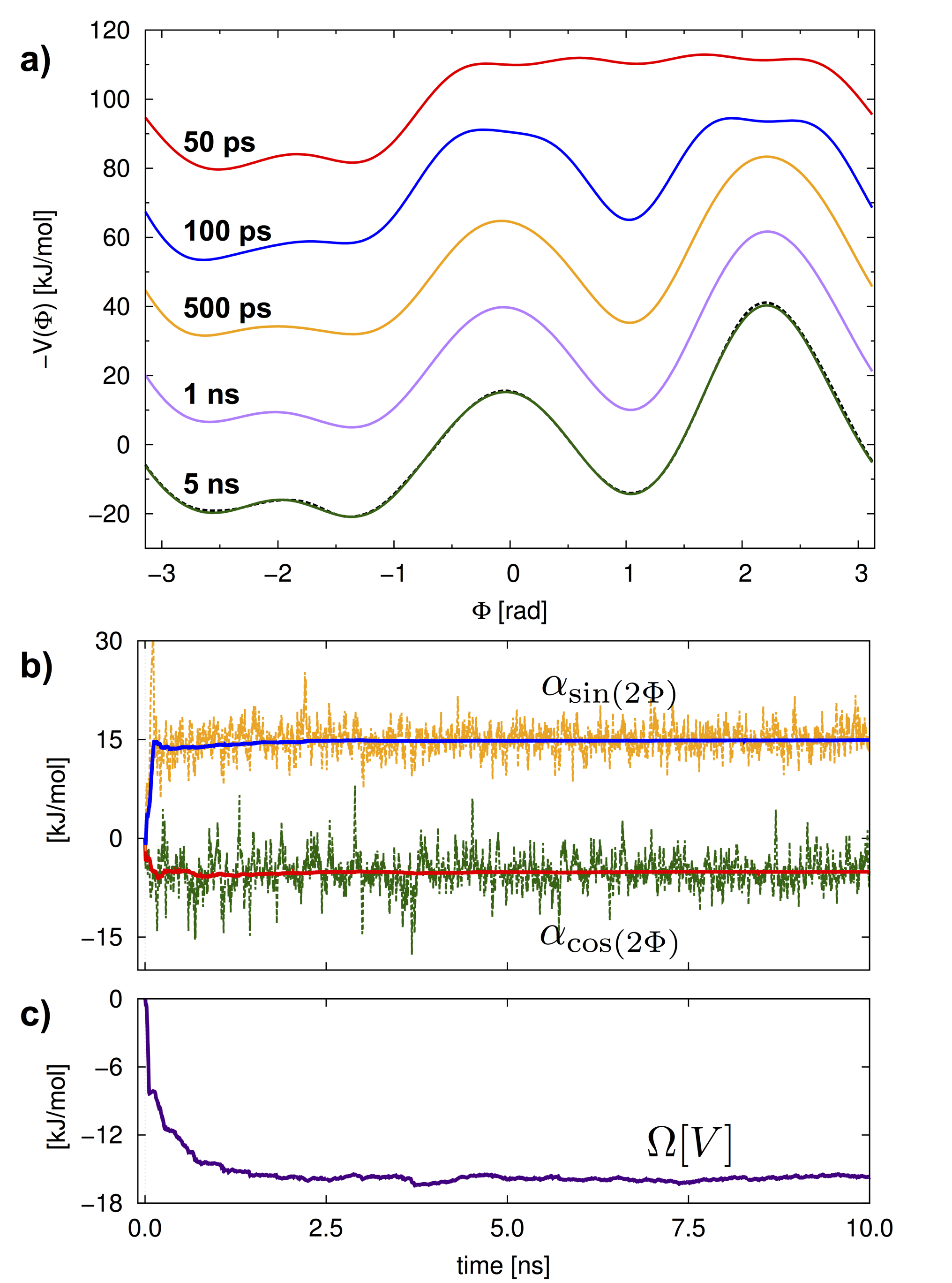
Figure 1: (Color online) Time evolution of the bias potential during minimization for alanine dipeptide in vacuum at 300 K. Only the backbone dihedral angle $\Phi$ acts as CV and 12 basis functions are included in the expansion of $V(\Phi)$. a) The $F(\Phi)$ as estimated by the negative of the bias potential (for clarity the potentials are shifted relative to one another by 25 kJ/mol). At 5 ns we also compare our variational result with a fully converged estimate of the FES from well-tempered metadynamics (black dashed line). The two curves are almost indistinguishable. b) Time evolution of the instantaneous and average expansion coefficients of $\cos(2\Phi)$ and $\sin(2\Phi)$. c) Time evolution $\Omega[V]$ estimated by a running average from the start of the simulation (see SM).

It has become customary to test any new free energy method on alanine dipeptide in vacuum and we shall adhere to this tradition. Conventionally the FES of alanine dipeptide is described in terms of the two backbone dihedral angles $\Phi$ and $\Psi$ (see SM) but in vacuum only the $\Phi$ angle is a slow degree-of-freedom while $\Psi$ can be considered as a fast degree-of-freedom. Therefore, by biasing only $\Phi$ one can still obtain a proper sampling of phase space. In Fig. 1 we show the evolution of the minimization process when using only the backbone dihedral angle $\Phi$ as CV. It is seen that in this case the bias potential $V(\Phi)$ evolves in a manner resembling that of standard metadynamics, filling progressively all the different minima and smoothly converging to the reference free energy profile $F(\Phi)$ obtained with metadynamics. In the same figure we also show two randomly chosen coefficients in the expansion of $V(\Phi)$ where we observe that while their instantaneous values oscillates greatly their averages converge smoothly. The same convergent behaviour is observed in the value of $\Omega[V]$ in Fig. 1c. We have also performed a conventional calculation using both backbone dihedral angles $\Phi$ and $\Psi$ as CVs with similar satisfactory results (see SM). Solvating the alanine dipeptide in explicit water and using the two traditional CVs also leads to gratifying results (see SM).

As noted earlier in many cases the FES are rather smooth functions so one can obtain a good representation of $V(\mathbf{s})$ with only a minimal basis set. In alanine dipeptide both in vacuum and in water we obtain already a rather good description of the FES with only 7 basis functions per CV. We make use of this ability of representing the FES with a minimal basis set in our next example.

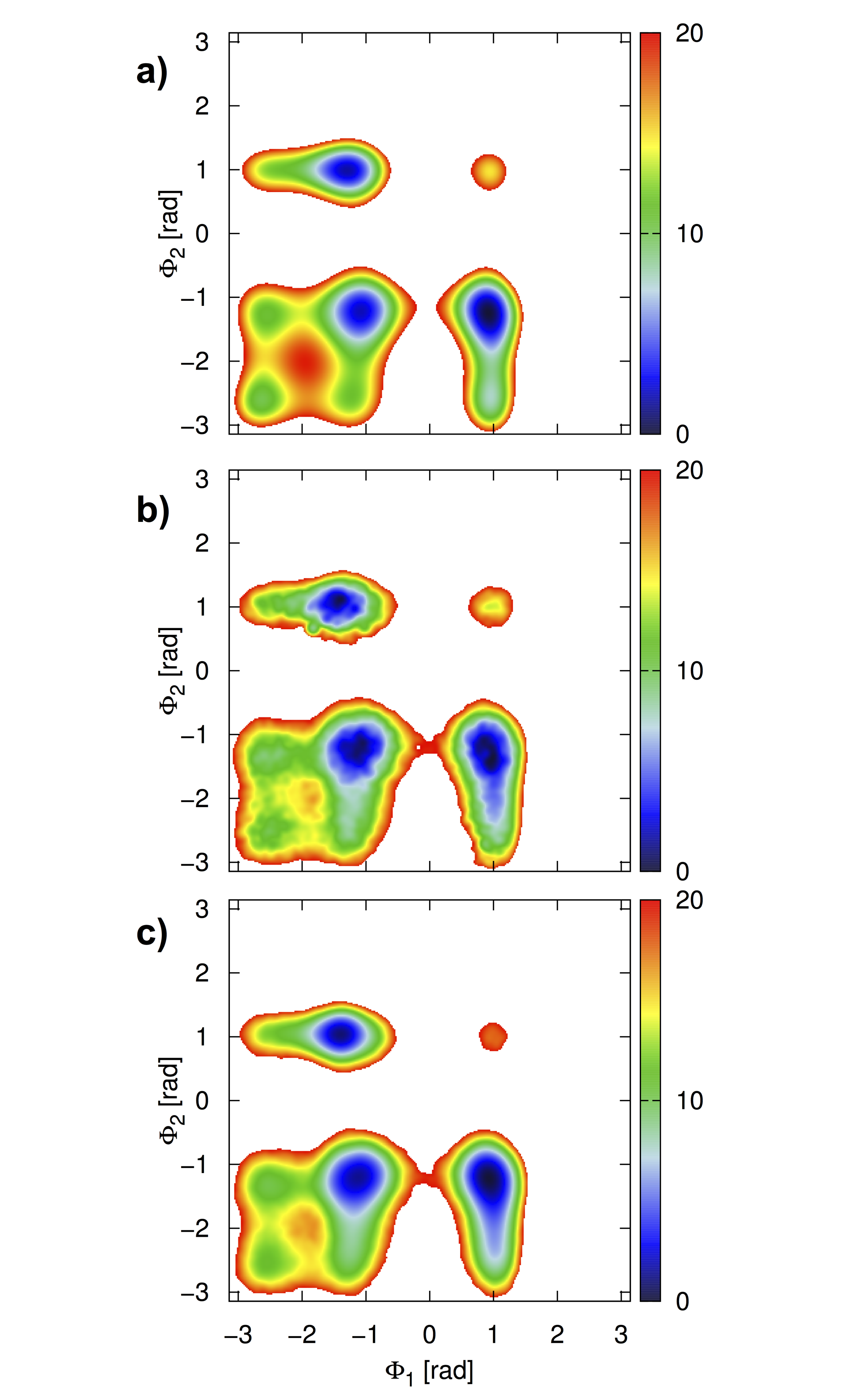
Figure 2: (Color online) The two-dimensional FES $F(\Phi_{1},\Phi_{2})$ obtained with the variational approach for Ala₃ in vacuum at 300K using the backbone dihedral angles $\Phi_{1}$, $\Phi_{2}$, and $\Phi_{3}$ as CVs and 342 basis functions in the expansion of $V(\Phi_{1},\Phi_{2},\Phi_{3})$. a) FES obtained from a projection of $F(\Phi_{1},\Phi_{2},\Phi_{3})$. b) FES obtained with on the fly reweighting. c) Reference results from a 500 ns parallel tempering simulation (8 replicas with an aggregated simulation time of 4 $\mu$s). The color scale of the FES is given in units of kJ/mol. All FES have their minimum value set to zero and are cut such that regions higher than 8 $k_{\textrm{B}}T$ ($\approx 20$ kJ/mol) are not shown. See SM for further details.

This is the more challenging case of a Ala₃ peptide in vacuum. While its conformations are described by its six backbone dihedral angles $\Phi_{1}$,$\Psi_{1}$,$\Phi_{2}$,$\Psi_{2}$,$\Phi_{3}$,$\Psi_{3}$ (see SM) only the three $\Phi$ angles suffice as CVs. As we increase the dimensionality of the CV space the number of variational parameters increases exponentially with $d$. To keep the number of variational parameters small we shall only use a minimal basis set. In the Ala₃ case this leads to use only 342 basis functions. With this choice during optimization all three CVs quickly become diffusive and the bias potential $V(\Phi_{1},\Phi_{2},\Phi_{3})$ converges after 50-100 ns of simulation time.

Despite employing a minimal basis we get a rather good representation of the FES as shown in Fig. 2 where we present a two-dimensional projection of $F(\Phi_{1},\Phi_{2},\Phi_{3})$ on $\Phi_{1}$ and $\Phi_{2}$ (projections for the other CVs can be seen in the SM). Any lack of full variational flexibility in the bias potential can furthermore be fully corrected by performing an on the fly reweighting during the optimization process. As observed in Fig. 2 the FES obtained in this manner are in excellent agreement with reference results from an extensive 500 ns parallel-tempering simulation. In the SM we show furthermore reweigthed FES for other CVs not biased during the simulation that also are in excellent agreement with the reference results.

While this approach offers a significant improvement over metadynamics and other similar methods its usefulness still depends on an appropriate choice of the CVs. Like in metadynamics, a poor choice of the CVs will manifest itself in a hysteretical behaviour during the optimization process (see SM). However our variational approach with its potential for handling many CVs can greatly alleviate the problem. A further help in this direction is the possibility of adding variational flexibility in the definition of the CVs.

To improve upon the method we can borrow all the ideas that have been applied to metadynamics like parallel tempering Bussi et al. (2006), multiple walkers Raiteri et al. (2006), or bias-exchange Piana and Laio (2007). Furthermore, metadynamics itself can be used to sample the averages needed in Eqs. 6 and A Variational Approach to Enhanced Sampling and Free Energy Calculations by employing a recent improved reweighting scheme Tiwary and Parrinello (2014). The sampling power of the variational approach can thus be further enhanced by biasing the metadynamics with CVs different from $\mathbf{s}$.

The main result of this paper is the introduction of the functional $\Omega[V]$ and the practical demonstration of its usefulness. We believe that there is ample room for improvement. The optimization procedure presented here is not necessarily optimal and different systems and CVs might require different optimization strategies and different basis set. We plan to explore a number of alternative procedures. For instance one could think of setting up an iterative procedure in which an approximate calculation is made for $F_{0}(\mathbf{s})$ using Eq. 3 at the early stages of the calculation. One can then insert into Eq. 2 a new $p_{0}(\mathbf{s})=\frac{e^{-\beta F_{0}(\mathbf{s})}}{\int d\mathbf{s}\,e^{-\beta F_{0}(\mathbf{s})}}$. The resulting functional is then optimized and the procedure iterated until at convergence after $k$ steps $p_{k}(\mathbf{s})=\frac{e^{-\beta F_{k}(\mathbf{s})}}{\int d\mathbf{s}\,e^{-\beta F_{k}(\mathbf{s})}}$ and $V_{k}(\mathbf{s})\approx 0$ to the desired accuracy.

These brief discussion on the potential for improvements and modifications of the scheme is by far not exhaustive but is meant to indicate some of the future lines of investigation and indicate the in this very first application we are only using a small fraction of the potentialities of this method and that much more exciting developments are to be expected. We would also like to point out the potential of our method in the development of a more rigorous coarse graining procedure.

Finally we note that the systems considered here are by necessity simple, as conventionally done when introducing a completely new method. The strengths and limitations of our approach will become clearer as it is further developed.

The method has been implemented in a development version of the PLUMED 2 Tribello et al. (2014) plug-in and will be made publicly available in the coming future.