Conservative Signal Processing Architectures
For Asynchronous, Distributed Optimization
Part II: Example Systems

Abstract

This paper provides examples of various synchronous and asynchronous signal processing systems for performing optimization, utilizing the framework and elements developed in a preceding paper. The general strategy in that paper was to perform a linear transformation of stationarity conditions applicable to a class of convex and nonconvex optimization problems, resulting in algorithms that operate on a linear superposition of the associated primal and dual decision variables. The examples in this paper address various specific optimization problems including the LASSO problem, minimax-optimal filter design, the decentralized training of a support vector machine classifier, and sparse filter design for acoustic equalization. Where appropriate, multiple algorithms for solving the same optimization problem are presented, illustrating the use of the underlying framework in designing a variety of distinct classes of algorithms. The examples are accompanied by numerical simulation and a discussion of convergence.

I Introduction

This paper presents various classes of asynchronous, distributed optimization systems, demonstrating the use of the framework discussed in Part I [1]. The design and use of each class of systems is based upon the following strategy:

1. Write a reduced-form optimization problem, defined in [1].

2. Connect appropriate constitutive relations to interconnection elements, e.g. from Figs. 2-3 in [1], implementing the associated transformed stationarity conditions. Delay-free loops will generally result.

3. Break delay-free loops:

   1. For any constitutive relation that is a source element, perform algebraic simplification thereby incorporating the solution of the algebraic loop into the interconnection.

   2. Insert synchronous or asynchronous delays between the remaining constitutive relations and the interconnection.

4. Run the distributed system until it reaches a fixed point. The discussion in Section III, in conjunction with the system properties in Fig. 3 in [1], provide guidance in determining when convergence is ensured.

5. Read out the primal and dual decision variables $a_{i}$ and $b_{i}$ by multiplying the variables $c_{i}$ and $d_{i}$ by the inverses of the ($2\times 2$) matrices used in transforming the stationarity conditions.

II Example Systems

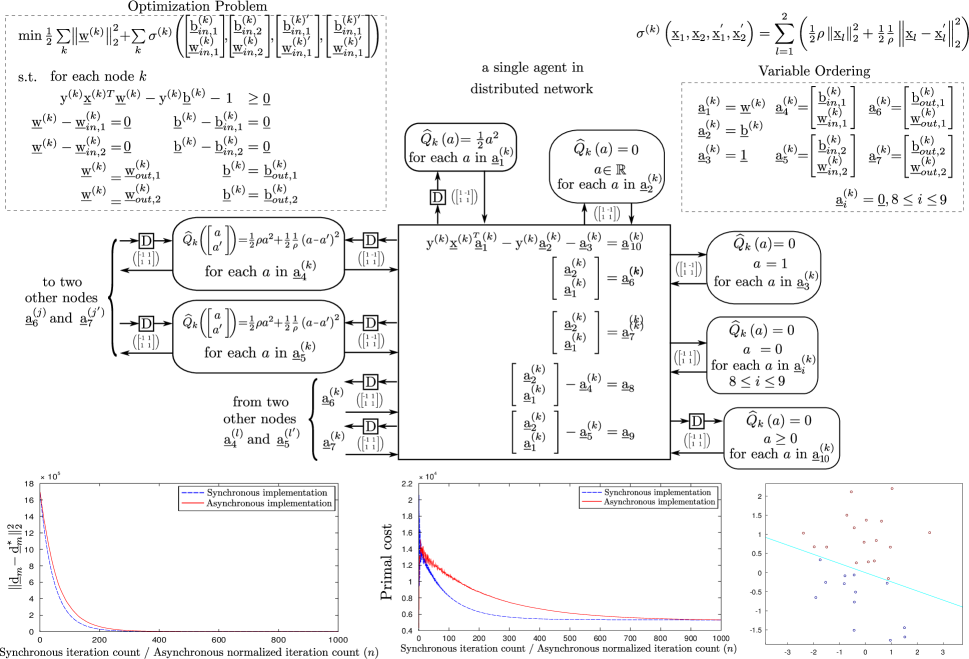
Figure 6: Signal processing architecture for a single agent in a connected graph implementing a decentralized algorithm for training a support vector machine classifier. The numerical simulation depicts a system involving $30$ such agents, each having knowledge of a single training vector. The parameter $\rho$ specifies the relative enforcement of equality for the system variables that are coupled between each agent in the graph. For the depicted solution $\rho$ is selected to be small, and the graph is known to be connected, with each node as depicted above having exactly four incident connections.

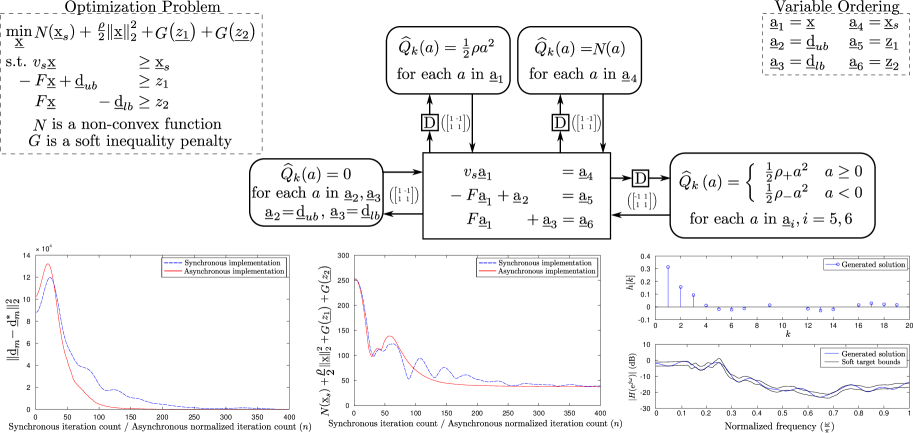
Figure 7: Signal processing architecture and numerical simulation corresponding to a nonconvex sparse filter design problem. The parameters $\rho$ and $v_{s}$ are respectively selected to specify the enforcement of the size of $\underline{\mbox{x}}$ and the width of the abrupt decrease in cost about $0$ for the nonconvex element. $\rho_{+}$ and $\rho_{-}$ affect the enforcement of the soft inequality constraints. For the depicted solution $\rho$ and $\rho_{+}$ are selected to be small and $\rho_{-}$ and $v_{s}$ are selected to be large.

Figs. 3-7 depict various asynchronous, distributed optimization algorithms implemented using the presented framework, specifically making use of the elements in Figs. 2-3 of Part I [1]. Figs. 3 and 3 in this paper illustrate two alternative implementations of systems for solving the LASSO problem. Figs. 4 and 5 depict two alternative implementations of systems for performing minimax-optimal FIR filter design. Fig. 6 depicts a support vector machine classifier trained using a decentralized algorithm generated using the presented framework. Fig. 7 illustrates an example of a nonconvex optimization algorithm aimed at the problem discussed in [2], in particular that of designing a sparse FIR filter for acoustic equalization. In Figs. 3-7, the asynchronous delay elements were numerically simulated using discrete-time sample-and-hold systems triggered by independent Bernoulli processes, with the probability of sampling being $0.1$.

III Discussion of convergence

Fig. 1(a) summarizes the overall interconnection of elements composing the presented class of systems discussed in Part I [1], with those maps $m_{k}(\cdot)$ corresponding to source relationships being written separately. Figs. 1(b)-(d) illustrate a set of manipulations useful in analyzing convergence, with Fig. 1(b) specifically depicting a solution to the transformed stationarity conditions. The approach is to begin with the system in Fig. 1(a) and perform the additions and subtractions of $c^{\star}_{i}$ and $d^{\star}_{i}$ indicated in Fig. 1(c), obtaining Fig. 1(d) by identifying that Fig. 1(c) is a superposition of Figs. 1(b) and (d).

Figure 1: (a) General description of the interconnection of elements used in the presented systems. (b)-(d) Manipulations performed in analyzing convergence.

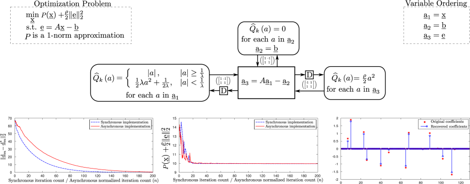
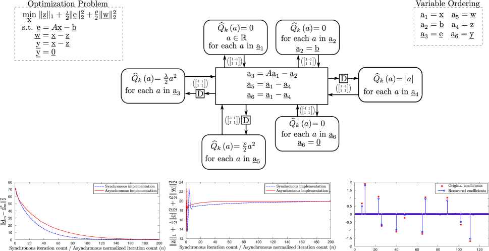
Figure 2: Signal processing architecture and numerical simulation corresponding to an algorithm for solving the LASSO problem. An approximation to the $1$-norm is used that is quadratic in the close vicinity of $0$. The parameters $\lambda$ and $\rho$ are selected to specify the interval outside of which the $1$-norm approximation is exact and to trade off between the sparsity of the solution and the enforcement of the linear equality constraints, respectively. For the depicted solution $\lambda$ and $\rho$ are selected to be large. Note in particular the monotonic convergence of $||\underline{d}_{m}-\underline{d}_{m}^{\star}||^{2}_{2}$ to zero. “Asynchronous normalized iteration count” indicates the number of iterations times the probability of sampling, discussed in Section II.

Figure 3: Signal processing architecture and numerical simulation for an augmented-cost LASSO problem, with the cost being augmented similarly to that of various ADMM formulations.[3] The augmentation parameter is denoted $\rho$. The parameter $\lambda$ is selected to trade off between the sparsity of the solution and the enforcement of the linear equality constraints. For the depicted solution $\lambda$ and $\rho$ are selected to be large.

There are various ways that the system in Fig. 1(d) can be used in determining sufficient conditions for convergence, a subset of which we outline here. Generally, arguments for convergence utilizing Fig. 1(d) involve identifying conditions for which $||\underline{d}_{D}||$ in this figure is strictly less than $||\underline{d}^{\prime}_{m}||$, except at $0$. Using the definition of a source element in [1] and the fact that $G$ is a neutral map, i.e. an orthonormal matrix, we conclude from Fig. 1(d) that

$$||\underline{d}_{D}||\leq||\underline{c}^{\prime}_{m}||.$$ (1)

If, for example, the solution to the transformed stationarity conditions $c^{\star}_{i}$ and $d^{\star}_{i}$ is known to be unique, and additionally if the collection of constitutive relations denoted $m(\cdot)$ is known to be dissipative about $\underline{d}_{m}^{\star}$, then from Fig. 1(d) we conclude that $||\underline{c}^{\prime}_{m}||<||\underline{d}^{\prime}_{m}||$ except at $0$, resulting in

$$||\underline{d}_{D}||<||\underline{d}^{\prime}_{m}||$$ (2)

except at $0$. Eq. 2 implies, for example, that coupling the constitutive relations denoted $m(\cdot)$ to the linear interconnection elements via deterministic vector delays, the discrete-time signal denoted $\underline{d}^{\prime}_{m}[n]$ will converge to $0$ and so the signal $\underline{d}_{m}[n]$ will converge to $\underline{d}^{\star}_{m}$.

The uniqueness of the stationarity conditions and the property of the constitutive relations being dissipative used in the preceding argument are not, however, strictly required. A more general line of reasoning involves justifying Eq. 2 in the vicinity of any such solution $c^{\star}_{i}$ and $d^{\star}_{i}$, for example by claiming that even if specific constitutive relations $m_{k}(\cdot)$ are norm-increasing, the overall interconnected system results in a map from $\underline{d}^{\prime}_{m}$ to $\underline{d}_{D}$ that is norm-reducing in the vicinity of that solution.

Arguments for convergence involving essentially Eq. 2 can also be applied in a straightforward way to systems utilizing asynchronous delays, modeled as discrete-time sample-and-hold systems triggered by independent Bernoulli processes. In particular by taking the expected value of $||\underline{d}^{\prime}_{(m)}[n]||$, applying the law of total expectation, substituting in Eq. 2, and performing algebraic manipulations, it can be argued that $E[||\underline{d}^{\prime}_{(m)}[n]||]$ converges to $0$. A more formal treatment of convergence is the subject of future work.

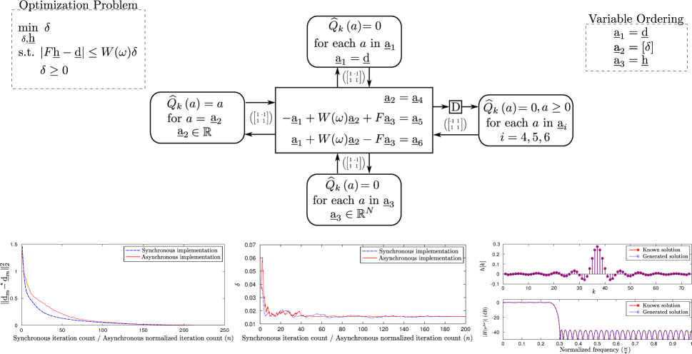
Figure 4: Signal processing architecture and numerical simulation corresponding to a minimax-optimal FIR filter design problem, specifically that of lowpass filter design. The obtained result is compared with a known solution from the Parks-McClellan algorithm.

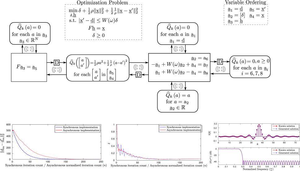
Figure 5: Alternative algorithm for minimax-optimal filter design, obtained by modification of the problem statement in Fig. 4 and intended to demonstrate that the presented framework can be used in designing a variety of distinct classes of algorithms. The parameter $\rho$ is selected to specify the relative enforcement of equality between the system variables loosely shared between the two linear interconnection elements. For the depicted solution $\rho$ is selected to be small, resulting in a very close approximation to the lowpass filter design problem in Fig. 4.

References

- [1] T. A. Baran and T. A. Lahlou, “Conservative signal processing architectures for asynchronous, distributed optimization part I: General framework,” in Proc. of IEEE Global Conference on Signal and Information Processing (GlobalSIP), 2014.
- [2] T. Baran, D. Wei, and A. V. Oppenheim, “Linear programming algorithms for sparse filter design,” Signal Processing, IEEE Transactions on, vol. 58, no. 3, pp. 1605–1617, 2010.
- [3] S. Boyd, N. Parikh, E. Chu, B. Peleato, and J. Eckstein, “Distributed optimization and statistical learning via the alternating direction method of multipliers,” Found. Trends Mach. Learn., 2011.
- [4] T. A. Baran, Conservation in Signal Processing Systems, Ph.D. thesis, Massachusetts Institute of Technology, 2012.
- [5] A. Fettweis, “Wave digital filters: Theory and practice,” Proceedings of the IEEE, vol. 74, no. 2, pp. 270–327, Feb 1986.
- [6] L. O. Chua and G. N. Lin, “Nonlinear programming without computation,” Circuits and Systems, IEEE Transactions on, vol. 31, no. 2, pp. 182–188, Feb 1984.
- [7] J. B. Dennis, Mathematical Programming and Electrical Networks, Ph.D. thesis, Massachusetts Institute of Technology, 1958.
- [8] M. P. Kennedy and L. O. Chua, “Neural networks for nonlinear programming,” Circuits and Systems, IEEE Transactions on, vol. 35, no. 5, pp. 554–562, May 1988.
- [9] W. Millar, “Some general theorems for non-linear systems possessing resistance,” Philosophical Magazine Series 7, vol. 42, no. 333, pp. 1150–1160, 1951.
- [10] J. Wyatt, “Little-known properties of resistive grids that are useful in analog vision chip designs,” Vision Chips: Implementing Vision Algorithms with Analog VLSI Circuits, pp. 72–89, 1995.
- [11] P. Penfield, R. Spence, and S. Duinker, Tellegen’s Theorem and Electrical Networks, The MIT Press, 1970.
- [12] B. D. H. Tellegen, “A general network theorem, with applications,” Tech. Rep., Philips Research Reports, Philips Research Reports.
- [13] J. C. Willems, “Dissipative dynamical systems part I: General theory,” Archive for Rational Mechanics and Analysis, vol. 45, pp. 321–351, jan 1972.
- [14] J. C. Willems, “The behavioral approach to open and interconnected systems,” Control Systems, IEEE, vol. 27, no. 6, pp. 46–99, Dec 2007.
- [15] T. A. Baran and B. K. P. Horn, “A robust signal-flow architecture for cooperative vehicle density control,” in Acoustics, Speech and Signal Processing (ICASSP), 2013 IEEE International Conference on, May 2013, pp. 2790–2794.
- [16] S. K. Rao and T. Kailath, “Orthogonal digital filters for vlsi implementation,” Circuits and Systems, IEEE Transactions on, vol. 31, no. 11, pp. 933–945, Nov 1984.
- [17] E. Deprettere and P. Dewilde, “Orthogonal cascade realization of real multiport digital filters,” International Journal of Circuit Theory and Applications, vol. 8, no. 3, pp. 245–272, 1980.
- [18] N. Parikh and S. Boyd, “Block splitting for distributed optimization,” Mathematical Programming Computation, 2014.
- [19] P. A. Forero, A. Cano, and G. B. Giannakis, “Consensus-based distributed support vector machines,” J. Mach. Learn. Res., 2010.
- [20] E. Wei and A. Ozdaglar, “Distributed alternating direction method of multipliers,” in Decision and Control (CDC), 2012 IEEE 51st Annual Conference on, Dec 2012, pp. 5445–5450.