Polarized solutions and Fermi surfaces in holographic Bose-Fermi systems

Abstract:

We use holography to study the ground state of a system with interacting bosonic and fermionic degrees of freedom at finite density. The gravitational model consists of Einstein-Maxwell gravity coupled to a perfect fluid of charged fermions and to a charged scalar field which interact through a current-current interaction. When the scalar field is non-trivial, in addition to compact electron stars, the screening of the fermion electric charge by the scalar condensate allows the formation of solutions where the fermion fluid is made of antiparticles, as well as solutions with coexisting, separated regions of particle-like and antiparticle-like fermion fluids. We show that, when the latter solutions exist, they are thermodynamically favored. By computing the two-point Green function of the boundary fermionic operator we show that, in addition to the charged scalar condensate, the dual field theory state exhibits electron-like and/or hole-like Fermi surfaces. Compared to fluid-only solutions, the presence of the scalar condensate destroys the Fermi surfaces with lowest Fermi momenta. We interpret this as a signal of the onset of superconductivity.

1 Introduction

The holographic correspondence between field theories in $d$ dimensions and gravitational theories in $d+1$ dimension has been extensively used to study properties of strongly coupled systems, obtaining information that is not easily accessible by ordinary methods. In particular, fermionic systems at finite density pose a particularly difficult problem, as there are no theoretical models that can be studied reliably in a controlled approximation and lattice simulations are marred by the “sign problem”. In this context, the holographic method has proved useful by offering a number of insights into possible exotic phases of matter that are not described by Landau’s theory of Fermi liquids or other weakly-coupled descriptions [1, 2, 3, 4].

It was suggested in [5] that the presence of a charged horizon in the simplest gravity solutions dual to finite-density states admits an interpretation in terms of fractionalization of the fundamental charged degrees of freedom. When the charge is sourced by matter fields in the bulk, it corresponds to fermionic operators in the boundary. But when the charge emanates from the horizon, it cannot be associated to any gauge-invariant observable. This leads to a violation of the Luttinger’s theorem: the charge contained in the Fermi surface (or surfaces) does not account for the total charge of the system. The phase transition corresponding to the onset of fractionalization was studied in [6, 7, 8]. When there are charged scalars in the theory, they can also become excited and condense, carrying part of the charge. In this case however the $U(1)$ symmetry is broken, and the interpretation is different: the system undergoes a transition to a superconducting state [7]. If both components are allowed to be present, there can be a competition between the bosons and the fermions . We have considered this situation in a previous paper [16] where we studied gravitational solutions in which the charged matter in the bulk can be both fermionic and bosonic, in the regime where the fermions can be treated as a perfect fluid. We have found phase transitions between the electron star, the holographic superconductor, and a new class of solutions in which the electron star is dressed by a scalar condensate. We called them compact stars since they extend only across a finite range in the radial direction of the bulk geometry: the fermionic fluid is confined in a radial shell, and the infrared geometry is the same as for the zero-temperature holographic superconductor of [17]. A similar system was studied in [18], but with a different potential that also allows for an unbounded fluid with Lifshitz asymptotics in the IR.

In the present paper, we continue the study of the system analyzed in [16], adding a new ingredient, namely a direct coupling between the scalar and the fermions. The reason for introducing this coupling is the following: in the holographic superconductor, the boundary bosonic operator that develops a vacuum expectation value is interpreted as a strongly coupled analogue of the Cooper pair that condenses in the superconducting state in the usual BCS theory. In our model fermions are also present at the same time, so if the boson has to be interpreted as a bound state of fermions, it seems unnatural that they should interact only from the exchange of gauge fields. A natural interaction term would be a Yukawa coupling, as it was considered in [19]. This requires dealing with microscopic fermions and going away from the fluid approximation; moreover the coupling can only be there in the case where the boson has twice the charge of the fermions.

In [20], an interacting description in the fluid approximation was given that treats the scalar as a BCS-like fermion bilinear. In the fluid approximation, the presence of the condensate modifies the fermionic fluid equation of state. At the macroscopic level, this system too may arise from a Yukawa interaction of a scalar whose charge is twice that of the elementary fermions.

In a strongly coupled system we cannot discard the possibility that the fermions that condense are not the fundamental electrons but some other excitation, perhaps fractionalized, therefore we want to leave the ratio of the charges arbitrary.

If we want to work directly with the fluid approximation, and at the same time leave the scalar and fermion charges generic, the simplest interaction we can write is a current-current coupling. We found that in the presence of this interaction, a surprising phenomenon takes place: in the bulk we can have a polarized charged system, which is constituted of radially separated shells of positively and negatively charged components of the fluid, immersed in a non-zero scalar condensate. We call these solutions electron-positron stars, and they are illustrated schematically in Figure 1.

Figure 1: Structure of compact electron-positron star solutions. The bulk fermion fluid is confined within two spherical shells: the outer shell (green) is made out of particles (electrons) and the inner one (red) is made of holes (positrons). The whole configuration is immersed in the non-zero bulk scalar condensate, which overscreens the hole-like fluid making it effectively repel the particle shell. This combination of electromagnetic repulsion and gravitational attraction renders the system stable.

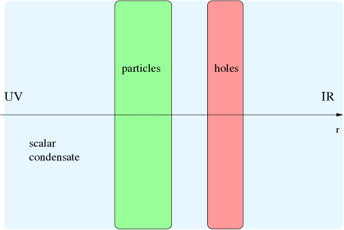
The reason these solutions may arise is that, due to the current-current interaction term, the local chemical potential can have opposite signs in different regions of the bulk geometry. This leads to both fermionic particles and antiparticles being populated in separate regions. The solution is stable because the scalar condensate effectively screens the negative charge of the positrons so that these do not feel the electric attraction of the electrons but rather they are repelled. The system is kept together by the gravitational attraction, which balances the electromagnetic repulsion.

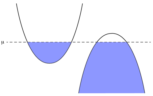
The simplest boundary interpretation of these solutions appears to be in terms of different flavors of fermions, each of them having a certain band structure but with the zero energy level having a different offset for different flavors, so that a given chemical potential intersects the conductance band for some fermions and the valence band for others (see Figure 2 for a schematic representation of this phenomenon). We do not know of any realistic system that displays such features, it would be interesting to find some real-world realization of this situation.

Figure 2: Schematic band structure of (dual of) the compact polarized stars solutions.

To shed more light on the physics of the system, we study the spectrum of low-energy fermionic excitations. We consider a probe fermion in the geometry, that is also interacting with the Maxwell field and with the scalar current, since it is supposed to be one of the fermions making up the fluid. We solve the Dirac equation in the WKB approximation and find the normal and quasi-normal modes, that correspond to poles of the boundary fermionic Green’s function. The analysis of the poles at zero frequency and finite momentum reveals the presence of a finite number of Fermi surfaces.

One can compare this situation with that of the unbounded electron star in the absence of the scalar field [21]. In the latter case, there are infinitely many Fermi surfaces, with Fermi momenta accumulating exponentially close to zero. As discussed in [22], the dual field theory interpretation is that of a Fermi system in a limit where the number of constituent fermions is infinite. In compact stars (both in the electron and the electron-positron version) there are only finitely many Fermi surfaces, meaning that all except for a finite number of Fermi surfaces become gapped due to the scalar condensate. For small frequency, in the electron star the modes have a small dissipation due to the possibility of tunneling into the IR Lifshitz part of the geometry. This was interpreted as the effect of the interaction of the fermions with bosonic critical modes. In compact star solutions, on the other hand, we find that for a certain range of energies above zero, the excitations are stable, so there is no residual interaction at low energies. The comparison with the electron star also reveals that the most “shallow” modes, corresponding to Fermi surfaces with smallest momenta, are the ones that disappear from the spectrum; we interpret this as a signal that the system has become gapped due to the superconductivity; however the gap concerns only part of the system, as other Fermi surfaces remain gapless. Naively one would expect that the smallest Fermi surfaces should be more robust, since they have a lower temperature for the superconducting transition, as predicted by BCS [19]. A possible explanation would be if the mechanism for superconductivity is not described by BCS. In fact, our findings are consistent with the UV/IR duality displayed by holographic Fermionic fluids discussed in [22], where it was argued that the states corresponding to the smallest Fermi momenta are the last to be filled.

The plan of the paper is as follows: in Section 2 we review the results of our previous work, in particular the compact star solutions. In Section 3 we study the system in presence of the current-current coupling and describe the new solutions, find the free energy and determine the phase diagram. In Section 4 we analyze the probe fermions and determine the low-energy spectrum. We conclude in Section 5 summarizing the results and indicating the open questions and future directions of investigation.

2 Bosonic and fermionic matter in asymptotically AdS spacetimes

We will consider four-dimensional gravitational solutions which are asymptotically $AdS_{4}$ and have zero temperature and finite charge density. These solutions arise from models which have an action of the form

$$S=\int\mathrm{d}^{4}x\sqrt{-g}\left[\frac{1}{2\kappa^{2}}\left(R+\frac{6}{L^{2}}\right)-\frac{1}{4e^{2}}F_{ab}F^{ab}\right]+S_{\textnormal{matter}}+S_{\textnormal{bdry}}$$ (2.1)

where $F=\mathrm{d}A$ is the field strength of the gauge field $A$, $\kappa$ is Newton’s constant, $L$ is the asymptotic $AdS_{4}$ length and $e$ is the $U(1)$ coupling. The term $S_{\textnormal{bdry}}$ represents the Gibbons-Hawking term and the counterterms necessary for the holographic renormalization and $S_{\textnormal{matter}}$ is the action for the matter fields.

As in [16, 18], we will consider the simultaneous presence of two types of bulk matter:

1. A charged scalar field $\psi$ with action:

   $$S_{\textnormal{scalar}}=-\frac{1}{2}\int\mathrm{d}^{4}x\sqrt{-g}\left(\left|\nabla\psi-iqA\psi\right|^{2}+m_{s}^{2}|\psi|^{2}\right)\,,$$ (2.2)

   where $q$ is the scalar field $U(1)$ charge and $m_{s}^{2}$ is negative and satisfies the Breitenlohner-Freedman (BF) bound, $-9/4<L^{2}m_{s}^{2}<0$.

2. A fermionic component described effectively by a fluid stress tensor and electromagnetic current:

   $$T_{ab}^{\textnormal{fluid}}=(\rho+p)u_{a}u_{b}+pg_{ab}\,,\qquad J^{a}_{\textnormal{fluid}}=\sigma u^{a}\,.$$ (2.3)

   The form of the fluid energy density $\rho$, pressure $p$ and charge density $\sigma$ will be given shortly.

We will restrict to static, homogeneous and isotropic solutions, which by performing diffeomorphisms and gauge transformations can always be written as,

$$\mathrm{d}s^{2} =L^{2}\left[-f(r)\mathrm{d}t^{2}+g(r)\mathrm{d}r^{2}+\frac{1}{r^{2}}\left(\mathrm{d}x^{2}+\mathrm{d}y^{2}\right)\right]\,,$$ (2.4)

$$A =\frac{eL}{\kappa}h(r)\mathrm{d}t\ ,\qquad\psi=\psi(r)\,,\qquad u^{a}=(u^{t}(r),0,0,0)\,,$$

in which $r=0$ is the $AdS$ boundary. As discussed in detail in Appendix A, we rescale all quantities by suitable powers of $e$, $L$ and $\kappa$ and denote the rescaled quantities with hats. In the UV region we have:

$$r\to 0:\qquad f(r)\sim\frac{1}{r^{2}}\,,\qquad h(r)\sim\hat{\mu}-\hat{Q}r\,,$$ (2.5)

where $\hat{\mu}$ is the chemical potential of the boundary quantum field theory and $\hat{Q}$ the total charge of the system. We will assume that the UV asymptotics of the scalar field corresponds to zero source term for the dual operator, i.e.:

$$\psi\sim\psi_{+}\,r^{\Delta}\,,\qquad\Delta=\frac{3}{2}+\frac{3}{2}\sqrt{1+\frac{4\hat{m}_{s}^{2}}{9}}\,,$$ (2.6)

where $\Delta$ is the conformal dimension of the field theory scalar operator $\mathcal{O}$.

The energy density $\rho$, pressure $p$, charge density $\sigma$ and fluid velocity $u^{a}$ are assumed to locally satisfy the chemical equilibrium equation of state of a free Fermi gas, as in [23], with a density of states given by:

$$g(\epsilon)=\left\{\begin{array}[]{lr}\beta\,\epsilon\,\sqrt{\epsilon^{2}-m_{f}^{2}}&\qquad\epsilon>m_{f}\,,\\ 0&\qquad 0<\epsilon<m_{f}\,,\end{array}\right.$$ (2.9)

where $m_{f}$ is the constituent fermion mass and $\beta$ is a phenomenological parameter related to the spin of the fermions.

It is convenient to describe the fluid using rescaled energy density, pressure and charge density (defined in Appendix A.1 and denoted by a hat), which under the local chemical equilibrium condition are given by:

$$\hat{\rho}(r) =\hat{\beta}\int_{\hat{m}_{f}}^{|\hat{\mu}_{l}(r)|}\mathrm{d}\epsilon\ \Theta\left(\epsilon-\hat{m}_{f}\right)\epsilon^{2}\,\sqrt{\epsilon^{2}-\hat{m}_{f}^{2}}\,,$$ (2.10)

$$\qquad\hat{\sigma}(r) =\textnormal{sign}(\hat{\mu}_{l})\,\hat{\beta}\int_{\hat{m}_{f}}^{|\hat{\mu}_{l}(r)|}\mathrm{d}\epsilon\ \Theta\left(\epsilon-\hat{m}_{f}\right)\epsilon\,\sqrt{\epsilon^{2}-\hat{m}_{f}^{2}}\,,$$ (2.11)

$$-\hat{p}(r) =\hat{\rho}(r)-\hat{\mu}_{l}(r)\hat{\sigma}(r)\,,$$ (2.12)

where $\hat{\mu}_{l}(r)$ is the local chemical potential in the bulk, defined in Appendix A, and

$$\hat{m}_{f}=\frac{\kappa}{e}\frac{m_{f}}{|q_{f}|}\,,\qquad\hat{\beta}=\frac{e^{4}L^{2}}{\kappa^{2}}\beta q_{f}^{4}\,,$$ (2.13)

where $q_{f}$ is the elementary charge of the constituent fermions.

With respect to the original construction in [23], we allow for both signs of $q_{f}$, i.e. we allow for the possibility of the fluid to be made up of particles (electrons, $q_{f}>0$) and antiparticles (holes, or positrons, $q_{f}<0$). This leads to a slight generalization of equations (2.10) with respect to the original formulae of [23]. The details of how the signs and absolute values arise in (2.10) can be found in Appendix A.1. It is important to note that the sign of $\hat{\mu}_{l}(r)$ is the same as the sign of $q_{f}$, thus a negative chemical potential in the bulk will lead to the formation of a fluid made out of negatively charged constituents.

For $|\hat{\mu}_{l}|<m_{f}$, $\hat{\rho}=\hat{\sigma}=\hat{p}=0$ due to the Heaviside step functions, and there is no fluid.

The explicit expression of the local chemical potential depends on the way the fermions couple to the Maxwell and scalar field in the bulk. If there is no direct interaction between the scalar and fermionic components, it is given by

$$\hat{\mu}_{l}(r)=\frac{h(r)}{\sqrt{f(r)}}\,,$$ (2.14)

and it has the same sign of the electric potential $h(r)$ and of the boundary chemical potential $\hat{\mu}$ (Eq. (2.5)). For this reason, without direct interactions between the fermionic fluid and the scalar field, only positively charged solutions are possible for positive boundary chemical potential. This is the case covered in [23] and [16], and the possible bulk solutions are reviewed in the next subsection.

As we will see in Section 3, a direct current-current interaction between the fermion fluid and the scalar field will allow $\hat{\mu}_{l}(r)$ to have both signs, or even to change sign in the bulk, and solutions with both signs of the constituent fermion charge will be possible.

Finally, the local chemical equilibrium and Thomas-Fermi approximation, necessary for this description to be valid, require that

$$e^{2}\sim\frac{\kappa}{L}\ll 1\,.$$ (2.15)

2.1 Taxonomy of non-interacting solutions

The situation where bosonic and fermionic components do not have a direct interaction was analyzed in [16]. In this case, the expression of the local chemical potential is (2.14), and the possible homogeneous, charged, zero-temperature solutions of this system are listed below (the reader is referred to [16] for more details and to Appendix A for conventions and definitions of the rescaled variables).

Extremal RN-AdS Black hole (ERN).

In this case all the matter fields are trivial, the solution to the action (2.1) with metric and gauge field of the form (2.4) is the extremal Reissner-Nordström black hole. The infrared is an extremal horizon with geometry ${AdS_{2}\times\mathbb{R}^{2}}$.

Holographic Superconductor (HSC).

These are solution with non-vanishing scalar field (with vev-like UV asymptotics) but zero fluid density in the bulk [24, 25]. At zero temperature, the asymptotic solution in the IR ($r\to\infty$) is [17]

$$f(r) \sim\frac{1}{r^{2}}\,, g(r)\sim-\frac{3}{2\hat{m}_{s}^{2}}\frac{1}{r^{2}\log r}\,,$$ (2.16)

$$h(r) \sim h_{0}r^{\delta}\left(\log r\right)^{1/2}\,, \psi(r)\sim 2\left(\log r\right)^{1/2}\,,{}{}{}$$

where “hatted” quantities are defined in Appendix A, and $\delta<-1$. These solutions require the condition

$$\hat{q}^{2}>-\frac{\hat{m}_{s}^{2}}{3}$$ (2.17)

which will be always assumed in this paper.

Electron star (ES).

These solutions, first constructed in  [23], have a trivial scalar field, $\psi(r)=0$ but a non-vanishing fluid density in the bulk region where the local chemical potential $\hat{\mu}_{l}(r)$ exceeds the fermion mass $\hat{m}_{f}$. This happens in an unbounded region ${r_{s}<r<+\infty}$, $r_{s}$ representing the star boundary where $\hat{\rho}(r_{s})=\hat{\sigma}(r_{s})=0$ . Outside this region (i.e. for $0<r<r_{s}$) the solution coincides with the RN-AdS black hole described above. The region occupied by the fluid is unbounded, and in the far IR ($r\to\infty$), the fluid energy and charge density are constant and the geometry is asymptotically Lifshitz:

$$f(r)\sim\frac{1}{r^{2z}}\,,\qquad g(r)\sim\frac{g_{\infty}}{r^{2}}\,,\qquad h(r)\sim\frac{h_{\infty}}{r^{z}}\,,$$ (2.18)

where $g_{\infty}$ and $h_{\infty}$ are constants depending on $\hat{m}_{f}$ and $\hat{\beta}$, and the dynamical exponent $z$ is determined by

$$h_{\infty}=\sqrt{\frac{z-1}{z}}\,.$$ (2.19)

Compact electron stars (eCS).

Solutions with both a non-trivial scalar profile and a non-zero fluid density were found in [16]. The fluid density is confined in a shell $r_{1}<r<r_{2}$, whose boundaries are determined by the equation

$$\hat{\mu}_{l}(r_{1})=\hat{\mu}_{l}(r_{2})=\hat{m}_{f}\,.$$ (2.20)

The non-trivial scalar field profile is similar to the one of the holographic superconductor, and causes the local chemical potential to be non-monotonic: this allows equation (2.20) to admit two solutions $r_{1,2}$, which represent the outer and inner star boundaries. Since the star is confined to a shell in the holographic direction, these solutions were called compact electron stars (eCS). In the UV ($0<r<r_{1}$) and in the IR ($r_{2}<r<+\infty$) the fluid density is identically vanishes, and the solution is given by the holographic superconductor described above, with IR asymptotics (2.16).

Different types of solutions with both non-trivial scalar and fluid density were found in [18], with a different choice of the scalar field potential (which included a quartic term). In this paper we limit ourselves to a quadratic scalar potential, and these solutions will not be considered.

3 Interacting Fermion-Boson Mixtures in AdS

We now generalize the model of [16] by coupling directly the fermion fluid to the scalar field.

In order to be able to continue working in the fluid approximation for the fermions, we consider a direct coupling between the scalar field and the fluid through their respective electromagnetic currents:

$$\mathcal{L}_{\textnormal{int}}=\eta J_{a}^{\textnormal{fluid}}J^{a}_{\textnormal{scalar}}\,,$$ (3.21)

where $\eta$ parametrizes the intensity of the coupling and can have either sign.

The fermionic current is given in (2.3). The general expression for the scalar field current is given in Eq. (A.116). For a static and homogeneous radial profile $\psi(r)$, it is given by

$$J^{a}_{\textnormal{scalar}}=-q^{2}g^{ab}A_{a}|\psi|^{2}\,.$$ (3.22)

In Appendix A, we derive the field equations by considering an action principle for the fluid [23], including the interaction Lagrangian (3.21) in the fluid action. The local chemical potential now depends on the scalar field through its electromagnetic currrent,

$$\hat{\mu}_{l}=\hat{u}^{a}(\hat{A}_{a}+\hat{\eta}J_{a}^{\textnormal{scalar}})\,,\qquad\hat{\eta}\equiv{\eta\over e^{2}L^{2}}.$$ (3.23)

The interaction also contributes to the field equation of the scalar field $\psi$ and Einstein equations. Using the ansatz (2.4), the field equations for the rescaled fields and parameters, derived in Appendix A, are

$$\hat{\psi}^{\prime\prime}+\left(\frac{f^{\prime}}{2f}-\frac{g^{\prime}}{2g}-\frac{2}{r}\right)\hat{\psi}^{\prime}+g\left(\frac{\hat{q}^{2}h^{2}}{f}-\hat{m}_{s}^{2}-2\hat{q}^{2}\hat{\eta}\frac{h}{\sqrt{f}}\hat{\sigma}\right)\hat{\psi} =0\,,$$ (3.24a)

$$h^{\prime\prime}-\frac{1}{2}\left(\frac{f^{\prime}}{f}+\frac{g^{\prime}}{g}+\frac{4}{r}\right)h^{\prime}-g\left(\sqrt{f}\hat{\sigma}+\hat{q}^{2}h\hat{\psi}^{2}-\hat{q}^{2}\hat{\eta}\sqrt{f}\hat{\sigma}\hat{\psi}^{2}\right) =0\,,$$ (3.24b)

$$g^{\prime}+\left(\frac{5}{r}+\frac{rh^{\prime 2}}{2f}+\frac{r}{2}\hat{\psi}^{\prime 2}\right)g+\left[\frac{r}{2}\left(\frac{\hat{q}^{2}h^{2}}{f}+\hat{m}_{s}^{2}\right)\hat{\psi}^{2}+r(\hat{\rho}-3)\right]g^{2} =0\,,$$ (3.24c)

$$f^{\prime}+\left[rg(\hat{p}+3)-\frac{1}{r}+\frac{1}{2}r\hat{\psi}^{\prime 2}+\frac{r}{2}g\left(\frac{\hat{q}^{2}h^{2}}{f}-\hat{m}_{s}^{2}\right)\hat{\psi}^{2}\right]f-\frac{1}{2}rh^{\prime 2} =0\,,$$ (3.24d)

where primes denote derivatives with respect to the radial coordinate.

The fluid quantities are given by (2.10) where the local chemical potential is now

$$\hat{\mu}_{l}=\frac{h}{\sqrt{f}}\left(1-\hat{\eta}\hat{q}^{2}\hat{\psi}^{2}\right)\,.$$ (3.25)

The fluid parameters $m_{f}$, $q_{f}$ and $\beta$ appear in the field equations (3.24) only through the rescaled quantities (2.13). When working with these rescaled quantities, the fermionic charge $q_{f}$ drops out of the equations, and its sign is encoded in the sign of $\hat{\mu}_{l}$ as discussed in Section 2.

The bulk fluid is made up of 4d Dirac fermions, thus we can have physical states with either sign of the charge. In our conventions, Dirac particles (which we call electrons) have $q_{f}>0$, antiparticles (or holes, or positrons) have $q_{f}<0$. Thus, a positive chemical potential will fill particle-like states, and a negative one hole-like states.

As noted in Section 2, in the absence of current-current interactions, i.e. for $\hat{\eta}=0$, the sign of the local chemical potential in (3.25) is dictated by the sign of the electric potential. In both the electron star and compact star solutions this is the same throughout the bulk (for example, it is non-negative if the boundary value of the electric potential is positive). The same happens when $\hat{\eta}<0$, as one can see from Eq. (3.25).

On the other hand, if we turn on a boson-fermion coupling $\hat{\eta}>0$, the sign of the chemical potential is not determined, and there can be cases in which $\hat{\mu}_{l}(r)$ has different signs in different bulk regions. This is indeed what happens in the solutions we describe in subsection 3.1.

From equations (2.10), we see that the fluid density is non-zero for $|\hat{\mu}_{l}|>\hat{m}_{f}$. The case $\hat{\mu}_{l}(r)>m_{f}$ corresponds to a fluid made out of positively charged particles (electrons), whereas a negative $\hat{\mu}_{l}(r)<-\hat{m}_{f}$ leads to a fluid of negatively charged particles (positrons). Notice that, in equations (2.10), the energy density $\hat{\rho}(r)$ and the pressure $\hat{p}(r)$ are positive in both cases, whereas the charge density $\hat{\sigma}$ is positive or negative for the electrons and positrons fluids, respectively.

We will see in the next sections that, depending on the parameters, bulk solutions with various arrangements of differently charged fluids are possible (electrons, positrons, or both).

The relevant parameters of the model are thus:

$$\textnormal{scalar:}\>\,(\hat{q},\hat{m}_{s})\,,\qquad\textnormal{fluid:}\>\,(\hat{m}_{f},\hat{\beta})\,,\qquad\textnormal{interaction:}\,\>\hat{\eta}\,,$$ (3.26)

where the scalar field mass satisfies the $AdS_{4}$ BF bound $-9/4<\hat{m}_{s}^{2}<0$ (i.e. the operator dual to $\psi$ is relevant). We restrict the analysis to the case where the scalar parameters satisfy (2.17) and the fermion mass satisfies $0<\hat{m}_{f}<1$. Then, the holographic superconductor, with IR asymptotics (2.16), and the electron star are solutions of the system when there is no fluid and the scalar field is trivial, respectively.

We assume that in the UV ($r\to 0$) the solutions are asymptotically $AdS_{4}$; the metric, gauge field and scalar field in this region are then given by (2.5) and (2.6) where we have imposed that the non-normalizable mode of the scalar field vanishes. If the normalizable mode $\psi_{+}$ is non-trivial, this corresponds to a spontaneous breaking of the boundary global $U(1)$ symmetry.

Of the solutions described in Section 2, the ERN, HSC and ES are still solutions for any value of $\hat{\eta}$, since in the absence of either the scalar condensate, or the fluid density, or both, the current-current interaction terms drop out of the field equations. The CS configurations are solutions to the system (3.24) when the direct interaction (3.21) between the scalar field and the fluid is turned off. Below, we present new solutions which exhibit a non-trivial profile of the scalar field and a compact electron star, a compact positron star or both at the same time.

3.1 The electron-positron-scalar solution

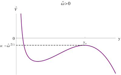
To see how the new solutions arise, we notice that in the HSC solution, the local chemical potential (3.25) vanishes asymptotically both in the UV and in the IR and admits at least one extremum value in the bulk. In the IR,

$$\hat{\mu}_{l}\sim-4\,h_{0}\,\hat{\eta}\,\hat{q}^{2}r^{\delta+1}\left(\log r\right)^{3/2}\,,\qquad r\to\infty\,.$$ (3.27)

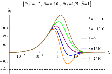
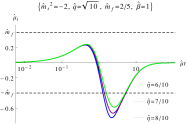
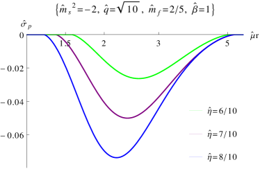
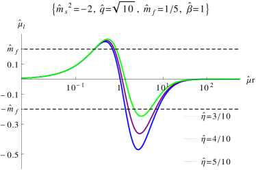
For $\hat{\eta}>0$ the local chemical potential $\hat{\mu}_{l}$ is negative in the IR for $h_{0}>0$. Moreover, since the asymptotics $\hat{\mu}_{l}\sim\hat{\mu}r$ in the UV ($r\to 0$) are not modified by $\hat{\eta}\neq 0$, $\hat{\mu}_{l}$ has both a minimum and a maximum value at finite radii in the bulk for $\hat{\eta}>0$ (see Figure 3a). For $\hat{\eta}\leq 0$, the behavior of $\hat{\mu}_{l}$ is similar to what happens in the compact star solutions of [16], where it is always positive and admits a maximum.

Similarly to the non-interacting case [16], solutions with both a non-trivial scalar and a non-trivial fluid exist when at least one local extremum of the local chemical potential in the HSC solution is larger than the mass of the fermions. Three kinds of compact star(s) solutions arise :

• Compact electron star (eCS): a fluid density is confined in a shell whose boundaries $r_{1}$ and $r_{2}$ satisfy $\hat{\mu}_{l}(r_{i})=\hat{m}_{f}$, $i=1,2$. The charge density of the fluid is positive, then the fluid is made of electrons. This situation is displayed in Figures 3a and 3b.

• Compact positron star (pCS): a fluid density is confined in a shell whose boundaries $r_{1}$ and $r_{2}$ satisfy $\hat{\mu}_{l}(r_{i})=-\hat{m}_{f}$, $i=1,2$. The charge density of the fluid is negative, then the fluid is made of positrons. This situation is displayed in Figures 4a and 4b.

• Compact positron/electron stars (peCS): In this case the solution exhibits charge polarization in the bulk: two fluid shells of opposite charges are confined in distinct regions of spacetime, bounded respectively by $(r^{e}_{1},r^{e}_{2})$ and $(r^{p}_{1},r^{p}_{2})$ determined by the equations:

  $$\hat{\mu}_{l}(r^{e}_{1})=\hat{\mu}_{l}(r^{e}_{2})=\hat{m}_{f}\,,\qquad\hat{\mu}_{l}(r^{p}_{1})=\hat{\mu}_{l}(r^{p}_{2})=-\hat{m}_{f}.$$ (3.28)

  The fluid in one region is made of electrons, the one in the other region of positrons. Clearly, for this solutions to exist, the chemical potential must change sign in the bulk. Due to fixed UV asymptotics of the local chemical potential, the fluid of electrons is situated closer to the UV boundary than the fluid of positrons.

  This situation is displayed in Figures 5a, 5b and 5c.

The kind of compact star(s) solutions that may exist depends on the maximum and minimum value of the local chemical potential,

$$\hat{\mu}_{\textnormal{max}}(\hat{m}_{s}^{2},\hat{q},\hat{m}_{f},\hat{\beta},\hat{\eta})\equiv\max_{0<r<\infty}\hat{\mu}_{l}(r)\,,\qquad\hat{\mu}_{\textnormal{min}}(\hat{m}_{s}^{2},\hat{q},\hat{m}_{f},\hat{\beta},\hat{\eta})\equiv\min_{0<r<\infty}\hat{\mu}_{l}(r)\,.$$ (3.29)

The possible outcomes are summarized in Table 1. We denote the case where no compact star(s) exists by noCS. Notice that $\hat{\mu}_{\textnormal{max}}>0$ for all $\hat{\eta}$; $\hat{\mu}_{\textnormal{min}}$ is negative when $\hat{\eta}>0$ and vanishes for $\hat{\eta}\leq 0$.

	$\hat{\mu}_{\textnormal{min}}<-\hat{m}_{f}$	$\hat{\mu}_{\textnormal{min}}>-\hat{m}_{f}$
$\hat{\mu}_{\textnormal{max}}>\hat{m}_{f}$	peCS, pCS, eCS	eCS
$\hat{\mu}_{\textnormal{max}}<\hat{m}_{f}$	pCS	noCS

Table 1: Conditions on the minimal and maximal values of the local chemical potential for the existence of the compact star(s) solutions. For given parameters, if the peCS solution exists, the pCS and eCS are also solutions to the system. “noCS” means that no compact star(s) solution exists, because $\left|\hat{\mu}_{l}(r)\right|<\hat{m}_{f}$ everywhere in the bulk.

(a)

(b)

Figure 3: Profiles of the local chemical potential (a) and the fluid charge densities (b) for eCS solutions.

(a)

(b)

Figure 4: Profiles of the local chemical potential (a) and the fluid charge densities (b) for pCS solutions.

(a)

(b)

(c)

Figure 5: Profiles of the local chemical potential (a) and the fluid charge densities (b), (c) for peCS solutions.

3.2 Phase diagrams of charged solutions

In the previous section we have seen that different arrangements of fermionic fluids are possible at zero temperature. Depending on the parameter values, we can go from the pure condensate with no fermions (holographic superconductor, or HSC), purely positive or purely negative confined fluid shells (electron or positron compact stars, or eCS and pCS respectively), and polarized shells of positive/negative charged fluid regions (compact positron-electron compact stars, or peCS). In all these configurations, the fermionic charges are surrounded by the scalar condensate, which dominates the UV and IR geometry and confines the fluid in finite regions of the bulk.

Here we address the question about which, for a given choice of parameter, is the solution that has the lowest free energy and dominates the grand-canonical ensemble. We work at zero temperature and fixed (boundary) chemical potential $\hat{\mu}$. Thus, different solutions will in general have different charge.

As was noted in [16], comparing the free energy of different solutions is relatively simple, due to the existence of a scaling symmetry of the field equations that allows to change the value of $\hat{\mu}$ within a given class of solutions. Thanks to this solution-generating symmetry, one can show that, within each class of solution, the free energy $F(\hat{\mu})$ has the simple expression

$$F_{i}(\hat{\mu})=-\frac{1}{3}c_{i}\hat{\mu}^{3}\,,$$ (3.30)

where $c_{i}$ are $\hat{\mu}$-independent constants which depend only on the class of solutions. The index $i$ runs over all solutions which exist at a given point in parameter space (HCS, eCS, pCS and/or peCS).

Equation (3.30) shows that there can be no non-trivial phase transitions between the solutions as $\hat{\mu}$ is varied. On the other hand, the constants $c_{i}$ depend non-trivially on the parameters of the model, and there can be phase transitions between different solutions as these parameters are varied.

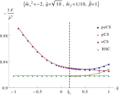
To observe the transition, it is sufficient to compute $F(\hat{\mu})$ in units of $\hat{\mu}$ for one representative of each class of solution, and for a given point in parameter space the solution with larger $c_{i}$ will be the preferred one, as $F_{i}-F_{j}\propto-(c_{i}-c_{j})\hat{\mu}^{3}$.

We performed this analysis numerically on the solutions described in the previous section. The results of this analysis reveals a rich phase diagram, with the interplay of various phase transitions.

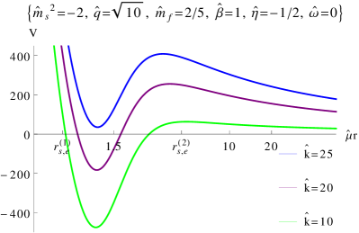
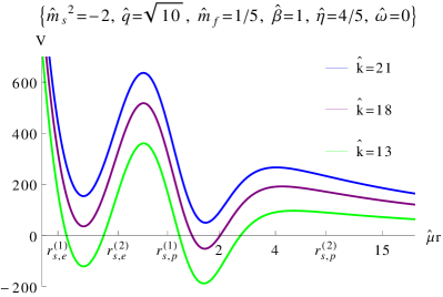
We will first analyze what happens if we vary $\hat{\eta}$ while keeping other parameters fixed (Figures 6a and 6b). As we know from [16], for $\hat{\eta}=0$, whenever compact electron star solutions exist, they dominate the ensemble. Otherwise, the preferred solution is the HSC.

Let us first choose the parameters so that, for $\hat{\eta}=0$, the compact electron star is the preferred solution (Figure 6a): if we dial up a positive interaction term $\hat{\eta}$, eventually the effect of the condensate polarizes the star and, at a critical value $\hat{\eta}_{*}>0$, we find a continuous transition to the peCS solution, which now is the one dominating the ensemble. The eCS keeps existing beyond the critical point $\hat{\eta}_{*}$, where we also see the emergence of a new pCS solution which starts dominating over the HSC solution but not over the peCS solution.

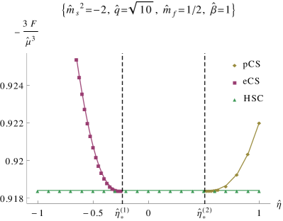
On the other hand, if we start from a point where, for $\hat{\eta}=0$, there is no eCS solution (Figure 6b), we see that dialing up $\hat{\eta}$ either way one will get to a critical point where either a positive or a negative charged star will be formed, and dominate the ensemble henceforth.

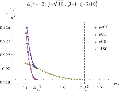
For a given (positive) value of $\hat{\eta}$, the type of solution depends on the fermion mass $\hat{m}_{f}$, as shown in Figure 6c. At small mass, the polarized peCS solution dominates over the eCS and pCS solutions. As the mass is increased, one first encounters a continuous transition from the peCS to the pCS solution at the critical value $\hat{m}_{f_{*}}^{(1)}$. At this point, the (subdominant) eCS solution merges into the (subdominant) HSC solution. Then, at the second critical point $\hat{m}_{f_{*}}^{(2)}$ the charged fluid disappears and the solution merges into the HCS solution.

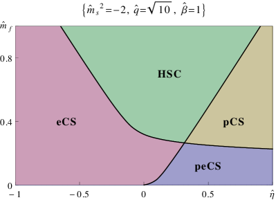
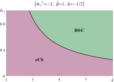
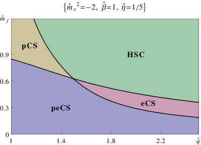
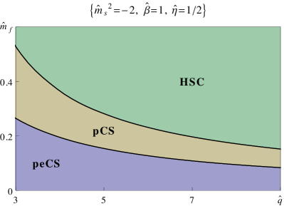
We have also analyzed the phase diagram as a function of the scalar charge $\hat{q}$. Phase diagrams of the system are displayed in Figure 7, in the plane $(\hat{m}_{f},\hat{\eta})$ at fixed scalar charge $\hat{q}$ (Figure 7a) and in the plane $(\hat{m}_{f},\hat{q})$ at fixed $\hat{\eta}$ (Figures 7b-7d). The critical lines separating the various phases correspond to the points where the maxima and minima of the local chemical potential are equal in absolute value to $\hat{m}_{f}$. The different colors correspond to the dominant phase in each region. Thus, all these transitions are continuous and take place at the points where it is possible to fill the charged fermion states: whenever a fluid solution is possible by the condition $|\hat{\mu}_{l}|>\hat{m}_{f}$, that solution will form. Furthermore, solutions in which the charge is distributed between more fluid components are preferred.

(a)

(b)

(c)

Figure 6: Free energy (normalized to the chemical potential). (a) displays the free energy as a function of $\hat{\eta}$ in the transition between eCS and peCS solutions, where $\hat{\eta}_{*}\simeq 0.17$ is the critical coupling constant. (b) displays the free energy as a function of $\hat{\eta}$ in the transition between eCS, HSC and pCS solutions; $\hat{\eta}_{*}^{(1)}\simeq-0.24$ and $\hat{\eta}_{*}^{(2)}\simeq 0.51$ are the critical coupling constants between the eCS and HSC solutions, and the HSC and pCS solutions, respectively. (c) displays the free energy as a function of $\hat{m}_{f}$ in the transition between peCS, pCS and HSC solutions; $\hat{m}_{f*}^{(1)}\simeq 0.24$ and $\hat{m}_{f*}^{(2)}\simeq 0.74$ are the critical coupling constants between the peCS and pCS solutions, and the pCS and HSC solutions, respectively. To avoid clutter, in (a), (b) and (c) we did not display the (normalized) free energy of the ES and the ERN solutions. They are much smaller than the free energy of the CS and HSC solutions : in (a) and (b), the free energy of the ES solution is equal to 0.49 and 0.42, respectively. In (c), it is between 0.41 and 0.49 depending on $\hat{m}_{f}$. In all cases, the free energy of the ERN solution is $1/\sqrt{6}\simeq 0.41$.

(a)

(b)

(c)

(d)

Figure 7: Phase diagrams of the CS/HSC transitions. The critical lines (solid black lines) correspond to the minimum and maximum values of the local chemical potential in the HSC solution, which can be seen from the plots the free energy of the different solutions (see Figure 6).

3.3 Charge distribution and screening

Let us briefly discuss how the total charge of the system is divided among the various bulk components. From the boundary field theory point of view, the only invariant definition of the charge is the total charge of the solution, that one can read off from the asymptotic behavior of the gauge field. However, it is still instructive to define, in the bulk, the separate charge of each component by the expression it would have if that were the only component present.

With the ansatz (2.4), the electric charge carried by the scalar field in the bulk is

$$\hat{Q}_{\textnormal{scalar}}=\hat{q}^{2}\int_{0}^{\infty}\mathrm{d}r\,\frac{\sqrt{g}}{r^{2}\sqrt{f}}\,h\,|\hat{\psi}|^{2}$$ (3.31)

and the electric charges of the electron and positron fluids are respectively

$$\hat{Q}_{\textnormal{e}} =\int_{r_{1}^{e}}^{r_{2}^{e}}\mathrm{d}r\,\frac{\sqrt{g}}{r^{2}}\,\hat{\sigma}_{\textnormal{e}}\,,\qquad\hat{Q}_{\textnormal{p}} =\int_{r_{1}^{p}}^{r_{2}^{p}}\mathrm{d}r\,\frac{\sqrt{g}}{r^{2}}\,\hat{\sigma}_{\textnormal{p}}\,,$$ (3.32)

where $r_{1}^{e}$ and $r_{2}^{e}$ are the boundaries of the electron star, and similarly for the positron star. The charge densities of the electron fluid $\hat{\sigma}_{\textnormal{e}}$ and the positron fluid $\hat{\sigma}_{\textnormal{p}}$ are respectively positive and negative, and they are given in Eq. (2.10) with $\hat{\mu}_{l}$ respectively positive or negative.

Additionally, due to the current-current interaction term (3.21), and the fact that by Eq. (3.22) the scalar current is linear in the gauge field, there are screening electric charges, given by

$$\hat{Q}_{\textnormal{int,e}} =-\hat{\eta}\int_{r_{1}^{e}}^{r_{2}^{e}}\mathrm{d}r\,\frac{\sqrt{g}}{r^{2}}\,\hat{q}^{2}\hat{\psi}^{2}\,\hat{\sigma}_{\textnormal{e}}\,,\qquad\hat{Q}_{\textnormal{int,p}} =-\hat{\eta}\int_{r_{1}^{p}}^{r_{2}^{p}}\mathrm{d}r\,\frac{\sqrt{g}}{r^{2}}\,\hat{q}^{2}\hat{\psi}^{2}\,\hat{\sigma}_{\textnormal{p}}\,,$$ (3.33)

which reflect the interaction between the scalar and the fluid made of electrons and positrons, respectively, and it gets contributions from the regions where the fluid density is non-vanishing.

The total electric charge of the system

$$\hat{Q}=\hat{Q}_{\textnormal{scalar}}+\left(\hat{Q}_{\textnormal{e}}+\hat{Q}_{\textnormal{int,e}}\right)+\left(\hat{Q}_{\textnormal{p}}+\hat{Q}_{\textnormal{int,p}}\right).$$ (3.34)

matches the UV asymptotic behavior of the gauge field (2.5),

$$\hat{Q}=-h^{\prime}(0)\,.$$ (3.35)

This has been verified numerically in all solutions we have constructed.

In Eq. (3.34), the second and third terms represent the total contributions from each charged fluid. Despite the possible presence of local negative charge components, we will show below that all three terms in Eq. (3.34) are positive for all solutions under considerations. This is consistent with our choice $\hat{\mu}>0$ for the boundary chemical potential in the UV asymptotics (2.5), which implies that the boundary charge, i.e. total charge of the system $\hat{Q}$ must be positive in all solutions.

Let us first consider the scalar field condensate contribution to the total charge. As a consequence of the choice $\hat{\mu}>0$ in the UV, the electric potential $h(r)$ is positive throughout the bulk. Thus, from Eq. (3.31), one can see that the electric charge of the scalar field $\hat{Q}_{\textnormal{scalar}}$ is positive.

Due to the signs of the local charge densities in (3.32), $\hat{Q}_{\textnormal{e}}$ is positive, and $\hat{Q}_{\textnormal{p}}$ is negative. However, the latter is over-screened by the scalar field through the charge of interaction $\hat{Q}_{\textnormal{int,p}}$, so that $\left(\hat{Q}_{\textnormal{p}}+\hat{Q}_{\textnormal{int,p}}\right)>0$, as can be seen from Eq. (3.32-3.33) and the fact that, inside the positron fluid, $(1-\hat{\eta}\hat{q}^{2})<0$, since by Eq. (3.25) this quantity determines the sign of the chemical potential.

By a similar reasoning, $\hat{Q}_{\textnormal{int,e}}$ is positive (negative) for $\hat{\eta}<0$ ($\hat{\eta}>0$), but $\left(\hat{Q}_{\textnormal{e}}+\hat{Q}_{\textnormal{int,e}}\right)$ is always positive. Thus, for electrons, there may be charge screening or anti-screening, but never over-screening.

Given the previous discussion, we can have a qualitative understanding of why the polarized electron-positron compact stars are stable configurations: although the positron and electron parts of the fluid are made up of positive and negative charge fermionic constituents respectively, the screening of the negative electric charge by the scalar condensate renders the total charge positive in both fluids. In particular, for peCS solutions, the two charged shells experience electromagnetic repulsion, rather than attraction. Gravitational and electromagnetic forces are competing, and this makes the solution stable.

(a)

(b)

Figure 8: Distribution of the electric charge components (a) and value of the condensate (b) in the compact star(s) solutions corresponding to the choice of parameters in Figure 6a. To avoid cluttering of the figures, the electric charge of the scalar field $\hat{Q}_{\textnormal{scalar}}$ is not displayed. . The dashed line at the critical value $\hat{\eta}_{*}\simeq 0.17$ marks the transition between the eCS and peCS visible in Figure 6a.

(a)

(b)

Figure 9: Distribution of the electric charge (a) and value of the condensate (b) in the compact star(s) solutions corresponding to Figure 6b. the vertical dashed lines indicate phase the phase transitions visible in Figure 6b: the values $\hat{\eta}_{*}^{(1)}\simeq-0.24$ and $\hat{\eta}_{*}^{(2)}\simeq 0.51$ are the critical coupling constants marking the transition between the eCS and HSC solutions, and the HSC and pCS solutions, respectively.

(a)

(b)

Figure 10: Distribution of the electric charge (a) and value of the condensate (b) in the compact star(s) solutions corresponding to Figure 6c. the The dashed lines at the critical values $\hat{m}_{f*}^{(1)}\simeq 0.24$ and $\hat{m}_{f*}^{(2)}\simeq 0.74$ mark the transitions between the peCS and pCS solutions and the pCS and HSC solutions, respectively. The same value $\hat{m}_{f*}^{(1)}$ corresponds to the (subdominant) transition between the eCS and HSC solutions

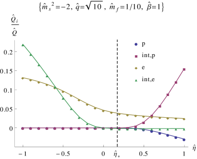
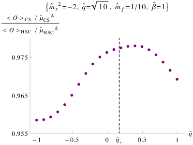
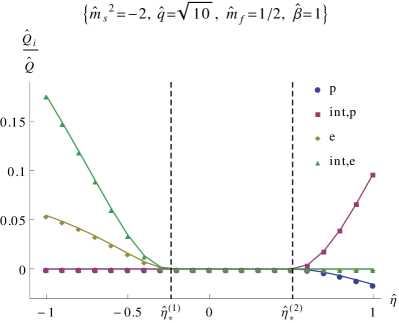
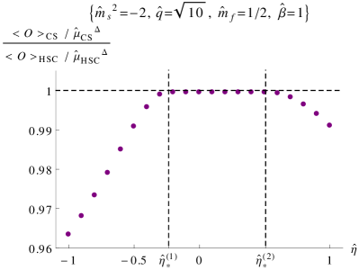
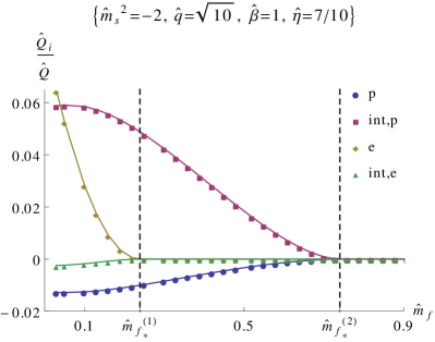
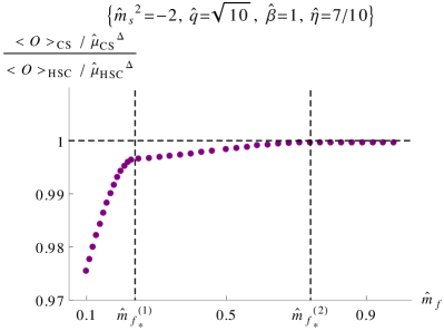
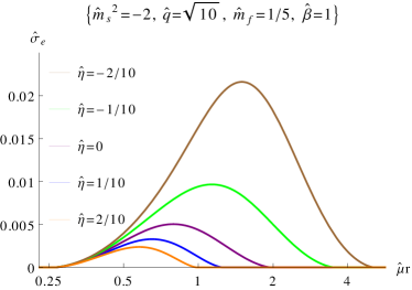
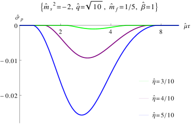
In Figures 8-10 (left) we present the distribution of the total electric charge of the system between the scalar field, the fluids of electrons and positrons and the charges of interaction for different values of the parameters (the same that were used in Figures 6a-6c). The boundary condensate $\langle\mathcal{O}\rangle$ is also shown in those figures (right). It is interesting to note that it is lower in the CS solutions than in the HSC solution. In Section 4 we will show that the presence of fermions in the bulk maps to the formation of Fermi surfaces in the dual field theory. If one interprets the scalar operator $\mathcal{O}$ as being a composite operator of the fermionic operator, decreasing of the condensate in the CS solutions can be thought of as coming from the breaking of part of the scalar operator excitations.

4 Fermionic low energy spectrum

In this section, we compute the Fermi surfaces and the fermionic low energy excitations of our model. This can be done by solving the equation of motion of a probe fermion in the WKB approximation. We assume the probe fermion is a constituent of positive charge $|q_{f}|$.

4.1 Probe fermion and the Dirac equation

The electromagnetic current of bulk elementary fermions $\chi$ with charge $|q_{f}|$ is given by

$$J_{\textnormal{ferm}}^{a}=-|q_{f}|\langle\bar{\chi}\Gamma^{a}\chi\rangle\,.$$ (4.36)

To take into account the current-current interaction between the fermions and the bosons, it is natural to add to the action for free probe fermions $\chi$ the interaction

$$S_{\textnormal{int}}=\eta\int d^{4}x\,\sqrt{-g}J_{a}^{\textnormal{ferm}}J^{a}_{\textnormal{scal}}$$ (4.37)

where $J^{a}_{\textnormal{ferm}}$ and $J^{a}_{\textnormal{scal}}$ are given by (B.141).

In Appendix B, we obtain in details the Schrödinger-like equation, but we give here the key steps. By choosing correctly the basis of Gamma matrices, the Dirac equation for a probe spinor field $\chi$ on top of the background solution can be written as an equation for the two-component spinor $\Phi=r^{-1}f^{-1/4}\chi_{1}$,

$$\left(\partial_{r}+\gamma\hat{m}_{f}g^{1/2}\sigma^{3}\right)\Phi=g^{1/2}\left\{i\gamma\sigma^{2}\left[\hat{\omega}f^{-1/2}+\hat{\mu}_{l}\right]-\gamma\hat{k}r\sigma^{1}\right\}\Phi$$ (4.38)

where we have rescaled the momentum and frequency,

$$\hat{\omega}=\frac{\omega}{\gamma}\,,\qquad\hat{k}=\frac{k}{\gamma}$$ (4.39)

by the parameter

$$\gamma\equiv\frac{|q_{f}|eL}{\kappa}\gg 1$$ (4.40)

which is large in the Thomas-Fermi approximation applied to the bulk fermions. In this limit, the Dirac equation (4.38) is equivalent to the Schrödinger-like equation

$$\Phi_{2}^{\prime\prime} =\gamma^{2}V(r)\Phi_{2}$$ (4.41)

together with the expression

$$\Phi_{1} =\frac{1}{\frac{\hat{\omega}}{\sqrt{f}}+\hat{\mu}_{l}+\hat{k}r}\left(\hat{m}_{f}\Phi_{2}-\frac{1}{\gamma}\frac{1}{\sqrt{g}}\Phi_{2}^{\prime}\right)$$ (4.42)

for the components $\Phi_{1}$ and $\Phi_{2}$ of the spinor

$$\Phi=\left(\begin{array}[]{c}\Phi_{1}\\ \Phi_{2}\end{array}\right)\,.$$ (4.45)

The potential $V(r)$ can be expressed as

$$V(r)=g(r)\left\{r^{2}\left[\hat{k}^{2}-\hat{k}_{F}^{2}(r)\right]-\frac{\hat{\omega}}{f(r)}\left[\hat{\omega}+2\sqrt{f(r)}\hat{\mu}_{l}(r)\right]\right\}+\mathcal{O}(\gamma^{-1})$$ (4.46)

where the local Fermi momentum $\hat{k}_{F}$ is defined as [21]

$$\hat{k}_{F}^{2}(r)\equiv\frac{1}{r^{2}}\left(\hat{\mu}_{l}^{2}-\hat{m}_{f}^{2}\right)\,.$$ (4.47)

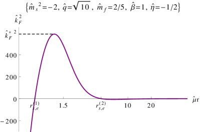
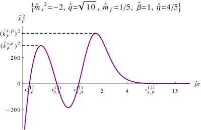
Notice that $\hat{k}_{F}^{2}>0$ inside the stars only; these are the regions where $\hat{k}_{F}$ is relevant for our considerations. The local Fermi momentum is displayed in Figure 11 for an eCS solution and a peCS solution.

(a)

(b)

Figure 11: Local Fermi momentum squared $\hat{k}_{F}^{2}(r)$ for (a) an eCS solution and (b) a peCS solution. It is positive inside the star(s) and negative outside. The points $r_{s,e}^{(1)}$, $r_{s,e}^{(2)}$, $r_{s,p}^{(1)}$ and $r_{s,p}^{(2)}$ are the boundaries of the electron and the positron stars.

The momentum $\hat{k}$ appears only through $\hat{k}^{2}$ in the potential (4.46), so we can restrict the analysis to $\hat{k}>0$ without loss of generality.

4.1.1 The Schrödinger equation in a standard form

The potential (4.46) depends on the momentum $\hat{k}$. In order to see the physical interpretation of Eq. (4.41), we put it in a Schrödinger form where $\hat{k}$ plays the role of the energy by introducing the new coordinate $y$, defined by

$$\frac{\mathrm{d}y}{\mathrm{d}r}=r\sqrt{g(r)}\,.$$ (4.48)

We then obtain the equation

$$-\partial_{y}^{2}{\varphi}+\gamma^{2}\tilde{V}(y)\varphi=-\gamma^{2}\hat{k}^{2}\varphi$$ (4.49)

for the rescaled field $\varphi\equiv r^{1/2}g^{1/4}\Phi_{2}$, where

$$\tilde{V}(y)=-\hat{k}_{F}^{2}(y)-\frac{\hat{\omega}}{r(y)^{2}f(y)}\left(\hat{\omega}+2\sqrt{f(y)}\hat{\mu}_{l}(y)\right)+\mathcal{O}\left(\gamma^{-2}\right)$$ (4.50)

in the large-$\gamma$ limit. Herein and in the following, $r(y)$ is the inverse map of

$$y(r)=\int^{r}\mathrm{d}r^{\prime}r^{\prime}\sqrt{g(r^{\prime})}\,.$$ (4.51)

Notice that $y\to\infty$ when $r\to\infty$. The equation (4.49) has to be seen as a Schrödinger equation with negative eigenvalue of the energy $E=-\gamma^{2}\hat{k}^{2}$. The potential (4.50) is now independent of the momentum $\hat{k}$.

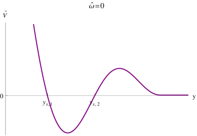
At zero frequency, the potential $\tilde{V}$ is, up to a minus sign, given by the local Fermi momentum squared (4.47). It is negative inside the star and positive outside, and the zero-energy turning points are the star boundaries where $|\hat{\mu}_{l}(y)|=\hat{m}_{f}$. Since the local chemical potential $\hat{\mu}_{l}$ vanishes in the IR as in (3.27), the local Fermi momentum behaves in this region as $\hat{k}_{F}^{2}(y)\sim-\hat{m}_{f}^{2}/r(y)^{2}$ where in the IR, the inverse map of $r(y)$ is

$$y(r)\sim\sqrt{\frac{3}{2|\hat{m}_{s}^{2}|}}\frac{r}{\sqrt{\log r}}\,,\qquad r\to\infty\,,$$ (4.52)

and the potential $\tilde{V}(y)\to 0^{+}$ at infinity. The potential $\tilde{V}$ for $\hat{\omega}=0$ is displayed schematically in Figure 12a for a compact star solution involving one star (eCS or pCS).

(a)

(b)

Figure 12: Profile of the potential of the Schrödinger equation for an eCS or a pCS solution at (a) zero frequency, (b) small frequency $0<|\hat{\omega}|\ll\hat{\mu}$. The points $y_{s,1}$ and $y_{s,2}$ are the star boundaries.

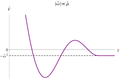
A non-zero frequency $0<|\hat{\omega}|\ll\hat{\mu}$ affects the behavior of the potential (4.50) in the near-horizon region. Indeed,

$$\tilde{V}(y)\sim-\hat{\omega}^{2}+\frac{\hat{m}_{f}^{2}}{r(y)^{2}}\,,\qquad r\to\infty\,,$$ (4.53)

so the zero-frequency limit and the near-horizon limit do not commute. This is also observed in the electron star phase [21] but with a different asymptotic behavior with respect to the potential (4.50), leading to a different conclusion as we shall see below. Outside the near-horizon region, the effects of small frequency are small and do not affect much the shape of the potential. In particular, the zero-energy turning points of the potential $\tilde{V}$ are close to the star boundaries. In the UV, the potential (4.50) behaves as

$$\tilde{V}(y)\sim\frac{\hat{m}_{f}^{2}}{y^{2}}\,,\qquad y\to 0\,,$$ (4.54)

and effects of $\hat{\omega}$ are subleading. The potential for $0<|\hat{\omega}|\ll\hat{\mu}$ is displayed in Figure 12b for a compact star solution involving one star (eCS or pCS).

Our aim is to solve the Schrödinger equation (4.49) for the field $\varphi$ to compute the poles of the retarded two-point Green function of the gauge-invariant field operator dual to the bulk fermionic particles. To do so, we shall impose the Dirichlet condition on $\varphi$ at the UV boundary and the in-falling condition in the near-horizon region. This second condition can be applied when the solution to Eq. (4.49) is oscillating in the IR, that is when $\tilde{V}(y=\infty)=-\hat{\omega}^{2}<-\hat{k}^{2}$, i.e. for $|\hat{\omega}|>\hat{k}$. The dispersion relation of the Green function corresponds in this case to quasinormal modes of the wave equation (4.49). For $|\hat{\omega}|<\hat{k}$, the solution is exponential in the near-horizon region and one shall impose the regularity condition, leading to normal modes of the equation (4.49).

The discussion of the previous paragraph allows us to distinguish three different regimes for the spectrum of the Schrödinger equation (4.49). Let us define the extremal local Fermi momentum $\hat{k}^{\star}_{F}$ by

$$\hat{k}^{\star}_{F}\equiv\max_{y_{s,1}<y<y_{s,2}}\hat{k}_{F}(y)$$ (4.55)

For $\hat{k}>\hat{k}^{\star}_{F}$, the “energy” $-k^{2}$ lies everywhere below the Schrödinger potential, and there are no eigenstates. In the intermediate region $|\hat{\omega}|<\hat{k}<\hat{k}_{F}^{\star}$, we expect to have a discrete spectrum of bound states, which are normal modes of the Schrödinger equation (4.49). Since the region of spacetime where $\tilde{V}<E$ is compact for any frequency, the number of bound states is finite at fixed frequency and is almost independent of the frequency since $\hat{\omega}\ll\hat{\mu}$ only affects the near-horizon region. For $\hat{k}<|\hat{\omega}|\ll\hat{\mu}$, the spectrum of the Schrödinger equation (4.49) is continuous but there is a discrete set of quasinormal modes, which dissipate in the IR region by quantum tunnelling. The number of quasinormal modes is finite at fixed frequency for the same reasons as for the intermediate region. By setting $\hat{\omega}=0$, one can count the number of Fermi surfaces. From the qualitative behavior of the Schrödinger potential in Figure 12a, the number of boundary Fermi momenta is finite.

In certain parameter regions, although the fluid density is non-zero, there may be no negative energy bound states (thus no Fermi surfaces): this happens for ‘small stars’, for which the potential $\tilde{V}$ is not deep enough inside the star to allow any bound state.

We then expect to obtain a finite number of boundary Fermi momenta $\hat{k}_{n}$ ($n=0,\dots,N-1$) satisfying $\hat{k}_{n}<\hat{k}_{F}^{\star}$ in the large-$\gamma$ limit. Each boundary Fermi surface admits particle excitations which are stable at small energy $|\hat{\omega}|<\hat{k}$. At larger frequency $|\hat{\omega}|>\hat{k}$ with $|\hat{\omega}|\ll\hat{\mu}$, the excitations are resonances, they can dissipate. This dissipation maps in the bulk to the possible quantum tunnelling of the modes into the near-horizon region. The modes dissipate only at sufficiently large frequency due to the fact that the compact star does not occupy the inner region of the bulk spacetime. From the field theory point of view, the bosonic modes, represented in the bulk by the scalar field, the metric and the gauge field, do not interact with the fermions at sufficiently low energy and the excitations around the $n$-th Fermi surface are stable up to $|\hat{\omega}|\sim\hat{k}_{n}$.

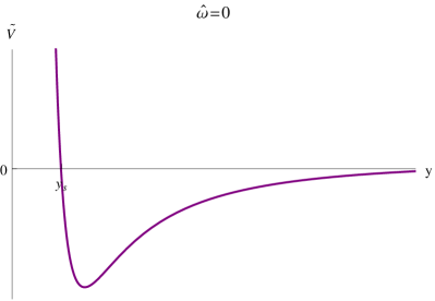
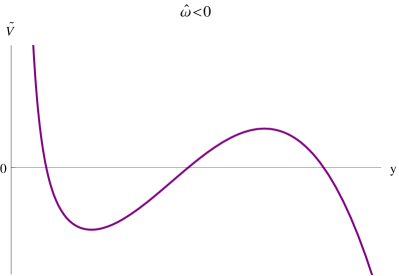
Let us compare the situation to the electron star phase, studied in detail in [21]. At zero frequency the potential is negative for $y>y_{s}$, where $y_{s}$ is the star boundary, and $\tilde{V}(y)\to 0^{-}$ for $y\to\infty$. For $\hat{\omega}\neq 0$, the potential diverges to $-\infty$ in the IR so dissipation occurs for any non-zero frequency. This is because the fluid does occupy the inner region of spacetime and the boundary fermions interact with the bosonic modes at low energy. For $\hat{\omega}>0$, the potential admits a local maximum at a point $y_{\star}\propto\hat{\omega}^{-1/z}$ where $\tilde{V}(y_{\star})\propto-\hat{\omega}^{2/z}<0$. The constant of proportionality can be easily computed analytically. From the Schrödinger equation (4.49), it means that for positive frequency, the modes are unstable for $\hat{\omega}>\hat{k}^{z}$ because, as explained in [21], the fermionic excitations strongly interact with the critical modes of the Lifshitz sector. On the other hand, for $\hat{\omega}<0$, the potential admits two turning points in the Lifshitz region, so there is a region where it is positive. The conclusion is that there is no strong dissipation and one finds a set of quasinormal modes for all $\hat{k}\lesssim\hat{k}_{F}^{\star}$ [21]. These situations are displayed in Figure 13.

(a)

(b)

(c)

Figure 13: Profile of the potential of the Schrödinger equation in the electron star phase at, (a) zero frequency, (b) negative frequency and (c) positive frequency. The point $y_{s}$ is the star boundary and $y_{\star}$ is the point where $\tilde{V}$ admits a local maximum in the Lifshitz region for $\hat{\omega}<0$.

We should notice that for the compact star solutions, $\tilde{V}$ also admits a local maximum, as shown in Figure 12. However, this local maximum is positive at zero frequency and not modified at small frequency $|\hat{\omega}|\ll\hat{\mu}$ because it does not belong to the asymptotic IR region. At larger frequencies, the effects of $\hat{\omega}$ are also relevant outside the near-horizon region. It may happen that for sufficiently large frequencies, this local maximum becomes negative. In this case, the potential would be negative for all $y$ larger than the first turning point, leading to unstable states at small momentum.

We have argued above that the number of boundary Fermi momenta dual to the compact star solutions is finite. In the electron star phase on the other hand, at zero frequency we see from (2.18) that the potential asymptotes to zero in the IR as

$$\tilde{V}(y)\sim-\frac{g_{\infty}\left(h_{\infty}^{2}-\hat{m}_{f}^{2}\right)}{y^{2}}\,,\qquad y\to\infty\,.$$ (4.56)

It means that there is accumulation of levels at small momentum and, as we will explicitly show in Section4.6, the number of Fermi surfaces turns out to be infinite [26].

Here, we focus on the regime $|\hat{\omega}|<\hat{k}$ with $|\hat{\omega}|\ll\hat{\mu}$. In this case, all the modes are bound states. We leave the detailed study of the case $|\hat{\omega}|>\hat{k}$ for future considerations [27].

4.1.2 Bound states for $|\hat{\omega}|\ll\hat{k}$

In the electron star phase, the dispersion relation of the fermionic excitations around the Fermi surfaces was found to be linear, up to a (imaginary) dissipative term [21]. We will see later that this is also what we obtain for the compact star phases. In the rest of this paper, we will be interested in the behavior of the particle excitations close to the Fermi surfaces, that is for $|\hat{\omega}|\sim|\hat{k}_{n}-\hat{k}|\ll\hat{k}_{n}$. In this case, $|\hat{\omega}|\ll\hat{k}$ and the dependence on $\hat{\omega}$ of the potential (4.50) can be neglected everywhere, in particular in the IR region, and one can consistently set $\hat{\omega}=0$. The potential is then simply given by

$$\tilde{V}(y)=-\hat{k}_{F}^{2}(y)\,.$$ (4.57)

It is easy to generalize the above discussion to peCS solutions. In Figure 11, we display the local Fermi momentum for an eCS solution and a peCS solution. For convenience, we plot it in the original variable $r$. Doing so does not affect the analysis as it only changes the shape of the local Fermi momentum in the radial direction and does not modify the extremal values of it. It is clear from (4.49) that for $\hat{k}>\hat{k}_{F}(r)$, the solution is exponential while it is oscillating for $\hat{k}<\hat{k}_{F}(r)$. There can exist zero, one or two regions where $\hat{k}<\hat{k}_{F}(r)$ depending on the background solution and the value of $\hat{k}$ compared to the local maxima of $\hat{k}_{F}$. For eCS and pCS solutions, the extremal local Fermi momentum is

$$\hat{k}^{\star}_{F}\equiv\max_{r_{s}^{(1)}<r<r_{s}^{(2)}}\hat{k}_{F}(r)$$ (4.58)

and for peCS solutions, there exist two local extrema

$$\hat{k}_{F}^{\star,p}\equiv\max_{r_{s,p}^{(1)}<r<r_{s,p}^{(2)}}\hat{k}_{F}(r)\qquad\textnormal{and}\qquad\hat{k}_{F}^{\star,e}\equiv\max_{r_{s,e}^{(1)}<r<r_{s,e}^{(2)}}\hat{k}_{F}(r)\,.$$ (4.59)

The bounds in the maxima are the star boundaries of the star(s) of the different solutions. The conditions for oscillations are detailed in Table 2.

	eCS/pCS	peCS
$\hat{k}<\hat{k}_{F}^{\star}$	oscillations	$\times$
$\hat{k}_{F}^{\star}<\hat{k}$	no oscillations	$\times$
$\hat{k}<\hat{k}_{F}^{\star,e}$ and $\hat{k}<\hat{k}_{F}^{\star,p}$	$\times$	oscillations in electron and positron stars
$\hat{k}_{F}^{\star,e}<\hat{k}<\hat{k}_{F}^{\star,p}$	$\times$	oscillations in positron star
$\hat{k}_{F}^{\star,p}<\hat{k}<\hat{k}_{F}^{\star,e}$	$\times$	oscillations in electron star
$\hat{k}_{F}^{\star,p}<\hat{k}$ and $\hat{k}_{F}^{\star,e}<\hat{k}$	$\times$	no oscillations

Table 2: Conditions on the momentum for oscillations. When possible, oscillations occur in the region(s), located in the star(s), where $\hat{k}<\hat{k}_{F}(r)$.

When oscillations can occur, as discussed above we expect in the large-$\gamma$ limit that we are considering to obtain a finite number of eigenvalues $k_{n}$, bounded above by the extremal local Fermi momenta. They correspond to oscillations which are localized in the star for pCS and eCS solutions. For peCS solutions, for $\min(\hat{k}_{F}^{\star,p},\hat{k}_{F}^{\star,e})<\hat{k}<\max(\hat{k}_{F}^{\star,p},\hat{k}_{F}^{\star,e})$ these oscillations are localized in one of the two stars while for smaller momentum there can be quantum tunnelling between the two stars.

4.2 The WKB analysis for $|\hat{\omega}|\ll\hat{k}<\hat{k}_{F}^{\star}$

Even if the Schrödinger problem in the standard form allows to have a clear analysis of the spectrum, we can equivalently obtain the Green function for $\hat{k}<\hat{k}_{F}^{\star}$ from the original Schrödinger-like equation (4.41) with potential (4.46) by looking for zero-energy solutions. As noticed above, the parameter $\gamma$ defined by (4.40) is large,

$$\gamma\gg 1\,.$$ (4.60)

This allows us to solve Eq. (4.41) for $\hat{k}<\hat{k}_{F}^{\star}$ by applying the WKB approximation if the conditions [21]

$$|V^{\prime}(r)|\ll\gamma|V(r)|^{3/2}\qquad\textnormal{and}\qquad|V^{\prime\prime}(r)|\ll\gamma^{2}|V(r)|^{2}$$ (4.61)

are satisfied. This is the case if the momentum $\hat{k}$ is not too close to the local extremal Fermi momenta (4.58) and (4.59). This means in particular that the potential vanishes linearly at the turning points.

The potential (4.46) is positive both in the UV and the IR, where it behaves as

$$V\sim\frac{\hat{m}_{f}^{2}}{r^{2}}\,,\qquad r\sim 0\,,$$ (4.62)

and

$$V\sim\frac{3}{2|\hat{m}_{s}^{2}|}\frac{\hat{k}^{2}}{\log r}\,,\qquad r\sim\infty\,,$$ (4.63)

where we have used the fact that $|\hat{\omega}|\ll\hat{k}$. As explained in the previous section, for $\hat{k}<\hat{k}_{F}^{\star}$ there can be one or two regions where $V<0$; in these regions, the solution is oscillating and we expect to observe bound states. In Figure 14, we display these possible situations by plotting the potential (4.46) for the compact star(s) solutions at zero frequency and several values of the momentum.

(a)

(b)

Figure 14: Profiles of the potential (4.46) at zero frequency. (a) The potential for an eCS solutions. The extremal Fermi momentum is in this case $\hat{k}_{F}^{\star}\simeq 24.3$. (b) The potential for a peCS solution. The extremal Fermi momenta are $\hat{k}_{F}^{\star,e}\simeq 17.0$ and $\hat{k}_{F}^{\star,p}\simeq 19.6$. In (a) and (b), the points $r_{s,e}^{(1)}$, $r_{s,e}^{(2)}$, $r_{s,p}^{(1)}$ and $r_{s,p}^{(2)}$ are the boundaries of the electron and the positron stars.

To get the Green function of the gauge-invariant fermionic operators dual to the probe bulk fermion $\chi$, we shall relate the UV asymptotics of $\Phi$ with the normalizable and non-normalizable modes of $\chi$. In the UV ($r\to 0$), the asymptotic solution to the bulk Dirac equation (4.38) is [28]

$$\Phi\simeq A(\hat{k},\hat{\omega})\,r^{-\gamma\hat{m}_{f}}\left[\left(\begin{array}[]{c}1\\ 0\end{array}\right)+\dots\right]+B(\hat{k},\hat{\omega})\,r^{\gamma\hat{m}_{f}}\left[\left(\begin{array}[]{c}0\\ 1\end{array}\right)+\dots\right]$$ (4.68)

where $A$ and $B$ are independent of the radial coordinate. The Green function of the fermionic operator dual to the bulk spinor $\Phi$ is then given by

$$G^{R}(\hat{k},\hat{\omega})=\frac{B(\hat{k},\hat{\omega})}{A(\hat{k},\hat{\omega})}\,.$$ (4.69)

As shown in Appendix C, $\Phi_{2}$ behaves in the UV as

$$\Phi_{2}(r)\simeq a_{+}^{\epsilon}(\hat{k},\hat{\omega})\left(\frac{r}{\epsilon}\right)^{\gamma\hat{m}_{f}}+a_{-}^{\epsilon}(\hat{k},\hat{\omega})\left(\frac{r}{\epsilon}\right)^{-\gamma\hat{m}_{f}+1}\,,$$ (4.70)

where $\epsilon\ll 1$ is a UV cut-off. Matching this solution with (4.68), the Green function is fully expressed in terms of the UV asymptotics of the scalar field $\Phi_{2}$ as

$$G^{R}(\hat{k},\hat{\omega})=\frac{\hat{\mu}+\hat{\omega}+\hat{k}}{2\hat{m}_{f}}\lim_{\epsilon\to 0}\frac{a_{+}^{\epsilon}(\hat{k},\hat{\omega})}{a_{-}^{\epsilon}(\hat{k},\hat{\omega})}\epsilon^{-2\gamma\hat{m}_{f}}\,.$$ (4.71)

Notice that the functions $a_{+}^{\epsilon}(\hat{k},\hat{\omega})$ and $a_{-}^{\epsilon}(\hat{k},\hat{\omega})$ depend on the UV cutoff $\epsilon$.

To obtain the ratio $a_{+}^{\epsilon}(\hat{k},\hat{\omega})/a_{-}^{\epsilon}(\hat{k},\hat{\omega})$ in Eq. (4.71), we must impose normalizability of the wave function in the IR and integrate out Eq. (4.41) from IR to UV. This can be done in the WKB approximation with large parameter $\gamma$. The details of the computation are given in Appendix C. The general form of the Green function is

$$G_{R}(\hat{k},\hat{\omega})=\frac{\hat{\mu}+\hat{\omega}+\hat{k}}{2\hat{m}_{f}}\,\mathcal{G}(\hat{k},\hat{\omega})\,\lim_{r\to 0}r^{-2\gamma\hat{m}_{f}}\exp\left[-2\gamma\int_{r}^{r_{1}}\mathrm{d}s\sqrt{V(s)}\right]\,.$$ (4.72)

Here, $r_{1}$ is the turning point of the potential $V$ the closest to the UV boundary. The exponential suppression is due to the fact that the potential is large close to the boundary; the fermion has to tunnel into the spacetime. The function $\mathcal{G}(\hat{k},\hat{\omega})$ depends on the behavior of the potential $V$ at momentum $\hat{k}$ and frequency $\hat{\omega}$.

4.3 The Green function for eCS and pCS solutions

For eCS and pCS solutions, the Green function has poles when $V<0$ in one region. In this case, we find in Appendix C that

$$\mathcal{G}(\hat{k},\hat{\omega})=\frac{1}{2}\tan W(\hat{k},\hat{\omega})$$ (4.73)

where

$$W(\hat{k},\hat{\omega})=\gamma\int_{r_{1}}^{r_{2}}\mathrm{d}r\sqrt{|V(r)|}\,.$$ (4.74)

The two points $r_{1}$ and $r_{2}$ ($r_{1}<r_{2}$) are the turning points of the potential $V$.

The poles of the Green function are situated at

$$W(\hat{k},\hat{\omega})=\frac{\pi}{2}+n\pi\,,\quad n\in\mathbb{N}\,.$$ (4.75)

This equation defines $N$ boundary Fermi momenta $\hat{k}=\hat{k}_{n}$, where $n=0,\dots,N-1$, satisfying

$$0<\hat{k}_{N-1}<\dots<\hat{k}_{0}<\hat{k}_{F}^{\star}\,.$$ (4.76)

Since $\gamma\gg 1$, the number $N$ of boundary Fermi momenta is large and the WKB analysis is reliable for large $n$. By computing explicitly the normal modes of the equation (4.41), we have verified that the poles of the Green function are well-approximated by the WKB analysis. Expanding (4.73) around the poles (4.75), we obtain the Green function

$$G^{R}(\hat{k},\hat{\omega})=\frac{\hat{\mu}+\hat{\omega}+\hat{k}}{2\hat{m}_{f}}\sum_{0<\hat{k}_{n}<\hat{k}_{F}^{\star}}\frac{\gamma^{-1}c_{n}e^{-2\gamma a_{n}}}{\hat{\omega}-v_{n}(\hat{k}-\hat{k}_{n})}$$ (4.77)

where

$$v_{n} =-\frac{\partial_{\hat{k}}\,W(\hat{k}_{n},0)}{\partial_{\hat{\omega}}\,W(\hat{k}_{n},0)}\,,\qquad c_{n}=-\frac{\gamma}{2}\left[\partial_{\hat{\omega}}W(\hat{k}_{n},0)\right]^{-1},$$ (4.78)

$$a_{n} =\int_{0}^{r_{1}}\mathrm{d}r\sqrt{V(\hat{k}_{n},0)}+\hat{m}_{f}\log r_{1}\,.$$ (4.79)

Notice that $v_{n}>0$ for eCS and $v_{n}<0$ for pCS which means that, as expected, the electron star and the positron star form respectively electronic and positronic Fermi surfaces in the dual field theory.

4.4 The Green function for peCS solutions

For peCS solutions, the Green function has poles of the same kind as for the eCS and the pCS solutions for intermediate momentum. Indeed, these boundary Fermi momenta $\hat{k}_{n}$ are bounded as

$$\hat{k}_{F}^{\star,e}<\hat{k}_{N-1}<\dots<\hat{k}_{0}<\hat{k}_{F}^{\star,p}$$ (4.80)

where the oscillations happen in the positron star and vice-versa when they happen in the electron star. Moreover, for small momentum, $V<0$ in two regions and, as shown in Appendix C, the Green function reads

$$\mathcal{G}(\hat{k},\hat{\omega})=\frac{4e^{2X}\sin Y\cos Z+\cos Y\sin Z}{8e^{2X}\cos Y\cos Z-2\sin Y\sin Z}$$ (4.81)

where

$$X(\hat{k},\hat{\omega}) =\gamma\int_{r_{2}}^{r_{3}}\mathrm{d}r\sqrt{V(r)}\,,\qquad Y(\hat{k},\hat{\omega})=\gamma\int_{r_{1}}^{r_{2}}\mathrm{d}r\sqrt{|V(r)|}\,,$$ (4.82)

$$Z(\hat{k},\hat{\omega}) =\gamma\int_{r_{3}}^{r_{4}}\mathrm{d}r\sqrt{|V(r)|}\,.$$ (4.83)

The potential $V$ vanishes linearly at the turning points $r_{1}<r_{2}<r_{3}<r_{4}$. From (4.81) we see that the conditions for $\mathcal{G}$ to have a pole are

$$(Y,Z)=\left(\frac{\pi}{2}+n\pi,m\pi\right)\quad\textnormal{and}\quad(Y,Z)=\left(n\pi,\frac{\pi}{2}+m\pi\right)\,,\quad n,m\in\mathbb{N}$$ (4.84)

for all $X$, and

$$e^{2X}=\frac{1}{4}\tan Y\tan Z\,,\qquad\tan Y\tan Z\geq 0\,.$$ (4.85)

However the conditions  (4.84) are generically not satisfied for any pair $\{\hat{k},\hat{\omega}\}$ and so they do not give rise to poles.

The boundary Fermi momenta $\hat{k}_{\bar{n}}$ are then found by solving  (4.85) at zero frequency. Around $\hat{k}=\hat{k}_{\bar{n}}$ and $\hat{\omega}=0$, (4.81) becomes

$$\mathcal{G}(\hat{k},\hat{\omega})\simeq\frac{\gamma^{-1}c_{\bar{n}}}{\hat{\omega}-v_{\bar{n}}(\hat{k}-\hat{k}_{\bar{n}})}$$ (4.86)

where

$$v_{\bar{n}}=-\frac{8\,e^{2X_{\bar{n}}}\,\partial_{\hat{k}}X_{\bar{n}}-\frac{\tan Z_{\bar{n}}}{\cos^{2}Y_{\bar{n}}}\,\partial_{\hat{k}}Y_{\bar{n}}-\frac{\tan Y_{\bar{n}}}{\cos^{2}Z_{\bar{n}}}\,\partial_{\hat{k}}Z_{\bar{n}}}{8\,e^{2X_{\bar{n}}}\,\partial_{\hat{\omega}}X_{\bar{n}}-\frac{\tan Z_{\bar{n}}}{\cos^{2}Y_{\bar{n}}}\,\partial_{\hat{\omega}}Y_{\bar{n}}-\frac{\tan Y_{\bar{n}}}{\cos^{2}Z_{\bar{n}}}\,\partial_{\hat{\omega}}Z_{\bar{n}}}$$ (4.87)

and

$$c_{\bar{n}}=\gamma\tan Z_{\bar{n}}\left(1+\tan^{2}Y_{\bar{n}}\right)\left[16\,e^{2X_{\bar{n}}}\,\partial_{\hat{\omega}}X_{\bar{n}}-2\frac{\tan Z_{\bar{n}}}{\cos^{2}Y_{\bar{n}}}\,\partial_{\hat{\omega}}Y_{\bar{n}}-2\frac{\tan Y_{\bar{n}}}{\cos^{2}Z_{\bar{n}}}\,\partial_{\hat{\omega}}Z_{\bar{n}}\right]^{-1}$$ (4.88)

with

$$X_{\bar{n}}\equiv X(\hat{k}_{\bar{n}},0)$$ (4.89)

and similarly for $Y$ and $Z$.

The Green function for peCS solutions with $\hat{k}_{F}^{\star,e}<\hat{k}_{F}^{\star,p}$ can therefore be written as

$$G^{R}(\hat{k},\hat{\omega})=\frac{\hat{\mu}+\hat{\omega}+\hat{k}}{2\hat{m}_{f}} \left(\sum_{\hat{k}_{F}^{\star,e}<\hat{k}_{n}^{Z}<\hat{k}_{F}^{\star,p}}\frac{\gamma^{-1}c_{n}^{Z}e^{-2\gamma a_{n}^{Z}}}{\hat{\omega}-v_{n}^{Z}(\hat{k}-\hat{k}_{n}^{Z})}+\sum_{0<\hat{k}_{\bar{n}}<\hat{k}_{F}^{\star,e}}\frac{\gamma^{-1}c_{\bar{n}}e^{-2\gamma a_{\bar{n}}}}{\hat{\omega}-v_{\bar{n}}(\hat{k}-\hat{k}_{\bar{n}})}\right)$$ (4.90)

where

$$v_{n}^{Z} =-\frac{\partial_{\hat{k}}\,Z(\hat{k}_{n}^{Z},0)}{\partial_{\hat{\omega}}\,Z(\hat{k}_{n}^{Z},0)}\,,\qquad c_{n}^{Z}=-\frac{\gamma}{2}\left[\partial_{\hat{\omega}}Z(\hat{k}_{n}^{Z},0)\right]^{-1},$$ (4.91a)

$$a_{n}^{Z} =\int_{0}^{r_{1}}\mathrm{d}r\sqrt{V(\hat{k}_{n}^{Z},0)}+\hat{m}_{f}\log r_{1}\,.$$ (4.91b)

We have denoted by $\hat{k}_{n}^{Z}$ the boundary Fermi momenta obtained when the potential $V$ is negative in one region; in this case we have $Z(\hat{k}_{n}^{Z},0)=\pi/2+n\pi$. When $\hat{k}_{F}^{\star,p}<\hat{k}_{F}^{\star,e}$, the Green function for peCS solutions is

$$G^{R}(\hat{k},\hat{\omega})=\frac{\hat{\mu}+\hat{\omega}+\hat{k}}{2\hat{m}_{f}} \left(\sum_{\hat{k}_{F}^{\star,p}<\hat{k}_{n}^{Y}<\hat{k}_{F}^{\star,e}}\frac{\gamma^{-1}c_{n}^{Y}e^{-2\gamma a_{n}^{Y}}}{\hat{\omega}-v_{n}^{Y}(\hat{k}-\hat{k}_{n}^{Y})}+\sum_{0<\hat{k}_{\bar{n}}<\hat{k}_{F}^{\star,p}}\frac{\gamma^{-1}c_{\bar{n}}e^{-2\gamma a_{\bar{n}}}}{\hat{\omega}-v_{\bar{n}}(\hat{k}-\hat{k}_{\bar{n}})}\right)$$ (4.92)

where $v_{n}^{Y}$, $c_{n}^{Y}$ and $a_{n}^{Y}$ are defined by (4.91) where one has to replace $Z$ by $Y$.

(a)

(b)

(c)

(d)

Figure 15: Poles of $\mathcal{G}$ for peCS solutions in the (Y-Z)-plan for different values of $X$.

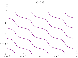
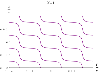
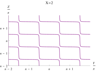
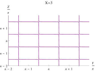
In Figure 15, we display the poles of (4.81) in the $(Y,Z)$-plan for constant values of $X$. We see that in the large-$\gamma$ limit, the location of the poles of (4.81) are well-approximated by

$$(Y,Z)\simeq\left(\frac{\pi}{2}+n\pi,Z\right)\quad\textnormal{and}\quad(Y,Z)\simeq\left(Y,\frac{\pi}{2}+m\pi\right)\,,\qquad n,m\in\mathbb{N}\,.$$ (4.93)

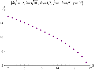
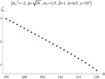
as suggested by Figure 15d. We denote by $\hat{k}_{\bar{n}}^{Y}$ and $\hat{k}_{\bar{m}}^{Z}$ the boundary Fermi momenta corresponding to the poles (4.93) and computed in the WKB approximation. In Figure 16 we give them for a peCS solution. These poles match with a high accuracy to the normal modes of the Schrödinger-like equation (4.41) that we have computed explicitly.

(a)

(b)

Figure 16: Boundary Fermi momenta for a peCS solution. The $\hat{k}_{\bar{n}}^{Y}$’s and the $\hat{k}_{\bar{m}}^{Z}$’s are the Fermi momenta of electron-like and hole-like Fermi surfaces in the dual field theory, respectively.

4.5 The Luttinger count

The Luttinger theorem relates the total charge of a Fermi liquid to the volume enclosed in the Fermi surface. For spin-$1/2$ particles with charge $|q_{f}|$ in two spatial dimensions, the Luttinger count is [29]

$$Q_{\textnormal{FS}}=|q_{f}|\sum_{i}\frac{2}{(2\pi)^{2}}V_{i}\,,$$ (4.94)

where $V_{i}$ are the volumes of the Fermi surfaces, given by $V_{i}=\pi p_{i}^{2}$ where $p_{i}$ is the Fermi momentum of the $i$-th Fermi surface. In the WKB approximation, one can approximate the discrete sum in (4.94) by an integral [21]; for eCS and pCS solutions we have

$$\sum_{i}\frac{1}{2\pi}p_{i}^{2}=\sum_{n}\frac{1}{2\pi}k_{n}^{2}=\frac{1}{2\pi}\int_{0}^{{k_{F}^{\star}}^{2}}\mathrm{d}E\,E\int_{r_{1}}^{r_{2}}\mathrm{d}r\,r\sqrt{g}\frac{1}{\sqrt{k_{F}^{2}-E}}$$ (4.95)

where the Fermi momenta $k_{n}$ appear (with hats) in the Green function (4.77). This leads to the relations [21]

$$|q_{f}|\sum_{n}\frac{1}{2\pi}k_{n}^{2}=Q_{\textnormal{e}}\,,$$ (4.96a)

$$-|q_{f}|\sum_{n}\frac{1}{2\pi}k_{n}^{2}=Q_{\textnormal{p}}\,,$$ (4.96b)

for eCS and pCS solutions, respectively, where the charges $Q_{e}$ and $Q_{p}$ are defined in Section 3. It means that as expected, the eCS and pCS solutions admit respectively boundary electronic and positronic Fermi surfaces. This is consistent with the fact that the particle excitations are electronic in the field theory dual to the eCS solution and positronic in the field theory dual to the pCS solution. The Luttinger relation is

$$|q_{f}|\sum_{i}\frac{1}{2\pi}p_{i}^{2}=Q-Q_{\textnormal{scalar}}-Q_{\textnormal{int,e}}$$ (4.97)

for eCS solutions and

$$-|q_{f}|\sum_{i}\frac{1}{2\pi}p_{i}^{2}=Q-Q_{\textnormal{scalar}}-Q_{\textnormal{int,p}}$$ (4.98)

for pCS solutions. These situations are similar to the fractionalized phases of [6]; here the bosonic field takes the role of the charged event horizon, and there is also screening of the fermionic charge by the condensate.

For peCS solutions, the Luttinger count is

$$Q_{\textnormal{FS}}^{\textnormal{e}}=|q_{f}|\sum_{i}\frac{1}{2\pi}(p_{i}^{e})^{2}+|q_{f}|\sum_{j}\frac{1}{2\pi}(q_{j}^{e})^{2}$$ (4.99)

for electronic Fermi surfaces and

$$Q_{\textnormal{FS}}^{\textnormal{p}}=-|q_{f}|\sum_{i}\frac{1}{2\pi}(p_{i}^{p})^{2}-|q_{f}|\sum_{j}\frac{1}{2\pi}(q_{j}^{p})^{2}$$ (4.100)

for positronic Fermi surfaces. Here, $p_{i}^{e}$ and $q_{j}^{e}$ denote the boundary Fermi momenta of electronic Fermi surfaces corresponding to the cases where the potential $V$ is negative in one and two regions respectively in the bulk, and similarly for positrons. For $\hat{k}_{F}^{\star,e}<\hat{k}_{F}^{\star,p}$, we have

$$|q_{f}|\sum_{i}\frac{1}{2\pi}(p_{i}^{e})^{2} =0\,,$$ (4.101a)

$$|q_{f}|\sum_{j}\frac{1}{2\pi}(q_{j}^{e})^{2} =|q_{f}|\sum_{\bar{n}}\frac{1}{2\pi}(k_{\bar{n}}^{Y})^{2}=\frac{|q_{f}|}{2\pi}\int_{0}^{({k_{F}^{\star,e}})^{2}}\mathrm{d}E\,E\int_{r_{1}}^{r_{2}}\mathrm{d}r\,r\sqrt{g}\frac{1}{\sqrt{k_{F}^{2}-E}}\,,$$ (4.101b)

$$-|q_{f}|\sum_{i}\frac{1}{2\pi}(p_{i}^{p})^{2} =-|q_{f}|\sum_{n}\frac{1}{2\pi}(k_{n}^{Z})^{2}=-\frac{|q_{f}|}{2\pi}\int_{{(k_{F}^{\star,e})}^{2}}^{{(k_{F}^{\star,p})}^{2}}\mathrm{d}E\,E\int_{r_{3}}^{r_{4}}\mathrm{d}r\,r\sqrt{g}\frac{1}{\sqrt{k_{F}^{2}-E}}\,,$$ (4.101c)

$$-|q_{f}|\sum_{j}\frac{1}{2\pi}(q_{j}^{p})^{2} =-|q_{f}|\sum_{\bar{n}}\frac{1}{2\pi}(k_{\bar{n}}^{Z})^{2}=-\frac{|q_{f}|}{2\pi}\int_{0}^{({k_{F}^{\star,e}})^{2}}\mathrm{d}E\,E\int_{r_{3}}^{r_{4}}\mathrm{d}r\,r\sqrt{g}\frac{1}{\sqrt{k_{F}^{2}-E}}\,.$$ (4.101d)

We conclude that

$$Q_{\textnormal{FS}}^{\textnormal{e}}=Q_{\textnormal{e}}\qquad\textnormal{and}\qquad Q_{\textnormal{FS}}^{\textnormal{p}}=Q_{\textnormal{p}}\,.$$ (4.102)

This result is also valid when $\hat{k}_{F}^{\star,p}<\hat{k}_{F}^{\star,e}$. So we have

$$Q_{\textnormal{FS}}^{\textnormal{e}}+Q_{\textnormal{FS}}^{\textnormal{p}}=Q-Q_{\textnormal{scalar}}-Q_{\textnormal{int,e}}-Q_{\textnormal{int,p}}\,.$$ (4.103)

Thus, we have shown that the charge that one can assign to fermionic fluid components (which does not include the effect of screening due to the scalar field) is reproduced by the total volume of particle-like and hole-like Fermi surfaces via the Luttinger count.

4.6 Fermi surfaces and phase transitions

We have shown in the previous sections that the compact star solutions exhibit a large number of boundary Fermi surfaces when the WKB approximation is applicable. Since the field theory is rotationally invariant, they are circular and each of them is specified by a Fermi momentum $\hat{k}_{n}$, which lie between zero and the maximal value $\hat{k}^{\star}_{F}$.

In the WKB approximation, the number of Fermi surfaces with Fermi momentum in the interval $(\hat{k},\hat{k}_{F}^{\star})$ of a solution with one star – eCS, pCS or ES – is given by the integral [26]:

$$N(\hat{k},\hat{k}_{F}^{\star})\propto\gamma\int_{y_{1}}^{y_{2}}\mathrm{d}y\,\sqrt{\hat{k}_{F}^{2}(y)-\hat{k}^{2}}$$ (4.104)

where $y_{1}$ and $y_{2}$ are boundaries of the region where $\hat{k}_{F}^{2}(y)>\hat{k}^{2}$. The total number of Fermi surfaces $N$ is then

$$N\propto\gamma\int_{y_{s,1}}^{y_{s,2}}\mathrm{d}y\,\hat{k}_{F}(y)$$ (4.105)

where $y_{s,1}$ and $y_{s,2}$ are the star boundaries. This formula is in fact not exact, because for $\hat{k}$ close to $\hat{k}_{F}^{\star}$, the WKB approximation is not valid. However, the contribution of such momenta to the total number of levels is small, and non-vanishing, for eCS, pCS and ES solutions. For the eCS and pCS solutions, the star boundaries $y_{s,1}$ and $y_{s,2}$ are finite, so the total number of Fermi surfaces is finite; this also applies to the peCS solutions. The corresponding Fermi momenta are bounded by zero and the extremal local Fermi momenta.

For the (unbounded) electron star solution, the total number of Fermi surfaces (4.105) can be written as

$$N\propto\gamma\int_{y_{s}}^{y_{0}}\mathrm{d}y\,\hat{k}_{F}(y)+\gamma\int_{y_{0}}^{\infty}\mathrm{d}y\,\frac{\sqrt{g_{\infty}(h_{\infty}^{2}-\hat{m}_{f}^{2})}}{y}$$ (4.106)

where $y_{s}$ is the star boundary and $y_{0}$ is an arbitrary point which belongs to the Lifshitz region. The first term is finite since the boundaries are finite and the integrand is a regular function. However, the second term is logarithmically divergent. Then the electron star solution is dual to a field theory state admitting an infinite number of Fermi surfaces $N=\infty$. Indeed, it can be deduced from (4.104) that the density of levels at small momentum $\hat{k}$ is

$$\rho(\hat{k})\sim\frac{\gamma}{\hat{k}}\,,\qquad\hat{k}\to 0\,,$$ (4.107)

so the number of Fermi surfaces in the interval $(\hat{k},\hat{k}_{0})$ is

$$N(\hat{k},\hat{k}_{0})\sim\gamma\log\frac{\hat{k}_{0}}{\hat{k}}\,,\qquad\hat{k}\to 0\,,$$ (4.108)

where $\hat{k}_{0}\ll 1$ is a cutoff such that $\hat{k}<\hat{k}_{0}$. It means that the Fermi surfaces are accumulating exponentially at small momentum,

$$\hat{k}\sim\hat{k}_{0}\,e^{-N(\hat{k},\hat{k}_{0})/\gamma}\,.$$ (4.109)

Notice that even if this computation of the total number of Fermi surfaces for the compact star solutions and the electron star applies only in the WKB approximation, the result is also valid when this approximation is not valid, as discussed in Section 4.1.1.

The infiniteness of fermionic modes in the electron star phase is removed at finite frequency. For $\hat{\omega}>0$, the number of resonances has to be counted between the extremal local Fermi momentum and $\hat{k}\sim\hat{\omega}^{1/z}$. For smaller momentum, the modes are unstable. The total number of resonances is in this case

$$N(\hat{\omega}>0) \sim\gamma\int_{y_{1}}^{y_{\star}}\mathrm{d}y\,\sqrt{\hat{k}_{F}^{2}(y)-\hat{\omega}^{2/z}}\,,$$ (4.110)

where $y_{1}$ is the first turning point of $\tilde{V}$ and $\tilde{V}^{\prime}(y_{\star})=0$ at $y=y_{\star}$, which belongs to the Lifshitz region. Since $y_{\star}\sim\hat{\omega}^{-1/z}$, we conclude that the total number of resonances for small and positive frequency is $N(\hat{\omega}>0)\sim\gamma\log\hat{\omega}^{-1/z}$. An analogous computation can be done for $\hat{\omega}<0$ where the integration is taken up to $\hat{k}=0$. The result is similar and we conclude that at small non-zero frequency, the total number of resonances is

$$N(\hat{\omega}\neq 0) \sim\gamma\log|\hat{\omega}|^{-1/z}\,,\qquad\hat{\omega}\to 0\,.$$ (4.111)

This can be seen as the number of Fermi surfaces that admit quasi-particle excitations with frequency up to $\hat{\omega}$. This increases indefinitely as $\hat{\omega}$ is decreased, and as $\hat{\omega}\to 0$, we recover the infinite number of Fermi surfaces of the unbounded Electron star.

On the other hand, for the compact star solutions, the number of resonances does not depend on the frequency because the effects of finite and small $\hat{\omega}$ do not modify the two first turning points of the potential $\tilde{V}$, which are still well approximated by the edges of the star: one finds the same finite number of stable excitations for $\hat{\omega}=0$ and small $\hat{\omega}$. More precisely, a small frequency $|\hat{\omega}|<\hat{k}_{N}$ (where $\hat{k}_{N}$ is the smallest eigenstate of the $\hat{\omega}=0$ potential) does not change the number of bound states.

A Fermi surface is defined when a system of fermions exhibits gapless low energy excitations around a Fermi momentum $\hat{k}_{n}$. A Fermi surface is not only defined by the existence of a Fermi momentum but also by a dispersion relation for the low-energy excitations around it. For this reason, the result that the number of Fermi surfaces is infinite in the field theory state dual to the electron star needs to be clarified. This result was obtained by setting $\hat{\omega}=0$. From (4.111), what we should rather say is that in the field theory state dual to the electron star, the number of fermionic excitations at fixed energy and fixed momentum diverges when the energy goes to zero. In other words, at fixed energy the number of fermionic excitations of the system is arbitrarily large when the energy tends to zero.

The above discussion suggests that some of the Fermi surfaces disappear between the electron star phase where it is infinite and the compact stars where it is finite. Let us consider the case where the coupling constant $\hat{\eta}$ vanishes, corresponding to the compact star solutions found in [16]. By increasing the elementary charge of the scalar field, one is expected to move from the electron star phase to the compact star phase. Some of the Fermi surfaces are destroyed, they are the Fermi surfaces of the flavors of fermions which become superconducting. These Fermi surfaces have small Fermi momentum, which goes in the opposite direction of what was found in [19] for the Cooper pair creation in the Reissner-Nordström black hole. This suggests that the mechanism leading to superconductivity is here far from being described by the BCS theory and the formation of Cooper pairs. The scalar condensate can rather be though as being a very complicated operator made out of many fermions, which does not have integer charge in elementary fermion charge unit. Indeed, in the bulk we have in general $q\neq 2q_{f}$.

5 Conclusion

In this paper, we have shown that by coupling a fluid of charged fermions to a charged scalar field in asymptotically AdS Einstein-Maxwell theory, both electron and hole-like Fermi surfaces can form in the dual field theory. The current-current interaction causes the condensate to effectively screen the electric charge of the fluid: the particle-type fluid charge is lowered, and the hole-type fluid is overscreened and acquires a net positive charge. As a consequence, beside the compact stars that were already found in these systems [16] there exist static solutions with separate shells of electron-like and positron-like fluids. These solutions, in the region of parameter space where they exist, are thermodynamically favored over both the compact stars made out entirely of particles or antiparticles, and the holographic superconductor with no fermion fluid. This seems to confirm the trend, already observed in [16], that in holographic systems the solutions that dominate the ensemble are those which contain the largest variety of charged components.

This work has to be related to the fractionalized Fermi systems where the formation of Fermi surfaces is controlled by a neutral scalar operator. In our work, the scalar field plays the role of the charged black hole and is responsible for the fact that not all the charge can be accounted for by the presence of Fermi surfaces. In our solutions there is no horizon, hence no charge associated with non-gauge invariant degrees of freedom. But as we argued the boson that condenses can be seen as a bound state of fermions, although not of the fundamental fermions dual to the fermionic bulk operators; one can make the hypothesis that it is a bound state of fractionalized fermions. Moreover, in our system there is an additional ingredient since this also allows the formation of hole-like Fermi surfaces.

The Luttinger count computation shows that the charged Fermi fluids account for only a part of the total charge, which gets contribution also from the scalar condensate and a “binding charge” which arises due to the interaction and encodes the screening effect.

The formation of the boundary Fermi surfaces is controlled by the bulk current-current interaction, as well as the scalar condensate. We have shown that, with respect to the case of the non-compact electron star, the scalar condensate causes the disappearance of most Fermi surfaces: an infinite number of them becomes gapped, and only a finite number remains. This suggests that the operator which condenses couples to a large number (but not all) of the constituent fermions.

When the condensate is turned on, the disappearing Fermi surfaces are those with Fermi momentum smaller than a certain critical $k_{F}^{*}$ that depends on the microscopic parameters of the model. This may seem puzzling, as one might have thought that “inner” Fermi surfaces should be more stable. On the other hand, this agrees with the suggestion [22] that the order in which the Fermi surfaces are filled in holographic systems is characterized by a IR/UV duality: states with lowest $k_{F}$ are filled later than the ones with higher $k_{F}$, thus they are the first to disappear when the condensate is turned on.

Another new feature of compact star solutions is that for small frequency, the surviving Fermi surfaces have stable particle-like excitations. This is unlike the case of the non-compact electron star, where the quasi-particle states can decay into the critical bosonic Lifshitz modes in the IR: in the compact case, dissipation of excitations around a given Fermi surface occurs only after an energy threshold is reached, meaning that the Fermi system does not interact with the bosons at arbitrarily low energy.

As was shown in [22], the fact that the number of constituent fermions is infinite in the non-compact electron star can be seen as a consequence of working in the regime where the constituent charge $eq_{f}$ is very small compared to the total charge of the system. As its value is increased, the number of Fermi surfaces decreases until finally one arrives at the Dirac hair solution with only one species of fermions. It would be interesting to study the effect of turning on a scalar condensate in the finite $q_{f}$ regime, where already for zero condensate there is a finite number of Fermi surfaces.

Notice that the WKB analysis we applied is valid when a large number of hole-like and/or electron-like Fermi surfaces is present. One can study the formation and destruction of Fermi surfaces in these regions of the phase diagram which are far from the critical lines. Following the work done to characterize the dual field theory to the electron star model, we also expect Fermi surfaces to form for momentum close to the bulk extremal Fermi momenta. We leave this for later considerations.

It would be interesting to characterize better the properties of the excitations around the Fermi surfaces, determining the Fermi velocity and the residues as done for the electron star in [21]. It would also be interesting to compute the electrical conductivity and especially the Hall conductivity, which would determine the global nature of the fermionic system. Another extension would be to consider a direct coupling interaction in holographic models with emergent Lifshitz symmetry, in which case we expect a dispersion of the fermionic excitations in the critical Lifshitz sector. Finally, one could also study the temperature dependence of our system.

Acknowledgements

We would like to thank Benoît Douçot and Konstantina Kontoudi for useful discussions. This work made in the ILP LABEX (under reference ANR-10-LABX-63) was supported by French state funds managed by the ANR within the Investissements d’Avenir programme under reference ANR-11-IDEX-0004-02.

Appendix A Action and field equations

We give in this appendix the details about the action from which we derive the field equations. The metric has signature $(-,+,+,+)$ and we take the conventions of [16].

The action is

$$S=\int\mathrm{d}^{4}x\sqrt{-g}\left(\mathcal{L}_{\textnormal{Eins.}}+\mathcal{L}_{\textnormal{Mxwl.}}+\mathcal{L}_{\textnormal{scalar}}+\mathcal{L}_{\textnormal{fluid}}+\mathcal{L}_{\textnormal{int}}\right)$$ (A.112)

where the two first terms define Maxwell-Einstein theory with

$$\mathcal{L}_{\textnormal{Eins.}}=\frac{1}{2\kappa^{2}}\left(R+\frac{6}{L^{2}}\right)\,,\qquad\mathcal{L}_{\textnormal{Mxwl.}}=-\frac{1}{4e^{2}}F_{ab}F^{ab}\,,$$ (A.113)

where $F=\mathrm{d}A$ is the field strength of the gauge field $A$, $\kappa$ is Newton’s constant, $L$ is the asymptotic $AdS_{4}$ length and $e$ is the $U(1)$ coupling.

The matter content consists of a charged scalar field and a perfect fluid of charged fermions which interact directly through the interaction Lagrangian $\mathcal{L}_{\textnormal{int}}$. The Lagrangian density of the scalar is

$$\mathcal{L}_{\textnormal{scalar}}=-\frac{1}{2}\left(\left|\nabla\psi-iqA\psi\right|^{2}+m_{s}^{2}|\psi|^{2}\right)\,,$$ (A.114)

where $q$ is the coupling to the $U(1)$ gauge field and $m_{s}$ the mass. It contributes to Einstein and Maxwell equations through its stress tensor

$$T_{ab}^{\textnormal{scalar}} =\frac{1}{2}\left(g_{a}^{c}g_{b}^{d}+g_{b}^{c}g_{a}^{d}-g_{ab}g^{cd}\right)\left(\nabla_{c}\psi-iqA_{c}\psi\right)\left(\nabla_{d}\psi^{*}+iqA_{d}\psi^{*}\right)-\frac{1}{2}m_{s}^{2}g_{ab}\psi\psi^{*}$$ (A.115)

and its electromagnetic current

$$J^{a}_{\textnormal{scalar}} =-i\frac{q}{2}g^{ab}\left[\psi^{*}\left(\nabla_{a}-iqA_{a}\right)\psi-\psi\left(\nabla_{a}+iqA_{a}\right)\psi^{*}\right]\,.$$ (A.116)

In the Thomas-Fermi treatment of the fermion $\chi$, the electromagnetic current of the fluid is

$$J^{a}_{\textnormal{fluid}}=-q_{f}\langle\bar{\chi}\Gamma^{a}\chi\rangle=q_{f}nu^{a}$$ (A.117)

where $n>0$ is the particle number density, $u^{a}$ the fluid velocity and $q_{f}$ the fermion charge.

To keep the fluid approximation valid for the fermions, the direct interaction between the fluid and the scalar field is chosen to be the current-current interaction

$$\mathcal{L}_{\textnormal{int}}=\eta J_{a}^{\textnormal{fluid}}J^{a}_{\textnormal{scalar}}\,,$$ (A.118)

where $\eta$ is a coupling constant. To compute the fluid quantities, we derive the field equations of the Lagrangian

$$\mathcal{L}_{\textnormal{fluid}}+\mathcal{L}_{\textnormal{int}}=-\rho(n)+nu^{a}\left(\partial_{a}\phi+q_{f}A_{a}+\eta q_{f}J_{a}^{\textnormal{scalar}}\right)+\lambda(u^{a}u_{a}+1)\,,$$ (A.119)

where $\rho$ is the energy density, $\phi$ a Clebsch coefficient and $\lambda$ a Lagrange multiplier, for $n$ and $\lambda$ [23]. One obtains the local chemical potential for particle number

$$\widetilde{\mu}_{l}(n)\equiv\rho^{\prime}(n)=q_{f}u^{a}(A_{a}+\eta J_{a}^{\textnormal{scalar}})\,,$$ (A.120)

where we have set $\partial_{a}\phi=0$, and the normalization condition

$$u^{a}u_{a}=-1\,.$$ (A.121)

We will assume that the fluid is made of non-interacting fermionic particles. The energy density $\rho(n)$ is then an increasing function of the particle number density and the chemical potential for particle number $\widetilde{\mu}_{l}$ is positive for all $q_{f}$ (positive or negative). We also define the pressure $p$ through the thermodynamical relation

$$p(n)\equiv-\rho(n)+n\,\widetilde{\mu}_{l}(n)\,.$$ (A.122)

The energy and particle number densities are functions of the local chemical potential for particle number,

$$\rho=\beta\int_{m_{f}}^{\widetilde{\mu}_{l}}\mathrm{d}\epsilon\,\Theta\left(\epsilon-m_{f}\right)\epsilon^{2}\,\sqrt{\epsilon^{2}-m_{f}^{2}}\,,\qquad n=\beta\int_{m_{f}}^{\widetilde{\mu}_{l}}\mathrm{d}\epsilon\,\Theta\left(\epsilon-m_{f}\right)\epsilon\,\sqrt{\epsilon^{2}-m_{f}^{2}}\,,$$ (A.123)

where $m_{f}$ is the mass of the fermions, $\beta$ a parameter related to the spin of the fermions and $\Theta$ the Heaviside step function. One can equivalently work with the charge density

$$\sigma=q_{f}n$$ (A.124)

and the chemical potential for charge density

$$\mu_{l}=\frac{\widetilde{\mu}_{l}}{q_{f}}$$ (A.125)

instead of $n$ and $\widetilde{\mu}_{l}$. Notice that the chemical potential for charge density $\mu_{l}$ has the same sign as $q_{f}$ since $\widetilde{\mu}_{l}>0$. The stress tensor of the fluid is

$$T_{ab}^{\textnormal{fluid}} =(\rho+p)u_{a}u_{b}+pg_{ab}$$ (A.126)

and its electromagnetic current is given by (A.117). The electromagnetic current of the interaction (A.118) is

$$J_{\textnormal{int}}^{a}=-\eta q^{2}|\psi|^{2}\sigma u^{a}\,.$$ (A.127)

Finally, Einstein equations are

$$R_{ab}-\frac{1}{2}g_{ab}R-\frac{3}{L^{2}}g_{ab}=\kappa^{2}\left(T_{ab}^{\textnormal{Mxwl.}}+T_{ab}^{\textnormal{fluid}}+T_{ab}^{\textnormal{scalar}}\right)$$ (A.128)

where

$$T_{ab}^{\textnormal{Mxwl.}}=\frac{1}{e^{2}}\left(F_{ac}F_{b}^{\ c}-\frac{1}{4}g_{ab}F_{cd}F^{cd}\right)\,,$$ (A.129)

the equation of motion for $\psi$ is

$$-\left(\nabla_{a}-iqA_{a}-2iq\eta J_{a}^{\textnormal{fluid}}\right)\left(\nabla^{a}-iqA^{a}\right)\psi+\left(m_{s}^{2}+iq\eta\nabla_{a}J^{a}_{\textnormal{fluid}}\right)\psi=0$$ (A.130)

and Maxwell equations are

$$\nabla_{a}F^{ba}=e^{2}\left(J^{b}_{\textnormal{fluid}}+J^{b}_{\textnormal{scalar}}+J^{b}_{\textnormal{int}}\right)\,.$$ (A.131)

A.1 Ansatz, physical parameters and solution-generating symmetries

We will restrict to the homogeneous and isotropic ansatz

$$\mathrm{d}s^{2} =L^{2}\left[-f(r)\mathrm{d}t^{2}+g(r)\mathrm{d}r^{2}+\frac{1}{r^{2}}\left(\mathrm{d}x^{2}+\mathrm{d}y^{2}\right)\right]\,,$$ (A.132)

$$A =\frac{eL}{\kappa}h(r)\mathrm{d}t\ ,\qquad\psi=\psi(r)\,,\qquad u^{a}=(u^{t},0,0,0)\,.$$

From (A.121), the fluid velocity has non-zero component $u^{t}=1/(L\sqrt{f})$. The local chemical potential is now given by

$$\mu_{l}=\frac{e}{\kappa}\frac{h}{\sqrt{f}}\left(1-\eta q^{2}\psi^{2}\right)\,.$$ (A.133)

One can eliminate $e$, $\kappa$, $L$ from the field equations by performing the parameter and field redefinitions

$$A_{a}=\frac{eL}{\kappa}\hat{A}_{a}\,,\qquad\psi=\frac{1}{\kappa}\hat{\psi}\,,\qquad m_{s} =\frac{1}{L}\hat{m}_{s}\,,\qquad q=\frac{\kappa}{eL}\hat{q}\,,$$ (A.134)

$$\eta=e^{2}L^{2}\hat{\eta}\,,\qquad\mu_{l}=\frac{e}{\kappa}\hat{\mu}_{l}\,,\qquad\frac{m_{f}}{|q_{f}|} =\frac{e}{\kappa}\hat{m}_{f}\,,\qquad\beta q_{f}^{4}=\frac{\kappa^{2}}{e^{4}L^{2}}\hat{\beta}\,,$$

$$\rho=\frac{1}{\kappa^{2}L^{2}}\hat{\rho}\,,\qquad p =\frac{1}{\kappa^{2}L^{2}}\hat{p}\,,\qquad\sigma=\frac{1}{e\kappa L^{2}}\hat{\sigma}\,.$$

The $r$-component of Maxwell equations implies that when the scalar condenses, the phase of $\psi$ is constant, and we can fix it to zero in the whole solution by a global $U(1)$ transformation. $\psi(r)$ can be now considered as a real field. With the rescalings (A.134), the field equations (3.24) depend only on the hatted parameters. Let us obtain the expressions for the rescaled energy density $\hat{\rho}$ and charge density $\hat{\sigma}$ explicitly. From (A.134) we have

$$\rho =\beta\int_{\frac{e}{\kappa}|q_{f}|\hat{m}_{f}}^{\frac{e}{\kappa}q_{f}\hat{\mu}_{l}}\mathrm{d}\epsilon\ \Theta\left(\epsilon-\frac{e}{\kappa}q_{f}\hat{m}_{f}\right)\epsilon^{2}\,\sqrt{\epsilon^{2}-\frac{e^{2}}{\kappa^{2}}q_{f}^{2}\hat{m}_{f}^{2}}\,,$$ (A.135)

$$\qquad\sigma =q_{f}\beta\int_{\frac{e}{\kappa}|q_{f}|\hat{m}_{f}}^{\frac{e}{\kappa}q_{f}\hat{\mu}_{l}}\mathrm{d}\epsilon\ \Theta\left(\epsilon-\frac{e}{\kappa}q_{f}\hat{m}_{f}\right)\epsilon\,\sqrt{\epsilon^{2}-\frac{e^{2}}{\kappa^{2}}q_{f}^{2}\hat{m}_{f}^{2}}\,.$$

Since $q_{f}\mu_{l}=\widetilde{\mu}_{l}>0$, we can replace in the upper bound of the integrals $q_{f}\hat{\mu}_{l}$ by $|q_{f}||\hat{\mu}_{l}|$. Replacing $m_{f}$, $\beta$ and $\mu_{l}$ by the rescaled quantities (A.134) and performing a simple change of variable, one obtains

$$\rho =\frac{1}{\kappa^{2}L^{2}}\hat{\beta}\int_{\hat{m}_{f}}^{|\hat{\mu}_{l}|}\mathrm{d}\epsilon\ \Theta\left(\epsilon-\hat{m}_{f}\right)\epsilon^{2}\,\sqrt{\epsilon^{2}-\hat{m}_{f}^{2}}\,,$$ (A.136)

$$\qquad\sigma =\frac{1}{e\kappa L^{2}}\frac{|q_{f}|}{q_{f}}\hat{\beta}\int_{\hat{m}_{f}}^{|\hat{\mu}_{l}|}\mathrm{d}\epsilon\ \Theta\left(\epsilon-\hat{m}_{f}\right)\epsilon\,\sqrt{\epsilon^{2}-\hat{m}_{f}^{2}}\,,$$

where $|q_{f}|$ arises from the square root. Since $q_{f}\hat{\mu}_{l}>0$, $|q_{f}|/q_{f}=\textnormal{sign}(q_{f})=\textnormal{sign}(\hat{\mu}_{l})$, using the last line of (A.134) we obtain the final expressions for the rescaled energy and charge densities,

$$\hat{\rho} =\hat{\beta}\int_{\hat{m}_{f}}^{|\hat{\mu}_{l}|}\mathrm{d}\epsilon\ \Theta\left(\epsilon-\hat{m}_{f}\right)\epsilon^{2}\,\sqrt{\epsilon^{2}-\hat{m}_{f}^{2}}\,,$$ (A.137)

$$\qquad\hat{\sigma} =\textnormal{sign}(\hat{\mu}_{l})\,\hat{\beta}\int_{\hat{m}_{f}}^{|\hat{\mu}_{l}|}\mathrm{d}\epsilon\ \Theta\left(\epsilon-\hat{m}_{f}\right)\epsilon\,\sqrt{\epsilon^{2}-\hat{m}_{f}^{2}}\,.$$

These expressions are non-zero for $0<\hat{m}_{f}<|\hat{\mu}_{l}|$. The charge density $\hat{\sigma}$ is positive for $0<\hat{m}_{f}<\hat{\mu}_{l}$ and negative for $\hat{\mu}_{l}<-\hat{m}_{f}<0$. The energy density is positive in both cases.

The field equations (3.24) are invariant under the transformations

$$(r,x,y)\to a(r,x,y)\,,\qquad f\to a^{-2}f\,\qquad g\to a^{-2}g\,,\qquad h\to a^{-1}h\,;$$ (A.138a)

$$f\to b^{-2}f\,,\qquad h\to b^{-2}h\,.$$ (A.138b)

These transformations do not leave the ansatz (A.132) invariant; they are solution-generating symmetries which take one solution to a physically different one with generically different boundary chemical potential and charge for example.

In the applied classical gravity regime and local flat space treatment of the fermions, the parameters must satisfy

$$e^{2}\sim\frac{\kappa}{L}\ll 1\,.$$ (A.139)

Appendix B The Dirac equation

Consider the action

$$S_{\chi}=\int\mathrm{d}^{4}x\sqrt{-g}\left[-i\left(\bar{\chi}\Gamma^{a}\mathcal{D}_{a}\chi-m_{f}\bar{\chi}\chi\right)+\eta J_{a}^{\textnormal{ferm}}J^{a}_{\textnormal{scal}}\right]$$ (B.140)

of a probe spinor field $\chi$ representing an electronic excitation of charge $|q_{f}|$, on top of a background solution of the form (A.132) of the theory (A.112), where

$$J^{a}_{\textnormal{scal}} =-i\frac{q}{2}g^{ab}\left[\bar{\psi}(\partial_{b}-iqA_{b})\psi-\psi(\partial_{b}+iqA_{b})\bar{\psi}\right]\,,$$ (B.141a)

$$J_{a}^{\textnormal{ferm}} =-|q_{f}|\bar{\chi}\Gamma_{a}\chi\,,$$ (B.141b)

and

$$\mathcal{D}_{a} =\partial_{a}+\frac{1}{4}\omega_{ija}\Gamma^{ij}-i|q_{f}|A_{a}\,,$$ (B.142)

$$\bar{\chi} =\chi^{\dagger}\Gamma^{0}\,.$$ (B.143)

Notice that the field $\chi$ has positive electric coupling $|q_{f}|$ consistent with our background conventions. The Dirac equation is

$$i\,\Gamma^{a}\mathcal{D}_{a}\chi-im_{f}\chi+\eta|q_{f}|J^{a}_{\textnormal{scal}}\Gamma_{a}\chi=0\,.$$ (B.144)

By setting $\chi=rf^{1/4}\xi(r)e^{ikx-i\omega t}$, it becomes

$$r^{-1}g^{-1/2}\left(\Gamma^{1}\partial_{r}-Lm_{f}g^{1/2}\right)\xi(r)+iK_{i}\Gamma^{i}\xi(r)=0$$ (B.145)

where

$$K_{0}=-r^{-1}f^{-1/2}\left[\omega+\frac{eL}{\kappa}|q_{f}|h\left(1-\eta q^{2}\bar{\psi}\psi\right)\right]\,,\qquad K_{2}=k\,,\qquad K_{1}=K_{3}=0\,.$$ (B.146)

The Dirac equation does not depend on $\Gamma^{3}$. We choose the following basis for Gamma-matrices,

$$\Gamma^{0}=\begin{pmatrix}i\sigma^{1}&0\\ 0&i\sigma^{1}\end{pmatrix}\,,\quad\Gamma^{1}=\begin{pmatrix}-\sigma^{3}&0\\ 0&-\sigma^{3}\end{pmatrix}\,,\quad\Gamma^{2}=\begin{pmatrix}-\sigma^{2}&0\\ 0&\sigma^{2}\end{pmatrix}\,,\quad\Gamma^{3}=\begin{pmatrix}0&\sigma^{2}\\ \sigma^{2}&0\end{pmatrix}\,,$$ (B.147)

where $\sigma^{l}$, $l=1,2,3$, are Pauli matrices. By writing $\xi=(\Phi,\tilde{\Phi})$, we obtain two decoupled first order equations for the Dirac spinors $\Phi$ and $\tilde{\Phi}$ which differ only by the momentum $k\rightarrow-k$. The equation for $\Phi$ is [28]

$$\left(\partial_{r}+\gamma\hat{m}_{f}g^{1/2}\sigma^{3}\right)\Phi=g^{1/2}\left\{i\gamma\sigma^{2}\left[\hat{\omega}f^{-1/2}+\hat{\mu}_{l}\right]-\gamma\hat{k}r\sigma^{1}\right\}\Phi\,,$$ (B.148)

or in components,

$$\frac{1}{\sqrt{g}}\partial_{r}\Phi_{1}+\gamma\hat{m}_{f}\Phi_{1}-\gamma\left(\frac{\hat{\omega}}{\sqrt{f}}+\hat{\mu}_{l}-\hat{k}r\right)\Phi_{2} =0\,,$$ (B.149a)

$$\frac{1}{\sqrt{g}}\partial_{r}\Phi_{2}-\gamma\hat{m}_{f}\Phi_{2}+\gamma\left(\frac{\hat{\omega}}{\sqrt{f}}+\hat{\mu}_{l}+\hat{k}r\right)\Phi_{1} =0\,.$$ (B.149b)

In the above equations, we have rescaled the momentum and the frequency by

$$\omega=\gamma\hat{\omega}\,,\qquad k=\gamma\hat{k}\,,$$ (B.150)

where $\gamma$ is given by (4.40). The equations (B.149) can be written in the form

$$\Phi_{2}^{\prime\prime}= \frac{\left[\sqrt{g}\left(\frac{\hat{\omega}}{\sqrt{f}}+\hat{\mu}_{l}+\hat{k}r\right)\right]^{\prime}}{\sqrt{g}\left(\frac{\hat{\omega}}{\sqrt{f}}+\hat{\mu}_{l}+\hat{k}r\right)}\Phi_{2}^{\prime}$$

$$+\left\{\gamma^{2}g\left[\hat{m}_{f}^{2}+\hat{k}^{2}r^{2}-\left(\frac{\hat{\omega}}{\sqrt{f}}+\hat{\mu}_{l}\right)^{2}\right]-\gamma\hat{m}_{f}\sqrt{g}\frac{\left(\frac{\hat{\omega}}{\sqrt{f}}+\hat{\mu}_{l}+\hat{k}r\right)^{\prime}}{\frac{\hat{\omega}}{\sqrt{f}}+\hat{\mu}_{l}+\hat{k}r}\right\}\Phi_{2}\,,$$ (B.151a)

$$\Phi_{1}= \frac{1}{\frac{\hat{\omega}}{\sqrt{f}}+\hat{\mu}_{l}+\hat{k}r}\left(\hat{m}_{f}\Phi_{2}-\frac{1}{\gamma}\frac{1}{\sqrt{g}}\Phi_{2}^{\prime}\right)\,,$$ (B.151b)

where primes denote derivatives with respect to the radial coordinate $r$. In the large-$\gamma$ limit, it can be shown that the $\Phi_{2}^{\prime}$ term in (B.151) is negligible by putting it in a Schrödinger form. In this limit, the system (B.151) can be written as

$$\Phi_{2}^{\prime\prime} =\left\{\gamma^{2}g\left[\hat{m}_{f}^{2}+\hat{k}^{2}r^{2}-\left(\frac{\hat{\omega}}{\sqrt{f}}+\hat{\mu}_{l}\right)^{2}\right]-\gamma\hat{m}_{f}\sqrt{g}\frac{\left(\frac{\hat{\omega}}{\sqrt{f}}+\hat{\mu}_{l}+\hat{k}r\right)^{\prime}}{\frac{\hat{\omega}}{\sqrt{f}}+\hat{\mu}_{l}+\hat{k}r}\right\}\Phi_{2}\,,$$ (B.152)

$$\Phi_{1} =\frac{1}{\frac{\hat{\omega}}{\sqrt{f}}+\hat{\mu}_{l}-\hat{k}r}\left(\hat{m}_{f}\Phi_{2}-\frac{1}{\gamma}\frac{1}{\sqrt{g}}\Phi_{2}^{\prime}\right)\,.$$ (B.153)

Appendix C Solving the Schrödinger-like equation

We will solve the Schrödinger equation (4.41) in the WKB approximation. We focus here on the case where there is a region of the bulk where the Schrödinger potential is negative. This region is bounded by the turning points $r=r_{1}$ and $r=r_{2}$, with $r_{1}<r_{2}$, where the potential vanishes. We recall that in the WKB approximation, the formal solution to the equation (4.41) is

$$\Phi_{2}\simeq C_{+}\exp\left[\gamma\int_{r_{0}}^{r}\mathrm{d}s\sqrt{V(s)}-\int_{r_{0}}^{r}\mathrm{d}s\frac{V^{\prime}(s)}{4V(s)}\right]$$

$$+ C_{-}\exp\left[-\gamma\int_{r_{0}}^{r}\mathrm{d}s\sqrt{V(s)}-\int_{r_{0}}^{r}\mathrm{d}s\frac{V^{\prime}(s)}{4V(s)}\right]$$ (C.154)

where $r_{0}$ is an arbitrary (fixed) point.

Close to a turning point $r=r_{\star}$, we have

$$\gamma\int_{r_{\star}}^{r}\mathrm{d}s\sqrt{|V(s)|} \sim\pm\varphi(r)\,,\qquad r\to r_{\star}^{\pm}\,,$$ (C.155)

where

$$\varphi(r)= \frac{2}{3}\gamma\sqrt{\left|V^{\prime}(r_{\star})\right|}\cdot|r-r_{\star}|^{3/2}\,.$$ (C.156)

The matching conditions around a turning point where $V(r)$ vanishes linearly are

$$\frac{1}{2}e^{-\varphi}\leftrightarrow\sin(\varphi+\pi/4)\,,$$ (C.157a)

$$e^{\varphi}\leftrightarrow\cos(\varphi+\pi/4)\,.$$ (C.157b)

C.1 The WKB solution for one $V<0$ region

We consider first the case where the potential $V$ is negative in one region bounded by $r_{1}$ and $r_{2}$ with $r_{1}<r_{2}$. By imposing normalizability on the wave function, in the inner region $r>r_{2}$ we have

$$\Phi_{2}^{in}\sim C^{in}\,e^{-\gamma\int_{r_{2}}^{r}\mathrm{d}s\sqrt{V(s)}}\,.$$ (C.158)

In the intermediate region $r_{1}<r<r_{2}$, the wave function is

$$\Phi_{2}^{inter} \sim C_{+}^{inter}\,e^{i\gamma\int_{r_{1}}^{r}\mathrm{d}s\sqrt{|V(s)|}}+C_{-}^{inter}\,e^{-i\gamma\int_{r_{1}}^{r}\mathrm{d}s\sqrt{|V(s)|}}$$ (C.159)

$$\sim C_{+}^{inter}\,e^{\theta_{12}}\,e^{i\gamma\int_{r_{2}}^{r}\mathrm{d}s\sqrt{|V(s)|}}+C_{-}^{inter}\,e^{-\theta_{12}}\,e^{-i\gamma\int_{r_{2}}^{r}\mathrm{d}s\sqrt{|V(s)|}}$$ (C.160)

where

$$\theta_{ij}=\gamma\int_{r_{i}}^{r_{j}}\mathrm{d}r\sqrt{|V(r)|}\,.$$ (C.161)

Finally, in the UV region, we have

$$\Phi_{2}^{out} \sim C_{+}^{out}\,e^{\gamma\int_{r_{1}}^{r}\mathrm{d}s\sqrt{V(s)}}+C_{-}^{out}\,e^{-\gamma\int_{r_{1}}^{r}\mathrm{d}s\sqrt{V(s)}}$$ (C.162)

$$\sim C_{+}^{out}\,e^{-\theta_{\epsilon}}\,e^{\gamma\int_{\epsilon}^{r}\mathrm{d}s\sqrt{V(s)}}+C_{-}^{out}\,e^{\theta_{\epsilon}}\,e^{-\gamma\int_{\epsilon}^{r}\mathrm{d}s\sqrt{V(s)}}$$ (C.163)

where

$$\theta_{\epsilon}=\gamma\int_{\epsilon}^{r_{1}}\mathrm{d}r\sqrt{V(r)}$$ (C.164)

and $\epsilon\ll 1$ is a UV cutoff. Close to the UV boundary, the WKB solution is

$$\Phi_{2}^{UV}\sim C_{+}^{UV}e^{-\theta_{\epsilon}}\left(\frac{r}{\epsilon}\right)^{\gamma\hat{m}_{f}}+C_{-}^{UV}e^{\theta_{\epsilon}}\left(\frac{r}{\epsilon}\right)^{-\gamma\hat{m}_{f}+1}\,.$$ (C.165)

Notice that we have taken into account the $\mathcal{O}(\gamma^{-1})$-correction

$$-\gamma^{-1}\hat{m}_{f}\sqrt{g}\frac{\left(\frac{\hat{\omega}}{\sqrt{f}}+\hat{\mu}_{l}+\hat{k}r\right)^{\prime}}{\frac{\hat{\omega}}{\sqrt{f}}+\hat{\mu}_{l}+\hat{k}r}$$ (C.166)

to the Schrödinger-like potential (4.46) to obtain the subleading power $r^{1}$ in the second term in (C.165). Applying the matching conditions (C.157) and using (4.70) and (4.71), we obtain the Green function (4.72) with

$$\mathcal{G}=\frac{1}{2}\tan W$$ (C.167)

where

$$W=\gamma\int_{r_{1}}^{r_{2}}\mathrm{d}r\sqrt{|V(r)|}\,.$$ (C.168)

C.2 The WKB solution for two $V<0$ region

Now we consider the case where $V$ is negative in two regions bounded by $r_{1}$, $r_{2}$ and $r_{3}$, $r_{4}$ respectively, with $r_{1}<r_{2}<r_{3}<r_{4}$. We impose regularity on the wave function at infinity, so in the inner region $r>r_{4}$, $\Phi_{2}$ is given by (C.158) where $r_{2}$ is replaced by $r_{4}$. The UV expansion is again given by (C.165). By matching the solution in the different regions at the turning points, the constant $\mathcal{G}$ in the Green function (4.72) is now given by

$$\mathcal{G}=\frac{4e^{2X}\sin Y\cos Z+\cos Y\sin Z}{8e^{2X}\cos Y\cos Z-2\sin Y\sin Z}$$ (C.169)

where

$$X=\gamma\int_{r_{2}}^{r_{3}}\mathrm{d}r\sqrt{V(r)}\,,\qquad Y=\gamma\int_{r_{1}}^{r_{2}}\mathrm{d}r\sqrt{|V(r)|}\,,\qquad Z=\gamma\int_{r_{3}}^{r_{4}}\mathrm{d}r\sqrt{|V(r)|}\,.$$ (C.170)

References

- [1] S. A. Hartnoll, Lectures on holographic methods for condensed matter physics, Class.Quant.Grav. 26 (2009) 224002, [arXiv:0903.3246].
- [2] C. P. Herzog, Lectures on Holographic Superfluidity and Superconductivity, J.Phys. A42 (2009) 343001, [arXiv:0904.1975].
- [3] J. McGreevy, Holographic duality with a view toward many-body physics, Adv.High Energy Phys. 2010 (2010) 723105, [arXiv:0909.0518].
- [4] S. Sachdev, Compressible quantum phases from conformal field theories in 2+1 dimensions, Phys.Rev. D86 (2012) 126003, [arXiv:1209.1637].
- [5] S. Sachdev, Holographic metals and the fractionalized Fermi liquid, Phys.Rev.Lett. 105 (2010) 151602, [arXiv:1006.3794].
- [6] S. A. Hartnoll and L. Huijse, Fractionalization of holographic Fermi surfaces, Class.Quant.Grav. 29 (2012) 194001, [arXiv:1111.2606].
- [7] A. Adam, B. Crampton, J. Sonner, and B. Withers, Bosonic Fractionalisation Transitions, JHEP 1301 (2013) 127, [arXiv:1208.3199].
- [8] B. Goutéraux and E. Kiritsis, Quantum critical lines in holographic phases with (un)broken symmetry, JHEP 1304 (2013) 053, [arXiv:1212.2625].
- [9] P. Basu, J. He, A. Mukherjee, M. Rozali, and H.-H. Shieh, Competing Holographic Orders, JHEP 1010 (2010) 092, [arXiv:1007.3480].
- [10] A. Donos, J. P. Gauntlett, J. Sonner, and B. Withers, Competing orders in M-theory: superfluids, stripes and metamagnetism, JHEP 1303 (2013) 108, [arXiv:1212.0871].
- [11] D. Musso, Competition/Enhancement of Two Probe Order Parameters in the Unbalanced Holographic Superconductor, JHEP 1306 (2013) 083, [arXiv:1302.7205].
- [12] R.-G. Cai, L. Li, L.-F. Li, and Y.-Q. Wang, Competition and Coexistence of Order Parameters in Holographic Multi-Band Superconductors, JHEP 1309 (2013) 074, [arXiv:1307.2768].
- [13] I. Amado, D. Arean, A. Jimenez-Alba, L. Melgar, and I. Salazar Landea, Holographic s+p Superconductors, Phys.Rev. D89 (2014) 026009, [arXiv:1309.5086].
- [14] A. Donos, J. P. Gauntlett, and C. Pantelidou, Competing p-wave orders, Class.Quant.Grav. 31 (2014) 055007, [arXiv:1310.5741].
- [15] L.-F. Li, R.-G. Cai, L. Li, and Y.-Q. Wang, The competition between s-wave order and d-wave order in holographic superconductors, arXiv:1405.0382.
- [16] F. Nitti, G. Policastro, and T. Vanel, Dressing the Electron Star in a Holographic Superconductor, JHEP 1310 (2013) 019, [arXiv:1307.4558].
- [17] G. T. Horowitz and M. M. Roberts, Zero Temperature Limit of Holographic Superconductors, JHEP 0911 (2009) 015, [arXiv:0908.3677].
- [18] Y. Liu, K. Schalm, Y.-W. Sun, and J. Zaanen, Bose-Fermi competition in holographic metals, JHEP 1310 (2013) 064, [arXiv:1307.4572].
- [19] T. Hartman and S. A. Hartnoll, Cooper pairing near charged black holes, JHEP 1006 (2010) 005, [arXiv:1003.1918].
- [20] Y. Liu, K. Schalm, Y.-W. Sun, and J. Zaanen, BCS instabilities of electron stars to holographic superconductors, JHEP 1405 (2014) 122, [arXiv:1404.0571].
- [21] S. A. Hartnoll, D. M. Hofman, and D. Vegh, Stellar spectroscopy: Fermions and holographic Lifshitz criticality, JHEP 1108 (2011) 096, [arXiv:1105.3197].
- [22] M. Cubrovic, Y. Liu, K. Schalm, Y.-W. Sun, and J. Zaanen, Spectral probes of the holographic Fermi groundstate: dialing between the electron star and AdS Dirac hair, Phys.Rev. D84 (2011) 086002, [arXiv:1106.1798].
- [23] S. A. Hartnoll and A. Tavanfar, Electron stars for holographic metallic criticality, Phys.Rev. D83 (2011) 046003, [arXiv:1008.2828].
- [24] S. A. Hartnoll, C. P. Herzog, and G. T. Horowitz, Building a Holographic Superconductor, Phys.Rev.Lett. 101 (2008) 031601, [arXiv:0803.3295].
- [25] S. A. Hartnoll, C. P. Herzog, and G. T. Horowitz, Holographic Superconductors, JHEP 0812 (2008) 015, [arXiv:0810.1563].
- [26] L. D. Landau and E. M. Lifshitz, Quantum mechanics: non-relativistic theory. Elsevier, 1977.
- [27] F. Nitti, G. Policastro, and T. Vanel , Work in progress.
- [28] T. Faulkner, H. Liu, J. McGreevy, and D. Vegh, Emergent quantum criticality, Fermi surfaces, and AdS(2), Phys.Rev. D83 (2011) 125002, [arXiv:0907.2694].
- [29] M. Oshikawa, Topological Approach to Luttinger’s Theorem and the Fermi Surface of a Kondo Lattice, Physical Review Letters 84 (Apr., 2000) 3370–3373, [cond-mat/0002392].