Fanning out of the $f$-mode in presence of nonuniform magnetic fields

Abstract

We show that in the presence of a harmonically varying magnetic field the fundamental or $f$-mode in a stratified layer is altered in such a way that it fans out in the diagnostic $k\omega$ diagram, but with mode power also within the fan. In our simulations, the surface is defined by a temperature and density jump in a piecewise isothermal layer. Unlike our previous work (Singh et al., 2014) where a uniform magnetic field was considered, we employ here a nonuniform magnetic field together with hydromagnetic turbulence at length scales much smaller than those of the magnetic fields. The expansion of the $f$-mode is stronger for fields confined to the layer below the surface. In some of those cases, the $k\omega$ diagram also reveals a new class of low frequency vertical stripes at multiples of twice the horizontal wavenumber of the background magnetic field. We argue that the study of the $f$-mode expansion might be a new and sensitive tool to determining subsurface magnetic fields with longitudinal periodicity.

1. Introduction

For several decades, helioseismology has provided information about the solar interior through detailed investigations of sound or pressure waves, generally referred to as $p$-modes. While internal gravity waves or $g$-modes, are evanescent in the convection zone and hence not seen in the Sun, the so-called surface or fundamental mode ($f$-mode) is observable. This mode is just like deep water waves. In that case it is well known that the presence of surface tension leads to additional modes known as capillary waves (Dias & Kharif, 1999). Such modes do not exist on gaseous interfaces, but magnetic fields could mimic the effects of surface tension and thus lead to characteristic alterations of the $f$-mode, that could potentially be used to determine properties of the underlying magnetic field. Earlier work has indeed shown that both vertical and horizontal uniform magnetic fields have a strong effect on the $f$-mode (Singh et al., 2014, hereafter SBCR). But obviously, the assumption of a uniform magnetic field is unrealistic.

The goal of local helioseismology using the $f$-mode (Hanasoge et al., 2008; Daiffallah et al., 2011; Felipe et al., 2012, 2013) is to determine the local structure of the underlying magnetic field. Such techniques might be more sensitive than local techniques employing just $p$-modes (see, e.g., Gizon et al., 2010). The goal here is to determine the structure of sunspot magnetic fields and to decide whether they have emerged as isolated flux tubes from deeper layers (Parker, 1975; Caligari et al., 1995), as expected from the flux transport dynamo paradigm. An alternative approach to solar magnetism presumes that the dynamo is a distributed one operating throughout the entire convection zone and not just at its bottom, and that sunspots are merely localized flux concentrations near the surface. This approach was discussed in some detail by Brandenburg (2005), who mentioned the negative effective magnetic pressure instability (Kleeorin et al., 1996) and the local suppression of turbulent heat transport Kitchatinov & Mazur (2000) as possible agents facilitating the formation of such magnetic flux concentrations. He also discussed magnetic flux segregation into magnetized and unmagnetized regions (Tao et al., 1998) as a mechanism involved in the formation of active regions. However, in those two instabilities, the magnetic field experiences an instability that leads to field concentrations locally near the surface. In the horizontal plane, the field shows a periodic pattern that also plays a role in the motivation of the field pattern chosen for the present investigation.

2. Model setup and motivation

Our model is similar to that studied in SBCR, where we adopt a piecewise isothermal setup with a lower cooler layer (‘bulk’ with thickness $L_{z\rm d}$) and a hotter upper one (‘corona’ with thickness $L_{z\rm u}$). We solve the basic hydromagnetic equations,

$$\frac{D\ln\rho}{Dt} =-\bm{\nabla}\cdot\bm{u},$$ (1)

$$\frac{D\bm{u}}{Dt} =\mbox{\boldmath$f$}{}+\bm{g}+\frac{1}{\rho}\left(\bm{J}\times\bm{B}-\bm{\nabla}p+\bm{\nabla}\cdot 2\nu\rho\bm{\mathsf{S}}\right),$$ (2)

$$T\frac{Ds}{Dt} =2\nu\bm{\mathsf{S}}^{2}+\frac{\mu_{0}\eta}{\rho}\mbox{\boldmath$J$}{}^{2}-\gamma(c_{p}-c_{v})\frac{T-T_{\rm d,u}}{\tau_{\rm c}}\,,$$ (3)

$$\frac{\partial\bm{A}}{\partial t} ={\bm{u}}\times{\bm{B}}+\mbox{\boldmath${\cal E}$}{}_{0}-\eta\mu_{0}{\bm{J}},$$ (4)

where $\bm{u}$ is the velocity, $D/Dt=\partial/\partial t+\bm{u}\cdot\bm{\nabla}$ is the advective time derivative, $\bm{f}$ is a forcing function specified below, $\bm{g}=(0,0,-g)$ is the gravitational acceleration, $\mathsf{S}_{ij}={\textstyle{1\over 2}}(u_{i,j}+u_{j,i})-{\textstyle{1\over 3}}\delta_{ij}\bm{\nabla}\cdot\bm{u}$ is the traceless rate of strain tensor, where commas denote partial differentiation, $\nu={\rm const}{}$ is the kinematic viscosity, ${\bm{A}}$ is the magnetic vector potential, ${\bm{B}}=\bm{\nabla}\times{\bm{A}}$ is the magnetic field, ${\bm{J}}=\mu_{0}^{-1}\bm{\nabla}\times{\bm{B}}$ is the current density, $\mbox{\boldmath${\cal E}$}{}_{0}$ is an external electromotive force specified below, $\eta={\rm const}{}$ is the magnetic diffusivity, $\mu_{0}$ is the vacuum permeability, and $T$ is the temperature. The last term in Eq. (3), being of relaxation type, is to guarantee that the temperature is on average constant in either subdomain and equal to $T_{\rm d}$ and $T_{\rm u}$, respectively. For the relaxation rate $\tau_{\rm c}^{-1}$ we choose $0.5\,g/c_{\rm sd}$ in $z>0$ and, for simplicity, zero in $z<0$ throughout this paper.

The adiabatic sound speeds in the upper and lower layers are referred to as $c_{\rm su}$ and $c_{\rm sd}$, respectively. In most of the cases, we assume a temperature jump $q=T_{\rm u}/T_{\rm d}=c_{\rm su}^{2}/c_{\rm sd}^{2}={\rho_{\rm u}}(0)/{\rho_{\rm d}}(0)$ of about one tenth, which means that at the interface the density changes by the same factor, allowing thus for the $f$-mode to appear. A random flow is driven in the lower layer ($z<0$) by applying a solenoidal non-helical forcing with a wavenumber that is much larger than the lowest one fitting into the domain. We normalize the length scales by $L_{0}=\gamma H_{\rm d}=c_{\rm sd}^{2}/g$, where $\gamma=c_{\rm p}/c_{\rm v}$ is the ratio of specific heats at constant pressure and density, respectively, and $H_{\rm d}$ is the pressure scale height in the bulk. Frequencies are normalized by $\omega_{0}=g/c_{\rm sd}$ and quantities normalized this way are indicated by tildae.

In a customary $k_{x}$-$\omega$ diagram (referred to simply as $k\omega$ diagram), we show the amplitude of the Fourier transform of the vertical velocity $u_{z}$, taken from the interface at $z=0$, as a function of $k_{x}$ and $\omega$. As its Fourier transform $\hat{u}_{z}(k_{x},\omega)$ has the dimension of length squared, we construct the dimensionless quantity

$$\widetilde{P}(\omega,k_{x})\;=\;\frac{|\hat{u}_{z}|}{{\cal D}^{2}}\;=\;\frac{|\hat{u}_{z}|}{L_{0}^{2}}\,\frac{c_{\rm sd}^{2}}{u_{\rm rms,d}^{2}},$$ (5)

where $u_{\rm rms,d}$ represents the root-mean-squared value of turbulent motions in the bulk and ${\cal D}=u_{\rm rms,d}/\omega_{0}$ is the distance traveled with speed $u_{\rm rms,d}$ in a time $\omega_{0}^{-1}$. The fluid Reynolds and Mach numbers of the flow are defined as ${\rm Re}=u_{\rm rms,d}/(\nu k_{\rm f})$ and ${\rm Ma}=u_{\rm rms,d}/c_{\rm sd}$, respectively.

As in SBCR, we employ a two-dimensional model in $x$ and $z$, ignoring any variations in the $y$ direction. The domain is of size $L_{x}\times L_{z}=8\pi L_{0}\times\pi L_{0}$, where $L_{x}$ and $L_{z}$ denote the horizontal and vertical extent, respectively. For the boundary conditions we adopt a perfect conductor and vanishing stress at top and bottom of the domain and periodicity in $x$ direction.

As discussed at the end of Sect. 1, we produce a steady magnetic field $\bm{B}_{0}$ by applying a constant external electromotive force $\mbox{\boldmath${\cal E}$}{}_{0}$ with a harmonic spatial variation

$${\cal E}_{0y}=\hat{\cal E}_{0}\cos(k^{B}_{x}x)\cos(k^{B}_{z}z).$$ (6)

Our choice of a sinusoidally varying magnetic field can be motivated by looking at a solar magnetogram showing a regular pattern of alternating positive and negative vertical field along the azimuthal direction (Fig. 1). However, the stationary magnetic field that emerges in the domain is the result of the combined effects of $\mbox{\boldmath${\cal E}$}{}_{0}$ and the Lorentz force of $\bm{B}_{0}$. Given that initially, when the fluid is still at rest, $\mbox{\boldmath${\cal E}$}{}_{0}$ generates a field resembling that of an array of (thick) straight wires in the $y$ direction, the Lorentz force will tend to compress these field vortices (rolls) and hence accumulate fluid within them. Consequently, they have to sink to a position where their excess weight is compensated by the magnetic pressure gradient of the field concentrated between the rolls and the lower boundary. Finally, the overall state adjusts to a steady MHD equilibrium $(\bm{U}_{0},\rho_{0},\bm{B}_{0})$ which can qualitatively be characterized by the spectra of its fields with respect to $x$. Assuming $k^{B}_{x}=Nk_{1}$, where $k_{1}=2\pi/L_{x}$ (here, $k_{1}\gamma H_{\rm d}=0.25$), the spectra of $\bm{U}_{0}$ and $\rho_{0}$ are given by $\pm 2mNk_{1}$ and that of $\bm{B}_{0}$ by $\pm(2m+1)Nk_{1}$ with $m=0,1,2,\ldots$. In Fig. 2 we show visualizations of the background field $\bm{B}_{0}$ for all runs discussed in the results section; see Table 1.

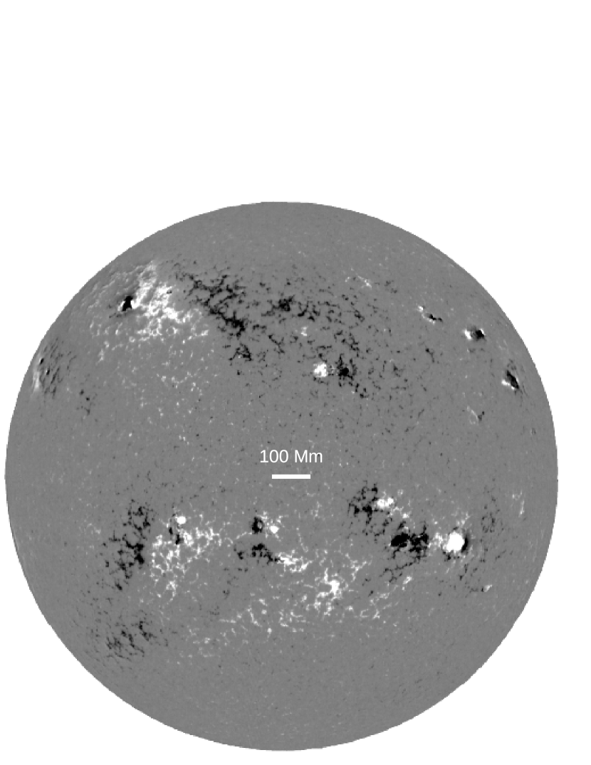
Figure 1.— Full disk solar magnetogram showing the line of sight magnetic field during a very active phase. Light (dark) shades correspond to positive (negative) values. Note the characteristic wavelength $\approx 100\,{\rm Mm}$ of regular sign changes.

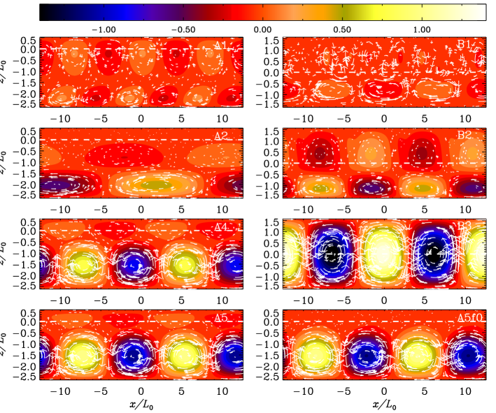
Figure 2.— Saturated magnetic background fields of the runs in Table 1. Colors and arrows indicate the vector potential $A_{y}$ and the magnetic field ${\bm{B}}$, respectively.

We define the $z$ dependent root-mean-squared Alfvén speed, $v_{\rm A}(z)$, and the quantity $\beta$, characterizing the subsurface concentration of $v_{\rm A}(z)$, as

$$v_{\rm A}(z)=\sqrt{\frac{\langle B^{2}\rangle_{x}(z)}{\mu_{0}\rho(z)}}\;,\quad\beta=\big{(}\max_{z\leq 0}\,{v_{\rm A}(z)}\big{)}/{c_{\rm sd}}.$$ (7)

In Fig. 3 we show the variation of $v_{\rm A}(z)/c_{\rm s}(z)$ with $z$ for all runs; more details are given in Table 1, where $z_{\rm m}$ is the position of the maximum in Eq. (7). We also show that the $f$-mode asymmetry, characterized by the quantity ${\cal A}_{\rm f}$ (defined below) increases with $z_{\rm m}$ and varies only weakly with $\beta$.

For a horizontally imposed uniform magnetic field, the $f$-mode frequency is well described by the dispersion relation (Chandrasekhar, 1961; Miles & Roberts, 1992; Miles et al., 1992)

$$\omega_{\rm fm}^{2}=c_{\rm fm}^{2}k_{x}^{2}+gk_{x}\frac{1-q}{1+q},$$ (8)

where $c_{\rm fm}^{2}=2{\rho_{\rm d}}v_{{\rm A}x\rm d}^{2}/({\rho_{\rm d}}+{\rho_{\rm u}})$ with $v_{{\rm A}x\rm d}$ being the Alfvén speed just below the interface; see Equation (21) of SBCR. Here, the second term on the right-hand side represents the (square of the) classical, unmagnetized $f$-mode frequency, to which the first term, being the magnetic contribution, always adds. Thus, horizontal magnetic fields lead to an increase in the $f$-mode frequency, but, as discussed by Murawski & Roberts (1993), turbulence without magnetic field leads to a decrease. SBCR found that also strong vertical magnetic fields lead to a decrease of the $f$-mode frequency for sufficiently large $\widetilde{k}_{x}$.

Berton & Heyvaerts (1987) analyzed the alterations of the $p$-mode frequencies in the presence of a nonuniform (piecewise uniform periodic) magnetic field, but they did not consider $f$-modes. It would be important to determine how a harmonic magnetic field affects the $f$-mode frequencies, but such calculations have not yet been done. Some qualitative insight can be gained from an analysis of the possible eigensolution spectra. In the linearized MHD equations, the coefficients of the perturbations $\bm{u}$, $\rho^{\prime}$, and $\bm{b}$, which are essentially determined by the background fields $\bm{U}_{0}$, $\rho_{0}$, and $\bm{B}_{0}$, are periodic in $x$ (or constant). Hence, the eigenmodes must in general comprise an infinitude of $x$ wavenumbers. With the spectra of the background fields derived above we expect for $\bm{u}$ and $\rho^{\prime}$ non-vanishing spectral amplitudes at $(\pm 2mN\pm l)k_{1}$, but for $\bm{b}$ at $\big{(}\pm(2m+1)N\pm l\big{)}k_{1}$, where $m=0,1,2,\ldots$, and $l$ is a fixed integer, $0\leq l\leq N/2$.

The described eigenmodes correspond to Bloch waves being bounded solutions of the stationary Schrödinger equation with a periodic potential. According to Bloch’s theorem they must have the form $c_{+}F(x)\exp{\rm i}k_{0}x+c_{-}F(-x)\exp(-{\rm i}k_{0}x)$, where $F(x)$ is a function with the same periodicity as the potential and $k_{0}$ is the so-called Bloch wavenumber (Berton & Heyvaerts, 1987). For our conditions, $k_{0}/k_{1}=l$ and can hence only adopt integers from 0 to $N/2$.

Table 1 Summary of simulations with $q=0.1$, $\nu/\eta=1$ and $\widetilde{k}_{\rm f}=20$. $\Delta{\omega}_{\rm f\pm}/{\omega}_{\rm f}$ are evaluated at $\widetilde{k}_{x}=9$.

Run	$\widetilde{k}^{B}_{x}$	$\widetilde{k}^{B}_{z}$	$\beta$	$\widetilde{z}_{\rm m}$	$\frac{\Delta{\omega}_{\rm f+}}{{\omega}_{\rm f}}$	$\frac{\Delta{\omega}_{\rm f-}}{{\omega}_{\rm f}}$	${\rm Re}$	${\rm Ma}$
A1	0.75	2.5	0.074	0	-	-	4.95	0.0198
A2	0.25	3.0	0.118	-1.5	0.33	0.23	9.67	0.0201
A4	0.50	2.0	0.234	-0.8	0.33	0.37	0.79	0.0032
A5	0.50	2.0	0.285	-0.8	0.44	0.41	1.15	0.0046
A5f0	0.50	2.0	0.278	-0.75	0.11	0.0	0.74	0.0030
B1	0.50	4.0	0.034	-0.3	-	-	0.05	0.0010
B2	0.50	2.0	0.104	-0.7	0.33	0.30	1.06	0.0042
B3	0.50	1.0	0.127	0	-	-	0.03	0.0006

3. Results

To demonstrate the effects of nonuniformity of the magnetic field, we study two types of cases: for the first one the domain is asymmetric with respect to the interface ($L_{z,\rm d}/L_{z,\rm u}=5$; Runs A1–A5), while symmetric for the second ($L_{z,\rm d}=L_{z,\rm u}$; Runs B1–B3).

Figure 3.— Vertical profiles of the ratio of Alfvén to sound speed, $v_{\rm A}/c_{\rm s}$ in upper two panels; dash-dotted line: position of the interface. ${\cal A}_{\rm f}$ as a function of $z_{\rm m}$ in panel (c) showing the fit ${\cal A}_{\rm f}=a_{0}+a_{1}z_{\rm m}$ with $a_{0}=0.42$ and $a_{1}=0.67$ for all values of $\beta$ (solid line); ${\cal A}_{\rm f}$ normalized by this fit as a function of $\beta$ in panel (d).

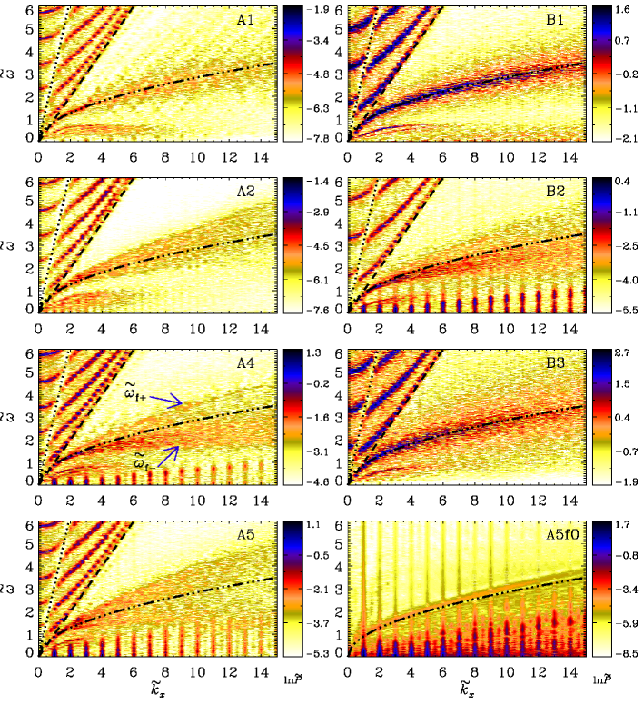
Figure 4.— $k\omega$ diagrams corresponding to the runs of Table 1; $L_{z\rm d}/L_{z\rm u}=5$ for models A1–5 and $L_{z\rm d}=L_{z\rm u}$ for models B1–3. The dotted and dashed lines show $\omega=c_{\rm su}k_{x}$ and $\omega=c_{\rm sd}k_{x}$, respectively; dash-dotted curves show $\omega_{\rm f}$ (the classical $f$-mode). In panel A4, the arrows indicate the estimated edges of the $f$-mode fan at $\widetilde{k}_{x}=9$.

The corresponding $k\omega$ diagrams are shown in Fig. 4. Similar to the nonmagnetic or weakly magnetized cases studied by SBCR, we see $p$-modes above the line $\omega=c_{\rm sd}k_{x}$ with an apparent discontinuity at $\omega=c_{\rm su}k_{x}$, and indications of $g$-modes at $\widetilde{k}_{x}<4$ and $\widetilde{\omega}=0.5$–$0.8$. However, the $f$-mode now fans out and spans a trumpet-shaped structure around the non-magnetic $f$-mode frequency $\sqrt{gk}$. The more the magnetic field is pushed toward the bottom of the domain, the more asymmetric this expansion appears to be with respect to the usual $f$-mode in the unmagnetized case.

To quantify the fanning out of the $f$-mode, we denote the upper and lower edges of the fan at a given value of ${k}_{x}$ by ${\omega}_{\rm f+}$ and ${\omega}_{\rm f-}$, respectively. In general, the fan is asymmetric with respect to the classical $f$-mode ($\omega_{\rm f}$). Let us represent this asymmetry at any given ${k}_{x}$ by ${\cal A}_{\rm f}=\Delta{\omega}_{\rm f+}/\Delta{\omega}_{\rm f-}$, where $\Delta{\omega}_{\rm f\pm}=|\omega_{\rm f\pm}-\omega_{\rm f}|$ are the frequency spreads above and below $\omega_{\rm f}$; see Table 1 for $\Delta{\omega}_{\rm f\pm}/\omega_{\rm f}$ at $\widetilde{k}_{x}=9$. We find that at $\widetilde{k}_{x}=15$, the total relative spread, $(\Delta{\omega}_{\rm f+}+\Delta{\omega}_{\rm f-})/\omega_{\rm f}$, can be as large as $1.1$, which further increases with increasing $\beta$ for fixed $z_{\rm m}$; see Runs A4 and A5 in Fig. 4. Note that ${\cal A}_{\rm f}$ can take values both larger and smaller than unity, as may be seen by comparing Run A2 with Runs A4 or A5 in Fig. 4; see also Table 1 and Fig. 3.

In addition, we see as a qualitatively new feature a regular pattern of vertical stripes at multiples of $2\widetilde{k}_{x}^{B}$ all the way up to $\widetilde{k}_{x}=14$, which appears unconnected with the $f$-mode. (In the spectra of $\bm{B}$ the stripes appear at odd multiples of $\widetilde{k}_{x}^{B}$.) They are absent if $\bm{B}_{0}$ is independent of $z$ (${k}^{B}_{z}=0$; not shown), but most pronounced when the magnetic field is concentrated in the lower part of the domain. These are also cases in which the $f$-mode appears most fanned out. The stripes appear weaker when the magnetic field is symmetric about the interface at $z=0$ (Run B3) or when it is generally weak (Runs A1, A2, and B1). Given that they are persistent after switching off the random hydrodynamic forcing (see Run A5f0 in Fig. 4), they can be identified to indicate at least one unstable eigensolution. Note that for a fixed $\omega$ an infinitude of $k_{x}$ belongs to the same eigenmode. The discrete $\omega$ spots within each stripe may either belong to different unstable eigenmodes or represent overtones of a single mode. The velocity field of the stripes is close to solenoidal and their occurrence and amplitude are strongly dependent on the strength of $\bm{B}_{0}$. So we propose to consider them as shear Alfvén modes having become unstable due to the inhomogeneity of $\bm{B}_{0}$. A similar transition is observed in whistler waves which become unstable for suitably non-uniform background fields (Rheinhardt & Geppert, 2002).

Remarkably, the unstable mode(s) excite $f$ modes, but without fanning them out, whereas $p$ modes remain unexcited (Panel A5f0). Comparing panels A5 and A5f0 suggests that the fanning out requires not just a non-uniform magnetic field, but also the presence of random forcing. However, the fact that A5f0 exhibits only a single line and no fan might indicate a physical difference between the fan and the regular $f$-mode. We also note that the expansion of the $f$-mode can still be seen when the vertical stripes are weak or absent (especially in Run A2), but in Run B1, where the field is less deep and the domain symmetric about $z=0$, the $f$-mode lacks a clear trumpet shape.

4. Conclusions

The present study was aimed at identifying diagnostic signatures of spatial variability of the magnetic field. Indeed, we find in the fanning out of the $f$-mode and in a pattern of vertical stripes in the $k\omega$ diagram such characteristic features which have not been reported in earlier helioseismic studies.

The fanning out of the $f$-mode is different from the case of capillary waves, where instead a “bifurcation” of the $f$-mode in deep water waves is caused by surface tension (Dias & Kharif, 1999). In the present case, the width of the fan and its asymmetry appear to characterize the magnetic field strength. Independent from that, the horizontal variability of the underlying magnetic field is reflected in the presence of vertical stripes in the diagnostic $k\omega$ diagram at even multiples of the horizontal wavenumber of the magnetic field. We have proven that the stripes can be assigned to one or perhaps several unstable eigenmodes, most likely of shear Alfvén type.

The spatial variation of the photospheric field seen in Fig. 1 with a wavelength of about $100\,{\rm Mm}$ corresponds to a wavenumber $k_{x}=0.06\,{\rm Mm}^{-1}$, so the spherical harmonic degree would be $\ell\approx k_{x}R\approx 40$, where $R=700\,{\rm Mm}$ is the solar radius. On the other hand, as discussed in SBCR, the pressure scale height $H_{\rm d}$ is the only intrinsic length scale in the underlying nonmagnetic problem, and so the range of dimensionless wavenumbers resolved in our simulations is $k_{x}\gamma H_{\rm d}\approx 2$–$15$. With $\gamma H_{\rm d}\approx 0.5\,{\rm Mm}$, this corresponds to values of $\ell$ that are much larger than those of the pattern seen in Fig. 1. The question is thus, whether in the simulations a magnetic field with a much larger horizontal wavelength would still be able to produce signatures that could be discerned from the diagnostic $k\omega$ diagram. This is not obvious, given that values of $k_{x}=0.06\,{\rm Mm}^{-1}$ correspond to $k_{x}\gamma H_{\rm d}=0.03$, where with our box geometry we are unable to produce clear features. Thus, while it is impossible to make a clear case for helioseismic applications, our work has opened the possibility for more targeted searches both theoretically and observationally.

References

- Berton & Heyvaerts (1987) Berton, R., & Heyvaerts, J. 1987, Solar Phys., 109, 201
- Brandenburg (2005) Brandenburg, A. 2005, ApJ, 625, 539
- Brandenburg et al. (2014) Brandenburg, A., Gressel, O., Jabbari, S., Kleeorin, N., & Rogachevskii, I. 2014, A&A, 562, A53
- Caligari et al. (1995) Caligari, P., Moreno-Insertis, F., & Schüssler, M. 1995, ApJ, 441, 886
- Chandrasekhar (1961) Chandrasekhar, S. 1961, Hydrodynamic and Hydromagnetic Stability (Dover Publications, New York)
- Daiffallah et al. (2011) Daiffallah, K., Abdelatif, T., Bendib, A., Cameron, R., & Gizon, L. 2011, Solar Phys., 268, 309
- Dias & Kharif (1999) Dias, F., & Kharif, C. 1999, Ann. Rev. Fluid Mech., 31, 301
- Felipe et al. (2012) Felipe, T., Braun, D., Crouch, A., & Birch, A. 2012, ApJ, 757, 148
- Felipe et al. (2013) Felipe, T., Crouch, A., & Birch, A. 2013, ApJ, 775, 74
- Gizon et al. (2010) Gizon, L., Birch, A. C., & Spruit, H. C. 2010, ARA&A, 48, 289
- Hanasoge et al. (2008) Hanasoge, S. M., Birch, A. C., Bogdan, T. J., & Gizon, L. 2008, ApJ, 680, 774
- Ilonidis et al. (2011) Ilonidis, S., Zhao, J., & Kosovichev, A. 2011, Science, 333, 993
- Kitchatinov & Mazur (2000) Kitchatinov, L. L., & Mazur, M. V. 2000, Solar Phys., 191, 325
- Kleeorin et al. (1996) Kleeorin, N., Mond, M., & Rogachevskii, I. 1996, A&A, 307, 293
- Miles & Roberts (1989) Miles, A. J., & Roberts, B. 1989, Solar Phys., 119, 257
- Miles & Roberts (1992) Miles, A. J., & Roberts, B. 1992, Solar Phys., 141, 205
- Miles et al. (1992) Miles, A. J., Allen, H. R., & Roberts, B. 1992, Solar Phys., 141, 235
- Murawski & Roberts (1993) Murawski, K. and Roberts, B. 1993, A&A, 272, 595
- Parker (1975) Parker, E. N. 1975, ApJ, 198, 205
- Rae & Roberts (1981) Rae, I. C., & Roberts, B. 1981, Geophys. Astrophys. Fluid Dyn., 18, 197
- Rheinhardt & Geppert (2002) Rheinhardt, M., & Geppert, U. 2002, Phys. Rev. Lett., 88, 101103
- Roberts (1981) Roberts, B. 1981, Solar Phys., 69, 27
- Singh et al. (2014) Singh, N. K., Brandenburg, A., Chitre, S. M., & Rheinhardt, M. 2014, MNRAS, submitted (SBCR)
- Tao et al. (1998) Tao, L., Weiss, N. O., Brownjohn, D. P., & Proctor, M. R. E. 1998, ApJ, 496, L39