Abstract

We derive the exact S-matrix for the scattering of particular representations of the centrally-extended $\mathfrak{psu}(1|1)^{2}$ Lie superalgebra, conjectured to be related to the massive modes of the light-cone gauge string theory on $AdS_{2}\times S^{2}\times T^{6}$. The S-matrix consists of two copies of a centrally-extended $\mathfrak{psu}(1|1)$ invariant S-matrix and is in agreement with the tree-level result following from perturbation theory. Although the overall factor is left unfixed, the constraints following from crossing symmetry and unitarity are given. The scattering involves long representations of the symmetry algebra, and the relevant representation theory is studied in detail. We also discuss Yangian symmetry and find it has a standard form for a particular limit of the aforementioned representations. This has a natural interpretation as the massless limit, and we investigate the corresponding limits of the massive S-matrix. Under the assumption that the massless modes of the light-cone gauge string theory transform in these limiting representations, the resulting S-matrices would provide the building blocks for the full S-matrix. Finally, some brief comments are given on the Bethe ansatz.

1 Introduction

The remarkable successes of integrability techniques in the study of the $AdS_{5}\times S^{5}$ superstring [2, 3] motivates the application of these methods to other integrable string backgrounds with less supersymmetry [4]. In this work we investigate the $AdS_{2}\times S^{2}\times T^{6}$ background supported by Ramond-Ramond fluxes in Type II superstring theory, which preserves a quarter of the supersymmetries. These can be found as the near-horizon limit of various intersecting brane solutions of Type IIB supergravity, which are related by T-duality [5]. The dual [6] should be a one-dimensional CFT, and is understood to either be a superconformal quantum-mechanical system or a chiral two-dimensional CFT [7].

The $AdS_{2}\times S^{2}$ part of the background can be written as a Metsaev-Tseytlin [8] type supercoset model [9] for $PSU(1,1|2)/SO(1,1)\times SO(2)$. The algebra $\mathfrak{psu}(1,1|2)$ has a $\mathbb{Z}_{4}$ automorphism and hence the supercoset model is classically integrable via the same construction as for the $AdS_{5}\times S^{5}$ case [10]. While there exists a classical truncation of the Green-Schwarz action [11] for the $AdS_{2}\times S^{2}\times T^{6}$ geometry to the supercoset degrees of freedom, there is no $\kappa$-symmetry gauge choice which decouples them from the remaining fermions [12]. The integrability of the Green-Schwarz action for the complete background has been demonstrated to quadratic order in fermions [12, 13].

The aim of this paper is to use symmetries and integrability to construct exact S-matrices for the scattering of the worldsheet excitations of the decompactified light-cone gauge [14] $AdS_{2}\times S^{2}\times T^{6}$ superstring. These S-matrices describe the scattering above the BMN vacuum [15], a point-like string moving at the speed of light on a great circle of the two-sphere. The light-cone gauge-fixed Lagrangian [16, 17] is in general rather complicated with the interaction terms breaking two-dimensional Lorentz invariance. The quadratic action is however Lorentz invariant and describes $2+2$ (bosons+fermions) massive modes, the bosons of which are associated to the transverse directions in $AdS_{2}\times S^{2}$, and $6+6$ massless modes, associated to the $T^{6}$.

In the $AdS_{5}\times S^{5}$ light-cone gauge-fixed theory all of the excitations have equal non-vanishing mass and furthermore the symmetries completely fix the S-matrix up to an overall phase [18, 19, 20]. Here the situation is more similar to $AdS_{3}\times S^{3}\times T^{4}$ for which there are $4+4$ massive and $4+4$ massless excitations. In this case the symmetries of the supercoset leaving the BMN string invariant can be used to conjecture an exact S-matrix for the scattering of the massive modes [21, 22] (see also the review [23]). Following a similar approach we observe that the subalgebra of the $\mathfrak{psu}(1,1|2)$ symmetry of the $AdS_{2}\times S^{2}$ supercoset preserved by the BMN string is given by $\mathfrak{psu}(1|1)^{2}\ltimes\mathbb{R}$. Relaxing the level-matching condition we extend this algebra by two additional central extensions and conjecture the exact S-matrix for the scattering of massive modes up to an overall factor.

The resulting massive S-matrix satisfies crossing symmetry [24] and is unitarity so long as the overall factor satisfies the relevant identities. Here the setup is more similar to the $AdS_{5}\times S^{5}$ case as opposed to the $AdS_{3}\times S^{3}\times T^{4}$ case for which there were multiple phases related by crossing transformations [25]. It was observed in [17] that the one-loop logarithms in the massive S-matrix for $AdS_{2}\times S^{2}\times T^{6}$ are consistent with the one-loop phase being related to the Hernandez-Lopez phase [26, 27]. Finally, the near-BMN expansion of the exact result is consistent with perturbative computations [16, 17, 28].

While many features of the construction are similar to the $AdS_{5}\times S^{5}$ and $AdS_{3}\times S^{3}\times T^{4}$ cases, there are some important differences. In particular, unlike for the $AdS_{5}\times S^{5}$ and $AdS_{3}\times S^{3}\times T^{4}$ superstrings, the representations we are scattering turn out to be long and hence there is no shortening condition to be interpreted as the dispersion relation. An additional consequence is that the symmetries do not completely fix the S-matrix up to a single overall factor, rather there is an additional undetermined function that can be found by demanding the Yang-Baxter equation is satisfied. These properties are reminiscent of similar features seen for the scattering of long representations of $\mathfrak{psu}(2|2)\ltimes\mathbb{R}^{3}$ [29] and also in the Pohlmeyer reduction of strings on $AdS_{2}\times S^{2}$ [30].

The S-matrix has an accidental $U(1)$ symmetry under which the fermions are charged, while the bosons are not. From the perspective of the complete $AdS_{2}\times S^{2}\times T^{6}$ superstring this $U(1)$ originates from the $T^{6}$ compact space [17]. Furthermore, its presence appears to be important to have any hope of applying a Bethe ansatz construction as it allows one to define a pseudovacuum. A conjecture for a set of asymptotic Bethe ansatz equations was given in [12], however, due to the somewhat involved structure of the S-matrix it is not clear how to derive them.

It is not currently known how the massless modes transform under the symmetry group of the light-cone gauge-fixed theory, and therefore it is not possible to completely determine the corresponding S-matrices. Furthermore, they may depend on the choice of Type II background [5] – in the decompactified light-cone gauge-fixed theory the $T^{6}$ formally has an $SO(6)$ symmetry, however, this will be broken by the presence of Ramond-Ramond fluxes. Initial investigations in this direction for a particular Type IIA background were carried out in [16, 17], in which case the $SO(6)$ is broken to $U(3)$. However, different backgrounds related by T-duality will naively lead to different subgroups [5].

Here we take an alternative (partial) approach to the question of massless modes motivated by the recent explicit computation of the light-cone gauge symmetry algebra for the $AdS_{3}\times S^{3}\times T^{4}$ superstring [31], the $AdS_{5}\times S^{5}$ version of which was constructed in [32]. Under the assumption that a similar outcome occurs for the $AdS_{2}\times S^{2}\times T^{6}$ superstring one may expect the massless modes to transform in representations of $\mathfrak{psu}(1|1)^{2}\ltimes\mathbb{R}^{3}$. We further rely on the fact that the two-dimensional modules we work with are rather general in their parametrization, and assume that the massless representations take the same form as the massive ones, provided one sends the mass parameter $m$ to zero. Upon adopting these assumptions, the S-matrices describing their scattering should be built from the massless limits (one massless and one massive or two massless particles) of the massive S-matrix. How these building blocks are precisely put together and the corresponding overall number of undetermined phases (of which there may be many) will depend on the complete symmetry of the light-cone gauge-fixed backgrounds (including the subgroup of $SO(6)$ preserved by the fluxes), an analysis that we leave for future work.

The structure of the paper is as follows. In section 2 we describe the near-BMN symmetry algebra and investigate its representation theory. This symmetry is then used in section 3 to determine the exact S-matrix up to an overall phase. We determine the constraints that the phase should satisfy for crossing symmetry and unitarity and compare with perturbation theory. In section 4 we discuss when this symmetry can be extended to a Yangian, finding that it can be done in the standard form for the massless case. Using this Yangian symmetry in section 5 we then construct the massless version of the S-matrix and briefly explore the notions of crossing symmetry and unitarity in this limit. In section 6 we give some initial considerations of the algebraic Bethe ansatz, noting in particular the existence of a pseudovacuum, and we conclude in section 7 with some comments.

2 Symmetry for massive modes of $\mathbf{AdS_{2}\times S^{2}}$

The BMN light-cone gauge $AdS_{2}\times S^{2}\times T^{6}$ superstring action describes $2+2$ massive and $6+6$ massless modes. The algebra underlying the scattering of the massive modes is expected to be $\mathfrak{psu}(1|1)^{2}\ltimes\mathbb{R}^{3}$, which is found by considering the subalgebra of $\mathfrak{psu}(1,1|2)$ that is preserved by the BMN geodesic. We expect two additional central extensions to appear, by analogy with the $AdS_{5}\times S^{5}$ case, in the decompactification limit and relaxing the level-matching condition.

Although a full off-shell analysis, as in [32, 31], would be necessary (and is planned for future work) to confirm the nature of the central extensions, in this paper we construct the massive S-matrix on the basis of certain assumptions. The first assumption is the analogy with higher dimensional AdS/CFT integrable systems, and in particular the way the central extensions manifest themselves. This assumption is also motivated by perturbation theory, in particular the symmetry algebra being given by two copies of a centrally-extended algebra with the centres identified, seems to be suggested, for instance, by the work of [17]. The second crucial assumption is integrability itself. On the one hand, integrability should work to complete the perturbative results into the structure of classified representations of superalgebras. On the other hand, it should maintain the tree-level factorized form of the S-matrix at higher string loops.

With these assumptions in mind, we will nevertheless pursue a broad approach and explore the most general central extension based on the available kinematical algebra. We denote the massive boson associated to the transverse direction of $S^{2}$ as $y$ and the corresponding boson for $AdS_{2}$ as $z$. The two massive fermions will be represented as two real Grassmann fields $\zeta$ and $\chi$. We can then formally define the following tensor product states

$$\begin{split}\left|y\right>=\left|\phi\right>\otimes\left|\phi\right>\ ,\qquad&\left|z\right>=\left|\psi\right>\otimes\left|\psi\right>\ ,\\ \left|\zeta\right>=\left|\phi\right>\otimes\left|\psi\right>\ ,\qquad&\left|\chi\right>=\left|\psi\right>\otimes\left|\phi\right>\ ,\end{split}$$ (2.1)

where $\phi$ is bosonic and $\psi$ is fermionic, such that we expect one of the factors of $\mathfrak{psu}(1|1)$ to act on each of the two entries. Furthermore, as a consequence of the form of the symmetry algebra and the integrability of the theory [12, 16] we expect that the S-matrix for $y$, $z$, $\zeta$ and $\chi$ can be constructed as a graded tensor product of an S-matrix for $\phi$ and $\psi$, with each factor S-matrix invariant under the symmetry $\mathfrak{psu}(1|1)\ltimes\mathbb{R}^{3}$.

In this section we will construct the relevant massive representation of $\mathfrak{psu}(1|1)\ltimes\mathbb{R}^{3}$. This representation has an obvious massless limit, and, by analogy with the construction for $AdS_{3}\times S^{3}\times T^{4}$ [31], one may expect the massless modes to also transform in representations of $\mathfrak{psu}(1|1)\ltimes\mathbb{R}^{3}$ in the light-cone gauge-fixed theory. The massless limit is discussed in detail in section 5.

Let us also briefly mention that there is an additional $U(1)$ outer automorphism symmetry [17] of the S-matrix (3), under which the $\mathfrak{psu}(1|1)$ factors transform in the vector representation. The origin of this $U(1)$ symmetry is the $T^{6}$ compact space that is required for a consistent 10-d superstring theory. Under this symmetry $(\zeta,\chi)^{T}$ also transforms as a vector, while the bosons are uncharged. It is worth noting that taking the tensor product of two copies of any S-matrix for $\phi$ and $\psi$ preserving the value of $(-1)^{F}$, where $F$ is the fermion number operator, we find that the $U(1)$ symmetry is present so long as a certain quadratic relation between the parametrizing functions is satisfied (see appendix Appendix A: Expansion of tensor product and $\mathbf{U(1)}$ symmetry). In the case of interest, this quadratic identity turns out to be true just from demanding invariance under the $\mathfrak{psu}(1|1)\ltimes\mathbb{R}^{3}$ symmetry and satisfaction of the Yang-Baxter equation. The $U(1)$ does not act in a well-defined way on the individual factor S-matrices and hence for now we will ignore it. We will reconsider it in section 6, where it will play a role in defining a pseudovacuum, an important first step in the algebraic Bethe ansatz.

2.1 The $\mathfrak{gl}(1|1)$ Lie superalgebra and its representations

Let us start by summarizing the relevant information from [33] regarding the Lie superalgebra $\mathfrak{gl}(1|1)$ and its representations. There are two bosonic generators $\mathfrak{N}$ and $\mathfrak{C}$, with $\mathfrak{C}$ central, and two fermionic generators $\mathfrak{Q}$ and $\mathfrak{S}$. The commutation relations read

$$[\mathfrak{N},\,\mathfrak{Q}]=-\mathfrak{Q}\ ,\qquad[\mathfrak{N},\,\mathfrak{S}]=\mathfrak{S}\ ,\qquad\{\mathfrak{Q},\,\mathfrak{S}\}=2\mathfrak{C}\ .$$ (2.2)

The typical (long) irreps are the 2-dimensional Kac modules $\langle C,\nu\rangle$, defined by the following non-zero entries on a boson-fermion $(|\phi\rangle,\,|\psi\rangle)$ pair of states:

$$\mathfrak{Q}\left|\phi\right>=\left|\psi\right>\ ,\qquad\mathfrak{S}\left|\psi\right>=2\,C\left|\phi\right>\ ,\qquad\mathfrak{N}\left|\phi\right>=\nu\left|\phi\right>\ ,\qquad\mathfrak{N}\left|\psi\right>=(\nu-1)\left|\psi\right>\ ,$$

$$\mathfrak{C}\left|\Phi\right>=C\left|\Phi\right>\ \qquad\forall\,\,\,|\Phi\rangle\,\in\,\{|\phi\rangle,\,|\psi\rangle\},\qquad C,\nu\,\in\,\mathbb{C},\qquad C\neq 0.$$ (2.3)

We have summarized the generator action in figure 1.

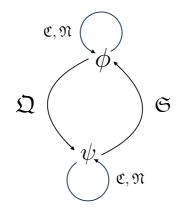
Figure 1: The Kac module $\langle C,\nu\rangle$.

As long as $C\neq 0$, this module is isomorphic to the anti-Kac module $\overline{\langle C,\nu\rangle}$

$$\mathfrak{Q}\left|\psi\right>=2\,C\left|\phi\right>\ ,\qquad\mathfrak{S}\left|\phi\right>=\left|\psi\right>\ ,\qquad\mathfrak{N}\left|\phi\right>=(\nu-1)\left|\phi\right>\ ,\qquad\mathfrak{N}\left|\psi\right>=\nu\left|\psi\right>\ ,$$

$$\mathfrak{C}\left|\Phi\right>=C\left|\Phi\right>\ \qquad\forall\,\,\,|\Phi\rangle\,\in\,\{|\phi\rangle,\,|\psi\rangle\},\qquad C,\nu\,\in\,\mathbb{C},\qquad C\neq 0.$$ (2.4)

However, if $C=0$, the two modules are not isomorphic and they are no longer irreducible. Rather they become reducible but indecomposable.

To elucidate further we introduce the 1-dimensional modules $\langle\mu\rangle$, which form the atypical (short) irreps of $\mathfrak{gl}(1|1)$. These irreps are characterized by the vanishing of all generators except $\mathfrak{N}$, which acts with eigenvalue $\mu$. We then see that for the Kac module, $\langle 0,\nu\rangle$, the fermion $|\psi\rangle$ spans a sub-representation $\langle\nu-1\rangle$, and the indecomposable is denoted as

$$\langle\nu-1\rangle\,\longleftarrow\langle\nu\rangle\ .$$ (2.5)

The anti-Kac module $\overline{\langle 0,\nu\rangle}$ is also reducible but indecomposable and is denoted as

$$\langle\nu-1\rangle\,\longrightarrow\langle\nu\rangle\ ,$$ (2.6)

with the fermion $|\psi\rangle$ once again spanning the sub-representation $\langle\nu\rangle$. This indecomposable is not isomorphic to $\langle 0,\nu\rangle$. Let us mention that modding out the indecomposable representations by their sub-representations one obtains the factor representations, which in this case are isomorphic to the short 1-dimensional $\langle\mu\rangle$ modules and are spanned by the boson $|\phi\rangle$.

If we take the tensor product of two typical modules, we get

$$\langle C_{1},\nu_{1}\rangle\otimes\langle C_{2},\nu_{2}\rangle\,=\,\langle C_{1}+C_{2},\nu_{1}+\nu_{2}-1\rangle\oplus\langle C_{1}+C_{2},\nu_{1}+\nu_{2}\rangle\qquad\mbox{if}\,\,\,C_{1}+C_{2}\neq 0\ ,$$

$$\langle C_{1},\nu_{1}\rangle\otimes\langle-C_{1},\nu_{2}\rangle\,=\,P_{\nu_{1}+\nu_{2}}\ ,$$ (2.7)

where $P_{\nu}$ is the so-called projective module

$$\langle\nu\rangle\,\longrightarrow\,\langle\nu+1\rangle\oplus\langle\nu-1\rangle\,\longrightarrow\,\langle\nu\rangle\ ,$$ (2.8)

on which $\mathfrak{C}$ acts identically as zero. The rightmost 1-dimensional short sub-module $\langle\nu\rangle$ is known as the socle of $P_{\nu}$.

Since $\mathfrak{N}$ does not appear on the r.h.s. of the commutation relations, the algebra $\mathfrak{gl}(1|1)$ has a non-trivial ideal generated by $\mathfrak{Q}$, $\mathfrak{S}$ and $\mathfrak{C}$. This ideal is the superalgebra $\mathfrak{sl}(1|1)$. Furthermore, this algebra is also not simple, as $\mathfrak{C}$, being central, is a non-trivial ideal. Additionally modding out $\mathfrak{C}$ gives the algebra $\mathfrak{psl}(1|1)$, which is still not simple, as the two remaining anti-commuting fermionic generators each form a separate ideal. The fact that $\mathfrak{psl}(1|1)$ is not simple sets this algebra outside the classification of the possible central extensions of basic classical Lie superalgebras presented in [34].

2.2 The centrally-extended $\mathfrak{psu}(1|1)$ Lie superalgebra

We are now ready to introduce the centrally-extended version of the algebra we discussed above, which, as anticipated by the discussion at the beginning of section 2, we conjecture to be relevant for the scattering of the massive modes of the $AdS_{2}\times S^{2}\times T^{6}$ superstring. The algebra $\mathfrak{psu}(1|1)\ltimes\mathbb{R}^{3}$ is defined by the commutation relations

$$\{\mathfrak{Q},\,\mathfrak{Q}\}=2\mathfrak{P}\ ,\qquad\{\mathfrak{S},\,\mathfrak{S}\}=2\mathfrak{K}\ ,\qquad\{\mathfrak{Q},\,\mathfrak{S}\}=2\mathfrak{C}\ .$$ (2.9)

The states $|\phi\rangle$ and $|\psi\rangle$, introduced in (2.1), then transform in the following representation:

$$\mathfrak{Q}\left|\phi\right>=a\left|\psi\right>\ , \mathfrak{Q}\left|\psi\right>=b\left|\phi\right>\ , \mathfrak{S}\left|\phi\right>=c\left|\psi\right>\ , \mathfrak{S}\left|\psi\right>=d\left|\phi\right>\ ,$$

$$\mathfrak{C}\left|\Phi\right>=C\left|\Phi\right>\ , \mathfrak{P}\left|\Phi\right>=P\left|\Phi\right>\ , \mathfrak{K}\left|\Phi\right>=K\left|\Phi\right>\ .$$ (2.10)

Here $a$, $b$, $c$, $d$, $C$, $P$ and $K$ are the representation parameters that will eventually be functions of the energy and momentum of the states. For the supersymmetry algebra to close the following conditions should be satisfied

$$\begin{split}ab=P\ ,\qquad cd=K\ ,\qquad&ad+bc=2C\ .\end{split}$$ (2.11)

This representation corresponds to the typical (long) Kac module $\langle C,\nu\rangle$ discussed in the previous section. We have summarized the generator action in figure 2.

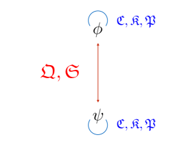
Figure 2: The 2-dimensional module of the centrally-extended algebra (several lines are superimposed).

We will be interested in a particular real form of the algebra (2.9), which is given by

$$\mathfrak{Q}^{\dagger}=\mathfrak{S}\ ,\qquad\mathfrak{P}^{\dagger}=\mathfrak{K}\ ,\qquad\mathfrak{C}^{\dagger}=\mathfrak{C}\ .$$ (2.12)

These relations further constrain the representation parameters as follows

$$a^{*}=d\ ,\qquad b^{*}=c\ ,\qquad C^{*}=C\ ,\qquad P^{*}=K\ .$$ (2.13)

The closure conditions (2.11) imply that

$$C^{2}=\frac{(ad-bc)^{2}}{4}+PK\ .$$ (2.14)

Unlike the $AdS_{5}\times S^{5}$ case, with the larger symmetry algebra $\mathfrak{psu}(2|2)^{2}\ltimes\mathbb{R}^{3}$, here we are scattering long representations and hence there is no shortening condition – that is, $ad-bc$ is free to take any value, which we denote

$$m\equiv ad-bc\ .$$ (2.15)

The reality conditions (2.13) imply that $m$ is real. From (2.14) we then have

$$(C+\frac{m}{2})(C-\frac{m}{2})=PK>0\ ,$$ (2.16)

also as a consequence of the reality conditions (2.13). Motivated by the fact that $C$ will later be associated to an energy, we will take it to be positive. However, let us point out that the algebraic analysis we perform in this paper is largely insensitive to this choice, and hence it does not represent a loss of generality. If we make this positivity assumption, it immediately follows that both $(C+\frac{m}{2})$ and $(C-\frac{m}{2})$ are also positive. The analogy with the higher dimensional AdS/CFT cases suggests that we should associate (the absolute value of) $m$ with the mass of the scattering particle. Later it will be useful to solve the set of equations (2.11) for $a$, $b$, $c$ and $d$ in terms of $m$, $C$, $P$ and $K$

$$a=\, \alpha\,e^{-\frac{i\pi}{4}}\big{(}C+\frac{m}{2}\big{)}^{\frac{1}{2}}\ , \ b=\, \alpha^{-1}e^{\frac{i\pi}{4}}\big{(}C+\frac{m}{2}\big{)}^{-\frac{1}{2}}P\ ,$$

$$c=\, \alpha\,e^{-\frac{i\pi}{4}}\big{(}C+\frac{m}{2}\big{)}^{-\frac{1}{2}}K\ , d=\, \alpha^{-1}e^{\frac{i\pi}{4}}\big{(}C+\frac{m}{2}\big{)}^{\frac{1}{2}}\ .$$ (2.17)

Here $\alpha$ is a phase parametrizing the normalization of the fermionic states with respect to the bosonic states and can be a function of the central extensions.

To define the action of this symmetry on the two-particle states we need to introduce the coproduct

$$\Delta(\mathfrak{Q}) =\mathfrak{Q}\otimes\mathbf{1}+\mathfrak{U}\otimes\mathfrak{Q}\ , \Delta(\mathfrak{S}) =\mathfrak{S}\otimes\mathbf{1}+\mathfrak{U}^{-1}\otimes\mathfrak{S}\ ,$$

$$\Delta(\mathfrak{P}) =\mathfrak{P}\otimes\mathbf{1}+\mathfrak{U}^{2}\otimes\mathfrak{P}\ , \Delta(\mathfrak{C}) =\mathfrak{C}\otimes\mathbf{1}+\mathbf{1}\otimes\mathfrak{C}\ , \Delta(\mathfrak{K}) =\mathfrak{K}\otimes\mathbf{1}+\mathfrak{U}^{-2}\otimes\mathfrak{K}\ ,$$ (2.18)

and the opposite coproduct, defined as

$$\Delta^{\text{op}}(\mathfrak{J})=\mathcal{P}\,\Delta(\mathfrak{J})\ ,$$ (2.19)

where $\mathfrak{J}$ is an arbitrary abstract generator (prior to considering a representation), and $\mathcal{P}$ defines the graded permutation of the tensor product.

The coproduct differs from the trivial one by the introduction of a new abelian generator $\mathfrak{U}$, with $\Delta(\mathfrak{U})=\mathfrak{U}\otimes\mathfrak{U}$ [35]. This is done according to a $\mathbb{Z}$-grading of the algebra, whereby the charges $-2,-1,1$ and $2$ are associated to the generators $\mathfrak{K}$, $\mathfrak{S}$, $\mathfrak{Q}$ and $\mathfrak{P}$ respectively, while $\mathfrak{C}$ remains uncharged. The action of $\mathfrak{U}$ on the single-particle states is given by

$$\mathfrak{U}\left|\phi\right>=U\left|\phi\right>\ ,\qquad\qquad\mathfrak{U}\left|\psi\right>=U\left|\psi\right>\ .$$ (2.20)

This braiding allows for the existence of a non-trivial S-matrix.

One important consequence of the non-trivial braiding (2.18) is that it leads to a constraint between $U$ and the eigenvalues of the central charges. This follows from the requirement that, to admit an S-matrix, the coproduct of any central element should be equal to its opposite. This implies

$$\mathfrak{P}\propto(1-\mathfrak{U}^{2})\ ,\qquad\qquad\mathfrak{K}\propto(1-\mathfrak{U}^{-2})\ .$$ (2.21)

We fix the normalization of $\mathfrak{P}$ relative to $\mathfrak{K}$ by taking both constants of proportionality to be equal to $\tfrac{1}{2}{\rm h}$ where the reality conditions (2.13) require that ${\rm h}$ is real. The parameter ${\rm h}$ is a coupling constant and eventually should be fixed in terms of the string tension, which we will return to in section 3.2. Acting on the single-particle states then gives us the relations

$$P=\frac{{\rm h}}{2}\,(1-U^{2})\ ,\qquad\qquad K=\frac{{\rm h}}{2}\,(1-U^{-2})\ ,$$ (2.22)

where $U$ should satisfy, as a consequence of (2.13), the following reality condition

$$U^{*}=U^{-1}\ .$$ (2.23)

The relation (2.14) in terms of $C$, $U$ and $m$ is then given by

$$C^{2}=\frac{m^{2}-{\rm h}^{2}(U-U^{-1})^{2}}{4}\ .$$ (2.24)

While this is a single equation for three undetermined parameters, we will later still attempt to interpret it as a dispersion relation with $C$, $U$ and $m$ defined in terms of just two kinematic variables, the energy and momentum. These precise definitions are not fixed by symmetry considerations, and hence should be found from direct string computations.

It is now useful to introduce the Zhukovsky variables $x^{\pm}$, in terms of which we will write the S-matrix, in place of the central extensions, $C$ and $U$. These are defined as [18, 36]

$$U^{2}=\frac{x^{+}}{x^{-}}\ ,\qquad\qquad 2C+m=i{\rm h}(x^{-}-x^{+})\ ,$$ (2.25)

In these variables the dispersion relation (2.24) takes the following familiar form

$$x^{+}+\frac{1}{x^{+}}-x^{-}-\frac{1}{x^{-}}=\frac{2im}{{\rm h}}\ .$$ (2.26)

The representation parameters $a$, $b$, $c$ and $d$ in (2.17) and (2.32) are then given by

$$a=\,\alpha\,e^{-\frac{i\pi}{4}}\sqrt[4]{\frac{x^{+}}{x^{-}}}\sqrt{\frac{{\rm h}}{2}}\ \eta\ ,\qquad b=\,\alpha^{-1}e^{-\frac{i\pi}{4}}\sqrt[4]{\frac{x^{-}}{x^{+}}}\sqrt{\frac{{\rm h}}{2}}\ \frac{\eta}{x^{-}}\ ,$$

$$c=\,\alpha\,e^{\frac{i\pi}{4}}\sqrt[4]{\frac{x^{+}}{x^{-}}}\sqrt{\frac{{\rm h}}{2}}\ \frac{\eta}{x^{+}}\ ,\qquad d=\,\alpha^{-1}e^{\frac{i\pi}{4}}\sqrt[4]{\frac{x^{-}}{x^{+}}}\sqrt{\frac{{\rm h}}{2}}\ \eta\ ,$$ (2.27)

where

$$\eta\equiv\sqrt{i(x^{-}-x^{+})}\ .$$ (2.28)

Here we clearly see that the advantage of these variables is that the parameters $a$, $b$, $c$ and $d$ do not depend on $m$ and hence, written as a function of $x^{\pm}$ and $m$, neither will the S-matrix. Finally, let us note that for the reality conditions (2.13) we have the usual $(x^{\pm})^{*}=x^{\mp}$.

We could also eliminate the central extensions, $C$ and $U$, in terms of two variables that will later be identified with the energy and momentum. Motivated by the $AdS_{5}\times S^{5}$ case we write

$$C=\frac{\textrm{e}}{2}\ ,\qquad\qquad U=e^{\frac{i}{2}\textrm{p}}\ ,$$ (2.29)

where e is the energy and p is the spatial momentum. While the identification of e with the energy and p with the spatial momentum is at present only motivated by analogy with the $AdS_{5}\times S^{5}$ case, a posteriori it will be further justified by matching with perturbative results in section 3.2. Solving for $x^{\pm}$ in terms of e and p we find

$$\begin{split}x^{\pm}=r\,U^{\pm 1}\ ,\qquad r=\frac{\textrm{e}+m}{2{\rm h}\,\sin\frac{\textrm{p}}{2}}=\frac{2{\rm h}\,\sin\frac{\textrm{p}}{2}}{\textrm{e}-m}\ ,\qquad U=e^{\frac{i\textrm{p}}{2}}\ .\end{split}$$ (2.30)

Using (2.22) and (2.29) we can substitute in for $C$, $P$ and $K$ in terms of the energy and the momentum in (2.24) to find the following familiar dispersion relation

$$\textrm{e}^{2}=m^{2}+4\,{\rm h}^{2}\,\sin^{2}\frac{\textrm{p}}{2}\ .$$ (2.31)

It is important to emphasize that here $m$ is algebraically a free parameter. However, for (2.31) to really be interpreted as a dispersion relation $m$ should be fixed by the spectral analysis of the theory. In terms of the energy and the momentum the representation parameters $a$, $b$, $c$ and $d$ (2.17) are given by

$$a=\, \frac{\alpha\,e^{\frac{i\textrm{p}}{4}-\frac{i\pi}{4}}}{\sqrt{2}}\sqrt{\textrm{e}+m}\ , \ b=\, \frac{\alpha^{-1}e^{-\frac{i\textrm{p}}{4}+\frac{i\pi}{4}}}{\sqrt{2}}\frac{{\rm h}(1-e^{i\textrm{p}})}{\sqrt{\textrm{e}+m}}\ ,$$

$$c=\, \frac{\alpha\,e^{\frac{i\textrm{p}}{4}-\frac{i\pi}{4}}}{\sqrt{2}}\frac{{\rm h}(1-e^{-i\textrm{p}})}{\sqrt{\textrm{e}+m}}\ , d=\, \frac{\alpha^{-1}e^{-\frac{i\textrm{p}}{4}+\frac{i\pi}{4}}}{\sqrt{2}}\sqrt{\textrm{e}+m}\ .$$ (2.32)

In the $AdS_{5}\times S^{5}$ and $AdS_{3}\times S^{3}\times M^{4}$ models, the choice of the phase factor $\alpha$ that is appropriate for the light-cone gauge-fixed string theory is

$$\alpha=1\ .$$ (2.33)

As we will see, this is also a natural choice for $\alpha$ in the $AdS_{2}\times S^{2}$ theory.

2.3 Tensor product of irreps and scattering theory

In this section we consider the tensor product of two of the irreps we discussed in the previous section, with the aim of constructing the relevant scattering theory. In particular, we want to investigate the persistence of the phenomenon observed for $\mathfrak{gl}(1|1)$ modules in section 2.1, namely complete reducibility of the tensor product of two 2-dimensional irreps, for generic values of the momenta, into two 2-dimensional irreps of the same type.

Let us proceed by constructing a 4-dimensional representation of the algebra (2.9). To do this we start with the bosonic state

$$|w_{0}\rangle\ .$$ (2.34)

Let us assume that the action of the central elements on this state is given by

$$(\mathfrak{P},\mathfrak{K},\mathfrak{C})|w_{0}\rangle=(P,K,C)|w_{0}\rangle\ .$$ (2.35)

This assumption will be justified by the concrete example we will consider later in our treatment of the scattering theory. We can then construct two more states by considering the action of $\mathfrak{Q}$ and $\mathfrak{S}$

$$|w_{1}\rangle\equiv\mathfrak{Q}|w_{0}\rangle\ ,\qquad|\tilde{w}_{1}\rangle\equiv\mathfrak{S}|w_{0}\rangle\ .$$ (2.36)

The action of the central elements on these new states is then easily seen to be given by

$$(\mathfrak{P},\mathfrak{K},\mathfrak{C})|w_{1}\rangle=(P,K,C)|w_{1}\rangle\ ,\qquad(\mathfrak{P},\mathfrak{K},\mathfrak{C})|\tilde{w}_{1}\rangle=(P,K,C)|\tilde{w}_{1}\rangle\ .$$ (2.37)

We can then look at the action of $\mathfrak{Q}$ and $\mathfrak{S}$ on $|w_{1}\rangle$ and $|\tilde{w}_{1}\rangle$

$$\begin{split}\mathfrak{Q}|w_{1}\rangle=&P|w_{0}\rangle\ ,\qquad\mathfrak{Q}|\tilde{w}_{1}\rangle=C|w_{0}\rangle+\frac{1}{2}[\mathfrak{Q},\mathfrak{S}]|w_{0}\rangle\ ,\\ \mathfrak{S}|\tilde{w}_{1}\rangle=&K|w_{0}\rangle\ ,\qquad\mathfrak{S}|w_{1}\rangle=C|w_{0}\rangle-\frac{1}{2}[\mathfrak{Q},\mathfrak{S}]|w_{0}\rangle\ .\end{split}$$ (2.38)

Here we see that we have generated one additional new state

$$|\tilde{w}_{0}\rangle\equiv\frac{1}{M}[\mathfrak{Q},\mathfrak{S}]|w_{0}\rangle\ ,$$ (2.39)

where we have chosen a normalization depending on

$$M\equiv 2\sqrt{C^{2}-PK}\ .$$ (2.40)

Given the real form we are interested in, see eq. (2.12), and the assumption that $C^{2}>PK$, or equivalently that $M$ is real and non-zero (we will briefly discuss the case when $M$ vanishes at the end of this section), the above normalization implies that $|\tilde{w}_{0}\rangle$ has the same norm as $|w_{0}\rangle$. Therefore, the action of $\mathfrak{Q}$ and $\mathfrak{S}$ on $|w_{1}\rangle$ and $|\tilde{w}_{1}\rangle$ is given by

$$\begin{split}\mathfrak{Q}|w_{1}\rangle=&P|w_{0}\rangle\ ,\qquad\mathfrak{Q}|\tilde{w}_{1}\rangle=C|w_{0}\rangle+\frac{M}{2}|\tilde{w}_{0}\rangle\ ,\\ \mathfrak{S}|\tilde{w}_{1}\rangle=&K|w_{0}\rangle\ ,\qquad\mathfrak{S}|w_{1}\rangle=C|w_{0}\rangle-\frac{M}{2}|\tilde{w}_{0}\rangle\ .\end{split}$$ (2.41)

Again it is clear that the action of the central elements on $|\tilde{w}_{0}\rangle$ is given by

$$(\mathfrak{P},\mathfrak{K},\mathfrak{C})|\tilde{w}_{0}\rangle=(P,K,C)|\tilde{w}_{0}\rangle\ .$$ (2.42)

Finally, the action of $\mathfrak{Q}$ and $\mathfrak{S}$ on $|\tilde{w}_{0}\rangle$ is given by

$$\mathfrak{Q}|\tilde{w}_{0}\rangle=\frac{2P}{M}|\tilde{w}_{1}\rangle-\frac{2C}{M}|w_{1}\rangle\ ,\qquad\mathfrak{S}|\tilde{w}_{0}\rangle=-\frac{2K}{M}|w_{1}\rangle+\frac{2C}{M}|\tilde{w}_{1}\rangle\ .$$ (2.43)

Therefore, in summary, we have constructed the following 4-dimensional representation:

$$(\mathfrak{P},\mathfrak{K},\mathfrak{C})|\Phi\rangle=(P,K,C)|\Phi\rangle\ ,\qquad\forall\ |\Phi\rangle\,\in\,\{|w_{0}\rangle,|w_{1}\rangle,|\tilde{w}_{1}\rangle,|\tilde{w}_{0}\rangle)\}\ ,$$

$$\mathfrak{Q}|w_{0}\rangle= \ |w_{1}\rangle\ , \mathfrak{S}|w_{0}\rangle= \ |\tilde{w}_{1}\rangle\ ,$$

$$\mathfrak{Q}|w_{1}\rangle= \ P|w_{0}\rangle\ , \mathfrak{S}|\tilde{w}_{1}\rangle= \ K|w_{0}\rangle\ ,$$

$$\mathfrak{Q}|\tilde{w}_{1}\rangle= \ C|w_{0}\rangle+\frac{M}{2}|\tilde{w}_{0}\rangle\ , \mathfrak{S}|w_{1}\rangle= \ C|w_{0}\rangle-\frac{M}{2}|\tilde{w}_{0}\rangle\ ,$$

$$\mathfrak{Q}|\tilde{w}_{0}\rangle= \ \frac{2P}{M}|\tilde{w}_{1}\rangle-\frac{2C}{M}|w_{1}\rangle\ , \mathfrak{S}|\tilde{w}_{0}\rangle= \ -\frac{2K}{M}|w_{1}\rangle+\frac{2C}{M}|\tilde{w}_{1}\rangle\ .$$ (2.44)

We have summarized the situation in figure 3.

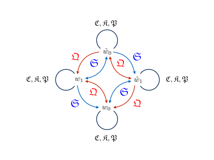
Figure 3: The 4-dimensional module of the centrally-extended algebra.

However, using the fact that

$$\mathfrak{Q}\mathfrak{S}|\tilde{w}_{0}\rangle=C|\tilde{w}_{0}\rangle+\frac{M}{2}|w_{0}\rangle\ , \mathfrak{Q}\mathfrak{S}|w_{0}\rangle=C|w_{0}\rangle+\frac{M}{2}|\tilde{w}_{0}\rangle\ ,$$ (2.45)

$$\mathfrak{S}\mathfrak{Q}|\tilde{w}_{0}\rangle=C|\tilde{w}_{0}\rangle-\frac{M}{2}|w_{0}\rangle\ , \mathfrak{S}\mathfrak{Q}|w_{0}\rangle=C|w_{0}\rangle-\frac{M}{2}|\tilde{w}_{0}\rangle\ ,$$ (2.46)

we see that defining the linear combinations

$$|\Phi_{\pm}\rangle=|w_{0}\rangle\pm|\tilde{w}_{0}\rangle\ ,$$ (2.47)

implies

$$\mathfrak{Q}\mathfrak{S}|\Phi_{\pm}\rangle=\big{(}C+\frac{M}{2}\big{)}|\Phi_{\pm}\rangle\ ,\qquad\mathfrak{S}\mathfrak{Q}|\Phi_{\pm}\rangle=\big{(}C-\frac{M}{2}\big{)}|\Phi_{\pm}\rangle\ .$$ (2.48)

Furthermore,

$$\mathfrak{Q}|\Phi_{\pm}\rangle=\mp\frac{2C\mp M}{M}|w_{1}\rangle\pm\frac{2P}{M}|\tilde{w}_{1}\rangle\ ,\qquad\mathfrak{S}|\Phi_{\pm}\rangle=\pm\frac{2C\pm M}{M}|\tilde{w}_{1}\rangle\mp\frac{2K}{M}|w_{1}\rangle\ .$$ (2.49)

Using the definition of $M$ (2.40) one can easily see that

$$\mathfrak{Q}|\Phi_{\pm}\rangle\propto\mathfrak{S}|\Phi_{\pm}\rangle\propto|\Psi_{\pm}\rangle\ ,$$ (2.50)

and hence the 4-dimensional representation we constructed is actually reducible and is formed of two 2-dimensional representations

$$\{|\Phi_{\pm}\rangle,|\Psi_{\pm}\rangle\}\ .$$ (2.51)

To conclude, let us briefly mention orthogonality. Here we will make use of the real form of the algebra given in eq. (2.12), and the assumption that $M$ is real. We then have

$$\langle\Phi_{\mp}|\Phi_{\pm}\rangle=\langle w_{0}|(\mathbf{1}+\frac{1}{M}([\mathfrak{Q},\mathfrak{S}]-[\mathfrak{Q},\mathfrak{S}]^{\dagger})-\frac{1}{M^{2}}[\mathfrak{Q},\mathfrak{S}]^{\dagger}[\mathfrak{Q},\mathfrak{S}]|w_{0}\rangle\ .$$ (2.52)

Using the conjugation relations we find that $[\mathfrak{Q},\mathfrak{S}]^{\dagger}=[\mathfrak{Q},\mathfrak{S}]$. Furthermore, as $[\mathfrak{Q},\mathfrak{S}]=2\mathfrak{C}-2\mathfrak{S}\mathfrak{Q}=-2\mathfrak{C}+2\mathfrak{Q}\mathfrak{S}$ we find

$$\begin{split}\langle\Phi_{\mp}|\Phi_{\pm}\rangle&=\langle w_{0}|\mathbf{1}+\frac{1}{M^{2}}(2\mathfrak{C}-2\mathfrak{S}\mathfrak{Q})(2\mathfrak{C}-2\mathfrak{Q}\mathfrak{S})|w_{0}\rangle=\langle w_{0}|\mathbf{1}-\frac{4}{M^{2}}(\mathfrak{C}^{2}-\mathfrak{P}\mathfrak{K})|w_{0}\rangle\\ &=(1-\frac{4(C^{2}-PK)}{M^{2}})\langle w_{0}|w_{0}\rangle=0\ .\end{split}$$ (2.53)

Therefore, the two representations are orthogonal.

This construction can then be straightforwardly applied to the 4-dimensional representation arising as the tensor product of two of the 2-dimensional irreps of section 2.2. Explicit details of this construction are given in appendix Appendix B: Decomposition of the tensor product of two 2-dimensional representations and will be particularly relevant for the scattering theory discussed in section 3. In particular, it implies that the S-matrix for the scattering of two of the 2-dimensional irreps is not completely fixed by symmetries up to an overall factor.

Let us finally make the important observation that the arguments of this section cannot be applied for the $M=0$ case (such as, for instance, the scattering of two massless particles with the momenta taken at the bound-state point ). In this case what we find is the analog of the projective indecomposable representation of section 2.1. In particular, one can check that, at $M=0$, the state $|\tilde{w}_{0}^{(0)}\rangle\equiv[\mathfrak{Q},\mathfrak{S}]|w_{0}\rangle$ is such that

$$\mathfrak{Q}\mathfrak{S}\,|\tilde{w}_{0}^{(0)}\rangle\,=\,\mathfrak{S}\mathfrak{Q}\,|\tilde{w}_{0}^{(0)}\rangle\,=\,C\,|\tilde{w}_{0}^{(0)}\rangle,\qquad\mathfrak{Q}\,|\tilde{w}_{0}^{(0)}\rangle\,\propto\,\mathfrak{S}\,|\tilde{w}_{0}^{(0)}\rangle,$$ (2.54)

where we have used $M^{2}=4(C^{2}-PK)=0$ to derive the last proportionality statement. However, this is the only state which satisfies these properties, meaning we do not have two solutions to these conditions (as we did in the $M\neq 0$ case above). Therefore, there is only one irreducible 2-dimensional block, containing the states $\{|\tilde{w}_{0}^{(0)}\rangle,\mathfrak{Q}|\tilde{w}_{0}^{(0)}\rangle\}$, and the 4-dimensional representation is reducible but not fully reducible (i.e. it is indecomposable).

3 S-matrix for massive modes of $\mathbf{AdS_{2}\times S^{2}}$

In this section we study the S-matrix for the massive modes of the light-cone gauge $AdS_{2}\times S^{2}\times T^{6}$ superstring. As mentioned in section 2 from the structure of the symmetry algebra and the integrability of the theory we expect the S-matrix for the massive fields $y$, $z$, $\zeta$ and $\chi$ to be constructed from the graded tensor product of two copies of an S-matrix describing the scattering of $1+1$ massive modes, $\phi$ and $\psi$. The former are defined in terms of the latter in (2.1).

The excitations $\phi$ and $\psi$ should transform in the massive representation of $\mathfrak{psu}(1|1)\ltimes\mathbb{R}^{3}$ discussed in section 2.2. Their S-matrix is then fixed by demanding invariance under this symmetry

$$\Delta^{op}(\mathfrak{J})\mathbb{S}=\mathbb{S}\Delta(\mathfrak{J})\ .$$ (3.1)

Accounting for conservation of the value of $(-1)^{F}$, where $F$ is the fermion number, the most general form for the S-matrix is

$$\mathbb{S}\left|\phi\phi^{\prime}\right>=S_{1}\left|\phi\phi^{\prime}\right>+Q_{1}\left|\psi\psi^{\prime}\right>\ ,\qquad\mathbb{S}\left|\psi\psi^{\prime}\right>=S_{2}\left|\psi\psi^{\prime}\right>+Q_{2}\left|\phi\phi^{\prime}\right>\ ,$$

$$\mathbb{S}\left|\phi\psi^{\prime}\right>=T_{1}\left|\phi\psi^{\prime}\right>+R_{1}\left|\psi\phi^{\prime}\right>\ ,\qquad\mathbb{S}\left|\psi\phi^{\prime}\right>=T_{2}\left|\psi\phi^{\prime}\right>+R_{2}\left|\phi\psi^{\prime}\right>\ ,$$ (3.2)

where $x^{\pm}$, $m$ are the kinematic variables associated to the first particle and $x^{\prime\pm}$, $m^{\prime}$ to the second particle, that is

$$x^{+}+\frac{1}{x^{+}}-x^{-}-\frac{1}{x^{-}}=\frac{2im}{{\rm h}}\ ,\qquad\quad x^{\prime+}+\frac{1}{x^{\prime+}}-x^{\prime-}-\frac{1}{x^{\prime-}}=\frac{2im^{\prime}}{{\rm h}}\ .$$ (3.3)

As a consequence of the discussion in section 2.3 this symmetry will only fix the S-matrix up to two arbitrary functions. One of these functions can be found by requiring the S-matrix also satisfies the Yang-Baxter equation along with additional physical requirements. There are four solutions to the Yang-Baxter equation, two of which we ignore as they violate crossing symmetry. The other two are related by a sign. To fix the sign, we demand that in the BMN limit (for details see section 3.2) the S-matrix reduces to the identity operator. The functions parametrizing the exact S-matrix (3.2) are then given by 

$$S_{1}=\sqrt{\frac{x^{+}x^{\prime-}}{x^{-}x^{\prime+}}}\frac{x^{-}-x^{\prime+}}{x^{+}-x^{\prime-}}\frac{1+s_{1}}{2}\mathcal{\tilde{P}}_{{}_{0}}\ , S_{2}=\frac{1+s_{2}}{2}\mathcal{\tilde{P}}_{{}_{0}}\ ,$$

$$T_{1}=\sqrt{\frac{x^{\prime-}}{x^{\prime+}}}\frac{x^{+}-x^{\prime+}}{x^{+}-x^{\prime-}}\frac{1+t_{1}}{2}\mathcal{\tilde{P}}_{{}_{0}}\ , T_{2}=\sqrt{\frac{x^{+}}{x^{-}}}\frac{x^{-}-x^{\prime-}}{x^{+}-x^{\prime-}}\frac{1+t_{2}}{2}\mathcal{\tilde{P}}_{{}_{0}}\ ,$$

$$\frac{Q_{1}}{\alpha\alpha^{\prime}}=\alpha\alpha^{\prime}\,Q_{2}=-\frac{i}{2}\,\sqrt[4]{\frac{x^{-}x^{\prime+}}{x^{+}x^{\prime-}}}\frac{\eta\eta^{\prime}}{x^{+}-x^{\prime-}}\frac{f}{x^{-}x^{\prime+}}\mathcal{\tilde{P}}_{{}_{0}}\ , \frac{\alpha^{\prime}}{\alpha}R_{1}=\frac{\alpha}{\alpha^{\prime}}R_{2}=-\frac{i}{2}\,\sqrt[4]{\frac{x^{+}x^{\prime-}}{x^{-}x^{\prime+}}}\frac{\eta\eta^{\prime}}{x^{+}-x^{\prime-}}\mathcal{\tilde{P}}_{{}_{0}}\ ,$$ (3.4)

where

$$f=\frac{\sqrt{\frac{x^{+}}{x^{-}}}(x^{-}-\frac{1}{x^{+}})-\sqrt{\frac{x^{\prime+}}{x^{\prime-}}}(x^{\prime-}-\frac{1}{x^{\prime+}})}{1-\frac{1}{x^{+}x^{-}x^{\prime+}x^{\prime-}}}\ ,\qquad s_{1}= \frac{1-\frac{1}{x^{+}x^{\prime-}}}{x^{-}-x^{\prime+}}f\ ,\qquad s_{2}=\frac{1-\frac{1}{x^{-}x^{\prime+}}}{x^{+}-x^{\prime-}}f\ ,$$ (3.5)

$$t_{1}= \frac{1-\frac{1}{x^{-}x^{\prime-}}}{x^{+}-x^{\prime+}}f\ ,\qquad t_{2}=\frac{1-\frac{1}{x^{+}x^{\prime+}}}{x^{-}-x^{\prime-}}f\ .$$ (3.6)

$\mathcal{\tilde{P}}_{{}_{0}}$ is an overall factor that sits outside the matrix structure and is not fixed by symmetries or the Yang-Baxter equation. Let us emphasize that, as discussed beneath eq. (2.27), when written in these variables the S-matrix is independent of $m$ and $m^{\prime}$, which can take any value. The limits $m\to 0$ and $m^{\prime}\to 0$ are subtle however, and will be discussed in detail in section 5. Let us also note that if we take $\alpha$ to be given by (2.33), which is the choice suitable for string theory, then $Q_{1}=Q_{2}$ and $R_{1}=R_{2}$. From now on we will take $\alpha$ to be given by this value.

The S-matrix (3) can be thought of as a $4\times 4$ block diagonal matrix

$$\left(\begin{array}[]{cccc}S_{1}&Q_{1}&0&0\\ Q_{2}&S_{2}&0&0\\ 0&0&T_{1}&R_{1}\\ 0&0&T_{2}&R_{2}\end{array}\right)\ .$$ (3.7)

One can then check that each of the two $2\times 2$ blocks have equal trace and determinant,

$$S_{1}+S_{2}=T_{1}+T_{2}\ ,\qquad S_{1}S_{2}-Q_{1}Q_{2}=T_{1}T_{2}-R_{1}R_{2}\ .$$ (3.8)

The second of these equations is particularly important as it implies the tensor product of two copies of the S-matrix possesses an additional $U(1)$ symmetry, which will be discussed further in section 6 and appendix Appendix A: Expansion of tensor product and $\mathbf{U(1)}$ symmetry.

For completeness let us note that the two solutions that violate crossing symmetry are given by $f=0$ and $f\to\infty$ (for the latter one should first rescale $\mathcal{\tilde{P}}_{{}_{0}}$ by $f^{-1}$ and then take $f\to\infty$). As $\phi$ and $\psi$ are real and the charge conjugation matrix diagonal, which will be demonstrated in the next section (cf. (3.23)), the two processes

$$\phi\,\phi\to\psi\,\psi\qquad\text{and}\qquad\phi\,\psi\to\psi\,\phi\ ,$$ (3.9)

should be related by a crossing transformation. However, if $f$ vanishes then so does the amplitude for the first of these processes, but not for the second. Similarly, if $f\to\infty$ then the amplitude for the second process vanishes, but not for the first. Consequently, in both cases the two processes cannot be related by a crossing transformation and hence there is a violation of crossing symmetry as claimed.

It is interesting to note that taking $f=0$ and $f\to\infty$ we recover the massive S-matrices of the $AdS_{3}\times S^{3}\times T^{4}$ light-cone gauge superstring [21, 22]. The symmetry is enhanced accordingly from $\mathfrak{psu}(1|1)\ltimes\mathbb{R}^{3}$ to $[\mathfrak{u}(1)\inplus\mathfrak{psu}(1|1)^{2}]\ltimes\mathfrak{u}(1)\ltimes\mathbb{R}^{3}$. For the $AdS_{3}\times S^{3}\times T^{4}$ light-cone gauge-fixed theory there is no issue with crossing symmetry as the fields are complex. Therefore, the individual S-matrices do not map to themselves under the crossing transformation, rather to a different S-matrix with the crossed particle replaced by its antiparticle. Finally let us also point out that the S-matrix relevant for the $AdS_{2}\times S^{2}\times T^{6}$ light-cone gauge superstring, see eqs. (3) and (3.4), is a linear combination, with coefficients depending on $x^{\pm}$ and $x^{\prime\pm}$, of the $f=0$ and $f\to\infty$ S-matrices. It is non-trivial that such a combination exists with unitarity, crossing symmetry and the Yang-Baxter equation all satisfied.

3.1 The overall factor and crossing symmetry

As currently written the factor $\mathcal{\tilde{P}}_{{}_{0}}$ is neither a phase factor or antisymmetric. Indeed, given the reality conditions $(x^{\pm})^{*}=x^{\mp}$ and $(x^{\prime\pm})^{*}=x^{\mp}$, the functions $f$, $s_{1,2}$ and $t_{1,2}$ satisfy the following relations:

$$f^{*} =f\ ,\qquad s_{1,2}^{*} =s^{\vphantom{*}}_{2,1}\ ,\qquad t_{1,2}^{*} =t^{\vphantom{*}}_{2,1}\ ,$$ (3.10)

$$f(x^{\prime},x) =-f(x^{\prime},x)\ ,\qquad s_{1,2}(x^{\prime},x) =s_{2,1}(x,x^{\prime})\ ,\qquad t_{1,2}(x^{\prime},x) =t_{1,2}(x,x^{\prime})\ .$$ (3.11)

Notice that, if we consider the $m=m^{\prime}$ case, then on-shell (i.e. when the dispersion relations (3.3) are satisfied) we have $t_{1}\approx t_{2}$. Given the reality conditions, this means in particular that $t_{1},t_{2}$ are real.

Based on this, and as a consequence of braiding and QFT unitarity, the overall factor should satisfy 

$$\mathcal{\tilde{P}}_{{}_{0}}\mathcal{\tilde{P}}_{{}_{0}}^{*}=\mathcal{\tilde{P}}_{{}_{0}}(x,x^{\prime})\mathcal{\tilde{P}}_{{}_{0}}(x^{\prime},x)=\frac{4(x^{-}-x^{\prime+})(x^{+}-x^{\prime-})}{(x^{+}-x^{\prime+})(x^{-}-x^{\prime-})(1+t_{1})(1+t_{2})-(x^{+}-x^{-})(x^{\prime+}-x^{\prime-})}{\color[rgb]{0,0,0}\equiv N(x,x^{\prime})}\ .$$ (3.12)

To isolate an antisymmetric phase factor, we can define $\mathcal{P}_{{}_{0}}$ as follows:

$$\mathcal{P}_{{}_{0}}=\det\bigg{(}\begin{array}[]{cc}S_{1}&Q_{1}\\ Q_{2}&S_{2}\end{array}\bigg{)}=\det\bigg{(}\begin{array}[]{cc}T_{1}&R_{1}\\ R_{2}&T_{2}\end{array}\bigg{)}\ {\color[rgb]{0,0,0}\equiv\,\exp{{\color[rgb]{0,0,0}i}\theta(x,x^{\prime})}},$$ (3.13)

where $\theta(x,x^{\prime})$ is an antisymmetric phase shift, i.e. $\theta(x,y)=-\theta(y,x)$, and the second equality follows from eq. (3.8). We then have that $\mathcal{P}_{{}_{0}}$ is proportional to $\mathcal{\tilde{P}}_{{}_{0}}^{2}$, and hence is a natural phase to consider recalling that the full S-matrix for the massive modes is given by the tensor product of two of the factor S-matrices (3). As claimed the unitarity conditions for $\mathcal{P}_{{}_{0}}$ are then

$$\mathcal{P}_{{}_{0}}\mathcal{P}_{{}_{0}}{}^{\!*}=\mathcal{P}_{{}_{0}}(x,x^{\prime})\mathcal{P}_{{}_{0}}(x^{\prime},x)=1\ .$$ (3.14)

Crossing symmetry provides an additional constraint on the overall factor $\mathcal{\tilde{P}}_{{}_{0}}$, which takes the form

$$\mathcal{\tilde{P}}_{{}_{0}}{\color[rgb]{0,0,0}(x^{\prime},\bar{x})}=s_{2}{\color[rgb]{0,0,0}(x,x^{\prime})}\,\mathcal{\tilde{P}}_{{}_{0}}{\color[rgb]{0,0,0}(x,x^{\prime})}\ ,$$ (3.15)

where the “crossed” Zhukovsky variables $\bar{x}^{\pm}$ are, as usual, given by

$$\bar{x}^{\pm}=\frac{1}{x^{\pm}}\ ,$$ (3.16)

corresponding to $\bar{e}=-e$ and $\bar{\textrm{p}}=-\textrm{p}$. It is useful to note that we have the following identities

$$s_{1,2}{\color[rgb]{0,0,0}(x^{\prime},\bar{x})}=s_{1,2}^{-1}{\color[rgb]{0,0,0}(x,x^{\prime})}\ ,\qquad t_{1,2}{\color[rgb]{0,0,0}(x^{\prime},\bar{x})}=t_{2,1}^{-1}{\color[rgb]{0,0,0}(x,x^{\prime})}\ .$$ (3.17)

Using the braiding unitarity relation (3.12) it is simple to recast (3.15) in the more familiar form

$$\mathcal{\tilde{P}}_{{}_{0}}{\color[rgb]{0,0,0}(x,x^{\prime})}\mathcal{\tilde{P}}_{{}_{0}}{\color[rgb]{0,0,0}(\bar{x},x^{\prime})}=\frac{N(\bar{x},x^{\prime})}{s_{2}(x,x^{\prime})}\ .$$ (3.18)

This relation then translates to the following rather complicated constraint for the antisymmetric phase factor $\mathcal{P}_{{}_{0}}$

$$\mathcal{P}_{{}_{0}}{\color[rgb]{0,0,0}(x,x^{\prime})}\mathcal{P}_{{}_{0}}{\color[rgb]{0,0,0}(\bar{x},x^{\prime})}=\frac{S_{1}S_{2}-Q_{1}Q_{2}}{S_{1}S_{2}+R_{1}R_{2}}=\frac{T_{1}T_{2}-R_{1}R_{2}}{T_{1}T_{2}+Q_{1}Q_{2}}\equiv f_{2}{\color[rgb]{0,0,0}(x,x^{\prime})}\ ,$$ (3.19)

and hence it appears that we either have a simple crossing relation or simple unitarity relations.

Using Hopf algebra arguments, we have checked that crossing symmetry is present for the representation of interest for any value of $m$ and $m^{\prime}$. Denoting the symmetry algebra as $\cal{A}$, the antipode $\Sigma$ is found from the defining rule

$$\mu\,(\Sigma\otimes\mathbf{1})\,\Delta=\eta\,\epsilon\ ,$$ (3.20)

where $\mu$ is the multiplication map, $\eta:\mathbb{C}\to{\cal{A}}$ is the unit and $\epsilon:{\cal{A}}\to\mathbb{C}$ is the counit, which annihilates all generators apart from $\mathbf{1}$ and $e^{i\textrm{p}}$ (acting on which, it returns $1$). The antipode being a Lie algebra anti-homomorphism, we simply need to derive

$$\Sigma(\mathfrak{Q})=-e^{-i\frac{\textrm{p}}{2}}\mathfrak{Q},\qquad\Sigma(\mathfrak{Q})=-e^{i\frac{\textrm{p}}{2}}\mathfrak{G},\qquad\Sigma(\mathbf{1})=\mathbf{1},\qquad\Sigma(e^{i\textrm{p}})=e^{-i\textrm{p}}\ .$$ (3.21)

This map is idempotent and therefore equal to its inverse. We impose

$$\Sigma\big{(}\mathfrak{J}(x^{\pm})\big{)}=\mathscr{C}^{-1}\bigg{[}\mathfrak{J}\bigg{(}\frac{1}{x^{\pm}}\bigg{)}\bigg{]}^{{\color[rgb]{0,0,0}st}}\mathscr{C}\ ,$$ (3.22)

where $\mathscr{C}$ is the charge conjugation matrix

$$\mathscr{C}=\begin{pmatrix}1&0\\ 0&i\end{pmatrix}\ ,$$ (3.23)

and the label ^st denotes supertransposition. The fundamental crossing relation for an abstract R-matrix  is then given by (cf. [24])

$$(\Sigma\otimes\mathbf{1})R=R^{-1}=(\mathbf{1}\otimes\Sigma^{-1})R\ ,$$ (3.24)

which projects into the representation of interest as

$$(\mathscr{C}^{-1}\otimes\mathbf{1})\mathbb{S}^{{\color[rgb]{0,0,0}st}_{1}}(\bar{x},x^{\prime})(\mathscr{C}\otimes\mathbf{1})\mathbb{S}(x,x^{\prime})=\mathbf{1}\otimes\mathbf{1}\ ,$$ (3.25)

and an analogous equation for the second factor. Here ${}^{{\color[rgb]{0,0,0}st}_{i}}$ denotes the supertranspose for factor $i$, and we are using the Hopf algebra convention for the S-matrix crossing [24] (see [3] for the convention used in the field theory literature). The S-matrix (3.2) with parametrizing functions (3.4) satisfies this relation provided the overall factor satisfies the crossing equation given in (3.15).

It is important to note that the crossing equations given above are somewhat formal as we have not specified a path on the rapidity plane. To specify such a path we would need to know the precise form of the dispersion relation, and hence its uniformization. In particular, there is still the logical possibility that $m$ and $m^{\prime}$ are themselves momentum-dependent functions (which should be invariant under crossing). This possibility would not alter the analysis we have performed so far. In the scenario that $m$ and $m^{\prime}$ are non-vanishing and constant the dispersion relation becomes the same as in the $AdS_{5}\times S^{5}$ light-cone gauge string theory and the analytic continuation should be the same as in that case [24, 38, 39].

In spite of our lack of knowledge of the complete dispersion relation, one thing we can investigate is double crossing [24]. In particular, the left-hand sides of (3.18) and (3.19) are symmetric under $x\leftrightarrow\bar{x}$, however the right-hand sides are not. This asymmetry encodes the fact that the overall factor should not be a meromorphic function of the parameters that uniformize the dispersion relation (generalized rapidities). Furthermore, as a consistency check, one can confirm that the following equality holds true:

$${\color[rgb]{0,0,0}\Omega(x,x^{\prime})\,\equiv\,\frac{\mathcal{\tilde{P}}_{{}_{0}}^{2}(x,x^{\prime})}{\mathcal{\tilde{P}}_{{}_{0}}^{2}(\bar{\bar{x}},x^{\prime})}\ .\ \frac{\mathcal{P}_{{}_{0}}(\bar{\bar{x}},x^{\prime})}{\mathcal{P}_{{}_{0}}(x,x^{\prime})}=\,\left(\frac{N(\bar{x},x^{\prime})}{s_{2}(x,x^{\prime})}\right)^{2}\ .\ \left(\frac{s_{2}(\bar{x},x^{\prime})}{N(x,x^{\prime})}\right)^{2}\ .\ \frac{f_{2}(\bar{x},x^{\prime})}{f_{2}{\color[rgb]{0,0,0}(x,x^{\prime})}}\,=\,1\ .}$$ (3.26)

This is obtained by comparing the ratio of the right-hand side of (3.18) (squared) to the same quantity with $x\to\bar{x}$, against the corresponding ratio for the right-hand side of (3.19). The fact that $\Omega=1$ confirms that $\mathcal{\tilde{P}}_{{}_{0}}^{2}$ and $\mathcal{P}_{{}_{0}}$ differ only by a factor that behaves like a rational function under double crossing, as is expected.

It is easy to convince oneself that the ratio $\frac{f_{2}(\bar{x},x^{\prime})}{f_{2}{\color[rgb]{0,0,0}(x,x^{\prime})}}$ encodes the discontinuity of the overall S-matrix factor across branch cuts in the, as yet unknown, rapidity plane. It is of interest to note that this ratio differs from the corresponding one in the $AdS_{5}\times S^{5}$ case, suggesting that the analytic structure of the $AdS_{2}\times S^{2}$ light-cone gauge-fixed theories is not the same. To understand crossing symmetry and the phase in more detail clearly requires a deeper knowledge of the dispersion relation, which, as it is not entirely fixed by symmetries, we leave for future investigation.

3.2 Comparison with perturbation theory

Defining the effective string tension

$$h=\frac{R^{2}}{2\pi\alpha^{\prime}}\ ,$$ (3.27)

the tree-level S-matrix for the scattering of massive modes in the light-cone gauge $AdS_{2}\times S^{2}\times T^{6}$ superstring following from near-BMN perturbation theory can be be found by suitably truncating the corresponding result for $AdS_{5}\times S^{5}$ or $AdS_{3}\times S^{3}\times T^{4}$ [28] (various components were also computed in [17]). This gives

$$S_{1}= \ 1+\frac{i}{4h}\big{[}(1-2{\rm a})(e^{\prime}p-ep^{\prime})+l_{1}\big{]}+\mathcal{O}(\frac{1}{h^{2}})\ ,$$

$$S_{2}= \ 1+\frac{i}{4h}\big{[}(1-2{\rm a})(e^{\prime}p-ep^{\prime})-l_{1}\big{]}+\mathcal{O}(\frac{1}{h^{2}})\ ,$$

$$T_{1}= \ 1+\frac{i}{4h}\big{[}(1-2{\rm a})(e^{\prime}p-ep^{\prime})-l_{2}\big{]}+\mathcal{O}(\frac{1}{h^{2}})\ ,$$

$$T_{2}= \ 1+\frac{i}{4h}\big{[}(1-2{\rm a})(e^{\prime}p-ep^{\prime})+l_{2}\big{]}+\mathcal{O}(\frac{1}{h^{2}})\ ,$$

$$Q_{1}= \ Q_{2}=\frac{i}{2h}l_{3}+\mathcal{O}(\frac{1}{h^{2}})\ ,\qquad R_{1}=R_{2}=-\frac{i}{2h}l_{4}+\mathcal{O}(\frac{1}{h^{2}})\ ,$$ (3.28)

where the functions $l_{i}$ are defined as

$$l_{1}(p,p^{\prime})= \frac{p^{2}+p^{\prime 2}}{e^{\prime}p-ep^{\prime}}\ ,\qquad\qquad l_{2}(p,p^{\prime})=\frac{p^{2}-p^{\prime 2}}{e^{\prime}p-ep^{\prime}}\ ,$$

$$l_{3}(p,p^{\prime})= -\frac{pp^{\prime}}{2(e^{\prime}p-ep^{\prime})}\big{[}\sqrt{(e+p)(e^{\prime}-p^{\prime})}-\sqrt{(e-p)(e^{\prime}+p^{\prime})}\big{]}\ ,$$

$$l_{4}(p,p^{\prime})= -\frac{pp^{\prime}}{2(e^{\prime}p-ep^{\prime})}\big{[}\sqrt{(e+p)(e^{\prime}-p^{\prime})}+\sqrt{(e-p)(e^{\prime}+p^{\prime})}\big{]}\ .$$

The parameter ${\rm a}$ is the standard gauge-fixing parameter of the uniform light-cone gauge [14]. In [17] it was shown that to one-loop the near-BMN dispersion relation is given by

$$e^{2}=1+p^{2}+\mathcal{O}(h^{-2})\ .$$ (3.29)

The one-loop near-BMN result can be constructed via unitarity methods following [40]. As expected from unitarity methods, this will certainly give the correct logarithmic terms in the one-loop S-matrix, and indeed this has already been argued in [17]. However, the prescription given in [40] is also conjectured to give the correct rational terms for integrable theories. Under this assumption we find that the one-loop S-matrix takes the following form

$$S_{1}= \ \exp\big{\{}\frac{i}{4h}(1-2{\rm a})(e^{\prime}p-ep^{\prime})\big{\}}\ \sigma_{AdS_{2}}\ \big{[}1+\frac{i}{4h}l_{1}-\frac{\ell}{32h^{2}}\,\big{]}+\mathcal{O}(\frac{1}{h^{3}})\ ,$$

$$S_{2}= \ \exp\big{\{}\frac{i}{4h}(1-2{\rm a})(e^{\prime}p-ep^{\prime})\big{\}}\ \sigma_{AdS_{2}}\ \big{[}1-\frac{i}{4h}l_{1}-\frac{\ell}{32h^{2}}\,\big{]}+\mathcal{O}(\frac{1}{h^{3}})\ ,$$

$$T_{1}= \ \exp\big{\{}\frac{i}{4h}(1-2{\rm a})(e^{\prime}p-ep^{\prime})\big{\}}\ \sigma_{AdS_{2}}\ \big{[}1-\frac{i}{4h}l_{2}-\frac{\ell}{32h^{2}}\,\big{]}+\mathcal{O}(\frac{1}{h^{3}})\ ,$$

$$T_{2}= \ \exp\big{\{}\frac{i}{4h}(1-2{\rm a})(e^{\prime}p-ep^{\prime})\big{\}}\ \sigma_{AdS_{2}}\ \big{[}1+\frac{i}{4h}l_{2}-\frac{\ell}{32h^{2}}\,\big{]}+\mathcal{O}(\frac{1}{h^{3}})\ ,$$

$$Q_{1}= \ Q_{2}=\exp\big{\{}\frac{i}{4h}(1-2{\rm a})(e^{\prime}p-ep^{\prime})\big{\}}\ \sigma_{AdS_{2}}\ \big{[}\frac{i}{2h}l_{3}\,\big{]}+\mathcal{O}(\frac{1}{h^{3}})\ ,$$

$$R_{1}= \ R_{2}=\exp\big{\{}\frac{i}{4h}(1-2{\rm a})(e^{\prime}p-ep^{\prime})\big{\}}\ \sigma_{AdS_{2}}\ \big{[}-\frac{i}{2h}l_{4}\,\big{]}+\mathcal{O}(\frac{1}{h^{3}})\ ,$$ (3.30)

where the expansion of the phase factor $\sigma_{AdS_{2}}$ is given by

$$\begin{split}\sigma_{AdS_{2}}=\exp\big{\{}&\frac{i}{8\pi\,h^{2}}\frac{p^{2}p^{\prime}{}^{2}\big{(}(e^{\prime}p-ep^{\prime})-(ee^{\prime}-pp^{\prime})\operatorname{arsinh}[e^{\prime}p-ep^{\prime}]\big{)}}{(e^{\prime}p-ep^{\prime})^{2}}+\mathcal{O}(\frac{1}{h^{3}})\big{\}}\ ,\end{split}$$ (3.31)

while

$$\ell=\frac{p^{4}+p^{\prime}{}^{4}+2p^{2}p^{\prime}{}^{2}(ee^{\prime}-pp^{\prime})}{(e^{\prime}p-ep^{\prime})^{2}}\ ,$$ (3.32)

is fixed by the requirement of unitarity. As observed in [17] the one-loop logarithms are consistent with the one-loop phase being related to the Hernandez-Lopez phase [26].

We define the near-BMN expansion of the exact result as follows

$$\begin{split}&\textrm{e}=e\ ,\qquad m=\rho_{3}+\rho_{4}h^{-1}+\mathcal{O}(h^{-2})\ ,\qquad\textrm{p}=\frac{p}{h\big{(}\rho_{5}+\rho_{6}h^{-1}+\mathcal{O}(h^{-2})\big{)}}\ ,\\ &{\rm h}=h\big{(}\rho_{1}+\rho_{2}h^{-1}+\mathcal{O}(h^{-2})\big{)}\ ,\end{split}$$ (3.33)

and similarly for $\textrm{e}^{\prime},\textrm{p}^{\prime}$ and $m^{\prime}$. Here for generality we have allowed for various rescalings, however, for simplicity we will assume that the $\rho_{i}$ are constants.

Let us remark that in this paper we are considering the $AdS_{2}\times S^{2}\times T^{6}$ background supported by Ramond-Ramond fluxes [12], and hence the light-cone gauge-fixed theory should be parity invariant [16, 17]. Therefore, if it were the case that $m$ receives quantum corrections depending on the momentum they should respect the corresponding constraint. This is in contrast to backgrounds partially (or wholly) supported by Neveu-Schwarz flux, for which $m$ may have a dependence on $p$ that breaks parity (see, for example, [41] for discussions of the dispersion relation of the $AdS_{3}\times S^{3}\times T^{4}$ light-cone gauge-fixed theory supported by a mix of fluxes). It is worth noting that the $AdS_{2}\times S^{2}\times T^{6}$ background can also be supported by a mixture of Ramond-Ramond and Neveu-Schwarz fluxes [4] and it would be interesting to see how the presence of the latter affects the representations discussed in this paper.

Expanding the exact dispersion relation (2.31) in the near-BMN regime, we recover (3.29) if we take

$$\rho_{5}=\rho_{1}\ ,\qquad\rho_{6}=\rho_{2}\ ,\qquad\rho_{3}=1\ ,\qquad\rho_{4}=0\ .$$ (3.34)

Further expanding the exact S-matrix (3.4) in the near-BMN regime, taking $\alpha$ given by (2.33), and fixing the overall factor $\mathcal{\tilde{P}}_{{}_{0}}$ such that any one of the eight amplitudes agrees with perturbation theory, we find that, so long as

$$\rho_{1}=1\ ,$$ (3.35)

the remaining seven also agree with perturbation theory, (3.28) and (3.30).

4 Yangian symmetry

4.1 Massive case

In this section we would like to discuss the issue of Yangian symmetry. The first observation is that, in the massive case (we can fix $m=m^{\prime}=1$ for the purposes of this section), we could not apply the same standard Yangian symmetry of the R-matrix which works for the massless case (see section 4.2). The massive representation is a long one (cf. section 2.2), and a similar result was found for long representations of $\mathfrak{psu}(2|2)\ltimes\mathbb{R}^{3}$ [29]. The long representations studied in [29] bear a strong resemblance to the ones in this paper, up to the different dimensionality.

We proceed by postulating the commutation relations of the standard $\mathfrak{sl}(1|1)$ Yangian in Drinfeld’s second realization [42, 43] (with central extensions)

$$\begin{gathered}\{\mathfrak{e}_{m},\mathfrak{f}_{n}\}=-\mathfrak{h}_{m+n}\ ,\qquad\{\mathfrak{e}_{m},\mathfrak{e}_{n}\}=\mathfrak{p}_{m+n}\ ,\qquad\{\mathfrak{f}_{m},\mathfrak{f}_{n}\}=\mathfrak{p}_{m+n}^{\dagger}\ ,\qquad[\mathfrak{h}_{m},\cdot]=[\mathfrak{p}_{m},\cdot]=[\mathfrak{p}_{m}^{\dagger},\cdot]=0\ .\\ \end{gathered}$$ (4.1)

One can check that the coproducts obtained from

$$\Delta({\mathfrak{e}}_{1}) =\mathfrak{e}_{1}\otimes\mathbf{1}+e^{i\frac{\textrm{p}}{2}}\otimes\mathfrak{e}_{1}+\mathfrak{h}_{0}\,e^{i\frac{\textrm{p}}{2}}\otimes\mathfrak{e}_{0}\ ,$$ (4.2)

$$\Delta(\mathfrak{f}_{1}) =\mathfrak{f}_{1}\otimes\mathbf{1}+e^{-i\frac{\textrm{p}}{2}}\otimes\mathfrak{f}_{1}+\mathfrak{f}_{0}\otimes\mathfrak{h}_{0}\ ,$$

and their opposites satisfy the defining relations (4.1) and hence provide homomorphisms of the Yangian. The antipode $\Sigma$ can be easily found from (4.2) using the defining property

$$\mu\,(\Sigma\otimes\mathbf{1})\,\Delta=\eta\,\epsilon\ ,$$ (4.3)

where $\epsilon$ annihilates all level $1$ generators. Combined, this defines the Hopf algebra structure of the standard Yangian.

One can construct a family of representations of the Yangian (4.2) starting from a slightly simpler level-zero (Lie algebra) representation compared to the one we use in section 2.2. Determining the level $1$ generators in this representation, we can obtain all the central elements up to and including level $2$, together with their coproducts and opposite coproducts. Following the strategy of [29], one can check whether all the central coproducts are co-commutative, as this is a necessary condition for the existence of an R-matrix scattering two such representations (see footnote 1). We found that

$$\Delta^{op}(\mathfrak{p}_{2})\neq\Delta(\mathfrak{p}_{2})\ ,$$ (4.4)

for all members of the family of representations. This implies that at least one representation of the standard Yangian does not admit an R-matrix, excluding the existence of a universal R-matrix.

However, it is likely that the massive R-matrix may admit a coproduct which is not precisely the same as for massless representations, but still of the type found in [44]. Moreover, considerations as in footnote 3 of [29] are likely to apply. We leave this investigation for future work.

4.2 Massless case

The situation is different for the massless limit $m=m^{\prime}=0$ (see the discussion at the beginning of section 5). In this case, in the absence of the central extensions ($b=c=0$, i.e. considering again the $\mathfrak{gl}(1|1)$ algebra), the representation would become one of the reducible but indecomposable modules of section 2.1. In fact, in that case the condition $m=ad-bc=ad=0$ would force one of the fermionic generators to be identically zero. The indecomposable would then be made up of short 1-dimensional $\mathfrak{gl}(1|1)$ irreps. This suggests that the Yangian might now be straightforwardly derived from the standard one.

The fact that $m=0$ effectively works as a shortening condition, and the consequence that this allows for the existence of a Yangian representation, gives us significant encouragement that $m=0$ might be protected against quantum corrections in the full theory. This is also corroborated by explicit perturbative results, which have not yet found any evidence for a quantum lift of this condition (see, for instance, [12, 16]). Moreover, the subgroup of $SO(6)$ controlling the symmetry of the massless sector might allow one to construct a mechanism protecting the $m=0$ condition, analogous to the one described in [31] for $AdS_{3}\times S^{3}\times T^{4}$.

Indeed, this time we construct an evaluation representation of the Yangian (4.2)

$$\mathfrak{e}_{1}=u\,\mathfrak{e}_{0}\,=\,u\,\mathfrak{Q}\ ,\qquad\mathfrak{f}_{1}=u\,\mathfrak{f}_{0}\,=\,u\,\mathfrak{G}\ ,\qquad u=\frac{i{\rm h}}{x^{-}}\ ,$$ (4.5)

starting from the level $0$ one we consider in section 2.2, specializing to $m=0$. Due to the additional parameters compared to the $\mathfrak{gl}(1|1)$ case, the representation remains generically irreducible. Nevertheless, the obstruction encountered in the massive case is no longer present, i.e. all central charges we can build are co-commutative and in fact the R-matrix (for $m=m^{\prime}=0$) can be shown to be invariant under the standard Yangian. This is reminiscent of the $AdS_{5}\times S^{5}$ case, where the Yangian for short representations does not directly transfer to long ones as it stands [44, 45].

The crossing symmetry transformation reveals an interesting property, related to what was observed in [21] for the case of $AdS_{3}\times S^{3}\times T^{4}$, namely the existence of two different Yangian spectral (evaluation) parameters for the particle and the anti-particle representations. Here, the difference is superficial, as the massless condition makes the two spectral parameters coincide. In fact, the antipode obtained from applying (4.3) reads

$$\Sigma(\mathfrak{e}_{1})=-e^{-i\frac{\textrm{p}}{2}}\,(\mathfrak{e}_{1}+\mathfrak{e}_{0}\,\mathfrak{h}_{0})\ ,\qquad\Sigma(\mathfrak{f}_{1})=-e^{i\frac{\textrm{p}}{2}}\,(\mathfrak{f}_{1}+\mathfrak{f}_{0}\,\mathfrak{h}_{0})\ .$$ (4.6)

This effectively amounts to a shift in the spectral parameter $u$ by one of the central elements. When plugging this into the relation

$$\Sigma\big{(}{\mathfrak{j}_{1}}(x^{\pm})\big{)}=\mathscr{C}^{-1}\bigg{[}{\mathfrak{j^{a}}_{1}}\bigg{(}\frac{1}{x^{\pm}}\bigg{)}\bigg{]}^{{\color[rgb]{0,0,0}st}}\mathscr{C}\ ,$$ (4.7)

and postulating that the anti-particle representation is also of evaluation type, that is

$$\mathfrak{e^{a}}_{1}=u_{a}\,\mathfrak{Q}\ ,\qquad\mathfrak{f^{a}}_{1}=u_{a}\,\mathfrak{G}\ ,$$ (4.8)

we see that the conditions (4.7) and (4.6) reduce to the same equation that holds true for the level $0$ charges, i.e. (3.22), provided that the anti-particle spectral parameter is chosen to be

$$u_{a}=i{{\rm h}}\,x^{+}\ .$$ (4.9)

For massless particles,

$$u=u_{a}\ .$$ (4.10)

5 S-matrix for massless modes

In this section we investigate the $m\to 0$ and $m^{\prime}\to 0$ limits of the S-matrix constructed in section 3. From the dispersion relation (2.31) and under the assumption of constant $m$ and $m^{\prime}$, we may consider it natural to interpret these as massless limits.

While in principle these limits are already of interest in their own right, given the Yangian symmetry discussed in section 4.2, the resulting S-matrices may also be relevant for the scattering of massless modes in the $AdS_{2}\times S^{2}\times T^{6}$ light-cone gauge string theory. Indeed, for the $AdS_{3}\times S^{3}\times T^{4}$ light-cone gauge-fixed theory the massless modes transformed in the same type of representations as the massive modes (with vanishing mass and up to a suitable identification of highest weight states) [31]. Motivated by this, one may conjecture that the S-matrices constructed below can be used to build the S-matrices describing scattering processes involving massless modes (under the assumption that they remain massless and $m$ and $m^{\prime}$ remain zero at a quantum level – see the discussion below (LABEL:annn) and footnote 9) in the $AdS_{2}\times S^{2}\times T^{6}$ light-cone gauge superstring.

5.1 Derivation from Yangian invariance

The S-matrix describing the scattering of two massless excitations can be directly obtained by imposing Lie algebra and Yangian invariance for two $m=0$ representations of section 2.2, or as an $m,m^{\prime}\to 0$ limit of the massive S-matrix. In the latter case, one has to treat various $\frac{0}{0}$ limiting expressions, which come from the function $f$ in eq. (3.5). Taking care when resolving these singular limits we find agreement with the result from imposing Yangian invariance. In the massless limit the dispersion relation in terms of the Zhukovsky variables takes the form [31]

$$x^{+}=\frac{1}{x^{-}}\ .$$ (5.1)

In terms of the energy and momenta this translates to

$$\textrm{e}^{2}=4{\rm h}^{2}\sin^{2}\frac{\textrm{p}}{2}\qquad\Rightarrow\qquad\textrm{e}=2{\rm h}\,\big{|}\sin\frac{\textrm{p}}{2}\big{|}\ ,$$ (5.2)

and hence there are two branches of the dispersion relation depending on the sign of $\sin\frac{\textrm{p}}{2}$ [31]

$$x^{+}=\, \sigma e^{i\,\frac{\textrm{p}}{2}}\ ,\quad x^{-}=\frac{1}{x^{+}}\ ,\quad\sigma=\pm 1\ ,\qquad\qquad x^{\prime+}=\,\sigma^{\prime}e^{i\,\frac{\textrm{p}^{\prime}}{2}}\ ,\quad x^{\prime-}=\frac{1}{x^{\prime+}}\ ,\quad\sigma^{\prime}=\pm 1\ .$$ (5.3)

In the following we will use the convention that $\sigma=+1$ corresponds to a particle moving from left spatial infinity to right spatial infinity, i.e. right-moving, while $\sigma=-1$ corresponds to a left-moving particle.

Although the doubly-branched dispersion relation $\textrm{e}=2{\rm h}|\sin\frac{\textrm{p}}{2}|$ is non-relativistic, there are some similarities with the kinematics of massless relativistic scattering. Following [46], in the relativistic case one has

$$e=\,\frac{m_{0}}{2}\,e^{u}\ ,\qquad p=\,\pm\frac{m_{0}}{2}\,e^{u},\qquad m_{0},\,u\in\mathbb{R}\ .$$ (5.4)

A boost sends the rapidity $u\to u+\lambda$, with $\lambda\in\mathbb{R}$, hence the two branches can never be connected by such a transformation. In the non-relativistic case we have the two branches

$$\frac{i\,\textrm{e}}{{\rm h}}\,=\,\Big{[}x^{+}-\frac{1}{x^{+}}\Big{]}\ ,\qquad\textrm{p}=-2i\log x^{+}\in[0,\pi]\ ,$$

$$\frac{i\,\textrm{e}}{{\rm h}}\,=\,\Big{[}x^{+}-\frac{1}{x^{+}}\Big{]}\ ,\qquad\textrm{p}=-2i\log(-x^{+})\in[-\pi,0]\ ,$$ (5.5)

with $x^{+}$ a pure phase for real momentum and energy. As the S-matrix is not of difference form there is a priori no notion of boosts and hence it is not clear if the presence of two branches represents an obstruction to interpreting the $\sigma=\sigma^{\prime}=\pm 1$ scattering. However, as pointed out in [31], while the small momentum dispersion relation is relativistic, for the exact non-relativistic dispersion relation, the group velocity ${\rm v}=\frac{\partial\textrm{e}}{\partial\textrm{p}}$ is a non-trivial function of p and hence one may hope to give a physical interpretation to the $\sigma=\sigma^{\prime}=\pm 1$ scattering.

For $\sigma=\sigma^{\prime}=+1$, the Yangian invariance fixes the S-matrix up to two undetermined functions $\chi_{1,2}^{++}$:

$$S_{1}=-S_{2}=\frac{1}{\sin\frac{1}{4}(\textrm{p}+\textrm{p}^{\prime})}\Bigg{[}\chi_{1}^{++}\,\sin\frac{1}{4}(\textrm{p}-\textrm{p}^{\prime})+\,\chi_{2}^{++}\,\sqrt{\sin\frac{\textrm{p}\vphantom{\textrm{p}^{\prime}}}{2}}\,\sqrt{\sin\frac{\textrm{p}^{\prime}}{2}}\Bigg{]}\ ,$$

$$T_{1}=-T_{2}=-\chi_{1}^{++}\ ,$$

$$Q_{1}=Q_{2}=\frac{1}{\sin\frac{1}{4}(\textrm{p}+\textrm{p}^{\prime})}\Bigg{[}\chi_{2}^{++}\,\sin\frac{1}{4}(\textrm{p}-\textrm{p}^{\prime})-\,\chi_{1}^{++}\,\sqrt{\sin\frac{\textrm{p}\vphantom{\textrm{p}^{\prime}}}{2}}\,\sqrt{\sin\frac{\textrm{p}^{\prime}}{2}}\Bigg{]}\ ,$$

$$R_{1}=R_{2}=\chi_{2}^{++}\ .$$

We have checked that the Yangian representation with the coproducts taken in the appropriate branches – and away from the bound-state point (see footnote 3) – is fully reducible simultaneously at level zero and one, which is consistent with the appearance of two undetermined functions in the scattering matrix. In order to match the limit from the massive S-matrix, the functions $\chi_{1,2}^{++}$ should be chosen as follows:

$$\chi_{2}^{++}=-\frac{\sqrt{\sin\frac{\textrm{p}\vphantom{\textrm{p}^{\prime}}}{2}}\,\sqrt{\sin\frac{\textrm{p}^{\prime}}{2}}}{2\sin\frac{1}{4}(\textrm{p}+\textrm{p}^{\prime})}\mathcal{\tilde{P}}_{{}_{0}}^{++},\qquad\chi_{1}^{++}=\big{(}\frac{f^{++}}{2}\,-\,\frac{\sin\frac{1}{4}(\textrm{p}-\textrm{p}^{\prime})}{2\sin\frac{1}{4}(\textrm{p}+\textrm{p}^{\prime})}\big{)}\mathcal{\tilde{P}}_{{}_{0}}^{++}\ ,$$ (5.6)

where $f^{++}$ is the limit of $f$. The limit of $f$ is not fixed by the comparison with the Yangian S-matrix. However, imposing the Yang-Baxter equation

$$\mathbb{S}^{++}_{12}\,\mathbb{S}^{++}_{13}\,\mathbb{S}^{++}_{23}\,=\,\mathbb{S}^{++}_{23}\,\mathbb{S}^{++}_{13}\,\mathbb{S}^{++}_{12}\ .$$ (5.7)

requires that

$$f^{++}=\pm 1\,,\,0\ .$$ (5.8)

The Yang-Baxter equation for $\sigma=\sigma^{\prime}=+1$ scattering (5.7) does not allow for non-constant limits of the function $f$. In particular, the condition it imposes reads (we denote $\lim_{m,m^{\prime}\to 0}f(\textrm{p}_{i},\textrm{p}_{j})\equiv f^{++}_{ij}$)

$$f^{++}_{13}-f^{++}_{23}+f^{++}_{12}\,(f^{++}_{13}f^{++}_{23}-1)=0\ .$$ (5.9)

If $f^{++}_{13}f^{++}_{23}=1$, we immediately get $f^{++}=\pm 1$. If $f^{++}_{13}f^{++}_{23}\neq 1$, we find

$$f^{++}_{12}=\frac{f^{++}_{13}-f^{++}_{23}}{1-f^{++}_{13}f^{++}_{23}}\ .$$ (5.10)

However, the l.h.s. of (5.10) does not depend on $\textrm{p}_{3}$, and hence we should impose that the derivative of the r.h.s. with respect to $\textrm{p}_{3}$ is zero. Doing so, we find that either once again $f^{++}=\pm 1$, or, if $f^{++}\neq\pm 1$, then

$$\frac{\partial_{3}f^{++}_{13}}{1-(f^{++}_{13})^{2}}\,=\,-\frac{1}{2}\,\partial_{3}\,\log\Big{(}\frac{1-f^{++}_{13}}{1+f^{++}_{13}}\Big{)}$$ (5.11)

should be independent of $\textrm{p}_{1}$. Let us call this function $\omega(\textrm{p}_{3})$. This implies that

$$f^{++}_{13}=\frac{1-\bar{\omega}(\textrm{p}_{1})\tilde{\omega}(\textrm{p}_{3})}{1+\bar{\omega}(\textrm{p}_{1})\tilde{\omega}(\textrm{p}_{3})}\ ,\qquad\tilde{\omega}(\textrm{p}_{3})=\exp\big{[}-2\int^{\textrm{p}_{3}}\omega(\textrm{p}^{\prime}_{3})d\textrm{p}^{\prime}_{3}\big{]}\ .$$ (5.12)

Plugging this expression back into (5.10) we find that either $\bar{\omega}(\textrm{p})=0$, in which case $f^{++}=1$ and we are done, or $\bar{\omega}(\textrm{p})=\tilde{\omega}^{-1}(\textrm{p})$. Finally, substituting into (5.9) we find that $\tilde{\omega}(\textrm{p})$ is a constant and hence $f^{++}=0$. This then demonstrates that the solutions of (5.9) are $f^{++}=\pm 1,0$.

As in the relativistic case [46], a different situation applies for $\sigma=+1$, $\sigma^{\prime}=-1$. The Yangian invariance again fixes the S-matrix up to two undetermined functions $\chi_{1,2}^{+-}$:

$$S_{1}=S_{2}=\frac{1}{\cos\frac{1}{4}(\textrm{p}+\textrm{p}^{\prime})}\Bigg{[}\chi_{1}^{+-}\,\cos\frac{1}{4}(\textrm{p}-\textrm{p}^{\prime})+\,i\chi_{2}^{+-}\,\sqrt{\sin\frac{\textrm{p}\vphantom{\textrm{p}^{\prime}}}{2}}\,\sqrt{-\sin\frac{\textrm{p}^{\prime}}{2}}\Bigg{]}\ ,$$

$$T_{1}=T_{2}=\chi_{1}^{+-}\ ,$$

$$Q_{1}=Q_{2}=\frac{1}{\cos\frac{1}{4}(\textrm{p}+\textrm{p}^{\prime})}\Bigg{[}\chi_{2}^{+-}\,\cos\frac{1}{4}(\textrm{p}-\textrm{p}^{\prime})+\,i\chi_{1}^{+-}\,\sqrt{\sin\frac{\textrm{p}\vphantom{\textrm{p}^{\prime}}}{2}}\,\sqrt{-\sin\frac{\textrm{p}^{\prime}}{2}}\Bigg{]}\ ,$$

$$R_{1}=R_{2}=\chi_{2}^{+-}\ .$$

Again one can check that the Yangian representation with the coproducts taken in the appropriate branches – and away from the bound-state point (see footnote 3) – is fully reducible simultaneously at level zero and one, which is as before consistent with the appearance of two undetermined functions in the scattering matrix. In order to match the limit from the massive S-matrix, the functions $\chi_{1,2}^{+-}$ should be chosen as follows:

$$\chi_{2}^{+-}=-i\frac{\sqrt{\sin\frac{\textrm{p}\vphantom{\textrm{p}^{\prime}}}{2}}\,\sqrt{-\sin\frac{\textrm{p}^{\prime}}{2}}}{2\cos\frac{1}{4}(\textrm{p}+\textrm{p}^{\prime})}\mathcal{\tilde{P}}_{{}_{0}}^{+-}\ ,\qquad\chi_{1}^{+-}=\big{(}\frac{f^{+-}}{2}\,+\,\frac{\cos\frac{1}{4}(\textrm{p}-\textrm{p}^{\prime})}{2\cos\frac{1}{4}(\textrm{p}+\textrm{p}^{\prime})}\big{)}\mathcal{\tilde{P}}_{{}_{0}}^{+-}\ ,$$ (5.13)

where $f^{+-}$ is the limit of $f$. For this mixed case the limit of $f$ is also not fixed by the comparison with the Yangian S-matrix. Once again, the Yang-Baxter equation fixes this limiting value. In order to write down the Yang-Baxter equation for the mixed case, we need to first calculate the S-matrix for $\sigma=\sigma^{\prime}=-1$, as schematically it is given by

$$\mathbb{S}^{+-}_{12}\,\mathbb{S}^{+-}_{13}\,\mathbb{S}^{--}_{23}\,=\,\mathbb{S}^{--}_{23}\,\mathbb{S}^{+-}_{13}\,\mathbb{S}^{+-}_{12}\ .$$ (5.14)

The Yangian invariance again fixes the $\sigma=\sigma^{\prime}=-1$ S-matrix up to two undetermined functions $\chi_{1,2}^{--}$:

$$S_{1}=-S_{2}=\frac{1}{\sin\frac{1}{4}(\textrm{p}+\textrm{p}^{\prime})}\Bigg{[}\chi_{1}^{--}\,\sin\frac{1}{4}(\textrm{p}-\textrm{p}^{\prime})-\,\chi_{2}^{--}\,\sqrt{-\sin\frac{\textrm{p}\vphantom{pp^{\prime}}}{2}}\,\sqrt{-\sin\frac{\textrm{p}^{\prime}}{2}}\Bigg{]}\ ,$$

$$T_{1}=-T_{2}=-\chi_{1}^{--}\ ,$$

$$Q_{1}=Q_{2}=\frac{1}{\sin\frac{1}{4}(\textrm{p}+\textrm{p}^{\prime})}\Bigg{[}-\chi_{2}^{--}\,\sin\frac{1}{4}(\textrm{p}-\textrm{p}^{\prime})-\,\chi_{1}^{--}\,\sqrt{-\sin\frac{\textrm{p}\vphantom{pp^{\prime}}}{2}}\,\sqrt{-\sin\frac{\textrm{p}^{\prime}}{2}}\Bigg{]}\ ,$$

$$R_{1}=R_{2}=\chi_{2}^{--}\ .$$

In order to match the limit from the massive S-matrix, the functions $\chi_{1,2}^{--}$ have to be chosen as follows:

$$\chi^{--}_{2}=\frac{\sqrt{-\sin\frac{\textrm{p}\vphantom{\textrm{p}^{\prime}}}{2}}\,\sqrt{-\sin\frac{\textrm{p}^{\prime}}{2}}}{2\sin\frac{1}{4}(\textrm{p}+\textrm{p}^{\prime})}\mathcal{\tilde{P}}_{{}_{0}}^{--}\ ,\qquad\chi^{--}_{1}=\big{(}-\frac{f^{--}}{2}\,-\,\frac{\sin\frac{1}{4}(\textrm{p}-\textrm{p}^{\prime})}{2\sin\frac{1}{4}(\textrm{p}+\textrm{p}^{\prime})}\big{)}\mathcal{\tilde{P}}_{{}_{0}}^{--}\ ,$$ (5.15)

where $f^{--}$ is the limit of $f$. The Yang-Baxter equation

$$\mathbb{S}^{--}_{12}\,\mathbb{S}^{--}_{13}\,\mathbb{S}^{--}_{23}\,=\,\mathbb{S}^{--}_{23}\,\mathbb{S}^{--}_{13}\,\mathbb{S}^{--}_{12}\ .$$ (5.16)

fixes this limiting value to

$$f^{--}=\pm 1\,,\,0\ .$$ (5.17)

Taking this result into account, the mixed Yang-Baxter equation (5.14) fixes $f^{+-}=\pm 1$ if one chooses either $f^{--}=1$ or $f^{--}=-1$, or $f^{+-}$ to any constant if one chooses $f^{--}=0$.

To exhaust all possibilities, the $\sigma=-1,\,\sigma^{\prime}=+1$ S-matrix is given by

$$S_{1}=S_{2}=\frac{1}{\cos\frac{1}{4}(\textrm{p}+\textrm{p}^{\prime})}\Bigg{[}\chi_{1}^{-+}\,\cos\frac{1}{4}(\textrm{p}-\textrm{p}^{\prime})-\,i\chi_{2}^{-+}\,\sqrt{-\sin\frac{\textrm{p}\vphantom{\textrm{p}^{\prime}}}{2}}\,\sqrt{\sin\frac{\textrm{p}^{\prime}}{2}}\Bigg{]}\ ,$$

$$T_{1}=T_{2}=\chi_{1}^{-+}\ ,$$

$$Q_{1}=Q_{2}=\frac{1}{\cos\frac{1}{4}(\textrm{p}+\textrm{p}^{\prime})}\Bigg{[}-\chi_{2}^{-+}\,\cos\frac{1}{4}(\textrm{p}-\textrm{p}^{\prime})+\,i\chi_{1}^{-+}\,\sqrt{-\sin\frac{\textrm{p}\vphantom{\textrm{p}^{\prime}}}{2}}\,\sqrt{\sin\frac{\textrm{p}^{\prime}}{2}}\Bigg{]}\ ,$$

$$R_{1}=R_{2}=\chi_{2}^{-+}\ .$$

In order to match the limit from the massive S-matrix, the functions $\chi_{1,2}^{-+}$ have to be chosen as follows:

$$\chi_{2}^{-+}=i\frac{\sqrt{-\sin\frac{\textrm{p}\vphantom{\textrm{p}^{\prime}}}{2}}\,\sqrt{\sin\frac{\textrm{p}^{\prime}}{2}}}{2\cos\frac{1}{4}(\textrm{p}+\textrm{p}^{\prime})}\mathcal{\tilde{P}}_{{}_{0}}^{-+}\ ,\qquad\chi_{1}^{-+}=\big{(}-\frac{f^{-+}}{2}\,+\,\frac{\cos\frac{1}{4}(\textrm{p}-\textrm{p}^{\prime})}{2\cos\frac{1}{4}(\textrm{p}+\textrm{p}^{\prime})}\big{)}\mathcal{\tilde{P}}_{{}_{0}}^{-+}\ ,$$ (5.18)

where $f^{-+}$ is the limit of $f$.

By imposing the Yang-Baxter equation for all possible remaining sequences of scattering processes we find the following possibilities for the limits of $f$:

$$f^{++}=\pm 1,\,0\ , f^{+-}=\pm 1\ , f^{-+}=\pm 1\ , f^{--}=\pm 1,\,0\ ,$$

$$f^{++}=0\ , f^{+-}=\mu_{1}, f^{-+}=\mu_{2}\ , f^{--}=0\ ,$$ (5.19)

where $\mu_{1}$ and $\mu_{2}$ are arbitrary constants. Note that we have not included the following two Yang-Baxter equations:

$$\begin{split}\mathbb{S}_{12}^{+-}\,\mathbb{S}_{13}^{++}\,\mathbb{S}_{23}^{-+}\,=\,\mathbb{S}_{23}^{-+}\,\mathbb{S}_{13}^{++}\,\mathbb{S}_{12}^{+-}\ ,\qquad\mathbb{S}_{12}^{-+}\,\mathbb{S}_{13}^{--}\,\mathbb{S}_{23}^{+-}\,=\,\mathbb{S}_{23}^{+-}\,\mathbb{S}_{13}^{--}\,\mathbb{S}_{12}^{-+}\ ,\end{split}$$ (5.20)

as they do not correspond to physically realizable scattering processes. If particles $1$ and $3$ are both right- or left-moving then they have to scatter with each other before scattering with an excitation travelling in the opposite direction. If we formally include them then the possibilities for the limits of $f$ are reduced to

$$(f^{++},f^{+-},f^{-+},f^{--})\, \in \,\{(1,1,1,1)\,,\,(-1,-1,-1,-1)\,,\,(0,\mu,-\mu,\tilde{\mu})\,,\,(\tilde{\mu},\mu,-\mu,0)\}\ ,$$ (5.21)

with $\mu$ any constant for $\tilde{\mu}=0$, $\mu=\pm 1$ for $\tilde{\mu}=1$, and $\mu=\pm 1$ for $\tilde{\mu}=-1$.

The various choices for $f^{++},f^{+-},f^{-+},f^{--}$ can be further restricted by considering crossing symmetry. Although in the massless case there is no clear physical interpretation of crossing, see, for example, [46], one may nevertheless demand that it is still present. Let us recall that the crossing transformation simultaneously changes the sign of the energy and momentum, therefore the crossing of a $+$ ($-$) particle is still a $+$ ($-$) particle. Consequently in the crossing relation (3.25) we should consider two massless S-matrices of the same type. Considering the various possible limits of $f$, we find that the choices $f^{++}=0$ and $f^{--}=0$ are incompatible with crossing. Indeed, before taking the massless limit, the function $f$ satisfies the following crossing transformation with respect to the first particle:

$$f\to\frac{x^{\prime+}\,x^{\prime-}}{f}\ ,$$ (5.22)

which is is clearly problematic for $f\to 0$. We are then left with the following choices for the limits of $f$

$$f^{++}=\pm 1\ ,\qquad f^{+-}=\pm 1\ ,\qquad f^{-+}=\pm 1\ ,\qquad f^{--}=\pm 1\ .$$ (5.23)

It is worth noting that for the crossing relation to be satisfied for these choices we should not only consider two massless S-matrices of the same type, but also with the same limit of $f$.

Now that we are left with the choices in eq. (5.23), let us recall that in the massive case the sign of $f$ is not determined by symmetry or the Yang-Baxter equation, rather from comparing with perturbation theory. This is consistent with the residual ambiguity we are finding in this limit.

If we look at the BMN limit (see section 3.2) for the $\sigma=\sigma^{\prime}=\pm 1$ S-matrices, we don’t necessarily expect to (and indeed we do not) find the identity. This expectation comes from the fact that the quadratic Lagrangian of the light-cone gauge-fixed theory is relativistic and it is not clear how one should perform a perturbative computation for the scattering of two massless relativistic particles on the same branch, or if there should be a perturbative expansion at all.

For the $\sigma=-\sigma^{\prime}=\pm 1$ S-matrices one may expect the limit to be better behaved as perturbative computations can be carried out. Indeed, assuming that the phase goes like one plus corrections, then for the $\sigma=-\sigma^{\prime}=+1$ case we find that if $f^{+-}=1$ the S-matrix is the identity at leading order, while for the $\sigma=-\sigma^{\prime}=-1$ case the same is true, but with $f^{-+}=-1$. Therefore, we end up with the following choices for the limits of $f$

$$f^{++}=\pm 1\ ,\qquad f^{+-}=1\ ,\qquad f^{-+}=-1\ ,\qquad f^{--}=\pm 1\ .$$ (5.24)

We may attribute some physical meaning to this result by considering the group velocities

$${\rm v}=\frac{\partial{\textrm{e}}}{\partial{\textrm{p}}}\ ,\qquad{\rm v}^{\prime}=\frac{\partial{\textrm{e}^{\prime}}}{\partial{\textrm{p}^{\prime}}}\ .$$ (5.25)

Let us remark that our considerations (especially those referring to the ordering of velocities) will only apply when trying to attach a physical interpretation of real time scattering to these amplitudes. In general, for a complete analysis, one should also consider the possibility of analytically continuing the S-matrices as functions of the kinematical variables. With this in mind, for a physically realizable scattering process with $\sigma=-\sigma^{\prime}=+1$ the group velocities satisfy ${\rm v}>{\rm v}^{\prime}$, while for a scattering process with $\sigma=-\sigma^{\prime}=-1$ we have ${\rm v}^{\prime}>{\rm v}$. Therefore, we may associate $\lim_{m,m^{\prime}\to 0}f\to 1$ with ${\rm v}>{\rm v}^{\prime}$ and $\lim_{m,m^{\prime}\to 0}f\to-1$ with ${\rm v}<{\rm v}^{\prime}$. This is consistent with the crossing symmetry discussed above as the group velocity is invariant under the crossing transformation. Furthermore, one may expect the $\sigma=-\sigma^{\prime}=+1$ and $\sigma=-\sigma^{\prime}=-1$ S-matrices to be related upon interchanging the arguments. Indeed, the following equation is satisfied for real momenta 

$$\mathcal{S}^{\pm\mp}{}_{ab}^{cd}(\textrm{p},\textrm{p}^{\prime})\big{|}_{f\to\pm 1}=(-1)^{[a][b]+[c][d]}\mathcal{S}^{\mp\pm}{}_{ba}^{dc}(\textrm{p}^{\prime},\textrm{p})^{*}\big{|}_{f\to\mp 1}\ .$$ (5.26)

The corresponding relation for the $\sigma=\sigma^{\prime}=\pm 1$ S-matrices is given by

$$\mathcal{S}^{\pm\pm}{}_{ab}^{cd}(\textrm{p},\textrm{p}^{\prime})\big{|}_{f\to\pm 1}=(-1)^{[a][b]+[c][d]}\mathcal{S}^{\pm\pm}{}_{ba}^{dc}(\textrm{p}^{\prime},\textrm{p})^{*}\big{|}_{f\to\mp 1}\ .$$ (5.27)

To conclude, let us briefly comment on unitarity. Motivated by the physical interpretation outlined above, one may expect that braiding unitarity for the massless S-matrix will involve one S-matrix with $f\to 1$ and one with $f\to-1$, and indeed, one can explicitly check that braiding unitarity relations can be constructed in this way. They are given by

$$\begin{split}&(-1)^{[c][d]+[e][f]}\mathcal{S}^{\pm\pm}{}_{ab}^{ef}(\textrm{p},\textrm{p}^{\prime})\big{|}_{f\to\pm 1}\mathcal{S}^{\pm\pm}{}_{fe}^{dc}(\textrm{p}^{\prime},\textrm{p})\big{|}_{f\to\mp 1}\propto\delta_{a}^{c}\delta_{b}^{d}\ .\\ &(-1)^{[c][d]+[e][f]}\mathcal{S}^{\pm\mp}{}_{ab}^{ef}(\textrm{p},\textrm{p}^{\prime})\big{|}_{f\to\pm 1}\mathcal{S}^{\mp\pm}{}_{fe}^{dc}(\textrm{p}^{\prime},\textrm{p})\big{|}_{f\to\mp 1}\propto\delta_{a}^{c}\delta_{b}^{d}\ .\end{split}$$ (5.28)

These relations can also be found by taking the massless limit of the braiding unitarity relation for the massive S-matrix. Finally, one can see that by combining (5.26), (5.27) and (LABEL:masles), all the four massless S-matrices are also QFT unitary so long as the overall factors satisfy appropriate constraints.

5.2 Massless limits and symmetry enhancement

Let us now consider taking the various massless limits of the parametrizing functions of the massive S-matrix, i.e. one massless and one massive or two massive particles. Here we work in terms of the variables $x^{\pm}$, $x^{\prime\pm}$ as it allows us to consider the four cases of section 5.1 at the same time. For convenience we introduce the following notation for the massless Zhukovsky variables

$${\rm x}=x^{+}=\frac{1}{x^{-}}\ ,\qquad{\rm x}^{\prime}=x^{\prime+}=\frac{1}{x^{\prime-}}\ .$$ (5.29)

The parametrizing functions are then given by

$$\textbf{Massive-Massless}\qquad\qquad\qquad f\to x^{-}\sqrt{\frac{x^{+}}{x^{-}}}$$

$$S_{1}=T_{1}=-\frac{{\rm x}^{\prime}}{\sqrt{{\rm x}^{\prime 2}}}\frac{(x^{+}-{\rm x}^{\prime})+\sqrt{\frac{x^{+}}{x^{-}}}(x^{-}-{\rm x}^{\prime})}{2(1-x^{+}{\rm x}^{\prime})}\mathcal{\tilde{P}}_{{}_{0}}\ , S_{2}=T_{2}=\frac{(1-x^{+}{\rm x}^{\prime})+\sqrt{\frac{x^{+}}{x^{-}}}(1-x^{-}{\rm x}^{\prime})}{2(1-x^{+}{\rm x}^{\prime})}\mathcal{\tilde{P}}_{{}_{0}}\ ,$$

$$Q_{1}=Q_{2}=i\sqrt[4]{\frac{x^{+}}{x^{-}}\frac{1}{{\rm x}^{\prime 2}}}\frac{{\rm x}^{\prime}}{\sqrt{{\rm x}^{\prime 2}}}\frac{{\rm x}^{\prime}\eta\eta^{\prime}}{2(1-x^{+}{\rm x}^{\prime})}\mathcal{\tilde{P}}_{{}_{0}}\ , R_{1}=R_{2}=i\sqrt[4]{\frac{x^{+}}{x^{-}}\frac{1}{{\rm x}^{\prime 2}}}\frac{{\rm x}^{\prime}\eta\eta^{\prime}}{2(1-x^{+}{\rm x}^{\prime})}\mathcal{\tilde{P}}_{{}_{0}}\ ,$$ (5.30)

$$\textbf{Massless-Massive}\qquad\qquad\qquad f\to-x^{\prime-}\sqrt{\frac{x^{\prime+}}{x^{\prime-}}}$$

$$S_{1}=T_{2}=\frac{\sqrt{{\rm x}^{2}}}{{\rm x}}\frac{(1-{\rm x}x^{\prime-})+\sqrt{\frac{x^{\prime-}}{x^{\prime+}}}(1-{\rm x}x^{\prime+})}{2({\rm x}-x^{\prime-})}\mathcal{\tilde{P}}_{{}_{0}}\ , S_{2}=T_{1}=\frac{({\rm x}-x^{\prime-})+\sqrt{\frac{x^{\prime-}}{x^{\prime+}}}({\rm x}-x^{\prime+})}{2({\rm x}-x^{\prime-})}\mathcal{\tilde{P}}_{{}_{0}}\ ,$$

$$Q_{1}=Q_{2}=i\sqrt[4]{{\rm x}^{2}\frac{x^{\prime-}}{x^{\prime+}}}\frac{\sqrt{{\rm x}^{2}}}{{\rm x}}\frac{\eta\eta^{\prime}}{2({\rm x}-x^{\prime-})}\mathcal{\tilde{P}}_{{}_{0}}\ , R_{1}=R_{2}=-i\sqrt[4]{{\rm x}^{2}\frac{x^{\prime-}}{x^{\prime+}}}\frac{\eta\eta^{\prime}}{2({\rm x}-x^{\prime-})}\mathcal{\tilde{P}}_{{}_{0}}\ ,$$ (5.31)

$$\textbf{Massless-Massless}\qquad\qquad\qquad f\to\pm 1$$

$$S_{1}=-\frac{\sqrt{{\rm x}^{2}}}{{\rm x}}\frac{{\rm x}^{\prime}}{\sqrt{{\rm x}^{\prime 2}}}\frac{1-{\rm x}{\rm x}^{\prime}\pm({\rm x}-{\rm x}^{\prime})}{2(1-{\rm x}{\rm x}^{\prime})}\mathcal{\tilde{P}}_{{}_{0}}\ ,\qquad S_{2}=\frac{1-{\rm x}{\rm x}^{\prime}\pm({\rm x}-{\rm x}^{\prime})}{2(1-{\rm x}{\rm x}^{\prime})}\mathcal{\tilde{P}}_{{}_{0}}\ ,$$

$$T_{1}=-\frac{{\rm x}^{\prime}}{\sqrt{{\rm x}^{\prime 2}}}\frac{{\rm x}-{\rm x}^{\prime}\pm(1-{\rm x}{\rm x}^{\prime})}{2(1-{\rm x}{\rm x}^{\prime})}\mathcal{\tilde{P}}_{{}_{0}}\ ,\qquad T_{2}=\frac{\sqrt{{\rm x}^{2}}}{{\rm x}}\frac{{\rm x}-{\rm x}^{\prime}\pm(1-{\rm x}{\rm x}^{\prime})}{2(1-{\rm x}{\rm x}^{\prime})}\mathcal{\tilde{P}}_{{}_{0}}\ ,$$

$$Q_{1}=Q_{2}=\pm i\frac{\sqrt{{\rm x}^{2}}}{{\rm x}}\frac{{\rm x}^{\prime}}{\sqrt{{\rm x}^{\prime 2}}}\sqrt[4]{\frac{{\rm x}^{2}}{{\rm x}^{\prime 2}}}\frac{{\rm x}^{\prime}\eta\eta^{\prime}}{2(1-{\rm x}{\rm x}^{\prime})}\mathcal{\tilde{P}}_{{}_{0}}\ , R_{1}=R_{2}=i\sqrt[4]{\frac{{\rm x}^{2}}{{\rm x}^{\prime 2}}}\frac{{\rm x}^{\prime}\eta\eta^{\prime}}{2(1-{\rm x}{\rm x}^{\prime})}\mathcal{\tilde{P}}_{{}_{0}}\ .$$ (5.32)

Given that $\frac{\sqrt{{\rm x}^{2}}}{{\rm x}}$ and $\frac{{\rm x}^{\prime}}{\sqrt{{\rm x}^{\prime 2}}}$ are equal to $\pm 1$ one can see that the limit of the function $f$ is well-defined if we just take one of the two masses to zero. In particular, taking $m\to 0$ we have $f\to x^{-}\sqrt{\frac{x^{+}}{x^{-}}}$ while for $m^{\prime}\to 0$ we have $f\to-x^{\prime-}\sqrt{\frac{x^{\prime+}}{x^{\prime-}}}$.

The factors of $\frac{\sqrt{{\rm x}^{2}}}{{\rm x}}$ and $\frac{{\rm x}^{\prime}}{\sqrt{{\rm x}^{\prime 2}}}$ in (5.32) are the origin of the various expressions for the different choices of $\sigma$ and $\sigma^{\prime}$ in section 5.1. For example, to recover the results of section 5.1 we should take $\frac{\sqrt{{\rm x}^{2}}}{{\rm x}}=1$ for $\sigma=+1$ and $\frac{\sqrt{{\rm x}^{2}}}{{\rm x}}=-1$ for $\sigma=-1$, and similarly for ${\rm x}^{\prime}$. For $\textrm{p}\in[-\pi,\pi]$, this again corresponds to taking the branch cut on the negative real axis.

We may also consider taking the massless limit of the S-matrices for one massive and one massless excitation. Following the same set of rules as above, i.e. setting $\frac{\sqrt{{\rm x}^{2}}}{{\rm x}}$ equal to $1$ for $\sigma=+1$ and $-1$ for $\sigma=-1$, and similarly for $\frac{{\rm x}^{\prime}}{\sqrt{{\rm x}^{\prime 2}}}$, the following table gives the expressions we find for the limits of $f$

Before limit	After limit	Limit of $f$
Massive - Massless ($\sigma^{\prime}=+1$)	Massless-Massless ($\sigma=+1$, $\sigma^{\prime}=+1$)	$f^{++}=1$
Massive - Massless ($\sigma^{\prime}=+1$)	Massless-Massless ($\sigma=-1$, $\sigma^{\prime}=+1$)	$f^{-+}=-1$
Massive - Massless ($\sigma^{\prime}=-1$)	Massless-Massless ($\sigma=+1$, $\sigma^{\prime}=-1$)	$f^{+-}=1$
Massive - Massless ($\sigma^{\prime}=-1$)	Massless-Massless ($\sigma=-1$, $\sigma^{\prime}=-1$)	$f^{--}=-1$
Massless - Massive ($\sigma=+1$)	Massless-Massless ($\sigma=+1$, $\sigma^{\prime}=+1$)	$f^{++}=-1$
Massless - Massive ($\sigma=+1$)	Massless-Massless ($\sigma=+1$, $\sigma^{\prime}=-1$)	$f^{+-}=1$
Massless - Massive ($\sigma=-1$)	Massless-Massless ($\sigma=-1$, $\sigma^{\prime}=+1$)	$f^{-+}=-1$
Massless - Massive ($\sigma=-1$)	Massless-Massless ($\sigma=-1$, $\sigma^{\prime}=-1$)	$f^{--}=1$

Therefore we find the same set of possible limits of $f$ as found from the analysis in section 5.1, the result of which is given in eq. (5.24).

Finally, from eqs. (5.30)–(5.32) we can see that taking the various massless limits results in many of the parametrizing functions (or products thereof) coinciding. It is clear from the expressions in appendix Appendix A: Expansion of tensor product and $\mathbf{U(1)}$ symmetry that there will then be additional $U(1)$ symmetries of the S-matrix acting on both the bosons and fermions. This is surely required for these S-matrices to describe the scattering of the massless modes of the light-cone gauge $AdS_{2}\times S^{2}\times T^{6}$ superstring as they (the bosons and fermions) will transform under various $U(1)$ symmetries originating from the $T^{6}$ compact space [17]. The precise construction of the S-matrices involving massless modes from the building blocks described above requires the knowledge of the full light-cone gauge symmetry algebra and its action on all the states, as was done for $AdS_{3}\times S^{3}\times T^{4}$ in [31] and $AdS_{5}\times S^{5}$ in [32].

6 Bethe Ansatz

As discussed at the beginning of section 2 the tensor product of two copies of any S-matrix of the form (3.2) satisfying (3.8) possesses an additional $U(1)$ symmetry, which does not have a well-defined action on the individual factor S-matrices. This symmetry is expected from string theory as a consequence of the additional compact space $T^{6}$ required for a consistent 10-d superstring theory [17]. Under this symmetry the bosons $y$ and $z$ are uncharged, while the fermions $(\zeta,\chi)^{T}$ form an $SO(2)$ vector. Furthermore $(\mathfrak{Q}_{2},\mathfrak{Q}_{1})^{T}$ and $(\mathfrak{S}_{2},\mathfrak{S}_{1})^{T}$ are also charged as $SO(2)$ vectors under the symmetry.

Here we will summarize the relevant details of this symmetry. Explicit details (including the expansion of the tensor product) are given in appendix Appendix A: Expansion of tensor product and $\mathbf{U(1)}$ symmetry. Defining

$$|\theta_{\pm}\rangle=\frac{1}{\sqrt{2}}(|\zeta\rangle\pm i|\chi\rangle)\ ,\qquad\mathfrak{G}_{\mathfrak{q\pm}}=\frac{1}{\sqrt{2}}(\mathfrak{Q}_{2}\pm i\mathfrak{Q}_{1})\ ,\qquad\mathfrak{G}_{\mathfrak{s\pm}}=\frac{1}{\sqrt{2}}(\mathfrak{S}_{2}\pm i\mathfrak{S}_{1})\ ,$$ (6.1)

and their conjugates, we have the following actions of the $U(1)$ generator, $\mathfrak{J}_{{}_{U(1)}}$,

$$\mathfrak{J}_{{}_{U(1)}}|\theta_{\pm}\rangle=\pm i|\theta_{\pm}\rangle\ ,\qquad[\mathfrak{J}_{{}_{U(1)}},\mathfrak{G}_{\mathfrak{q,s}\pm}]=\pm i\mathfrak{G}_{\mathfrak{q,s}\pm}\ .$$ (6.2)

To proceed with the algebraic Bethe ansatz (ABA) technique one constructs the monodromy matrix as a string of R-matrices acting on an auxiliary space $a$ and on $N$ physical spaces

$$T_{a}(\lambda)=R_{a,1}\cdot\,...\,\cdot R_{a,N}\,=\,\begin{pmatrix}A(\lambda)&B(\lambda)\\ C(\lambda)&D(\lambda)\end{pmatrix}\ ,$$ (6.3)

where $\cdot$ denotes multiplication in the auxiliary space. $A(\lambda)$, $B(\lambda)$, $C(\lambda)$ and $D(\lambda)$ are operators on $N$-particle physical space, while the $2\times 2$ matrix acts on the auxiliary space. As a consequence of the Yang-Baxter equation one has

$$R_{a_{1},a_{2}}(\lambda_{1}-\lambda_{2})\,T_{a_{1}}(\lambda_{1})\,T_{a_{2}}(\lambda_{1})\,=\,T_{a_{2}}(\lambda_{1})\,T_{a_{1}}(\lambda_{1})\,R_{a_{1},a_{2}}(\lambda_{1}-\lambda_{2})\ .$$ (6.4)

Taking the trace $tr_{a_{1}}\otimes tr_{a_{2}}$ on both sides of (6.4), one finds that the transfer matrix $T(\lambda)\equiv tr\,T_{a}(\lambda)=A(\lambda)+D(\lambda)$ satisfies:

$$[T(\lambda),T(\lambda^{\prime})]=0\ .$$ (6.5)

As $T(\lambda)$ is an $N$th order polynomial in $\lambda$ (with the highest-power coefficient chosen equal to 1), we see that (6.5) implies that $T(\lambda)$ generates $N$ non-trivial independent commuting operators.

To find the simultaneous eigenvectors of all the commuting charges (which include the Hamiltonian), one assumes that $B(\lambda)$ is a creation operator acting on a pseudo-vacuum $|vac\rangle$, which is annihilated by $C(\lambda)$:

$$|\Psi(\lambda_{1},...,\lambda_{M})\rangle=B(\lambda_{1})...B(\lambda_{M})\,|vac\rangle\ .$$ (6.6)

The pseudo-vacuum should be a highest-weight $T(\lambda)$-eigenstate, whether or not that is the true ground state of the Hamiltonian. The vectors (6.6) are not immediately eigenstates of $T(\lambda)$ because of unwanted terms obtained when acting with $T(\lambda)$. These unwanted terms are cancelled by imposing the Bethe equations, providing the quantization condition for the momenta of excitations.

Let us now give some initial observations on applying the ABA procedure to the S-matrix for the light-cone gauge $AdS_{2}\times S^{2}\times T^{6}$ superstring. We can immediately remark that a single copy of the centrally-extended S-matrix does not seem to admit a pseudovacuum on which to construct the ABA procedure. However, when we take the tensor product of two copies there is a pseudovacuum. This is given by a uniform sequence of either all $|\theta_{+}\rangle$ states or, alternatively, $|\theta_{-}\rangle$. In fact, thanks to the conservation of the additional $U(1)$ charge discussed above and in appendix Appendix A: Expansion of tensor product and $\mathbf{U(1)}$ symmetry, these states are the only ones with maximal (minimal) such charge, and therefore have to be eigenvalues of the transfer matrix. By a similar logic they are also annihilated by some of the lower-corner entries of the (now 4-dimensional) transfer matrix. This in principle could allow the ABA procedure to be applied. However, this still remains technically challenging given the complexity of the parametrizing functions of the S-matrix.

7 Comments

In this paper we have constructed the S-matrix describing the scattering of particular representations of the centrally-extended $\mathfrak{psu}(1|1)^{2}$ Lie superalgebra, conjectured to be related to the massive modes of the $AdS_{2}\times S^{2}\times T^{6}$ light-cone gauge superstring. A significant difference with the $AdS_{5}\times S^{5}$ and $AdS_{3}\times S^{3}\times T^{4}$ light-cone gauge superstrings is that the massive excitations are taken to transform in long representations of the symmetry algebra $\mathfrak{psu}(1|1)^{2}\ltimes\mathbb{R}^{3}$. Consequently, under these assumptions there is no shortening condition and the dispersion relation is not entirely fixed by symmetry. Furthermore, the symmetry only fixes the S-matrix up to an overall phase, for which we have given the crossing and unitarity relations, which appear to be more complicated than those in the $AdS_{5}\times S^{5}$ case. The exact form of both the dispersion relation and the phase remain to be determined.

We have identified a natural way to take the massless limit on these representations, and have analyzed in detail the limits (one massive and one massless or two massless particles) of the massive S-matrix. The resulting expressions should play the role of building blocks for the S-matrices of the massless modes of the $AdS_{2}\times S^{2}\times T^{6}$ superstring. As for the $AdS_{3}\times S^{3}\times T^{4}$ case [31], the precise nature of this construction requires the knowledge of how all the states transform under the full light-cone gauge symmetry algebra including any additional bosonic symmetries originating from the $T^{6}$ compact directions.

In the massless limit the light-cone gauge symmetry $\mathfrak{psu}(1|1)^{2}\ltimes\mathbb{R}^{3}$ can be extended to a Yangian of the standard form. However this does not generalize in an obvious way to the massive S-matrix. It would be interesting to see if there exists a non-standard Yangian in this case. We are also currently investigating the presence of the secret symmetry [47, 48] and the RTT realization of the symmetry algebra [49, 50]. Finally, we gave some initial considerations regarding the Bethe ansatz for the massive S-matrix, in particular highlighting the existence of a pseudovacuum. Due to the complexity of the parametrizing functions of the S-matrix and the fact that we are considering long representations of the symmetry algebra the completion of the algebraic Bethe ansatz remains an open problem.

Appendix A: Expansion of tensor product and $\mathbf{U(1)}$ symmetry

In this appendix we will write explicitly the full expression for the tensor product of two copies of the S-matrix given in (3.2). This will allow us to demonstrate the existence of the $U(1)$ symmetry that was important in section 6 for the Bethe ansatz.

Boson-Boson

$$\mathbb{S}|yy^{\prime}\rangle=S_{1}^{2}|yy^{\prime}\rangle-Q_{1}^{2}|zz^{\prime}\rangle+S_{1}Q_{1}(|\zeta\zeta^{\prime}\rangle+|\chi\chi^{\prime}\rangle)$$

$$\mathbb{S}|zz^{\prime}\rangle=S_{2}^{2}|zz^{\prime}\rangle-Q_{2}^{2}|yy^{\prime}\rangle-S_{2}Q_{2}(|\zeta\zeta^{\prime}\rangle+|\chi\chi^{\prime}\rangle)$$

$$\mathbb{S}|yz^{\prime}\rangle=T_{1}^{2}|yz^{\prime}\rangle+R_{1}^{2}|zy^{\prime}\rangle-T_{1}R_{1}(|\zeta\chi^{\prime}\rangle-|\chi\zeta^{\prime}\rangle)$$

$$\mathbb{S}|zy^{\prime}\rangle=T_{2}^{2}|zy^{\prime}\rangle+R_{2}^{2}|yz^{\prime}\rangle-T_{2}R_{2}(|\zeta\chi^{\prime}\rangle-|\chi\zeta^{\prime}\rangle)$$

Boson-Fermion

$$\mathbb{S}|y\zeta^{\prime}\rangle=S_{1}T_{1}|y\zeta^{\prime}\rangle-Q_{1}R_{1}|z\chi^{\prime}\rangle+S_{1}R_{1}|\zeta y^{\prime}\rangle+T_{1}Q_{1}|\chi z^{\prime}\rangle$$

$$\mathbb{S}|y\chi^{\prime}\rangle=S_{1}T_{1}|y\chi^{\prime}\rangle+Q_{1}R_{1}|z\zeta^{\prime}\rangle+S_{1}R_{1}|\chi y^{\prime}\rangle-T_{1}Q_{1}|\zeta z^{\prime}\rangle$$

$$\mathbb{S}|z\zeta^{\prime}\rangle=S_{2}T_{2}|z\zeta^{\prime}\rangle+Q_{2}R_{2}|y\chi^{\prime}\rangle-S_{2}R_{2}|\zeta z^{\prime}\rangle+T_{2}Q_{2}|\chi y^{\prime}\rangle$$

$$\mathbb{S}|z\chi^{\prime}\rangle=S_{2}T_{2}|z\chi^{\prime}\rangle-Q_{2}R_{2}|y\zeta^{\prime}\rangle-S_{2}R_{2}|\chi z^{\prime}\rangle-T_{2}Q_{2}|\zeta y^{\prime}\rangle$$

Fermion-Boson

$$\mathbb{S}|\zeta y^{\prime}\rangle=S_{1}T_{2}|\zeta y^{\prime}\rangle+Q_{1}R_{2}|\chi z^{\prime}\rangle+S_{1}R_{2}|y\zeta^{\prime}\rangle-T_{1}Q_{2}|z\chi^{\prime}\rangle$$

$$\mathbb{S}|\chi y^{\prime}\rangle=S_{1}T_{2}|\chi y^{\prime}\rangle-Q_{1}R_{2}|\zeta z^{\prime}\rangle+S_{1}R_{2}|y\chi^{\prime}\rangle+T_{1}Q_{2}|z\zeta^{\prime}\rangle$$

$$\mathbb{S}|\zeta z^{\prime}\rangle=S_{2}T_{1}|\zeta z^{\prime}\rangle-Q_{2}R_{1}|\chi y^{\prime}\rangle-S_{2}R_{1}|z\zeta^{\prime}\rangle-T_{2}Q_{1}|y\chi^{\prime}\rangle$$

$$\mathbb{S}|\chi z^{\prime}\rangle=S_{2}T_{1}|\chi z^{\prime}\rangle+Q_{2}R_{1}|\zeta y^{\prime}\rangle-S_{2}R_{1}|z\chi^{\prime}\rangle+T_{2}Q_{1}|y\zeta^{\prime}\rangle$$

Fermion-Fermion

$$\mathbb{S}|\zeta\zeta^{\prime}\rangle=S_{1}S_{2}|\zeta\zeta^{\prime}\rangle+Q_{1}Q_{2}|\chi\chi^{\prime}\rangle+S_{1}Q_{2}|yy^{\prime}\rangle-S_{2}Q_{1}|zz^{\prime}\rangle$$

$$\mathbb{S}|\chi\chi^{\prime}\rangle=S_{1}S_{2}|\chi\chi^{\prime}\rangle+Q_{1}Q_{2}|\zeta\zeta^{\prime}\rangle+S_{1}Q_{2}|yy^{\prime}\rangle-S_{2}Q_{1}|zz^{\prime}\rangle$$

$$\mathbb{S}|\zeta\chi^{\prime}\rangle=T_{1}T_{2}|\zeta\chi^{\prime}\rangle-R_{1}R_{2}|\chi\zeta^{\prime}\rangle-T_{1}R_{2}|yz^{\prime}\rangle-T_{2}R_{1}|zy^{\prime}\rangle$$

$$\mathbb{S}|\chi\zeta^{\prime}\rangle=T_{1}T_{2}|\chi\zeta^{\prime}\rangle-R_{1}R_{2}|\zeta\chi^{\prime}\rangle+T_{1}R_{2}|yz^{\prime}\rangle+T_{2}R_{1}|zy^{\prime}\rangle$$ (A.1)

Let us now perform a change of basis for the fermionic states

$$|\theta_{\pm}\rangle=\frac{1}{\sqrt{2}}(|\zeta\rangle\pm i|\chi\rangle)\ ,$$ (A.2)

such that in this basis the S-matrix has the form

Boson-Boson

$$\mathbb{S}|yy^{\prime}\rangle=S_{1}^{2}|yy^{\prime}\rangle-Q_{1}^{2}|zz^{\prime}\rangle+S_{1}Q_{1}(|\theta_{+}\theta_{-}^{\prime}\rangle+|\theta_{-}\theta_{+}^{\prime}\rangle)$$

$$\mathbb{S}|zz^{\prime}\rangle=S_{2}^{2}|zz^{\prime}\rangle-Q_{2}^{2}|yy^{\prime}\rangle-S_{2}Q_{2}(|\theta_{+}\theta_{-}^{\prime}\rangle+|\theta_{-}\theta_{+}^{\prime}\rangle)$$

$$\mathbb{S}|yz^{\prime}\rangle=T_{1}^{2}|yz^{\prime}\rangle+R_{1}^{2}|zy^{\prime}\rangle-iT_{1}R_{1}(|\theta_{+}\theta_{-}^{\prime}\rangle-|\theta_{-}\theta_{+}^{\prime}\rangle)$$

$$\mathbb{S}|zy^{\prime}\rangle=T_{2}^{2}|zy^{\prime}\rangle+R_{2}^{2}|yz^{\prime}\rangle-iT_{2}R_{2}(|\theta_{+}\theta_{-}^{\prime}\rangle-|\theta_{-}\theta_{+}^{\prime}\rangle)$$

Boson-Fermion

$$\mathbb{S}|y\theta_{\pm}^{\prime}\rangle=S_{1}T_{1}|y\theta_{\pm}^{\prime}\rangle\pm iQ_{1}R_{1}|z\theta_{\pm}^{\prime}\rangle+S_{1}R_{1}|\theta_{\pm}y^{\prime}\rangle\mp iT_{1}Q_{1}|\theta_{\pm}z^{\prime}\rangle$$

$$\mathbb{S}|z\theta_{\pm}^{\prime}\rangle=S_{2}T_{2}|z\theta_{\pm}^{\prime}\rangle\mp iQ_{2}R_{2}|y\theta_{\pm}^{\prime}\rangle-S_{2}R_{2}|\theta_{\pm}z^{\prime}\rangle\mp iT_{2}Q_{2}|\theta_{\pm}y^{\prime}\rangle$$

Fermion-Boson

$$\mathbb{S}|\theta_{\pm}y^{\prime}\rangle=S_{1}T_{2}|\theta_{\pm}y^{\prime}\rangle\mp iQ_{1}R_{2}|\theta_{\pm}z^{\prime}\rangle+S_{1}R_{2}|y\theta_{\pm}^{\prime}\rangle\pm iT_{1}Q_{2}|z\theta_{\pm}^{\prime}\rangle$$

$$\mathbb{S}|\theta_{\pm}z^{\prime}\rangle=S_{2}T_{1}|\theta_{\pm}z^{\prime}\rangle\pm iQ_{2}R_{1}|\theta_{\pm}y^{\prime}\rangle-S_{2}R_{1}|z\theta_{\pm}^{\prime}\rangle\pm iT_{2}Q_{1}|y\theta_{\pm}^{\prime}\rangle$$

Fermion-Fermion

$$\mathbb{S}|\theta_{\pm}\theta_{\mp}^{\prime}\rangle=\tfrac{1}{2}(S_{1}S_{2}+Q_{1}Q_{2}+T_{1}T_{2}+R_{1}R_{2})|\theta_{\pm}\theta_{\mp}^{\prime}\rangle+\tfrac{1}{2}(S_{1}S_{2}+Q_{1}Q_{2}-T_{1}T_{2}-R_{1}R_{2})|\theta_{\mp}\theta_{\pm}^{\prime}\rangle$$

$$\qquad\qquad\quad+S_{1}Q_{2}|yy^{\prime}\rangle-S_{2}Q_{1}|zz^{\prime}\rangle\pm iT_{1}R_{2}|yz^{\prime}\rangle\pm iT_{2}R_{1}|zy^{\prime}\rangle$$

$$\mathbb{S}|\theta_{\pm}\theta_{\pm}^{\prime}\rangle=\tfrac{1}{2}(S_{1}S_{2}-Q_{1}Q_{2}+T_{1}T_{2}-R_{1}R_{2})|\theta_{\pm}\theta_{\pm}^{\prime}\rangle+\tfrac{1}{2}(S_{1}S_{2}-Q_{1}Q_{2}-T_{1}T_{2}+R_{1}R_{2})|\theta_{\mp}\theta_{\mp}^{\prime}\rangle$$ (A.3)

Provided that

$$S_{1}S_{2}-Q_{1}Q_{2}=T_{1}T_{2}-R_{1}R_{2}\ ,$$ (A.4)

which was indeed the case for the S-matrix under consideration in the main text (3.8), it is clear that this S-matrix commutes with a $U(1)$ symmetry acting on the states as follows

$$\mathfrak{J}_{{}_{U(1)}}|y\rangle=0\ ,\qquad\mathfrak{J}_{{}_{U(1)}}|z\rangle=0\ ,\qquad\mathfrak{J}_{{}_{U(1)}}|\theta_{\pm}\rangle=\pm i|\theta_{\pm}\rangle\ .$$ (A.5)

Finally for completeness we give the commutation relations of the full algebra under which the S-matrix is invariant. First let us define

$$\mathfrak{G}_{\mathfrak{q\pm}}=\frac{1}{\sqrt{2}}(\mathfrak{Q}_{2}\pm i\mathfrak{Q}_{1})\ ,\qquad\mathfrak{G}_{\mathfrak{s\pm}}=\frac{1}{\sqrt{2}}(\mathfrak{S}_{2}\pm i\mathfrak{S}_{1})\ ,$$ (A.6)

where the subscripts on the supercharges $\mathfrak{Q}$ and $\mathfrak{S}$ refer to the two copies of $\mathfrak{psu}(1|1)$ in the full symmetry algebra. In particular the charges with the label $1$ act on the first entry in the tensor product (2.1), while the charges with the label $2$ on the second entry.

The full set of non-vanishing (anti-)commutation relations are then given by 

$$[\mathfrak{J}_{{}_{U(1)}},\mathfrak{Q}_{i}]=\epsilon_{ij}\mathfrak{Q}_{i}\ ,\qquad\quad[\mathfrak{J}_{{}_{U(1)}},\mathfrak{S}_{i}]=\epsilon_{ij}\mathfrak{S}_{i}\ ,$$

$$\{\mathfrak{Q}_{i},\mathfrak{Q}_{j}\}=2\delta_{ij}\mathfrak{P}\ ,\qquad\{\mathfrak{S}_{i},\mathfrak{S}_{j}\}=2\delta_{ij}\mathfrak{K}\ ,\qquad\{\mathfrak{Q}_{i},\mathfrak{S}_{j}\}=2\delta_{ij}\mathfrak{C}\ ,$$ (A.7)

or alternatively in the complex basis

$$[\mathfrak{J}_{{}_{U(1)}},\mathfrak{G}_{\mathfrak{q},\mathfrak{s}\pm}]=\pm i\mathfrak{G}_{\mathfrak{q},\mathfrak{s}\pm}\ ,\qquad\{\mathfrak{G}_{\mathfrak{q}_{\pm}},\mathfrak{G}_{\mathfrak{q}\mp}\}=2\mathfrak{P}\ ,\qquad\{\mathfrak{G}_{\mathfrak{s}_{\pm}},\mathfrak{G}_{\mathfrak{s}\mp}\}=2\mathfrak{K}\ ,\qquad\{\mathfrak{G}_{\mathfrak{q}_{\pm}},\mathfrak{G}_{\mathfrak{s}\mp}\}=2\mathfrak{C}\ .$$ (A.8)

Appendix B: Decomposition of the tensor product of two 2-dimensional representations

In this appendix we give the explicit details of the decomposition of the tensor product of two of the 2-dimensional representations of section 2.2 following the construction in section 2.3. In this case we have four states that are acted on as follows by the generators of the algebra:

$$(\mathfrak{C},\mathfrak{P},\mathfrak{K})|\phi\phi\rangle =(C,P,K)|\phi\phi\rangle, (\mathfrak{C},\mathfrak{P},\mathfrak{K})|\phi\psi\rangle =(C,P,K)|\phi\psi\rangle,$$

$$\mathfrak{Q}|\phi\phi\rangle =a_{1}|\psi\phi\rangle+\tilde{a}_{2}|\phi\psi\rangle, \mathfrak{Q}|\phi\psi\rangle =a_{1}|\psi\psi\rangle+\tilde{b}_{2}|\phi\phi\rangle,$$

$$\mathfrak{S}|\phi\phi\rangle =c_{1}|\psi\phi\rangle+\tilde{c}_{2}|\phi\psi\rangle, \mathfrak{S}|\phi\psi\rangle =c_{1}|\psi\psi\rangle+\tilde{d}_{2}|\phi\phi\rangle,$$

$$(\mathfrak{C},\mathfrak{P},\mathfrak{K})|\psi\psi\rangle =(C,P,K)|\psi\psi\rangle, (\mathfrak{C},\mathfrak{P},\mathfrak{K})|\psi\phi\rangle =(C,P,K)|\phi\psi\rangle,$$

$$\mathfrak{Q}|\psi\psi\rangle =b_{1}|\phi\psi\rangle-\tilde{b}_{2}|\psi\phi\rangle, \mathfrak{Q}|\psi\phi\rangle =b_{1}|\phi\phi\rangle-\tilde{a}_{2}|\psi\psi\rangle,$$

$$\mathfrak{S}|\psi\psi\rangle =d_{1}|\phi\psi\rangle-\tilde{d}_{2}|\psi\phi\rangle, \mathfrak{S}|\psi\phi\rangle =d_{1}|\phi\phi\rangle-\tilde{c}_{2}|\psi\psi\rangle,$$ (B.1)

where the labels $1$, $2$ refer to the first and second entry in the tensor product and we recall that the action on the tensor product is given by the coproduct (2.18), so that

$$\begin{split}&\tilde{a}_{2}=a_{2}U_{1}\ ,\qquad\tilde{b}_{2}=b_{2}U_{1}\ ,\qquad\tilde{c}_{2}=c_{2}U_{1}^{-1}\ ,\qquad\tilde{d}_{2}=d_{2}U_{1}^{-1}\ ,\\ &2C=2C_{1}+2C_{2}=a_{1}d_{1}+b_{1}c_{1}+\tilde{a}_{2}\tilde{d}_{2}+\tilde{b}_{2}\tilde{c}_{2}=a_{1}d_{1}+b_{1}c_{1}+a_{2}d_{2}+b_{2}c_{2}\ ,\\ &P=P_{1}+U_{1}^{2}P_{2}=a_{1}b_{1}+\tilde{a}_{2}\tilde{b}_{2}=a_{1}b_{1}+U_{1}^{2}a_{2}b_{2}\ ,\qquad\\ &K=K_{1}+U_{1}^{-2}K_{2}=c_{1}d_{1}+\tilde{c}_{2}\tilde{d}_{2}=c_{1}d_{1}+U_{1}^{-2}c_{2}d_{2}\ .\end{split}$$ (B.2)

These relations imply

$$\begin{split}M^{2}=4(C^{2}-PK)&=(a_{1}d_{1}+b_{1}c_{2}+\tilde{a}_{2}\tilde{d}_{2}+\tilde{b}_{2}\tilde{c}_{2})^{2}-4(a_{1}b_{1}+\tilde{a}_{2}\tilde{b}_{2})(c_{1}d_{1}+\tilde{c}_{2}\tilde{d}_{2})\\ &=(a_{1}d_{1}-b_{1}c_{1}+\tilde{a}_{2}\tilde{d}_{2}-\tilde{b}_{2}\tilde{c}_{2})^{2}-4(a_{1}\tilde{c}_{2}-c_{1}\tilde{a}_{2})(b_{1}\tilde{d}_{2}-d_{1}\tilde{b}_{2})=M_{b}^{2}-\ell_{ac}\ell_{bd}\ ,\end{split}$$ (B.3)

where

$$M_{b}\equiv(a_{1}d_{1}-b_{1}c_{1}+\tilde{a}_{2}\tilde{d}_{2}-\tilde{b}_{2}\tilde{c}_{2})\ ,\qquad\ell_{ac}=2(a_{1}\tilde{c}_{2}-c_{1}\tilde{a}_{2})\ ,\qquad\ell_{bd}=2(b_{1}\tilde{d}_{2}-d_{1}\tilde{b}_{2})\ .$$ (B.4)

It is then clear that the bound-state points occur when either $\ell_{ac}=0$ or $\ell_{bd}=0$. Furthermore, for the scattering of two physical states, i.e. when the following reality conditions are satisfied

$$a_{i}^{*}=d_{i}\ ,\qquad b_{i}^{*}=c_{i}\ ,\qquad U_{i}^{*}=U_{i}^{-1}\ ,$$ (B.5)

we find

$$C^{*}=C\ ,\qquad P^{*}=K\ ,\qquad M^{*}=M\ ,\qquad M_{b}^{*}=M_{b}^{\vphantom{*}}\ ,\qquad\ell_{ac}^{*}=-\ell_{bd}^{\vphantom{*}}\ .$$ (B.6)

To explicitly find the decomposition into two irreps, let us start by taking

$$|w_{0}\rangle=|\phi\phi\rangle\ ,\qquad|\tilde{w}_{0}\rangle\equiv\frac{1}{M}[\mathfrak{Q},\mathfrak{S}]|w_{0}\rangle=\frac{1}{M}\big{[}-M_{b}|\phi\phi\rangle+\ell_{ac}|\psi\psi\rangle\big{]}\ .$$ (B.7)

It then follows that

$$|\Phi_{\pm}\rangle=\frac{1}{M}\big{[}(M\mp M_{b})|\phi\phi\rangle\pm\ell_{ac}|\psi\psi\rangle\big{]}\ .$$ (B.8)

Alternatively we could have started by taking

$$|w_{0}\rangle=|\psi\psi\rangle\ ,$$ (B.9)

in which case we end up with

$$|\Phi_{\pm}\rangle=\frac{1}{M}\big{[}(M\pm M_{b})|\psi\psi\rangle\mp\ell_{bd}|\phi\phi\rangle\big{]}\ .$$ (B.10)

It is easy to see that these states are proportional to each other from the identity

$$(M\pm M_{b})(M\mp M_{b})+\ell_{ac}\ell_{bd}=0\ .$$ (B.11)

This same identity, along with the reality conditions, can be used to see that

$$\langle\Phi_{\mp}|\Phi_{\pm}\rangle=0\ .$$ (B.12)

Working with the state (B.8) we can apply the fermionic generators to find

$$\begin{split}\mathfrak{Q}|\Phi_{\pm}\rangle=&\frac{1}{M}\big{[}\big{(}(M\mp M_{b})a_{1}\mp\ell_{ac}\tilde{b}_{2}\big{)}|\phi\psi\rangle+\big{(}(M\mp M_{b})\tilde{a}_{2}\pm\ell_{ac}b_{1}\big{)}|\phi\psi\rangle\big{]}\ ,\\ \mathfrak{S}|\Phi_{\pm}\rangle=&\frac{1}{M}\big{[}\big{(}(M\mp M_{b})c_{1}\mp\ell_{ac}\tilde{d}_{2}\big{)}|\phi\psi\rangle+\big{(}(M\mp M_{b})\tilde{c}_{2}\pm\ell_{ac}d_{1}\big{)}|\phi\psi\rangle\big{]}\ .\end{split}$$ (B.13)

One can then check that

$$\mathfrak{Q}|\Phi_{\pm}\rangle\propto\mathfrak{S}|\Phi_{\pm}\rangle\propto|\Psi_{\pm}\rangle\ .$$ (B.14)

Proof. This is seen explicitly from the following algebra:

$$\begin{split}&\vphantom{\frac{1}{2}}((M\mp M_{b})a_{1}\mp\ell_{ac}\tilde{b}_{2})((M\mp M_{b})\tilde{c}_{2}\pm\ell_{ac}d_{1})-((M\mp M_{b})\tilde{a}_{2}\pm\ell_{ac}b_{1})((M\mp M_{b})c_{1}\mp\ell_{ac}\tilde{d}_{2})\\ =&\vphantom{\frac{1}{2}}(M\mp M_{b})^{2}(a_{1}\tilde{c}_{2}-\tilde{a}_{2}c_{1})\pm(M\pm M_{b})\ell_{ac}(a_{1}d_{1}-b_{1}c_{1}-\tilde{a}_{2}\tilde{d}_{2}-\tilde{b}_{2}\tilde{c}_{2})+\ell_{ac}^{2}(b_{1}\tilde{d}_{2}-d_{1}\tilde{b}_{2})\\ =&\frac{1}{2}(M\mp M_{b})^{2}\ell_{ac}\pm(M\pm M_{b})\ell_{ac}M_{b}+\frac{1}{2}\ell_{ac}^{2}\ell_{bd}\\ =&\frac{1}{2}(M^{2}+M_{b}^{2})\ell_{ac}\mp MM_{b}\ell_{ac}+M_{b}^{2}\ell_{ac}\pm MM_{b}\ell_{ac}+\frac{1}{2}(M_{b}^{2}-M^{2})\ell_{ac}=0\ .\end{split}$$

Furthermore,

$$\begin{split}\mathfrak{Q}\mathfrak{S}|\Phi_{\pm}\rangle=&\frac{1}{2M}(2C\pm M)\big{[}(M\mp M_{b})|\phi\phi\rangle\pm\ell_{ac}|\psi\psi\rangle\big{]}\ ,\\ \mathfrak{S}\mathfrak{Q}|\Phi_{\pm}\rangle=&\frac{1}{2M}(2C\mp M)\big{[}(M\mp M_{b})|\phi\phi\rangle\pm\ell_{ac}|\psi\psi\rangle\big{]}\ .\end{split}$$ (B.15)

Proof. The explicit derivation is

$$\begin{split}\mathfrak{Q}\mathfrak{S}|\Phi_{\pm}\rangle=&\frac{1}{M}\big{[}\big{(}(M\mp M_{b})(b_{1}c_{1}+\tilde{b}_{2}\tilde{c}_{2})\mp\ell_{ac}(b_{1}\tilde{d}_{2}-d_{1}\tilde{b}_{2})\big{)}|\phi\phi\rangle+\big{(}(M\mp M_{b})(a_{1}\tilde{c}_{2}-c_{1}\tilde{a}_{2})\pm\ell_{ac}(a_{1}d_{1}+\tilde{a}_{2}\tilde{d}_{2})\big{)}|\psi\psi\rangle\big{]}\\ =&\frac{1}{2M}\big{[}\big{(}(M\mp M_{b})(2C-M_{b})\mp(M_{b}^{2}-M^{2})\big{)}|\phi\phi\rangle+(M\pm c)\ell_{ac}|\psi\psi\rangle\big{]}\ ,\\ =&\frac{1}{2M}(2C\pm M)\big{[}(M\mp M_{b})|\phi\phi\rangle\pm\ell_{ac}|\psi\psi\rangle\big{]}\ ,\\ \mathfrak{S}\mathfrak{Q}|\Phi_{\pm}\rangle=&\frac{1}{M}\big{[}\big{(}(M\mp M_{b})(a_{1}d_{1}+\tilde{a}_{2}\tilde{d}_{2})\pm\ell_{ac}(b_{1}\tilde{d}_{2}-d_{1}\tilde{b}_{2})\big{)}|\phi\phi\rangle+\big{(}-(M\mp M_{b})(a_{1}\tilde{c}_{2}-c_{1}\tilde{a}_{2})\pm\ell_{ac}(b_{1}c_{1}+\tilde{b}_{2}\tilde{c}_{2})\big{)}|\psi\psi\rangle\big{]}\\ =&\frac{1}{2M}\big{[}\big{(}(M\mp M_{b})(2C+M_{b})\pm(M_{b}^{2}-M^{2})\big{)}|\phi\phi\rangle-(M\mp c)\ell_{ac}|\psi\psi\rangle\big{]}\ ,\\ =&\frac{1}{2M}(2C\mp M)\big{[}(M\mp M_{b})|\phi\phi\rangle\pm\ell_{ac}|\psi\psi\rangle\big{]}\ .\end{split}$$

Then using (B.11) it is clear that $\mathfrak{Q}\mathfrak{S}|\Phi_{\pm}\rangle\propto|\Phi_{\pm}\rangle$ and $\mathfrak{S}\mathfrak{Q}|\Phi_{\pm}\rangle\propto|\Phi_{\pm}\rangle$ and hence this shows explicitly that $\{|\Phi_{\pm}\rangle,|\Psi_{\pm}\rangle\}$ form two 2-dimensional irreps.

At the bound-state points $\ell_{ac}=0$ or $\ell_{bd}=0$ one of the irreducible blocks contains $|\phi\phi\rangle$, as either $|\Phi_{+}\rangle$ or $|\Phi_{-}\rangle$ aligns to this state. Therefore, one can focus on the $\phi\,\phi\rightarrow\phi\,\phi$ entry of the S-matrix (supplemented by the appropriate dressing phase) to ascertain whether this corresponds to a pole in the s-channel in the physical region.

References

- [1]
- [2] N. Beisert, C. Ahn, L. F. Alday, Z. Bajnok, J. M. Drummond, L. Freyhult, N. Gromov and R. A. Janik et al., “Review of AdS/CFT Integrability: An Overview,” Lett. Math. Phys. 99 (2012) 3 [arXiv:1012.3982].
- [3] G. Arutyunov and S. Frolov, “Foundations of the Superstring. Part I,” J. Phys. A 42, 254003 (2009) [arXiv:0901.4937].
-
[4]
K. Zarembo,
“Strings on Semisymmetric Superspaces,”
JHEP 1005 (2010) 002
[arXiv:1003.0465].
L. Wulff, “Superisometries and integrability of superstrings,” JHEP 1405 (2014) 115 [arXiv:1402.3122]. -
[5]
I. R. Klebanov and A. A. Tseytlin,
“Intersecting M-branes as four-dimensional black holes,”
Nucl. Phys. B 475 (1996) 179
[arXiv:hep-th/9604166].
A. A. Tseytlin, “Harmonic superpositions of M-branes,” Nucl. Phys. B 475 (1996) 149 [arXiv:hep-th/9604035].
M. J. Duff, H. Lu and C. N. Pope, “ untwisted,” Nucl. Phys. B 532 (1998) 181 [arXiv:hep-th/9803061].
H. J. Boonstra, B. Peeters and K. Skenderis, “Brane intersections, anti-de Sitter space-times and dual superconformal theories,” Nucl. Phys. B 533 (1998) 127 [arXiv:hep-th/9803231].
J. Lee and S. Lee, “Mass spectrum of D=11 supergravity on ,” Nucl. Phys. B 563 (1999) 125 [arXiv:hep-th/9906105]. -
[6]
J. M. Maldacena,
“The Large limit of superconformal field theories and supergravity,”
Adv. Theor. Math. Phys. 2 (1998) 231
[arXiv:hep-th/9711200].
E. Witten, “Anti-de Sitter space and holography,” Adv. Theor. Math. Phys. 2 (1998) 253 [arXiv:hep-th/9802150]. -
[7]
A. Strominger,
“ quantum gravity and string theory,”
JHEP 9901 (1999) 007
[arXiv:hep-th/9809027].
G. W. Gibbons and P. K. Townsend, “Black holes and Calogero models,” Phys. Lett. B 454 (1999) 187 [arXiv:hep-th/9812034].
J. M. Maldacena, J. Michelson and A. Strominger, “Anti-de Sitter fragmentation,” JHEP 9902 (1999) 011 [arXiv:hep-th/9812073].
C. Chamon, R. Jackiw, S.-Y. Pi and L. Santos, “Conformal quantum mechanics as the CFT1 dual to AdS2,” Phys. Lett. B 701 (2011) 503 [arXiv:1106.0726]. - [8] R. R. Metsaev and A. A. Tseytlin, “Type IIB superstring action in background,” Nucl. Phys. B 533 (1998) 109 [arXiv:hep-th/9805028].
-
[9]
J.-G. Zhou,
“Super 0-brane and GS superstring actions on ,”
Nucl. Phys. B 559 (1999) 92
[arXiv:hep-th/9906013].
N. Berkovits, M. Bershadsky, T. Hauer, S. Zhukov and B. Zwiebach, “Superstring theory on as a coset supermanifold,” Nucl. Phys. B 567 (2000) 61 [arXiv:hep-th/9907200]. - [10] I. Bena, J. Polchinski and R. Roiban, “Hidden symmetries of the superstring,” Phys. Rev. D 69 (2004) 046002 [arXiv:hep-th/0305115].
- [11] M. B. Green and J. H. Schwarz, “Anomaly Cancellation in Supersymmetric D=10 Gauge Theory and Superstring Theory,” Phys. Lett. B 149 (1984) 117.
- [12] D. Sorokin, A. Tseytlin, L. Wulff and K. Zarembo, “Superstrings in ,” J. Phys. A 44 (2011) 275401 [arXiv:1104.1793].
- [13] A. Cagnazzo, D. Sorokin and L. Wulff, “More on integrable structures of superstrings in and superbackgrounds,” JHEP 1201 (2012) 004 [arXiv:1111.4197].
-
[14]
C. G. Callan, Jr., H. K. Lee, T. McLoughlin, J. H. Schwarz, I. Swanson and X. Wu,
“Quantizing string theory in : Beyond the pp wave,”
Nucl. Phys. B 673 (2003) 3
[hep-th/0307032].
S. Frolov, J. Plefka and M. Zamaklar, “The superstring in light-cone gauge and its Bethe equations,” J. Phys. A 39 (2006) 13037 [arXiv:hep-th/0603008].
G. Arutyunov, S. Frolov and M. Zamaklar, “Finite-size Effects from Giant Magnons,” Nucl. Phys. B 778 (2007) 1 [arXiv:hep-th/0606126]. - [15] D. E. Berenstein, J. M. Maldacena and H. S. Nastase, “Strings in flat space and pp waves from Super Yang Mills,” JHEP 0204 (2002) 013 [arXiv:hep-th/0202021].
- [16] J. Murugan, P. Sundin and L. Wulff, “Classical and quantum integrability in AdS2/CFT1,” JHEP 1301 (2013) 047 [arXiv:1209.6062].
- [17] M. C. Abbott, J. Murugan, P. Sundin and L. Wulff, “Scattering in AdS2/CFT1 and the BES Phase,” JHEP 1310 (2013) 066 [arXiv:1308.1370].
- [18] N. Beisert, “The dynamic S-matrix,” Adv. Theor. Math. Phys. 12 (2008) 945 [arXiv:hep-th/0511082].
- [19] G. Arutyunov, S. Frolov and M. Zamaklar, “The Zamolodchikov-Faddeev algebra for superstring,” JHEP 0704 (2007) 002 [arXiv:hep-th/0612229].
- [20] C. Ahn and R. I. Nepomechie, “Review of AdS/CFT Integrability, Chapter III.2: Exact World-Sheet S-Matrix,” Lett. Math. Phys. 99, 209 (2012) [arXiv:1012.3991].
- [21] R. Borsato, O. Ohlsson Sax, A. Sfondrini, B. Stefanski and A. Torrielli, “The all-loop integrable spin-chain for strings on AdS: the massive sector,” JHEP 1308 (2013) 043 [arXiv:1303.5995].
- [22] B. Hoare and A. A. Tseytlin, “Massive S-matrix of superstring theory with mixed 3-form flux,” Nucl. Phys. B 873 (2013) 395 [arXiv:1304.4099].
- [23] A. Sfondrini, “Towards integrability for AdS3/CFT2,” [arXiv:1406.2971].
- [24] R. A. Janik, “The superstring worldsheet S-matrix and crossing symmetry,” Phys. Rev. D 73 (2006) 086006 [arXiv:hep-th/0603038].
-
[25]
R. Borsato, O. Ohlsson Sax, A. Sfondrini, B. Stefanski and A. Torrielli,
“Dressing phases of AdS3/CFT2,”
Phys. Rev. D 88 (2013) 066004
[arXiv:1306.2512].
A. Babichenko, A. Dekel and O. Ohlsson Sax, “Finite-gap equations for strings on with mixed 3-form flux,” [arXiv:1405.6087]. - [26] R. Hernandez and E. Lopez, “Quantum corrections to the string Bethe ansatz,” JHEP 0607 (2006) 004 [arXiv:hep-th/0603204].
- [27] N. Beisert, B. Eden and M. Staudacher, “Transcendentality and Crossing,” J. Stat. Mech. 0701 (2007) P01021 [arXiv:hep-th/0610251].
-
[28]
T. Klose, T. McLoughlin, R. Roiban and K. Zarembo,
“Worldsheet scattering in ,”
JHEP 0703 (2007) 094
[arXiv:hep-th/0611169].
P. Sundin and L. Wulff, “Worldsheet scattering in AdS3/CFT2,” JHEP 1307 (2013) 007 [arXiv:1302.5349].
B. Hoare and A. A. Tseytlin, “On string theory on with mixed 3-form flux: tree-level S-matrix,” Nucl. Phys. B 873 (2013) 682 [arXiv:1303.1037]. - [29] G. Arutyunov, M. de Leeuw and A. Torrielli, “On Yangian and Long Representations of the Centrally Extended Superalgebra,” JHEP 1006 (2010) 033 [arXiv:0912.0209].
-
[30]
M. Grigoriev and A. A. Tseytlin,
“Pohlmeyer reduction of superstring sigma model,”
Nucl. Phys. B 800 (2008) 450
[arXiv:0711.0155].
B. Hoare and A. A. Tseytlin, “Towards the quantum S-matrix of the Pohlmeyer reduced version of superstring theory,” Nucl. Phys. B 851, 161 (2011) [arXiv:1104.2423].
R. Shankar and E. Witten, “The S Matrix of the Supersymmetric Nonlinear Sigma Model,” Phys. Rev. D 17 (1978) 2134.
K.-i. Kobayashi and T. Uematsu, “S-matrix of supersymmetric Sine-Gordon theory,” Phys. Lett. B 275 (1992) 361 [hep-th/9110040]. -
[31]
R. Borsato, O. Ohlsson Sax, A. Sfondrini and B. Stefanski,
“All-loop worldsheet S matrix for ,”
[arXiv:1403.4543].
R. Borsato, O. Ohlsson Sax, A. Sfondrini and B. Stefanski, “The complete worldsheet S-matrix,” [arXiv:1406.0453]. - [32] G. Arutyunov, S. Frolov, J. Plefka and M. Zamaklar, “The Off-shell Symmetry Algebra of the Light-cone Superstring,” J. Phys. A 40 (2007) 3583 [hep-th/0609157].
- [33] G. Gotz, T. Quella and V. Schomerus, “Representation theory of ,” J. Algebra 312 (2007) 829 [arXiv:hep-th/0504234].
- [34] K. Iohara and Y. Koga, “Central extensions of Lie superalgebras,” Commentarii Mathematici Helvetici 76 (2001) 110.
-
[35]
C. Gomez and R. Hernandez,
“The magnon kinematics of the AdS/CFT correspondence,”
JHEP 0611 (2006) 021
[arXiv:hep-th/0608029].
J. Plefka, F. Spill and A. Torrielli, “On the Hopf algebra structure of the AdS/CFT S-matrix,” Phys. Rev. D 74 (2006) 066008 [arXiv:hep-th/0608038]. -
[36]
N. Beisert,
“An -invariant S-matrix with dynamic representations,”
Bulg. J. Phys. 33S1, 371 (2006)
[arXiv:hep-th/0511013].
N. Beisert, “The Analytic Bethe Ansatz for a Chain with Centrally Extended Symmetry,” J. Stat. Mech. 0701 (2007) P01017 [arXiv:nlin/0610017]. - [37] A. B. Zamolodchikov, “Thermodynamics of imaginary coupled sine-Gordon: Dense polymer finite size scaling function,” Phys. Lett. B 335 (1994) 436.
- [38] G. Arutyunov and S. Frolov, “On String S-matrix, Bound States and TBA,” JHEP 0712 (2007) 024 [arXiv:0710.1568].
- [39] G. Arutyunov and S. Frolov, “The Dressing Factor and Crossing Equations,” J. Phys. A 42 (2009) 425401 [arXiv:0904.4575].
-
[40]
L. Bianchi, V. Forini and B. Hoare,
“Two-dimensional S-matrices from unitarity cuts,”
JHEP 1307 (2013) 088
[arXiv:1304.1798].
O. T. Engelund, R. W. McKeown and R. Roiban, “Generalized unitarity and the worldsheet S matrix in ,” JHEP 1308 (2013) 023 [arXiv:1304.4281].
L. Bianchi and B. Hoare, “ string S-matrices from unitarity cuts,” JHEP 1408 (2014) 097 [arXiv:1405.7947]. -
[41]
B. Hoare, A. Stepanchuk and A. A. Tseytlin,
“Giant magnon solution and dispersion relation in string theory in with mixed flux,”
Nucl. Phys. B 879 (2014) 318
[arXiv:1311.1794].
T. Lloyd, O. O. Sax, A. Sfondrini and B. Stefanski, “The complete worldsheet S matrix of superstrings on with mixed three-form flux,” [arXiv:1410.0866]. - [42] V. G. Drinfeld, “A new realization of Yangians and quantized affine algebras,” Sov. Math. Dokl. 36 (1988) 212.
- [43] F. Spill and A. Torrielli, “On Drinfeld’s second realization of the AdS/CFT Yangian,” J. Geom. Phys. 59 (2009) 489 [arXiv:0803.3194].
- [44] N. Beisert, “The S-matrix of AdS/CFT and Yangian symmetry,” PoS SOLVAY (2006) 002 [arXiv:0704.0400].
- [45] A. Torrielli, “Yangians, S-matrices and AdS/CFT,” J. Phys. A 44 (2011) 263001 [arXiv:1104.2474].
- [46] A. B. Zamolodchikov and A. B. Zamolodchikov, “Massless factorized scattering and sigma models with topological terms,” Nucl. Phys. B 379 (1992) 602.
- [47] T. Matsumoto, S. Moriyama and A. Torrielli, “A Secret Symmetry of the AdS/CFT S-matrix,” JHEP 0709 (2007) 099 [arXiv:0708.1285].
- [48] N. Beisert and F. Spill, “The Classical r-matrix of AdS/CFT and its Lie Bialgebra Structure,” Commun. Math. Phys. 285 (2009) 537 [arXiv:0708.1762].
- [49] N. Beisert and M. de Leeuw, “The RTT-Realization for the Deformed Yangian,” [arXiv:1401.7691].
- [50] A. Pittelli, A. Torrielli and M. Wolf, “Secret Symmetries of Type IIB Superstring Theory on ,” [arXiv:1406.2840].