Passive Mode-Locking and Tilted Waves in Broad-Area Vertical-Cavity Surface-Emitting Lasers

Abstract

We show experimentally and theoretically that an electrically biased $200\,\mu$m multi-transverse mode Vertical-Cavity Surface-Emitting Laser can be passively mode-locked using optical feedback from a distant Resonant Saturable Absorber Mirror. This is achieved when one cavity is placed at the Fourier plane of the other. Such non conventional optical feedback leads to the formation of two tilted plane waves traveling in the external cavity with opposite transverse components and alternating in time at every round-trip. Each of these plane waves gives birth to a train of mode-locked pulses separated by twice the external cavity round-trip, while the two trains are time shifted by a round-trip. A large portion of the transverse section of the device contributes to mode-locked emission leading to pulses of approximately 1 W peak power and $10\,$ps width. We discuss how inhomogeneities in the transverse section of the saturable absorber select the emitted tilted waves, thus leading to tunable emission over 4 nm.

I Introduction

Laser mode-locking (ML) is a fascinating self-organized cooperative effect involving a large number of longitudinal modes that was recently linked to out-of-equilibrium phase transitions [1]. From a practical point of view many applications require sources of short pulses like e.g. medicine, metrology and communications [2]. Passive ML (PML) is arguably one of the most elegant method to obtain such pulses. It is achieved by combining two elements, a laser amplifier providing gain and a saturable absorber acting as a pulse shortening element. Under appropriate conditions, the different dynamical properties of the absorption and of the gain favor pulsed emission by creating a limited time window for amplification around an intensity pulse [3, 4]. PML can also be achieved using artificial absorbers like e.g. nonlinear polarization rotation [5], Kerr lens mode-locking [6], Crossed-Polarization [7] or Stark effect modulation [8]. The PML mechanism has led to the shortest and most intense optical pulses ever generated and pulses in the femto-second range are produced by dye [9] and solid-state lasers [10]. However, the large size of these devices and the need for optical pumping strongly limit their application domain.

More compact solutions can be envisaged using semiconductor devices: PML is obtained in monolithic edge-emitting semiconductor lasers which have the advantage of being electrically biased and to operate at high repetition rates ($1\sim 160$ GHz) although the peak powers that can be obtained are usually limited because of Catastrophic Optical Damage (COD) [11]. Large output peak power in the kilowatt range is commonly achieved by coupling Vertical-External-Cavity Surface-Emitting Lasers (VECSEL) with a Semiconductor Saturable Absorber Mirror [12, 13]. The external cavity is designed to operate in the fundamental Gaussian mode while a large section of the VECSEL is optically pumped to achieve large power, in this configuration the external cavity length leads to repetition rates from a few to tens of GHz. In both monolithic and external-cavity schemes, the presence of higher order transverse modes of the resonator is usually perceived as detrimental for mode-locking stability and it is avoided by cavity design. In fact, when several higher order modes are present, the emission profile is usually not stationary [14], and even chaotic filamentation may occur [15]. This is due to thermal effects imposing a current-dependent refractive index profile, and to the so-called Spatial Hole Burning (SHB). This phenomenon occurs in regions of high optical intensity, where the local gain (and thus the local carrier density) is depressed by stimulated emission, hence leading to a local increase of refractive index which contributes to strengthen light confinement and to further increase the local field intensity. On the other hand, the possibility of achieving a cooperative effect of transverses modes where they would contribute coherently to longitudinal mode locking is very attractive for increasing the pulse power, since it would allow to circumvent COD.

In this work we propose a scheme for achieving mode-locking using an electrically biased, $200\,\mu$m section Vertical-Cavity Surface-Emitting Laser (VCSEL). This device is mounted in an external cavity configuration closed by a Resonant Saturable Absorber Mirror (RSAM). Mode-locking is obtained when placing the RSAM in the exact Fourier transform plane of the VCSEL near-field profile, i.e. when imaging the VCSEL far-field profile onto the RSAM. As a consequence, the VCSEL profile is imaged onto itself after a single external cavity round-trip, but inverted. This corresponds to a transverse magnification of -1. We show that such configuration leads to the generation of two tilted plane waves traveling in the external cavity with an opposite transverse component and alternating each other at every round-trip. Each one of these plane waves gives birth to a train of mode-locked pulses separated by twice the external cavity round trip ($2\tau_{e}$), while the two trains are time shifted of $\tau_{e}$. Almost the entire transverse section of the VCSEL contributes to mode-locking leading to pulses of 10 ps width and peak power around $1\,$W. We analyze the mechanism leading to the selection of the tilted waves and we demonstrate a technique for tuning the central wavelength of the mode-locked emission. Our experimental findings are confirmed by a spatially resolved model for the VCSEL and the RSAM taking into account the multiple reflections in the external cavity and our specific imaging conditions.

II Experiment

The VCSEL is a $980\,$nm device manufactured by ULM Photonics [16]. Its standalone threshold current ($J_{st}$) is about $380\,$mA, though emission is localized only at the external perimeter of the device up to $J=850\,$mA, after which roll-off starts to occur. The 980 nm RSAM (BaTop Gmbh) has a transverse dimension of $4\times 4$ mm² and it exhibits a low unsaturated reflectivity of 1% that increases up to $60\,\%$ when saturated. The RSAM saturation fluence is $15\,\mu$J.cm^-2. These values are obtained at the RSAM resonant wavelength which can be thermally tuned over $3\,$nm (between $T_{1}=10\,\text{\textdegree C}$ and $T_{2}=50\,\text{\textdegree C}$). The Full Width at Half Maximum (FWHM) of the RSAM resonance is around $16\,$nm and the saturable absorption recovery time is around $1\,$ps.

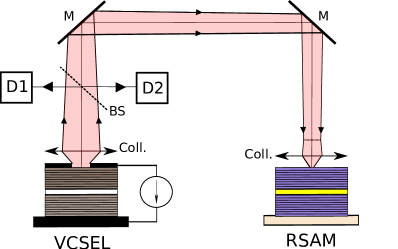
Figure 1: Experimental Set-up: Temperature-stabilized VCSEL and RSAM. Coll.: Aspheric Lens, BS : Beam Splitter, M: Mirror and D1/D2: Detectors and CCD cameras.

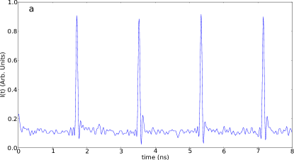
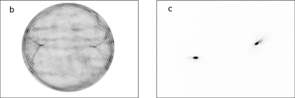
Figure 2: Panel a): Temporal trace of the VCSEL in the mode-locked regime. Panel b): Corresponding Near-Field emission of VCSEL. Panel c): Corresponding Far-field emission from the VCSEL. Intensity grows from white to black. $J$=600 mA.

The set up is shown in Fig. 1. Both the VCSEL and RSAM are mounted on temperature controlled substrates which allow for tuning the resonance frequency of each cavity; parameters are set for having the emission of the VCSEL resonant with the RSAM. The light emitted by the VCSEL is collected by a large numerical aperture (0.68) aspheric lens and a similar lens is placed in front of the RSAM. A $10\,\%$ reflection beam splitter allows for light extraction from the external cavity and to monitor both the VCSEL and the RSAM outputs. Intensity output is monitored by a $33\,$GHz oscilloscope coupled with fast $10\,$GHz detector. Part of the light is sent to two CCD cameras; the first one records the near-field profile of the VCSEL, while the second records the VCSEL’s far-field profile. The light reflected by the RSAM is also used for monitoring and a third CCD camera records the light on the RSAM surface. The external cavity length is fixed to $L=30\,$cm. One of the most important parameters for achieving mode-locking in this setup is the imaging condition of the VCSEL onto the RSAM. We obtain mode-locking when the RSAM is placed in the plane where the exact Fourier transform of the VCSEL near-field occurs. This working condition is obtained by imaging the VCSEL near-field profile onto the front focal plane of the aspheric lens placed in front of the RSAM, while the RSAM is placed onto the back focal plane of this lens. We remark that this leads to a non-local feedback from the RSAM onto the VCSEL: if the RSAM were a normal mirror, the VCSEL near-field profile would be inversely imaged onto itself after a cavity round-trip.

Panel a) in Fig. 2 displays the time trace of the VCSEL in the mode-locking regime which consists of a regular train of pulses with a period equal to the round-trip time in the external cavity $\tau_{e}=2L/c=2\,$ns. The pulse width cannot be determined from the oscilloscope traces, which are limited by our real-time detection system ($10\,$GHz effective bandwidth). However, an estimate of the pulse width can be obtained from the optical spectrum of the output, which exhibits a broad spectral peak whose FWHM is around $0.12\,$nm that corresponds, assuming a time-bandwidth product of $0.4$, to a pulse width of $10\,$ps FWHM. The pulse was also detected by a 42 GHz detector, which confirms a pulse width of less than $12\,$ps FWHM considering the oscilloscope bandwidth limit.

Panels b) and c) in Fig. 2 show the time-averaged near-field and far-field profiles of the VCSEL, respectively. In addition, we verified that the image of the RSAM surface (not shown) is very similar to Fig. 2c), thus revealing that the RSAM is effectively placed in the Fourier plane of the VCSEL’s near-field. The far-field of the VCSEL exhibits two bright, off-axis spots that indicate the presence of two counter-propagating tilted waves along the cross section of the VCSEL. The transverse wave vector of each of these waves is related in direction and modulus to the position of the spots, and their symmetry with respect to the optical axis indicates that the two transverse wave vectors are one opposite to the other.

Figure 3: Temporal signal obtained when detecting simultaneously the two spots (panel a) of the far-field emission of the VCSEL or a single spot (panel b). The insets represent the detected spots in the far-field.

Remarkably, however, no interference pattern is visible in the near-field emission of the VCSEL. The concentric rings close to the limit of the VCSEL arise from current crowding [17] and do not contribute significantly to the bright spots in the far-field, as it was verified by filtering them out. The lack of interference pattern between the counter-propagating waves in the time-averaged near field implies that these waves are not simultaneously present; they rather should alternate each other in time. This is apparent in Fig. 3, where the time trace obtained from the whole far-field is compared to the one obtained by detecting only one of the two bright spots. While the former trace has the characteristics discussed above, the latter trace consists of a periodic train of pulses at a period $2\tau_{e}$. Thus the trace from the whole far-field is obtained by interleaving two identical pulse trains of period $2\tau_{e}$ with a time delay $\tau_{e}$ one with respect to the other, each train corresponding to a tilted wave with opposite transverse wave vector.

This mode-locked dynamics does not depend critically on the transverse wave vector value selected by the system. Such value can be modified by shifting the RSAM device laterally (i.e. along the back focal plane of its collimating lens) or slightly displacing the collimating lens off the axis defined by the centers of the VCSEL and the RSAM. The change in selected transverse wave vector is evidenced by the variations in the separation between the two spots on the RSAM mirror, as shown in Fig. 4. The position of each spot on the RSAM with respect to the optical axis is related to the transverse wave vector $\vec{K}_{\bot}=\vec{K}-\vec{K}_{0}$ of the plane wave by

$$\vec{r}_{s}=\lambda f\frac{\vec{K}_{\bot}}{2\pi}\;,$$

where $f$ is the focal length of the lens in front of the RSAM, $\lambda$ is the wavelength of the light, $\vec{K}$ is the wave vector emitted by the VCSEL while $\vec{K}_{0}$ is its component along the cavity axis. Although substantial changes in emission wavelength —over 4 nm tuning— can be induced in this way, it is observed that within a wide parameter range, the temporal characteristics of the pulse train do not change. This fact opens very interesting possibilities in terms of wavelength tuning and of beam stirring of a mode-locked emission. The only noticeable effect of varying the position of the spot is a slight reduction of the pulse peak power. We attribute this effect to the increased losses experienced in the external cavity by wave vectors with large $K_{\bot}$ as a result of the DBRs reflectivity angular dependence and/or the finite numerical aperture of the collimating lenses. This point will be further discussed in the theoretical section.

Beyond the maximal separation of the two spots on the RSAM shown in Fig. 4, mode-locking is suddenly lost. Importantly, mode-locking strongly deteriorates in regularity when the two spots are brought to coincide, leading, in some cases, to CW emission. Hence, in our setup, regular mode-locking was not achieved with $K_{\perp}\simeq 0$, i.e. for a plane-wave emission almost parallel to the optical axis of the VCSEL.

The mode-locking regime is stable in a very broad range of the VCSEL current, namely $285\,$mA$<J<703\,$mA. If the bias current is varied within this range while keeping the alignment, the separation of the two bright spots in the far-field profile remains constant, see Fig. 5. However the spectral peak corresponding to the mode-locking emission redshifts from 976 nm ($J=285\,$mA) up to 978 nm ($J=703\,$mA) due to Joule heating of the VCSEL. Therefore, the selection of $K_{\bot}$ does not depend on the detuning between the two cavities, at least in the range spanned.

We also found that, for the external cavity length considered, the PML regime is bistable with the off solution for $J<J_{st}$, see [18] for details. In these conditions and after setting the system in the off solution, we were able to start PML emission by perturbing optically the RSAM section at the point where one of the two spots appears when the system operates in the PML regime. The local perturbation has been realized by injecting an external coherent beam tuned with the RSAM cavity resonance and having a waist diameter of less than $10\,\mu$m.

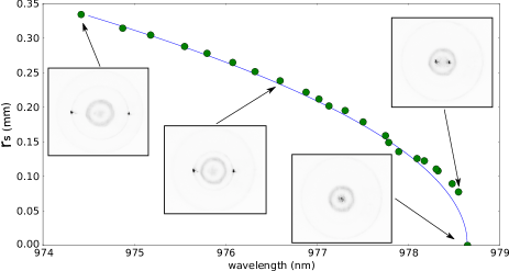
Figure 4: Off-axis position of a single spot in the far-field profile as a function of the spectral emission peak of the VCSEL. Far-field profile is shown for a discrete number of points in the graph. VCSEL emission is in the mode-locking regime for all green points of the graph while the one at the highest wavelength, where a single on-axis spot appears in the far-field profile, corresponds to an irregular dynamics. VCSEL is biased at 700 mA. The transverse wave vector is selected by laterally shifting the RSAM along the back focal plane of its collimating lens. The large size of the RSAM section ( $4\times 4\,$mm) with respect to the far-field size (0.7 mm at most) renders this operation feasible. The blue line has been obtained plotting $r_{s}=\frac{\lambda_{0}f}{2\pi}\sqrt{\lambda^{-2}-\lambda_{0}^{-2}}$, with $\lambda_{0}=978.65\,$nm and $f=8\,$mm. A similar tuning curve is obtained by laterally shifting the collimating lens of the RSAM.

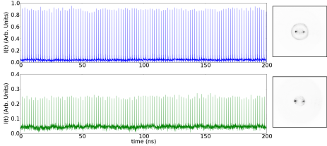
Figure 5: VCSEL time traces emission and corresponding far-field emission profile in the mode-locking regime for two values of the VCSEL bias. The upper and the lower panels correspond to $J=703\,$mA and $J=285\,$mA.

III Discussion of the experimental evidences

These observations disclose a possible explanation about the emergence of the mode-locking regime in our system. From the dynamical point of view, mode-locking is favored when the saturable absorber is more easily saturated than the amplifier [2]. In our scheme, this is achieved when the VCSEL emits a tilted plane wave, which imposes a low power density (hence low saturation) in the gain section and, at the same time, a strong local saturation of the RSAM. The reason is that the VCSEL and the RSAM lie one into the Fourier plane of the other and in these conditions any plane wave emitted by the VCSEL yields a spot on the RSAM and vice-versa. On the other hand, the unsaturated reflectivity of the RSAM is very low ($\sim 1\,\%$) at resonance, rising up to $\sim 60\,\%$ when fully saturated. Hence, if the VCSEL emits a pulse in the form of a plane wave with a transverse wave vector $\vec{K}_{\bot}$, all the power will concentrate on a single spot at $\vec{r}_{s}$ on the RSAM, hereby strongly saturating the RSAM which becomes reflective. The light thus comes back to the VCSEL, where it arrives with a transverse component $-\vec{K}_{\bot}$. Upon amplification and reflection at the VCSEL, the process repeats for this plane wave with opposite transverse wave vector, which is now imaged onto the RSAM at $-\vec{r}_{s}$. Thus, after two round-trips the original wave at $\vec{K}_{\bot}$ overlaps with itself, leading to a pulse train at twice the round-trip time for this wave which is alternating in time with a delay of one round-trip with its replica at $-\vec{K}_{\bot}$.

This explains the observed dynamics, and also the lack of interference pattern in the form of rolls in the VCSEL near-field: even if two tilted waves are propagating within the VCSEL resonator, they alternate in time with a delay of one round-trip in the external cavity, so that they never coexist and do not yield the expected interference pattern. The two spots appearing simultaneously in the far-field (i.e. over the RSAM) are only an artifact of the time-averaging operated by the CCD camera. At variance with tilted waves leading to narrow spots onto the RSAM, the flower mode present on the external frontier of the VCSEL does not contribute to PML. In fact, the Fourier Transform of such flower mode is a radial Bessel function of large order $\sim J_{m}\left(r\right)$ with $m\gg 1$, which corresponds to an extended ring profile. In this case, the power density on the RSAM remains always below the saturation fluence of the RSAM.

While the above scenario is valid for a large interval of values of the transverse wave vector $\vec{K}_{\bot}$, experimental results show that the system selects a well-defined value when operating in the PML regime. In principle, this selection may arise from several factors. On the one hand, both the VCSEL and the RSAM are Fabry-Perot cavities defined by Bragg mirrors which complex reflectivity have an angular dependence. Moreover, the reflectivity of a Fabry-Perot cavity depends not only on the wavelength but also on the angle of incidence of the light, and the resonant wavelength of the cavity blue-shifts as the incidence angle increases. This effect can be further enhanced in our system due to the compound-cavity effect. Nevertheless, experimental evidences shown in Fig. 5, where the VCSEL cavity resonance is varied over 2 nm while leaving the transverse wave vector unchanged, seems to indicate that cavities detuning do not play an important role in selecting the value of $\vec{K}_{\bot}.$ This can be understood when considering that the FWHM bandwidth of the RSAM absorption curve (16 nm) is much larger than the VCSEL one (1 nm).

On the other hand, wave vector selectivity may also arise from any imperfections on the RSAM/VCSEL mirrors that break the spatial invariance. State-of-the-art fabrication process does not fully prevent from formation of small size (a few $\mu$m) defects in the transverse plane of semiconductor micro-resonators. These are in general local spatial variations of the semiconductor resonator characteristics [19], which in the case of RSAM would be mainly related to a local variation of unsaturated reflectivity. Visual inspection of the reflection profile of a transversally homogeneous injected monochromatic field onto several used RSAMs has indeed shown the existence of these local variations. Such inhomogeneities on the RSAM surface may correspond to locations where the RSAM exhibits a lower unsaturated reflectivity, hence leading the system to select the tilted wave which image on the RSAM surface coincide with one of these defect. By laterally shifting the RSAM along the back focal plane of its collimating lens, the position of the defect changes in the far-field plane, thus selecting a tilted wave with another transverse wave vector component. This leads to a continuous scan of the distance between the two spots in the far-field, as shown in Fig. 4 and a corresponding change of the emission wavelength, as expected for tilted waves. The experimental evidence of Fig. 4 seems to indicate that, in our system, the presence of these inhomogeneities is ruling the selection of the transverse wave vector. The role of small imperfections in the RSAM structure in the transverse wave vector selection is confirmed by the theoretical results in the next section.

IV Theoretical results

Our model for the dynamical evolution of the fields $E_{j}$ and the normalized carrier density $N_{j}$ in the quantum well (QW) regions of the VCSEL $(j=1)$ and the RSAM $(j=2)$ is deduced in detail in the appendix, and it reads

$$\dot{E}_{1} \negthickspace\negthickspace=\negthickspace\negthickspace \left[\left(1-i\alpha_{1}\right)N_{1}-1+i\Delta_{\perp}+c_{1}\Delta_{\perp}^{2}\right]E_{1}+h_{1}Y_{1},$$ (1)

$$\dot{E}_{2} \negthickspace\negthickspace=\negthickspace\negthickspace \left[\left(1-i\alpha_{2}\right)N_{2}-z+ib\Delta_{\perp}+c_{2}\Delta_{\perp}^{2}\right]E_{2}+h_{2}Y_{2},$$ (2)

$$\dot{N}_{1} \negthickspace\negthickspace=\negthickspace\negthickspace \gamma_{1}\left[J_{1}-\left(1+|E_{1}|^{2}\right)N_{1}\right]+\mathcal{D}_{1}\Delta_{\perp}N_{1},$$ (3)

$$\dot{N}_{2} \negthickspace\negthickspace=\negthickspace\negthickspace \gamma_{2}\left[J_{2}-\left(1+s|E_{2}|^{2}\right)N_{2}\right]+\mathcal{D}_{2}\Delta_{\perp}N_{2},$$ (4)

where $\Delta_{\perp}=\partial_{x}^{2}+\partial_{y}^{2}$ is the transverse Laplacian and $Y_{j}$ denotes the field injected in device $j$. In Eqs. (1-4) time and space are normalized to the photon lifetime $\kappa_{1}^{-1}$ and the diffraction length in the VCSEL $L_{d}$, respectively. The complex parameter $z$ is decomposed as $z=a-i\delta$ where $a$ represents the ratio of the photon decay rates between the VCSEL and the RSAM cavities and $\delta$ is the scaled detuning between the two cavity resonances. The scaled carrier recovery rates and the biases are denoted $\gamma_{j}$ and $J_{j}$ respectively. We define the ratio of the saturation intensities of the VCSEL and the RSAM as $s$. The angular dependence from the reflectivity of the DBR mirrors as well as the one stemming from the Fabry-Perot cavities are contained in the transverse Laplacian and the parameters $c_{1,2}.$ The RSAM being a broadband fast absorber, it is characterized by $J_{2}<0$, $\gamma_{2}\gg\gamma_{1}$, $a\gg 1$ as well as $s\gg 1$.

IV-1 Injected fields and device coupling

In the case of a self-imaging configuration, the link between the two devices is achieved by expressing the emitted fields $O_{j}$ as a combination of the reflection of the injection fields $Y_{j}$ and the self-emission $E_{j}$, which reads

$$O_{j}\left(r,t\right)=\eta_{j}E_{j}\left(r,t\right)-Y_{j}\left(r,t\right),$$ (5)

where we defined $\eta_{j}=t_{1}^{j}/\left(1+r_{1}^{j}\right)$ with $t_{1}^{j}$ and $r_{1}^{j}$ the transmission and reflection coefficients in amplitude of the emitting DBR from the inside to the outside of the cavity. Considering the propagation delay and the losses incurred by the beam-splitter allowing for the light extraction, the link between the two devices in ensured by the following two delayed Algebraic Equations [20]

$$Y_{1}\left(r,t\right)=t_{bs}O_{2}\left(r,t-\tau_{e}\right),Y_{2}\left(r,t\right)=t_{bs}O_{1}\left(r,t-\tau_{e}\right),$$ (6)

with $t_{bs}$ a complex number whose modulus and phase model the losses induced by the beam-splitter and the single trip feedback phase, respectively.

However, the image of the VCSEL through its collimator is placed exactly at the object focal plane of the collimator in front of the RSAM. In turn, the RSAM is on the image focal plane of its collimator. In this configuration, and assuming that the collimators have a large diameter, the field injected in one device is the (delayed) Fourier transform in space of the field coming from the other, which is modelized via Kirchhoff’s formula for a lens with focal length $f$ as

$$Y_{1}(r,t) \negthickspace\negthickspace=\negthickspace\negthickspace t_{bs}\int\,O_{2}(r^{{}^{\prime}},t-\tau_{e})e^{-i\frac{\omega_{0}}{c}\frac{r\text{$\cdot$r'}}{f}}d^{2}r^{\prime}\equiv\mathcal{F}_{\tau}(O_{2})$$ (7)

$$Y_{2}(r,t) \negthickspace\negthickspace=\negthickspace\negthickspace t_{bs}\int\,O_{1}(r^{{}^{\prime}},t-\tau_{e})e^{-i\frac{\omega_{0}}{c}\frac{r\text{$\cdot$r'}}{f}}d^{2}r^{\prime}\equiv\mathcal{F}_{\tau}(O_{1})$$ (8)

and where the beam-splitter losses may contain a normalization constant due to the Kirchhoff’s integral. It is worth remarking that Eqs. (7-8) describe the coupling of the two devices to all orders of reflection in the external cavity. They define a delayed map where the field injected into one device returns inverted. This can be seen, for instance, using Eq. (5) and saying that the RSAM has an effective reflectivity such that $O_{j}=r_{eff}Y_{j}$ and substituting in Eq. (7), which yields

$$Y_{1}(r_{\perp},t)=\mu E_{1}(-r_{\perp},t-2\tau)$$ (9)

where we have used that $\mathcal{F}_{\tau}\circ\mathcal{F}_{\tau}\left[Y_{2}\right]=\alpha Y_{2}\left(-r_{\perp},t-2\tau\right)$ and $\mu$ = t${}_{bs}^{2}r_{eff}$ describes the combined effect of the beam splitter and of the RSAM reflection. Thus, after one round-trip, $Y_{1}$ overlaps with a spatially reversed copy of itself, and it requires a second round-trip to achieve proper overlap.

IV-2 Parameters

The reflectivities of the DBRs in the VCSEL and the RSAM are taken as $\left(r_{1}^{\left(1\right)},r_{2}^{\left(1\right)}\right)=\left(\sqrt{0.942},1\right)$ and $\left(r_{1}^{\left(2\right)},r_{2}^{\left(2\right)}\right)=\left(\sqrt{0.59},1\right)$. We assume that the single trip in the VCSEL and the RSAM is $\tau=30\,$fs corresponding to an effective length $L_{z}=2.6\,\mu$m with a index of $n=3.5$. This gives us $\kappa_{1}=10^{12}\,$rad.s^-1 and $\kappa_{2}=10^{13}\,$rad.s^-1, yielding a FWHM for the resonances of $\Delta\lambda_{j}=\kappa_{j}\lambda_{0}^{2}/\left(\pi c\right)$ of $1\,$nm and $10\,$nm respectively. Incidentally, we find that $a=10$ and $\left(h_{1},h_{2}\right)=\left(2,20\right)$. The diffraction length is found to be $L_{d}=\sqrt{L_{z}\left[q_{0}\left(1-r_{1}r_{2}\right)\right]^{-1}}=2\,\mu$m. We define two numerical domains which are twice the size of the VCSEL and of the RSAM which have both a normalized length $L_{\perp}=200$. The other parameters are $\alpha_{1}=2$, $\alpha_{2}=0.5$, $b=10^{-2}$,$\gamma_{1}=10^{-3}$, $\gamma_{2}=0.1$, $s=10$, $t_{bs}=0.9$, $\mathcal{D}_{1}=\mathcal{D}_{2}=10^{-3}$ $c_{1}=10^{-2}$ and $c_{2}=10^{-6}.$

IV-3 Numerical considerations

The simulation of PML lasers is a very demanding problem from the computational point of view: while pulses may form on a relatively short time scale of a few tens of round-trips, the pulse characteristics only settle on a much longer time scale [21]. If anything, the complex transverse dynamics present in our case shall slow down the dynamics even further. Considering a delay of $\tau_{e}=2\,$ns and a time step of $\delta t=10^{-2}$ implies that one must keep four memory buffers for $E_{j}$ and $Y_{j}$ of size $\left(\tau_{e}\kappa_{1}/\delta t\right)N_{x}N_{y}\sim 2\times 10^{3}N_{x}N_{y}$ with $N_{x}$ and $N_{y}$ the number of mesh points in the two transverse directions. This amounts to $32\,$Gigabytes with $N_{x}=N_{y}=512$. Notice in addition that such values of $N_{x,y}$ are not particularly large if one considers that only half of the mesh discretization in the VCSEL is electrically pumped, the rest being used only for letting the field decay to zero and prevent aliasing, a common problem with spectral methods in broad-area lasers, see for instance [22] for a discussion. The time step of $\delta t=10^{-2}$ is neither particularly small if one considers the stiffness incurred by the RSAM response. For these reasons we restrict our analysis to a single transverse dimension. We believe that the main spatial feature being lost by such simplification is the description of the non mode-locked two dimensional radial flower mode [17] on the border of the VCSEL, which has already been qualitatively discussed. To conclude, for the sake of simplicity, we used a time delay of $\tau_{e}=200\,$ps (instead of $1\,$ns) to avoid the temporal complexity of our setup (leading to localized structures, as discussed in [18]), and to concentrate only on the spatial aspects of the problem. We integrated numerically Eqs. (1-4) using a semi-implicit split-step method where the spatial operators are integrated using the Fourier Transform. Such semi-implicit method is particularly appropriate to the stiffness induced by the broad response of the RSAM. The simulation time was $500$ single-trips in the external cavity, i.e. $100\,$ns.

IV-4 RSAM characteristics

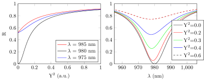
Figure 6: Reflectivity as a function of the input field intensity (left) for various values of the wavelength, the resonance being chosen to be $\lambda_{0}=980\,$nm and (right) reflectivity as a function of wavelength for increasing input power.

The basic properties of the RSAM can be found assuming an incoming plane wave of amplitude $Y$ at normal incidence and at frequency $\omega$ i.e. $Y_{2}=Y\exp\left(-i\omega t\right)$. The response of the RSAM is given by

$$\left(z-i\omega-\frac{J_{2}\left(1-i\alpha_{2}\right)}{1+s|E_{2}|^{2}}\right)E_{2} = h_{2}Y.$$ (10)

The effective reflectivities are obtained setting $O_{2}=rY_{2}$ that is to say $r=E_{2}/Y_{2}-1$ yielding the unsaturated and saturated responses as

$$r_{u}=\frac{h_{2}-z+i\omega+J_{2}\left(1-i\alpha_{2}\right)}{z-i\omega-J_{2}\left(1-i\alpha_{2}\right)},r_{s}=\frac{h_{2}-z+i\omega}{z-i\omega}.$$ (11)

By choosing $J_{2}=a-h_{2}$ we obtain a perfectly absorbing RSAM, i.e. $r_{u}=0$ at the frequency $\omega=\delta+\alpha\left(a-h_{2}\right)$. In between these unsaturated and saturated regimes, the effective reflectivity can be obtained by solving Eq. (10) numerically. We represent the results of this procedure for $R=\left|r\right|^{2}$ in Fig. 6.

IV-5 Defect in the RSAM surface

We assume that the impurity on the RSAM surface has the effect of locally lowering the reflectivity of the top mirror. As such the parameters $a$ and $h_{2}$ are allowed to vary in the transverse dimension. A decrease of $r_{1}^{\left(2\right)}$of $0.1$ modifies $a$ and $h_{2}$ to be $a=12$ and $h_{2}=24$. We assume a Gaussian profile for such transverse variations whose FWHM is $\sim 5\,\mu$m.

IV-A Mode-Locking dynamics

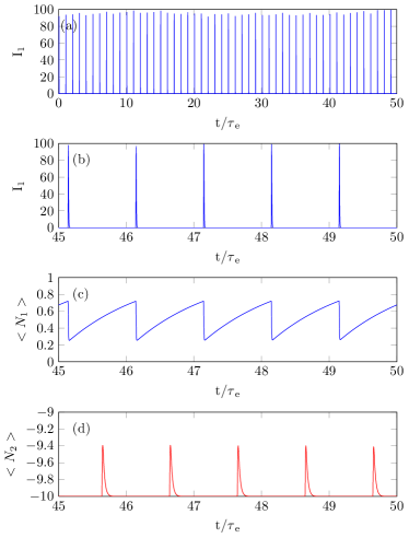
Figure 7: Panels a) and b): Averaged Intensity profile $I_{1}$ as a function of time showing stable PML. Panels c) and d) represent the averaged population inversion in the VCSEL and in the RSAM as a function of time.

The bias current is fixed to $J_{1}=0.92$, i.e. below the threshold of the solitary VCSEL but above the threshold of the compound device. We depict in Fig. 7, the output time trace for the intensity averaged over the surface of the VCSEL as well as the averaged population inversion in the active region of the VCSEL and in the RSAM. One recognizes the standard PML temporal pattern where the gain experiences depletion during the passing of the pulse followed by an exponential recovery. The same yet inverted pattern is also visible on the RSAM population inversion. We found the pulse width to be of the order of $4\,$ps, in good qualitative agreement with the experimental results.

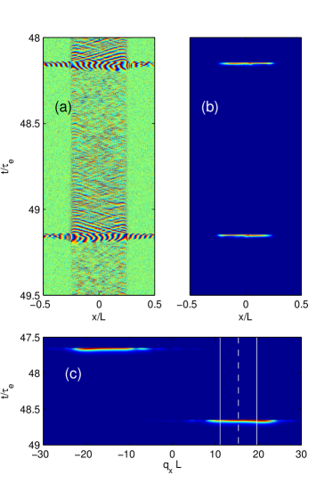
Figure 8: Panel a): Phase profile of $E_{1}$ as a function of space and time. A tilted wave with alternate wave vector from one round-trip to the next is clearly visible. Panel b) Intensity profile of $E_{1}$ showing that the transverse intensity profile is uniform. Panel c): Population inversion in the RSAM. The FWHM size of the population inversion spot is $\sim 6\,\mu$m and the RSAM is fully saturated locally by the pulse.

Such averaged representation describes well the experimental situation when the full output of the VCSEL is captured by the photo-detector. Yet it does not shed light onto the hidden transverse dynamics. We represent in Fig. 8 the spatially resolved temporal output of the VCSEL. In Fig. 8a) the phase profile $\phi_{1}=\arg\left(E_{1}\right)$ discloses the existence of alternate transverse waves while the intensity profile in Fig. 8b) remains uniform. Such field profile directly impings the RSAM via its Fourier Transform which explains that the temporal time trace of population inversion in the RSAM (Fig. 8c)) exhibits two spots at two opposite locations with respect to its center. In Fig. 8c) we represented the center of the pinning potential with a dotted line while the two white lines represent its FWHM. The horizontal axis in Fig. 8c) is scaled in normalized spatial frequencies. The transverse value of the wave vector here is $\sim 16$ which corresponds to $8$ transverse oscillations along the active region of the VCSEL, i.e. a wavelength of $\sim 25\,\mu$m.

We found that by slowly displacing the center of the pinning potential it was possible to tune the normalized transverse wave vector between $q_{x}L=0$ and $q_{x}L=36$, which corresponds to a minimal wavelength of $11\,\mu$m. The associated shift in the emission wavelength is $\sim 4\,$nm around $980\,$nm, in excellent agreement with the experimental results. Several points along such tuning curve are presented in Fig. 9. All cases correspond to stable PML regimes that would seem to be almost identical if one would considers only the averaged temporal output like e.g. in Fig. 7. Noteworthy, we also found some perfectly regular PML regimes when the inhomogeneity was located at the center of the RSAM. We provide several explanations for such discrepancy. First, the dissipation of the energy and of the associated heat incurred by the light absorption is doubled when the two spots are well separated onto the RSAM. Such thermal effects are not taken in consideration by our model. Second, other spatial inhomogeneities, these ones detrimental to PML, could very well be located on the sides of the pinning defect favoring PML. When the two spots become less and less separated experimentally, the spot that is not experiencing the pinning defect (i.e. the left spot in Fig. 9) will eventually be the victim of such other detrimental inhomogeneities.

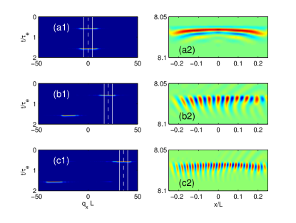
Figure 9: Evolution of the transverse wave vector as a function of the position of the pinning potential. Panels a1), b1) and c1) correspond to the population inversion in the RSAM while the panels a2), b2) and c2) correspond to the real part of $E_{1}$. The FWHM size of the population inversion spot in the RSAM corresponds to $\sim 6\,\mu$m and the RSAM is fully saturated locally by the pulse.

V Conclusions

We have shown that electrically biased broad-area VCSELs with optical feedback from a RSAM can be passively mode-locked when the VCSEL and RSAM are placed each at the Fourier plane of the other. In this configuration, the system emits a train of pulses of $\sim 10\,$ps width with a period equal to the round-trip time of the external cavity $\tau_{e}$. In this PML regime the time-averaged VCSEL far-field, which is imaged onto RSAM plane, exhibits two bright peaks symmetrically located around the optical axis, thus indicating that the VCSEL emits two tilted waves with opposite transverse components. The time traces corresponding to each spot consist of a pulse train with a period $2\tau_{e}$, and the two trains are delayed by one round-trip one with respect to the other. Accordingly, the two tilted waves are alternatively emitted at every round-trip. We have shown that the mechanism leading to wave vector selection is related to the existence of inhomogeneities in the transverse section of the RSAM. Because the RSAM is in the Fourier plane of the VCSEL near-field, a defect may favor a tilted wave emission with a well-defined transverse component. By shifting the RSAM laterally, the defect moves in the Fourier plane, thus selecting another transverse wave vector and allowing for wavelength tuning of the mode-locked emission.

VI Appendix

Our approach extends the methodology developed in [23] for single-mode VCSELs under optical injection to the case of broad-area devices. The Quantum-Well active region is considered as infinitely thin, and the wave equation is exactly solved inside the cavity for monochromatic plane-waves. Transforming back to a spatio-temporal representation provides the time-domain evolution of the field inside cavity. Finally, the coupling of the two cavities is included by describing how the injection terms depend on the intra-cavity fields.

The starting point is the scalar Maxwell equation for a monochromatic field as in [23]

$$\left(\partial_{z}^{2}+\Delta_{\perp}\right)\mathcal{E}\left(\omega,\vec{r}\right)+\frac{\omega^{2}}{\upsilon^{2}}\mathcal{E}\left(\omega,\vec{r}\right) \negthickspace\negthickspace=\negthickspace\negthickspace \frac{-\omega^{2}}{c^{2}\varepsilon_{0}}\mathcal{P}\left(\omega,\vec{r}\right)\,,$$ (12)

where $\Delta_{\perp}=\partial_{x}^{2}+\partial_{y}^{2}$, $\mathcal{P}$ is the polarization of the QW active region and $\upsilon=c/n$ with $n$ the index of refraction. In the longitudinal direction, the cavity is defined by two Bragg mirrors at $z=0$ and $z=L$.

Fourier transforming over the transverse coordinates yields

$$\left(\partial_{z}^{2}+\frac{\omega^{2}}{\upsilon^{2}}-q_{\perp}^{2}\right)\mathcal{E}\left(\omega,q_{\perp},z\right) \negthickspace\negthickspace\negthickspace=\negthickspace\negthickspace\negthickspace \frac{-\omega^{2}W}{c^{2}\varepsilon_{0}}P\left(\omega,q_{\perp}\right)\delta_{l}.$$ (13)

We assumed that the Quantum Well(s) of width $W\ll\lambda$ are located at $z=l$ and defined $\delta_{l}=\delta\left(z-l\right)$. In the empty regions where there is no polarization the solution of Eq. (13) reads

$$\mathcal{E}\left(\omega,q_{\perp},z\right)=\begin{cases}L_{+}e^{iQz}+L_{-}e^{-iQz}&\mbox{if }0<z<l\\ R_{+}e^{iQz}+R_{-}e^{-iQz}&\mbox{if }l<z<L\end{cases}$$ (14)

where the longitudinal wave vector $Q\left(q_{\perp},\omega\right)=\sqrt{\frac{\omega^{2}}{\upsilon^{2}}-q_{\perp}^{2}}$ . The boundary conditions at the mirrors and at the QW impose that

$$r_{1}L_{-}+t_{1}^{{}^{\prime}}Y = L_{+}$$ (15)

$$r_{2}R_{+}e^{iQL} = R_{-}e^{-iQL}$$ (16)

$$L\left(l\right) = R\left(l\right)=\mathcal{E}\left(\omega,q_{\perp},l\right)$$ (17)

$$\partial_{z}R\left(l\right)-\partial_{z}L\left(l\right) = -\frac{\omega^{2}}{\varepsilon_{0}c^{2}}P$$ (18)

where the primed indexes are for transmission and reflection processes starting outside of the cavity, $r_{1}$ and $r_{2}$ the top (emitting) and bottom reflectivities and $Y$ is the amplitude of the external field impinging on the device. After some algebra the equation linking $\mathcal{E}$, $P$ and $Y$ is found to be

$$F_{1}\left(Q\right)\mathcal{E} = -\frac{\omega^{2}}{2iQ\varepsilon_{0}c^{2}}\Gamma WP+F_{2}\left(Q\right)Y$$ (19)

with

$$F_{1}=\left(1-r_{1}r_{2}e^{2iQL}\right),\,F_{2}=t^{\prime}_{1}e^{iQl}\left(1+r_{2}e^{2iQ\left(L-l\right)}\right).$$ (20)

The modes of the VCSEL correspond to the minima of $F_{1}$, and the QW is placed in order to maximize the optical confinement factor $\Gamma=\left(1+r_{1}e^{2iQl}\right)\left(1+r_{2}e^{2iQ\left(L-l\right)}\right)$ for the fundamental mode at $q_{\perp}=0$. For fixed magnitude of the reflectivities, this is achieved by imposing that

$$2\frac{\omega}{\upsilon}l+\phi_{1}=2\pi n_{1},\,2\frac{\omega}{\upsilon}(L-l)+\phi_{2}=2\pi n_{2}$$

where $\phi_{1,2}$ are the phases of the reflectivities $r_{1,2}$ and $n_{1}$and $n_{2}$ two integers. Thus the modal frequencies are determined by the effective cavity length $L_{e}=L+2\upsilon\left(\phi_{1}+\phi_{2}\right)/\omega$. Around any modal frequency $\omega_{0}$, and in paraxial conditions, $F_{2}$ and $\Gamma/Q$ vary much more slowly than $F_{1}$. In order to have a spatio-temporal description of the dynamics of the field, we then fix $\Gamma/Q$ and $F_{2}$ and expand

$$F_{1}=F_{1}^{0}+(\omega-\omega_{0})\partial_{\omega}F_{1}+q_{\perp}^{2}\partial_{q_{\perp}^{2}}F_{1}+\cdots$$ (21)

and transform back to space and time using that $\omega\rightarrow\omega_{0}+i\partial_{t}$ and $q_{\perp}^{2}\rightarrow-\Delta_{\perp}$. Since $F_{1}$ is at a minimum of its modulus, $\partial_{\omega}F_{1}$ is purely imaginary, and the field evolution can be written as

$$\tau_{c}\frac{d\mathcal{E}}{dt} = i\frac{\omega_{0}\Gamma W}{2n\varepsilon_{0}c}P-\kappa\tau_{c}\mathcal{E}+iL_{diff}^{2}\Delta_{\perp}\mathcal{E}$$ (22)

$$+ t_{1}^{{}^{\prime}}(1+|r_{2}|)\left(-1\right)^{m}Y+C\Delta_{\perp}^{2}\mathcal{E}$$

where $\tau_{c}\approx|r_{1}r_{2}|2L_{e}/v$ is the effective cavity transit time, $\kappa\approx 1-|r_{1}r_{2}|$ are the cavity losses under normal incidence at resonance, $L_{diff}\approx|r_{1}r_{2}|\frac{2\upsilon\partial_{q_{\perp}^{2}}L_{e}}{\omega_{0}}$ is the diffraction length, and $C$ describes the variation of cavity losses with the angle of incidence.

The polarization of the QW active region determines the gain and index change induced by the carriers, and we adopt the simple adiabatic approximation

$$P=\varepsilon_{0}(\alpha-i)g_{0}(N-N_{t})E$$ (23)

where $\alpha$ is Henry’s linewidth enhancement factor, $g_{0}$ is the material gain coefficient and $N_{t}$ is the transparency carrier density. The carrier density, in turn, obeys the standard description as in [23]. Upon normalization, the evolution for the field and carrier density can be written as

$$\frac{\partial E}{\partial t} = \left[\left(1-i\alpha\right)N-1+i\Delta_{\perp}+c\Delta_{\perp}^{2}\right]E+hY,$$ (24)

$$\frac{\partial N}{\partial t} = \gamma\left[J-\left(1+|E|^{2}\right)N\right]+\mathcal{D}\Delta_{\perp}N,$$ (25)

where $\gamma$ is the scaled carrier lifetime, $J$ is the current injection above transparency, $\mathcal{D}$ is the diffusion coefficient and $h$ describes the coupling of the output field onto the QW and reads

$$h = t_{1}^{{}^{\prime}}\frac{1+r_{2}}{1-r_{1}r_{2}}$$ (26)

As a last step, we evaluate the field at the laser output $O$ as a combination of the reflection of the injected beam $r_{1}^{{}^{\prime}}Y$ as well as transmission of the left intra-cavity propagating field $L_{-}$, i.e. $O=t_{1}L_{-}+r_{1}^{{}^{\prime}}Y$. Around resonance and using the Stokes relations $tt^{\prime}-rr^{\prime}=1$ and $r^{\prime}=-r$ we find, defining $\eta=t_{1}/\left(1+r_{1}\right)$

$$O = \eta\left(-1\right)^{m}\mathcal{E}-Y$$ (27)

although the $\left(-1\right)^{m}$ is irrelevant in the sense that the QW experiences also a field with a $\left(-1\right)^{m}$ which can therefore be removed. In the case of two devices, we scale the photon lifetime, the coupling and the saturation field with respect to the first one leading to the following definitions

$$h_{2}=t_{3}^{{}^{\prime}}\frac{1+r_{4}}{1-r_{1}r_{2}}\frac{r_{1}r_{2}}{r_{3}r_{4}}\>,\>a=\frac{1-r_{3}r_{4}}{1-r_{1}r_{2}}\frac{r_{1}r_{2}}{r_{3}r_{4}}\>,\>b=\frac{r_{1}r_{2}}{r_{3}r_{4}}$$ (28)

and $s=\left(g_{2}\gamma_{1}\right)/\left(g_{1}\gamma_{2}\right)$.

Mathias Marconi was born in Nice, France, in 1988. From 2006 to 2011, he was a student at Universit de Nice Sophia Antipolis (UNS), France. In 2011, he was an exchange student at Strathclyde university, Glasgow, U.K. The same year he obtained the Master degree in optics from UNS. He is currently pursuing the Ph.D. degree at the Institut Non-lin aire de Nice, Valbonne, France. His research interests include semiconductor laser dynamics and pattern formation in out of equilibrium systems. He is a member of the European Physical Society.

Julien Javaloyes (M’11) was born in Antibes, France in 1977. He obtained his M.Sc. in Physics at the ENS Lyon the PhD in Physics at the Institut Non Lin aire de Nice / Universit de Nice Sophia-Antipolis working on recoil induced instabilities and self-organization processes in cold atoms. He worked on delay induced dynamics in coupled semiconductor lasers, VCSEL polarization dynamics and monolithic mode-locked semiconductor lasers. He joined in 2010 the Physics Department of the Universitat de les Illes Balears as a Ram n y Cajal fellow. His research interests include laser dynamics and bifurcation analysis.

Salvador Balle (M’92) was born in Manacor, Mallorca. He graduated in Physics at the Universitat Aut noma de Barcelona, where he obtained a PhD in Physics on the electronic structure of strongly correlated Fermi liquids. After postdoctoral stages in Palma de Mallorca and Philadelphia where he became interested in stochastic processes and Laser dynamics, he joined in 1994 the Physics Department of the Universitat de les Illes Balears, where he is Professor of Optics since 2006. His research interests include laser dynamics, semiconductor optical response modeling, multiple phase fluid dynamics and laser ablation.

Massimo Giudici (M’09) received the "Laurea in Fisica" from University of Milan in 1995 and Ph.D from Universit de Nice Sophia-Antipolis in 1999. He is now full professor at Universit de Nice Sophia-Antipolis and deputy director of the laboratory “Institut Non Lin aire de Nice”, where he carries out his research activity. Prof. Giudici’s research interests revolve around the spatio-temporal dynamics of semiconductor lasers. In particular, he is actively working in the field of dissipative solitons in these lasers. His most important contributions concerned Cavity Solitons in VCSELs, longitudinal modes dynamics, excitability and stochastic resonances in semiconductor lasers and the analysis of lasers with optical feedback. He is authors of more than 50 papers and he is Associated Editor of IEEE Photonics Journal.

References

- [1] A. Gordon and B. Fischer, “Phase transition theory of many-mode ordering and pulse formation in lasers,” Physical Review Letters, vol. 89, pp. 103 901–3, 2002.
- [2] H. A. Haus, “Mode-locking of lasers,” IEEE J. Selected Topics Quantum Electron., vol. 6, pp. 1173–1185, 2000.
- [3] ——, “Theory of mode locking with a fast saturable absorber,” Journal of Applied Physics, vol. 46, pp. 3049–3058, 1975.
- [4] ——, “Theory of mode locking with a slow saturable absorber,” Quantum Electronics, IEEE Journal of, vol. 11, pp. 736–746, 1975.
- [5] H. Dorren, D. Lenstra, Y. Liu, M. Hill, and G.-D. Khoe, “Nonlinear polarization rotation in semiconductor optical amplifiers: theory and application to all-optical flip-flop memories,” Quantum Electronics, IEEE Journal of, vol. 39, no. 1, pp. 141–148, Jan 2003.
- [6] E. P. Ippen, “Principles of passive mode locking,” Appl. Phys. B, vol. 58, pp. 159–170, 1994.
- [7] J. Javaloyes, J. Mulet, and S. Balle, “Passive mode locking of lasers by crossed-polarization gain modulation,” Phys. Rev. Lett., vol. 97, p. 163902, Oct 2006. [Online]. Available: http://link.aps.org/doi/10.1103/PhysRevLett.97.163902
- [8] K. G. Wilcox, Z. Mihoubi, G. J. Daniell, S. Elsmere, A. Quarterman, I. Farrer, D. A. Ritchie, and A. Tropper, “Ultrafast optical stark mode-locked semiconductor laser,” Opt. Lett., vol. 33, no. 23, pp. 2797–2799, 2008.
- [9] R. Fork, C. Shank, R. Yen, and C. Hirlimann, “Femtosecond optical pulses,” Quantum Electronics, IEEE Journal of, vol. 19, no. 4, pp. 500 – 506, apr 1983.
- [10] U. Keller, K. J. Weingarten, F. X. Kärtner, D. Kopf, B. Braun, I. D. Jung, R. Fluck, C. Hönninger, N. Matuschek, and J. Aus der Au, “Semiconductor saturable absorber mirrors (SESAM’s) for femtosecond to nanosecond pulse generation in solid-state lasers,” Selected Topics in Quantum Electronics, IEEE Journal of, vol. 2, pp. 435–453, 1996.
- [11] E. A. Avrutin, J. H. Marsh, and E. L. Portnoi, “Monolithic and multi-GigaHertz mode-locked semiconductor lasers: Constructions, experiments, models and applications,” IEE Proc.-Optoelectron., vol. 147, pp. 251–278, 2000.
- [12] B. Rudin, V. J. Wittwer, D. J. H. C. Maas, M. Hoffmann, O. D. Sieber, Y. Barbarin, M. Golling, T. Südmeyer, and U. Keller, “High-power mixsel: an integrated ultrafast semiconductor laser with 6.4 w average power,” Opt. Express, vol. 18, no. 26, pp. 27 582–27 588, Dec 2010. [Online]. Available: http://www.opticsexpress.org/abstract.cfm?URI=oe-18-26-27582
- [13] K. G. Wilcox, A. C. Tropper, H. E. Beere, D. A. Ritchie, B. Kunert, B. Heinen, and W. Stolz, “4.35 kw peak power femtosecond pulse mode-locked vecsel for supercontinuum generation,” Opt. Express, vol. 21, no. 2, pp. 1599–1605, Jan 2013. [Online]. Available: http://www.opticsexpress.org/abstract.cfm?URI=oe-21-2-1599
- [14] I. Fischer, O. Hess, W. Elsässer, and E. Göbel, “Complex spatio-temporal dynamics in the near-field of a broad-area semiconductor laser,” Europhys. Lett., vol. 35, pp. 579–584, 1996.
- [15] G. H. B. Thompson, “A theory for filamentation in semiconductor lasers including the dependence of dielectric constant on injected carrier density,” Opto-electronics, vol. 4, pp. 257–310, 1972.
- [16] M. Grabherr, R. Jager, M. Miller, C. Thalmaier, J. Herlein, R. Michalzik, and K. Ebeling, “Bottom-emitting vcsel’s for high-cw optical output power,” Photonics Technology Letters, IEEE, vol. 10, no. 8, pp. 1061–1063, Aug 1998.
- [17] I. V. Babushkin, N. A. Loiko, and T. Ackemann, “Eigenmodes and symmetry selection mechanisms in circular large-aperture vertical-cavity surface-emitting lasers,” Phys. Rev. E, vol. 69, p. 066205, Jun 2004. [Online]. Available: http://link.aps.org/doi/10.1103/PhysRevE.69.066205
- [18] M. Marconi, J. Javaloyes, S. Balle, and M. Giudici, “How lasing localized structures evolve out of passive mode locking,” Phys. Rev. Lett., vol. 112, p. 223901, Jun 2014. [Online]. Available: http://link.aps.org/doi/10.1103/PhysRevLett.112.223901
- [19] J. Oudar, R. Kuszelewicz, B. Sfez, J. Michel, and R. Planel, “Prospects for further threshold reduction in bistable microresonators,” Optical and Quantum Electronics, vol. 24, no. 2, pp. S193–S207, 1992. [Online]. Available: http://dx.doi.org/10.1007/BF00625824
- [20] J. Javaloyes and S. Balle, “Multimode dynamics in bidirectional laser cavities by folding space into time delay,” Opt. Express, vol. 20, no. 8, pp. 8496–8502, Apr 2012. [Online]. Available: http://www.opticsexpress.org/abstract.cfm?URI=oe-20-8-8496
- [21] ——, “Mode-locking in semiconductor Fabry-Pérot lasers,” Quantum Electronics, IEEE Journal of, vol. 46, no. 7, pp. 1023 –1030, july 2010.
- [22] A. Perez-Serrano, J. Javaloyes, and S. Balle, “Spectral delay algebraic equation approach to broad area laser diodes,” Selected Topics in Quantum Electronics, IEEE Journal of, vol. PP, no. 99, pp. 1–1, 2013.
- [23] J. Mulet and S. Balle, “Mode locking dynamics in electrically-driven vertical-external-cavity surface-emitting lasers,” Quantum Electronics, IEEE Journal of, vol. 41, no. 9, pp. 1148–1156, 2005.