DC approximation approaches for sparse optimization

Abstract

Sparse optimization refers to an optimization problem involving the zero-norm in objective or constraints. In this paper, nonconvex approximation approaches for sparse optimization have been studied with a unifying point of view in DC (Difference of Convex functions) programming framework. Considering a common DC approximation of the zero-norm including all standard sparse inducing penalty functions, we studied the consistency between global minimums (resp. local minimums) of approximate and original problems. We showed that, in several cases, some global minimizers (resp. local minimizers) of the approximate problem are also those of the original problem. Using exact penalty techniques in DC programming, we proved stronger results for some particular approximations, namely, the approximate problem, with suitable parameters, is equivalent to the original problem. The efficiency of several sparse inducing penalty functions have been fully analyzed. Four DCA (DC Algorithm) schemes were developed that cover all standard algorithms in nonconvex sparse approximation approaches as special versions. They can be viewed as, an $\ell_{1}$-perturbed algorithm / reweighted-$\ell_{1}$ algorithm / reweighted-$\ell_{1}$ algorithm. We offer a unifying nonconvex approximation approach, with solid theoretical tools as well as efficient algorithms based on DC programming and DCA, to tackle the zero-norm and sparse optimization. As an application, we implemented our methods for the feature selection in SVM (Support Vector Machine) problem and performed empirical comparative numerical experiments on the proposed algorithms with various approximation functions.

1 Introduction

The zero-norm on $\mathbb{R}^{n}$, denoted $\ell_{0}$-norm or $\|.\|_{0}$, is defined by

$$\|x\|_{0}:=\left|\{i=1,...,n:x_{i}\neq 0\}\right|,$$

where $\left|S\right|$ is the cardinality of the set $S.$ The $\ell_{0}$-norm is an important concept for modelling the sparsity of data and plays a crucial role in optimization problems where one has to select representative variables. Sparse optimization, which refers to an optimization problem involving the $\ell_{0}$-norm in objective or constraints, has many applications in various domains (in particular in machine learning, image processing and finance), and draws increased attention from many researchers in recent years. The function $\ell_{0}$, apparently very simple, is lower-semicontinuous on $\mathbb{R}^{n},$ but its discontinuity at the origin makes nonconvex programs involving $\|.\|_{0}$ challenging. Note that although one uses the term ”norm” to design $\left\|.\right\|_{0}$, $\left\|.\right\|_{0}$ is not a norm in the mathematical sense. Indeed, for all $x\in\mathbb{R}^{n}$ and $\lambda\neq 0$, one has $\left\|\lambda x\right\|_{0}=\left\|x\right\|_{0},$ which is not true for a norm.

Formally, a sparse optimization problem takes the form

$$\inf\left\{f(x,y)+\lambda\left\|x\right\|_{0}:(x,y)\in K\subset\mathbb{R}^{n}\mathbb{\times R}^{m}\ \right\},$$ (1)

[82][84]where the function $f$ corresponds to a given criterion and $\lambda$ is a positive number, called the regularization parameter, that makes the trade-off between the criterion $f$ and the sparsity of $x$. In some applications, one wants to control the sparsity of solutions, the $\ell_{0}$-term is thus put in constraints, and the corresponding optimization problem is

$$\inf\{f(x,y):(x,y)\in K,\|x\|_{0}\leq k\}.$$ (2)

Let us mention some important applications of sparse optimization corresponding to these models.

Feature selection in classification learning: Feature selection is one of fundamental problems in machine learning. In many applications such as text classification, web mining, gene expression, micro-array analysis, combinatorial chemistry, image analysis, etc, data sets contain a large number of features, many of which are irrelevant or redundant. Feature selection is often applied to high-dimensional data prior to classification learning. The main goal is to select a subset of features of a given data set while preserving or improving the discriminative ability of the classifier. Given a training data $\left\{a_{i},b_{i}\right\}_{i=1,...,q}$ where each $a_{i}\in\mathbb{R}^{n}$ is labeled by its class $b_{i}\in Y$, the discrete set of labels. The aim of classification learning is to construct a classifier function that discriminates the data points $A:=\left\{a_{i}\right\}_{i=1,...,q}$ with respect to their classes$\left\{b_{i}\right\}_{i=1,...,q}$. The embedded feature selection in classification consists of determining the classifier which uses as few features as possible, that leads to a sparse optimization problem like (1).

Sparse Regression: Given a training data set $\left\{b_{i},a_{i}\right\}_{i=1}^{q}$ of $q$ independent and identically distributed samples composed of explanatory variables $a_{i}\in\mathbb{R}^{n}$ (inputs) and response variables $b_{i}\in\mathbb{R}$ (ouputs). Let $b:=(b_{i})_{i=1,...,q}$ denote the vector of outputs and $A:=(a_{i,j})_{i=1,...,q}^{j=1,...,n}$ denote the matrix of inputs. The problem of the regression consists in looking for a relation which can possibly exist between $A$ and $b$, in other words, relating $b$ to a function of $A$ and a model parameter $x$. Such a model parameter $x$ can be obtained by solving the optimization problem

$$\min\left\{f(x):=\sum_{i=1}^{q}L(b_{i},a_{i}^{T}x):x\in\mathbb{R}^{n}\right\},$$ (3)

where $L:\mathbb{R}^{n}\rightarrow\mathbb{R}$ is called loss function. The sparse regression problem aims to find a sparse solution of the above regression model, it takes the form of (1):

$$\min_{x\in\mathbb{R}^{n}}\left\{\sum_{i=1}^{q}L(b_{i},a_{i}^{T}x)+\rho\left\|x\right\|_{0}\right\}.$$ (4)

Sparse Fisher Linear Discriminant Analysis: Discriminant analysis captures the relationship between multiple independent variables and a categorical dependent variable in the usual multivariate way, by forming a composite of the independent variables. Given a set of $q$ independent and identically distributed samples composed of explanatory variables $a_{i}\in\mathbb{R}^{n}$ and binary response variables $b_{i}\in\left\{-1,1\right\}$. The idea of Fisher linear discriminant analysis is to determine a projection of variables onto a straight line that best separables the two classes. The line is so determined to maximize the ratio of the variances of between and within classes in this projection, i.e. maximize the function $f(\alpha)=\frac{\langle\alpha,S_{B}\alpha\rangle}{\langle\alpha,S_{W}\alpha\rangle},$ where $S_{B}$ and $S_{W}$ are, respectively, the between and within classes scatter matrix (they are symmetric positive semidefinite) given by

$$S_{B}:=(q_{+}-q_{-})(q_{+}-q_{-})^{T},\>S_{W}=S_{+}+S_{-},$$

$$S_{+}=\sum_{i=1,b_{i}=+1}^{q}(x_{i}-q_{+})(x_{i}-q_{+})^{T},\>S_{-}=\sum_{i=1,b_{i}=-1}^{q}(x_{i}-q_{-})(x_{i}-q_{-})^{T}.$$

Here, for $j\in\left\{\pm\right\}$, $q_{j}$ is the mean vector of class $j$, $l_{j}$ is the number of labeled samples in class $j$. If $\alpha$ is an optimal solution of the problem, then the classifier is given by $F(a)=\alpha^{T}a+c$, $c=0.5\alpha^{T}(q_{+}-q_{-})$.
The sparse Fisher Discriminant model is defined by ($\rho>0$ )

$$\min\{\alpha^{T}S_{W}\alpha+\rho\left\|\alpha\right\|_{0}:\alpha^{T}(q_{+}-q_{-})=b\}.$$

Compressed sensing: Compressed sensing refers to techniques for efficiently acquiring and reconstructing signals via the resolution of underdetermined linear systems. Compressed sensing concerns sparse signal representation, sparse signal recovery and sparse dictionary learning which can be formulated as sparse optimization problems of the form (1).

Portfolio selection problem with cardinality constraint: In portfolio selection problem, given a set of available securities or assets, we want to find the optimum way of investing a particular amount of money in these assets. Each of the different ways to diversify this money among the several assets is called a portfolio. In portfolio management one wants to limit the number of assets to be investigated in the portfolio, that leads to a problem of the form (2).

Other applications: Other applications of sparse optimization include Sensor networks ([2, 3]), Error correction ([6, 7]), Digital photography ([77]), etc.

Existing works. During the last two decades, research is very active in models and methods optimization involving the zero-norm. Works can be divided into three categories according to the way to treat the zero-norm: convex approximation, nonconvex approximation, and nonconvex exact reformulation.

In the machine learning community, one of the best known approaches, belonging to the group ”convex approximation”, is the $\ell_{1}$ regularization approach proposed in [81] in the context of linear regression, called LASSO (Least Absolute Shrinkage and Selection Operator), which consists in replacing the $\ell_{0}$ term $\left\|x\right\|_{0}$ by $\left\|x\right\|_{1}$, the $\ell_{1}$ -norm of the vector $x$. In [17], the authors have proved that, under suitable assumptions, a solution of the $\ell_{0}$- regularizer problem over a polyhedral set can be obtained by solving the $\ell_{1}$- regularizer problem. However, these assumptions are quite restrictive. Since its introduction, several works have been developed to study the $\ell_{1}$-regularization technique, from the theoretical point of view to efficient computational methods (see [22], Chapter 18 for more discussions on $\ell_{1}$-regularized methods). The LASSO penalty has been shown to be, in certain cases, inconsistent for variable selection and biased [86]. Hence, the Adaptive LASSO is introduced in [86] in which adaptive weights are used for penalizing different coefficients in the $\ell_{1}$-penalty.

At the same time, nonconvex continuous approaches, belonging to the second group ”nonconvex approximation” (the $\ell_{0}$ term $\left\|x\right\|_{0}$ is approximated by a nonconvex continuous function) were extensively developed. A variety of sparsity-inducing penalty functions have been proposed to approximate the $\ell_{0}$ term: exponential concave function [4], $\ell_{p}$-norm with $0<p<1$ [15] and $p<0$ [71], Smoothly Clipped Absolute Deviation (SCAD) [13], Logarithmic function [82], Capped-$\ell_{1}$ [26] (see (21), (22) and Table 1 in Section 3 for the definition of these functions). Using these approximations, several algorithms have been developed for resulting optimization problems, most of them are in the context of feature selection in classification, sparse regressions or more especially for sparse signal recovery: Successive Linear Approximation (SLA) algorithm [4], DCA (Difference of Convex functions Algorithm) based algorithms [11, 12, 16, 21, 28, 42, 43, 51, 54, 63, 65], Local Linear Approximation (LLA) [87], Two-stage $\ell_{1}$ [83], Adaptive Lasso [86], reweighted-$\ell_{1}$ algorithms [8]), reweighted- $\ell_{2}$ algorithms such as Focal Underdetermined System Solver (FOCUSS) ([18, 71, 72]), Iteratively reweighted least squares (IRLS) and Local Quadratic Approximation (LQA) algorithm [13, 87].

In the third category named nonconvex exact reformulation approaches, the $\ell_{0}$-regularized problem is reformulated as a continuous nonconvex program. There are a few works in this category. In [60], the author reformulated the problem (1) in the context of feature selection in SVM as a linear program with equilibrium constraints (LPEC). However, this reformulation is generally intractable for large-scale datasets. In [79, 70] an exact penalty technique in DC programming is used to reformulate (1) and (2) as DC programs. In [80] this technique is used for Sparse Eigenvalue problem with $\ell_{0}$-norm in constraint functions

$$\max\{x^{T}Ax:x^{T}x=1,\left\|x\right\|_{0}\leq k\},$$ (5)

where $A\in$ $\mathbb{R}^{n\times n}$ is symmetric and $k$ an integer, and a DCA based algorithm was investigated for the resulting problem.

Beside the three above categories, heuristic methods are developed to tackle directly the original problem (1) by greedy based algorithms, e.g. matching pursuit, orthogonal matching pursuit, [59, 66], etc.

Convex regularization approaches involve convex optimization problems which are so far ”easy” to solve, but they don’t attain the solution of the $\ell_{0}$-regularizer problem. Nonconvex approximations are, in general, deeper than convex relaxations, and then can produce good sparsity, but the resulting optimization problems are still difficult since they are nonconvex and there are many local minima which are not global. Many issues have not yet been studied or proved in the existing approximation approaches. First, the consistency between the approximate problems and the original problem is a very important question but still is open. Only a weak result has been proved for two special cases in [5] (resp. [73]) when $f$ is concave, bounded below on a polyhedral convex set $K$ and the approximation term is an exponential concave function (resp. a logarithm function and/or $\ell_{p}$-norm ($p<1$)). It has been shown in these works that the intersection of the solution sets of the approximate problem and the original problem is nonempty. Moreover no result on the consistency between local minimum of approximate and original problems has been available, while most of the proposed algorithms furnish local minima. Second, several existing algorithms lack a rigorous mathematical proof of convergence. Hence the choice of a ”good” approximation remains relevant. Two crucial questions should be studied for solving large scale problems, that are, how to suitably approximate the zero-norm and which computational method to use for solving the resulting optimization problem. The development of new models and algorithms for sparse optimization problems is always a challenge for researchers in optimization and machine learning.

Our contributions. We consider in this paper the problem (1) where $K$ is a polyhedral convex set in $\mathbb{R}^{n}\times\mathbb{R}^{m}$ and $f$ is a finite DC function on $\mathbb{R}^{n}\times\mathbb{R}^{m}$. We address all issues cited above for approximation approaches and develop an unifying approach based on DC programming and DCA, a robust, fast and scalable approach for nonconvex and nonsmooth continuous optimization ([36, 68]). The contributions of this paper are multiple, from both a theoretical and a computational point of view.

Firstly, considering a common DC approximate function, we prove the consistency between the approximate problem and the original problem by showing the link between their global minimizers as well as their local minimizers. We demonstrate that any optimal solution of the approximate problem is in a $\epsilon-$neighbourhood of an optimal solution to the original problem (1). More strongly, if $f$ is concave and the objective function of the approximate problem is bounded below on $K$, then some optimal solutions of the approximate problem are exactly solutions of the original problem. These new results are important and very useful for justifying the performance of approximation approaches. 

Secondly, we provide an in-depth analysis of usual sparsity-inducing functions and compare them according to suitable parameter values. This study suggests the choice of good approximations of the zero-norm as well as that of good parameters for each approximation. A reasonable comparison via suitable parameters identifies Capped -$\ell_{1}$ and SCAD as the best approximations.

Thirdly, we prove, via an exact reformulation approach by exact penalty techniques that, with suitable parameters ($\theta>\theta_{0}$), nonconvex approximate problems resulting from Capped -$\ell_{1}$ or SCAD functions are equivalent to the original problem. Moreover, when the set $K$ is a box, we can show directly (without using exact penalty techniques) the equivalence between the original problem and the approximate Capped -$\ell_{1}$ problem and give the value of $\theta_{0}$ such that this equivalence holds for all $\theta>\theta_{0}$. These interesting and significant results justify our analysis on usual sparsity-inducing functions and the pertinence of these approximation approaches. It opens the door to study other approximation approaches which are consistent with the original problem.

Fourthly, we develop solution methods for all DC approximation approaches. Our algorithms are based on DC programming and DCA, because our main motivation is to exploit the efficiency of DCA to solve this hard problem. We propose three DCA schemes for three different formulations of a common model to all concave approximation functions. We show that these DCA schemes include all standard algorithms as special versions. The fourth DCA scheme is concerned with the resulting DC program given by the DC approximation (nonconcave piecewise linear) function in ([45]). Using DC programming framework, we unify all solution methods into DCA, and then convergence properties of our algorithms are guaranteed, thanks to general convergence results of the generic DCA scheme. It permits to exploit, in an elegant way, the nice effect of DC decompositions of the objective functions to design various versions of DCA. It is worth mentioning here the flexibility/versatility of DC programming and DCA: the four algorithms can be viewed as an $\ell_{1}$-perturbed algorithm / a reweighted-$\ell_{1}$ algorithm (intimately related to the $\ell_{1}$-penalized LASSO approach) / a reweighted-$\ell_{2}$ algorithm in case of convex objective functions.

Finally, as an application, we consider the problem of feature selection in SVM and perform a careful empirical comparison of all approaches.

The rest of the paper is organized as follows. Since DC programming and DCA is the core of our approaches, we give in Section 2 a brief introduction of these theoretical and algorithmic tools. The consistency between approximate problems and the original one, the link between their global minimizer as well as their local minimizer are studied in Section 3, while a comparative analysis on usual approximations is discussed in Section 4. A deeper study on Capped-$\ell_{1}$ approximation and the relation between some approximate problems and exact penalty approaches is presented in Section 5. Solution methods based on DCA are developed in Section 6, while the application of the proposed algorithms for feature selection in SVM and numerical experiments are described in Section 7. At last, Section 8 concludes the paper.

2 Outline of DC programming and DCA

Let $X$ be the Euclidean space $\mathrm{I\!R}^{n}$ equipped with the canonical inner product $\langle.,.\rangle$ and its Euclidean norm $\left\|.\right\|.$ The dual space of $X$, denoted by $Y$, can be identified with $X$ itself.

DC(Difference of Convex functions) Programming and DCA (DC Algorithms), which constitute the backbone of nonconvex programming and global optimization, are introduced in 1985 by Pham Dinh Tao in the preliminary state, and extensively developed by Le Thi Hoai An and Pham Dinh Tao since 1994 ([27, 29, 34, 33, 35, 36, 39, 41, 44, 47, 48, 53, 55, 67, 68] and references quoted therein). Their original key idea relies on the structure DC of objective function and constraint functions in nonconvex programs which are explored and exploited in a deep and suitable way. The resulting DCA introduces the nice and elegant concept of approximating a nonconvex (DC) program by a sequence of convex ones: each iteration of DCA requires solution of a convex program.

Their popularity resides in their rich, deep and rigorous mathematical foundations, and the versatility/flexibility, robustness, and efficiency of DCA’s compared to existing methods, their adaptation to specific structures of addressed problems and their ability to solve real-world large-scale nonconvex programs. Recent developments in convex programming are mainly devoted to reformulation techniques and scalable algorithms in order to handle large-scale problems. Obviously, they allow for enhancement of DC programming and DCA in high dimensional nonconvex programming.

Standard DC programs are of the form:

$$\alpha=\inf\{f(x):=g(x)-h(x):x\in\mathrm{I\!R}^{n}\}\qquad\qquad(P_{dc})$$

where $g,h\in\Gamma_{0}$($\mathrm{I\!R}^{n})$, the convex cone of all lower semicontinuous proper (i.e., not identically equal to $+\infty)$ convex functions defined on $\mathrm{I\!R}^{n}$ and taking values in $\mathrm{I\!R\cup\{+\infty\}.}$ Such a function $f$ is called a DC function, and $g-h$ a DC decomposition of $f$ while $g$ and $h$ are the DC components of $f.$ The convex constraint $x\in C$ can be incorporated in the objective function of $(P_{dc})$ by using the indicator function of $C$ denoted by $\chi_{C}$ which is defined by $\chi_{C}(x)=0$ if $x\in C$, and $+\infty$ otherwise :

$$\inf\{f(x):=g(x)-h(x):x\in C\mathrm{\ }\}=\inf\{\chi_{C}(x)+g(x)-h(x):x\in\mathrm{I\!R}^{n}\}.$$

The vector space of DC functions, $DC({\mathbb{R}}^{n})=\Gamma_{0}({\mathbb{R}}^{n})-\Gamma_{0}({\mathbb{R}}^{n})$, forms a wide class encompassing most real-life objective functions and is closed with respect to usual operations in optimization. DC programming constitutes so an extension of convex programming, sufficiently large to cover most nonconvex programs ([29, 30, 31, 33, 35, 36, 67, 68] and references quoted therein), but not too in order to leverage the powerful arsenal of the latter.

The conjugate of $\varphi$, denoted by $\varphi^{\ast},$is given by

$$\varphi^{\ast}(y):=\sup\{\langle x,y\rangle-\varphi(x):x\in\mathrm{I\!R}^{n}\},\forall y\in\mathrm{I\!R}^{n}.$$

DC duality associates the primal DC program $(P_{dc})$ with its dual $(D_{dc})$, which is also a DC program with the same optimal value and defined by

$$\alpha=\inf\{h^{\ast}(y)-g^{\ast}(y):y\in\mathrm{I\!R}^{n}\},\qquad\qquad(D_{dc})$$

and studies the relation between primal and dual solution sets denoted by ${\cal P}$ and ${\cal D}$ respectively. In DC programming we adopt the explainable convention $+\infty-(+\infty)=+\infty$ for avoiding ambiguity. Note that the finiteness of $\alpha$ implies that dom $g\subset$ dom $h$ and dom $h^{\ast}\subset$  dom $g^{\ast}$, where the effective domain of $\varphi\in\Gamma_{0}$($\textrm{I\!R}^{n})$ is dom $\varphi:=\{x\in\textrm{I\!R}^{n}:\varphi(x)<+\infty\}.$ The function $\varphi\in\Gamma_{0}$($\textrm{I\!R}^{n})$ is polyhedral convex if it is the sum of the indicator function of a nonempty polyhedral convex set and the pointwise supremum of a finite collection of affine functions. Polyhedral DC program is a DC program in which at least one of the functions $g$ and $h$ is polyhedral convex. Polyhedral DC programming, which plays a key role in nonconvex programming and global optimization, has interesting properties (from both a theoretical and an algorithmic point of view) on local optimality conditions and the finiteness of DCA’s convergence.

For $\varphi\in\Gamma_{0}$($\mathrm{I\!R}^{n})$, the subdifferential of $\varphi$ at $x_{0}\in$ dom $\varphi,$ denoted by $\partial\varphi(x_{0}),$ is defined by

$$\partial\varphi(x_{0}):=\{y\in\mathrm{I\!R}^{n}:\varphi(x)\geq\varphi(x_{0})+\langle x-x_{0},y\rangle,\forall x\in\mathrm{I\!R}^{n}\}.$$ (6)

The subdifferential $\partial\varphi(x_{0})$ is a closed convex set, which generalizes the derivative of $\varphi$ in the sense that $\varphi$ is differentiable at $x_{0}$ if and only if $\partial\varphi(x_{0})$ is reduced to a singleton, that is nothing but $\{\bigtriangledown\varphi(x_{0})\}.$

DC programming investigates the structure of $DC({\mathbb{R}}^{n})$, DC duality and local and global optimality conditions for DC programs. The complexity of DC programs clearly lies in the distinction between local and global solution and, consequently; the lack of verifiable global optimality conditions.

We have developed necessary local optimality conditions for the primal DC program $(P_{dc})$, by symmetry those relating to dual DC program $(D_{dc})$ are trivially deduced:

$$\partial h(x^{\ast})\cap\partial g(x^{\ast})\neq\emptyset$$ (7)

(such a point $x^{\ast}$ is called critical point of $g-h$ or (7) a generalized Karusk-Kuhn-Tucker (KKT) condition for $(P_{dc})$), and

$$\emptyset\neq\partial h(x^{\ast})\subset\partial g(x^{\ast}).$$ (8)

The condition (8) is also sufficient (for local optimality) in many important classes of DC programs. In particular it is sufficient for the next cases quite often encountered in practice:

• In polyhedral DC programs with $h$ being a polyhedral convex function. In this case, if $h$ is differentiable at a critical point $x^{\ast}$, then $x^{\ast}$ is actually a local minimizer for $(P_{dc})$. Since a convex function is differentiable everywhere except for a set of measure zero, one can say that a critical point $x^{\ast}$ is almost always a local minimizer for $(P_{dc})$.

• In case the function $f$ is locally convex at $x^{\ast}$. Note that, if $h$ is polyhedral convex, then $f=g-h$ is locally convex everywhere $h$ is differentiable.

The transportation of global solutions between $(P_{dc})$ and $(D_{dc})$ is expressed by:

$$[\bigcup\limits_{y^{\ast}\in\mathcal{D}}\,\partial g^{\ast}(y^{\ast})]\subset\mathcal{P}\text{ },\text{ }[\bigcup\limits_{x^{\ast}\in\mathcal{P}}\,\partial h(x^{\ast})]\subset\mathcal{D}$$ (9)

The first (second) inclusion becomes equality if the function $h$ (resp. $g^{\ast}$) is subdifferentiable on $\mathcal{P}$ (resp. $\mathcal{D}$). They show that solving a DC program implies solving its dual. Note also that, under technical conditions, this transportation also holds for local solutions of $(P_{dc})$ and $(D_{dc})$. ([29, 30, 31, 33, 35, 36, 67, 68] and references quoted therein).

Philosophy of DCA: DCA is based on local optimality conditions and duality in DC programming. The main original idea of DCA is simple, it consists in approximating a DC program by a sequence of convex programs: each iteration $k$ of DCA approximates the concave part $-h$ by its affine majorization (that corresponds to taking $y^{k}\in\partial h(x^{k}))$ and minimizes the resulting convex function.

The generic DCA scheme can be described as follows:

DCA scheme

Initialization: Let $x^{0}\in\mathrm{I\!R}^{n}$ be a guess, set $k:=0.$

Repeat

• Calculate some$\ y^{k}\in\partial h(x^{k})$

• Calculate $x^{k+1}\in\arg\min\{g(x)-[h(x^{k})+\langle x-x^{k},y^{k}\rangle]:x\in\mathrm{I\!R}^{n}\}\quad(P_{k})$

• Increasing $k$ by $1$

Until convergence of $\{x^{k}\}.$

Note that $(P_{k})$ is a convex optimization problem and is so far ”easy” to solve.

Convergence properties of DCA and its theoretical basis can be found in [30, 31, 33, 36, 67, 68, 70, 56]. For instance it is important to mention that (for the sake of simplicity we omit here the dual part of DCA).

• DCA is a descent method without linesearch (the sequence $\{g(x^{k})-h(x^{k})\}$ is decreasing) but with global convergence (DCA converges from any starting point).

• If $g(x^{k+1})-h(x^{k+1})=g(x^{k})-h(x^{k})$, then $x^{k}$ is a critical point of $g-h$. In such a case, DCA terminates at $k$-th iteration.

• If the optimal value $\alpha\$of problem $(P_{dc})$ is finite and the infinite sequence $\{x^{k}\}\$is bounded, then every limit point $x^{\ast}$ of the sequence $\{x^{k}\}$ is a critical point of $g$ $-$ $h$.

• DCA has a linear convergence for DC programs.

• DCA has a finite convergence for polyhedral DC programs. Moreover, if $h$ is polyhedral and $h$ is differentiable at $x^{\ast}$ then $x^{\ast}$ is a local optimizer of $(P_{dc})$.

vi) In DC programming with subanalytic data, the whole sequence $\{x^{k}\}\$generated by DCA converges and DCA’s rate convergence is stated.

It is worth mentioning that the construction of DCA involves DC components $g$ and $h$ but not the function $f$ itself. Hence, for a DC program, each DC decomposition corresponds to a different version of DCA. Since a DC function $f$  has infinitely many DC decompositions which have crucial implications on the qualities (speed of convergence, robustness, efficiency, globality of computed solutions,…) of DCA, the search of a “good” DC decomposition is important from an algorithmic point of view. For a given DC program, the choice of  optimal DC decompositions is still open. Of course, this depends strongly on the very specific structure of the problem being considered. In order to tackle the large-scale setting, one tries in practice to choose $g$ and $h$ such that sequences $\{x^{k}\}$ and $\{y^{k}\}$ can be easily calculated, i.e., either they are in an explicit form or their computations are inexpensive. Very often in practice, the sequence $\{y^{k}\}$ is explicitly computed because the calculation of a subgradient of $h$ can be explicitly obtained by using the usual rules for calculating subdifferential of convex functions. But the solution of the convex program $(P_{k})$, if not explicit, should be achieved by efficient algorithms well-adapted to its special structure, in order to handle the large-scale setting.

How to develop an efficient algorithm based on the generic DCA scheme for a practical problem is thus a sensible question to be studied. Generally, the answer depends on the specific structure of the problem being considered. The solution of a nonconvex program $(P_{dc})$ by DCA must be composed of two stages: the search of an appropriate DC decomposition of $f$ and that of a good initial point.

DC programming and DCA have been successfully applied for modeling and solving many and various nonconvex programs from different fields of Applied Sciences, especially in machine learning (see also the more complete list of references in [29]). Note that with appropriate DC decompositions and suitably equivalent DC reformulations, DCA permits to recover most of standard methods in convex and nonconvex programming as special cases. In particular, DCA is a global algorithm (i.e. providing global solutions) when applied to convex programs recast as DC programs and therefore DC programming and DCA can be used to build efficiently customized algorithms for solving convex programs generated by DCA itself.

For a complete study of DC programming and DCA the reader is referred to ([30, 67, 33, 31, 36, 68, 70, 56] and the references quoted therein).

3 DC approximation approaches: consistency results

We focus on the sparse optimization problem with $\ell_{0}$-norm in the objective function, called the $\ell_{0}$-problem, that takes the form

$$\min\left\{F(x,y)=f(x,y)+\lambda\|x\|_{0}:(x,y)\in K\right\},$$ (10)

where $\lambda$ is a positive parameter, $K$ is a convex set in $\mathbb{R}^{n}\times\mathbb{R}^{m}$ and $f$ is a finite DC function on $\mathbb{R}^{n}\times\mathbb{R}^{m}$. Suppose that $f$ has a DC decomposition

$$f(x,y)=g(x,y)-h(x,y)\quad\forall(x,y)\in\mathbb{R}^{n}\times\mathbb{R}^{m},$$ (11)

where $g,h$ are finite convex functions on $\mathbb{R}^{n}\times\mathbb{R}^{m}$. Through the paper, for a DC function $f:=g-h$, $\partial f(x,y)$ stands for the set $\partial g(x,y)-\partial h(x,y)$. More precisely, the notation $(\overline{x},\overline{y})\in\partial f(x,y)$ means that $(\overline{x},\overline{y})=(x_{g},y_{g})-(x_{h},y_{h})$ for some $(x_{g},y_{g})\in\partial g(x,y)$, $(x_{h},y_{h})\in\partial h(x,y)$.

Define the step function $s:\mathbb{R}\rightarrow\mathbb{R}$ by $s(t)=1$ for $t\neq 0$ and $s(t)=0$ otherwise. Then $\|x\|_{0}=\sum_{i=1}^{n}s(x_{i})$. The idea of approximation methods is to replace the discontinuous step function by a continuous approximation $r_{\theta}$, where $\theta>0$ is a parameter controling the tightness of approximation. This leads to the approximate problem of the form

$$\min\left\{F_{r_{\theta}}(x,y)=f(x,y)+\lambda\sum_{i=1}^{n}r_{\theta}(x_{i}):(x,y)\in K\right\}.$$ (12)

Assumption 1.

$\{r_{\theta}\}_{\theta>0}$ is a family of functions $\mathbb{R}\to\mathbb{R}$ satisfying the following properties:

• $\lim_{\theta\to+\infty}r_{\theta}(t)=s(t)$, $\forall t\in\mathbb{R}$.

• For any $\theta>0$, $r_{\theta}$ is even, i.e. $r_{\theta}(t)=r_{\theta}(|t|)\leavevmode\nobreak\ \forall t\in\mathbb{R})$ and $r_{\theta}$ is increasing on $[0,+\infty)$.

• For any $\theta>0$, $r_{\theta}$ is a DC function which can be represented as

  $$r_{\theta}(t)=\varphi_{\theta}(t)-\psi_{\theta}(t)\quad t\in\mathbb{R},$$

  where $\varphi_{\theta},\psi_{\theta}$ are finite convex functions on $\mathbb{R}$.

• $t\mu\geq 0$ $\forall t\in\mathbb{R},\mu\in\partial r_{\theta}(t)$.where $\partial r_{\theta}(t)=\{u-v:u\in\partial\varphi_{\theta}(t),v\in\partial\psi_{\theta}(t)\}$.

• For any $a\leq b$ and $0\notin[a,b]$: $\lim\limits_{\theta\rightarrow+\infty}\sup\left\{|z|:z\in\partial r_{\theta}(t),t\in[a,b]\right\}=0.$

First of all, we observe that by assumption ii) above, we get another equivalent form of (12)

$$\min_{(x,y,z)\in\Omega_{1}}\overline{F}_{r_{\theta}}(x,y,z):=f(x,y)+\lambda\sum_{i=1}^{n}{r_{\theta}}(z_{i}),$$ (13)

where

$$\Omega_{1}=\{(x,y,z):(x,y)\in K,|x_{i}|\leq z_{i}\leavevmode\nobreak\ \leavevmode\nobreak\ \forall i=1,\dots,n\}.$$

Indeed, (12) and (13) are equivalent in the following sense.

Proposition 1.

A point $(x^{*},y^{*})\in K$ is a global (resp. local) solution of the problem (12) if and only if $(x^{*},y^{*},|x^{*}|)$ is a global (resp. local) solution of the problem (13). Moreover, if $(x^{*},y^{*},z^{*})$ is a global solution of (13) then $(x^{*},y^{*})$ is a global solution of (12).

Proof.

Since $r_{\theta}$ is an increasing function on $[0,+\infty)$, we have

$$\overline{F}_{r_{\theta}}(x,y,z)\geq\overline{F}_{r_{\theta}}(x,y,|x|)=F_{r_{\theta}}(x,y)\quad\forall(x,y,z)\in\Omega_{1}.$$

Then the conclusion concerning global solutions is trivial. The result on local solutions also follows by remarking that if $(x,y,z)\in B((x^{*},y^{*},z^{*}),\delta)$  then $(x,y)\in B((x^{*},y^{*}),\delta)$, and if $(x,y)\in B((x^{*},y^{*}),\frac{\delta}{2})$ then $(x,y,|x|)\in B((x^{*},y^{*},|x^{*}|),\delta)$.    

In standard nonconvex approximation approaches to $\ell_{0}$-problem, all the proposed approximation functions $r_{\theta}$ are even and concave increasing on $[0,+\infty)$ (see Table 1 below) and the approximate problems were often considered in the form (13). Here we study the general case where $r_{\theta}$ is a DC function and consider both problems (12) and (13) in order to exploit the nice effect of DC decompositions of a DC program.

Now we show the link between the original problem (10) and the approximate problem (12). This result gives a mathematical foundation of approximation methods.

Theorem 1.

Let $\mathcal{P},\mathcal{P}_{\theta}$ be the solution sets of the problem (10) and (12) respectively.

1. Let $\{\theta_{k}\}$ be a sequence of nonnegative numbers such that $\theta_{k}\rightarrow+\infty$ and $\{(x^{k},y^{k})\}$ be a sequence such that $(x^{k},y^{k})\in\mathcal{P}_{\theta_{k}}$ for any $k$. If $(x^{k},y^{k})\rightarrow(x^{\ast},y^{\ast})$, then $(x^{\ast},y^{\ast})\in\mathcal{P}$.

2. If $K$ is compact, then for any $\epsilon>0$ there is $\theta(\epsilon)>0$ such that

   $$\mathcal{P}_{\theta}\subset\mathcal{P}+B(0,\epsilon)\quad\forall\theta\geq\theta(\epsilon).$$

3. If there is a finite set $\mathcal{S}$ such that $\mathcal{P}_{\theta}\cap\mathcal{S}\neq\emptyset\leavevmode\nobreak\ \forall\theta>0$, then there exists $\theta_{0}\geq 0$ such that

   $$\mathcal{P}_{\theta}\cap\mathcal{S}\subset\mathcal{P}\quad\forall\theta\geq\theta_{0}.$$

Proof.

i) Let $(x,y)$ be arbitrary in $K$. For any $k$, since $(x^{k},y^{k})\in\mathcal{P}_{\theta_{k}}$, we have

$$f(x,y)+\lambda\sum_{i=1}^{n}r_{\theta_{k}}(x_{i})\geq f(x^{k},y^{k})+\lambda\sum_{i=1}^{n}r_{\theta_{k}}(x^{k}_{i}).$$ (14)

By Assumption 1 ii), if $x^{*}_{i}=0$, we have

$$\liminf_{k\to+\infty}r_{\theta_{k}}(x^{k}_{i})\geq\liminf_{k\to+\infty}r_{\theta_{k}}(0)=0.$$

If $x^{*}_{i}\neq 0$, there exist $a_{i}\leq b_{i}$ and $k_{i}\in\mathbb{N}$ such that $0\neq[a_{i},b_{i}]$ and $x^{k}_{i}\in[a_{i},b_{i}]$ for all $k\geq k_{i}$. Then we have

$$|r_{\theta_{k}}(x^{k}_{i})-s(x^{*}_{i})|\leq\max\left\{|r_{\theta_{k}}(a_{i})-s(a_{i})|,|r_{\theta_{k}}(b_{i})-s(b_{i})|\right\}\quad\forall k\geq k_{i}.$$

Since $\lim_{k\to+\infty}r_{\theta_{k}}(a_{i})=s(a_{i})$ and $\lim_{k\to+\infty}r_{\theta_{k}}(b_{i})=s(b_{i})$, we have $\lim_{k\to+\infty}r_{\theta_{k}}(x^{k}_{i})=s(x^{*}_{i})$. Note that $f$ is continuous, taking $\liminf$ of both sides of (14), we get

$$f(x,y)+\lambda\sum_{i=1}^{n}s(x_{i})\geq f(x^{*},y^{*})+\lambda\sum_{i=1}^{n}\liminf_{k\to\infty}r_{\theta_{k}}(x^{k}_{i})\geq f(x^{*},y^{*})+\lambda\sum_{i=1}^{n}s(x^{*}_{i}).$$

Thus, $F(x,y)\geq F(x^{*},y^{*})$ for any $(x,y)\in K$, or $(x^{*},y^{*})\in\mathcal{P}$.

ii) We assume by contradiction that there exists $\epsilon>0$ and a sequence $\{\theta_{k}\}$ such that $\theta_{k}\to+\infty$, and for any $k$ there is $(x^{k},y^{k})\in\mathcal{P}_{\theta_{k}}\backslash(\mathcal{P}+B(0,\epsilon))$. Since $\{(x^{k},y^{k})\}\subset K$ and $K$ is compact, there exists a subsequence $\{(x^{k_{l}},y^{k_{l}})\}$ of $\{(x^{k},y^{k})\}$ converges to a point $(x^{*},y^{*})\in K$. By i), we have $(x^{*},y^{*})\in\mathcal{P}$. However, $\{(x^{k_{l}},y^{k_{l}})\}\subset K\backslash(\mathcal{P}+B(0,\epsilon))$ that is a closed set, so $(x^{*},y^{*})\in K\backslash(\mathcal{P}+B(0,\epsilon))$. This contradicts the fact that $(x^{*},y^{*})\in\mathcal{P}$.

iii) Assume by contradiction that there is a sequence $\{\theta_{k}\}$ such that $\theta_{k}\to+\infty$, and for any $k$ there is $(x^{k},y^{k})\in(\mathcal{P}_{\theta_{k}}\cap\mathcal{S})\backslash\mathcal{P}$. Since $\mathcal{S}$ is finite, we can extract a subsequence such that $(x^{k_{l}},y^{k_{l}})=(\overline{x},\overline{y})\leavevmode\nobreak\ \forall l$. Then we have $(\overline{x},\overline{y})\notin\mathcal{P}$. This contradicts the fact that $(\overline{x},\overline{y})\in\mathcal{P}$ following i).    

Remark 1.

The assumption that $r_{\theta}$ is an even function is not needed for proving this theorem. More precisely, the theorem still holds when the assumption ii) is replaced by ”for any $\theta>0$, $r_{\theta}$ is decreasing on $(-\infty,0]$ and is increasing on $[0,+\infty).$ For the zero-norm, since the step function is even, it is natural to consider its approximation $r_{\theta}$ as an even function.

Theorem 1 shows that any optimal solution of the approximate problem (12) is in a $\epsilon-$neighboohord of an optimal solution to the original problem (10), and the tighter approximation of $\ell_{0}$-norm is, the better approximate solutions are. Moreover, if there is a finite set $\mathcal{S}$ such that $\mathcal{P}_{\theta}\cap\mathcal{S}\neq\emptyset\leavevmode\nobreak\ \forall\theta>0,$ then any optimal solution of the approximate problem (12) contained in $\mathcal{S}$ solves also the problem (10). By considering the equivalent problem (13), we show in the following Corollary that such a set $\mathcal{S}$ exists in several contexts of applications (for instance, in feature selection in SVM).

Corollary 1.

Suppose that $r$ is concave on $[0,+\infty)$, $K$ is a polyhedral convex set having at least a vertex and $f$ is concave, bounded below on $K$. Then $\Omega_{1}$ defined in (13) is also a polyhedral convex set having at least a vertex. Let $\mathcal{V}$ be the vertex set of $\Omega_{1}$ and

$$\overline{\mathcal{P}}_{\theta}=\left\{(x,y):\exists z\in\mathbb{R}^{n}\text{ s.t. }(x,y,z)\in\mathcal{V}\text{ is a global solution of \eqref{prob:app-z}}\right\}.$$

Then $\overline{\mathcal{P}}_{\theta}\neq\emptyset\leavevmode\nobreak\ \forall\theta>0$ and there exists $\theta_{0}>0$ such that $\overline{\mathcal{P}}_{\theta}\subset\mathcal{P}$,$\leavevmode\nobreak\ \forall\theta\geq\theta_{0}$.

Proof.

By the assumptions, we have $\overline{F}_{r_{\theta}}$ is concave, bounded below on $\Omega_{1}$, so $\overline{\mathcal{P}}_{\theta}\neq\emptyset\leavevmode\nobreak\ \forall\theta>0$. Let $\mathcal{S}=\{(x,y):(x,y,z)\in\mathcal{V}\text{ for some }z\in\mathbb{R}^{n}\}$. By Proposition 1, we have $\overline{\mathcal{P}}_{\theta}\subset\mathcal{P}_{\theta}\cap\mathcal{S}\leavevmode\nobreak\ \forall\theta>0$. Since $\mathcal{V}$ is finite, so is $\mathcal{S}$. The property iii) of Theorem 1 implies the existence of $\theta_{0}>0$ such that

$$\overline{\mathcal{P}}_{\theta}\subset\mathcal{P}_{\theta}\cap\mathcal{S}\subset\mathcal{P}\leavevmode\nobreak\ \forall\theta\geq\theta_{0}.$$

   

Note that the consistency between the solution of the approximate problem and the original problem have been carried out in [5] (resp. [73]) for the case where $f$ is concave, bounded below on the polyhedral convex set $K$ and $r$ is the exponential approximation defined in Table 1 below (resp. $r$ is the logarithm function and/or $\ell_{p}$-norm ($p<1$)). Here, besides general results carried out in Theorem 1, our Corollary 1 gives a much stronger result than those in [5, 73] where they only ensure that $\overline{\mathcal{P}}_{\theta}\cap\mathcal{P}\neq\emptyset\leavevmode\nobreak\ \forall\theta\geq\theta_{0}$.

Observing that the approximate problem is still nonconvex for which, in general, only local algorithms are available, we are motivated by the study of the consistency between local minimizers of the original and approximate problems. For this purpose, first, we need to describe characteristics of local solutions of these problems.

Proposition 2.

i) A point $(x^{\ast},y^{\ast})\in K$ is a local optimum of the problem (10) if and only if $(x^{\ast},y^{\ast})$ is a local optimum of the problem

$$\min\{f(x,y):(x,y)\in K(x^{\ast})\},$$ (15)

where $K(x^{\ast})=\{(x,y)\in K:x_{i}=0\leavevmode\nobreak\ \forall i\notin supp(x^{\ast})\}$.

ii) If $(x^{\ast},y^{\ast})\in K$ is a local optimum of the problem (10) then

$$\langle\overline{x}^{\ast},x-x^{\ast}\rangle+\langle\overline{y}^{\ast},y-y^{\ast}\rangle\geq 0\quad\forall(x,y)\in K(x^{\ast}),$$ (16)

for some $(\overline{x}^{\ast},\overline{y}^{\ast})\in\partial f(x^{\ast},y^{\ast})$.

Proof.

i) The forward implication is obvious, we only need to prove the backward one. Assume that $(x^{*},y^{*})$ is a local solution of the problem (15). There exists a neighbourhood $\mathcal{V}$ of $(x^{*},y^{*})$ such that

$$supp(x^{*})\subset supp(x)\quad\text{and}\quad|f(x,y)-f(x^{*},y^{*})|<\lambda\quad\forall(x,y)\in\mathcal{V},$$

and

$$f(x^{*},y^{*})\leq f(x,y)\quad\forall(x,y)\in\mathcal{V}\cap K(x^{*}).$$

For any $(x,y)\in\mathcal{V}\cap K$, two cases occur:

- If $(x,y)\in K(x^{*})$, then $\|x\|_{0}=\|x^{*}\|_{0}$ and $f(x^{*},y^{*})\leq f(x,y)$.

- If $(x,y)\notin K(x^{*})$, then $\|x^{*}\|_{0}\leq\|x\|_{0}-1$ and $f(x^{*},y^{*})<f(x,y)+\lambda$.
In both cases, we have $f(x^{*},y^{*})+\lambda\|x^{*}\|_{0}\leq f(x,y)+\lambda\|x\|_{0}$. Thus, $(x^{*},y^{*})$ is a local solution of the problem (10).
ii) Since $f=g-h$ is a DC function, (15) is a DC program. Therefore, the necessary local condition of the problem (15) can be stated by

$$0\in\partial(g+\chi_{K(x^{*})})(x^{*},y^{*})-\partial h(x^{*},y^{*}),$$

or equivalently, there exists $(\overline{x}^{*},\overline{y}^{*})\in\partial f(x^{*},y^{*})$ such that

$$-(\overline{x}^{*},\overline{y}^{*})\in\partial\chi_{K(x^{*})}(x^{*},y^{*})\Leftrightarrow\langle\overline{x}^{*},x-x^{*}\rangle+\langle\overline{y}^{*},y-y^{*}\rangle\geq 0\quad\forall(x,y)\in K(x^{*}),$$

   

As for the characteristics of local solutions of the problem (12

), we follow the condition (7) above for a DC program. Writing the problem (12) in form of a DC program

$$\min_{x,y}\{F_{r_{\theta}}(x,y):=G(x,y)-H(x,y)\},$$ (17)

with

$$G(x,y)=\chi_{K}(x,y)+g(x,y)+\lambda\sum_{i=1}^{n}\varphi_{\theta}(x_{i}),\text{ }H(x,y)=h(x,y)+\lambda\sum_{i=1}^{n}\psi_{\theta}(x_{i}).$$ (18)

Then, for a point $(x^{\ast},y^{\ast})\in K,$ the necessary local optimality condition (7) can be expressed as

$$0\in\partial G(x^{\ast},y^{\ast})-\partial H(x^{\ast},y^{\ast}),$$

which is equivalent to

$$\langle\overline{x}^{\ast},x-x^{\ast}\rangle+\langle\overline{y}^{\ast},y-y^{\ast}\rangle+\langle\overline{z}^{\ast},x-x^{\ast}\rangle\geq 0\quad\forall(x,y)\in K,$$ (19)

for some $(\overline{x}^{\ast},\overline{y}^{\ast})\in\partial f(x^{\ast},y^{\ast})$ and $\overline{z}_{i}^{\ast}\in\lambda\partial r_{\theta}(x_{i}^{\ast})\leavevmode\nobreak\ \leavevmode\nobreak\ \forall i=1,\dots,n$.

Now we are able to state consistency results of local optimality.

Theorem 2.

Let $\mathcal{L}$ and $\mathcal{L}_{\theta}$ be the sets of $(x,y)\in K$ satisfying the conditions (16) and (19) respectively.

1. Let $\{\theta_{k}\}$ be a sequence of nonnegative numbers such that $\theta_{k}\rightarrow+\infty$ and $\{(x^{k},y^{k})\}$ be a sequence such that $(x^{k},y^{k})\in\mathcal{L}_{\theta_{k}},\forall k$. If $(x^{k},y^{k})\rightarrow(x^{\ast},y^{\ast})$, we have $(x^{\ast},y^{\ast})\in\mathcal{L}$.

2. If $K$ is compact then, for any $\epsilon>0$, there is $\theta(\epsilon)>0$ such that

   $$\mathcal{L}_{\theta}\subset\mathcal{L}+B(0,\epsilon)\quad\forall\theta\geq\theta(\epsilon).$$

3. If there is a finite set $\mathcal{S}$ such that $\mathcal{L}_{\theta}\cap\mathcal{L}\neq\emptyset,\forall\theta>0$, then there exists $\theta_{0}\geq 0$ such that

   $$\mathcal{L}_{\theta}\cap\mathcal{S}\subset\mathcal{L}\quad\forall\theta\geq\theta_{0}.$$

Proof.

i) By definition, there is a sequence $\{(\overline{x}^{k},\overline{y}^{k},\overline{z}^{k})\}$ such that for all $k=1,2,\dots$

$$(\overline{x}^{k},\overline{y}^{k})\in\partial f(x^{k},y^{k}),\text{ and }\overline{z}^{k}_{i}\in\lambda\partial r_{\theta_{k}}(x^{k}_{i})\leavevmode\nobreak\ \leavevmode\nobreak\ i=1,\dots,n,$$

$$\langle\overline{x}^{k},x-x^{k}\rangle+\langle\overline{y}^{k},y-y^{k}\rangle+\langle\overline{z}^{k},x-x^{k}\rangle\geq 0\quad\forall(x,y)\in K.$$ (20)

For $k=1,2,\dots$, we have

$$(\overline{x}^{k},\overline{y}^{k})=(x^{k}_{g},y^{k}_{g})-(x^{k}_{h},y^{k}_{h}),$$

where $(x^{k}_{g},y^{k}_{g})\in\partial g(x^{k},y^{k})$, and $(x^{k}_{h},y^{k}_{h})\in\partial h(x^{k},y^{k})$.

Since $\{(x^{k},y^{k})\}$ converges to $(x^{*},y^{*})$, there is $k_{0}\in\mathbb{N}$ and a compact set $\mathcal{S}\subset\mathbb{R}^{n}\times\mathbb{R}^{m}$ such that $(x^{k},y^{k})\in\mathcal{S},\leavevmode\nobreak\ \forall k\geq k_{0}$. It follows by Theorem 24.7 ([74]) that $\partial g(\mathcal{S}):=\cup_{x\in\mathcal{S}}\partial g(x)$ and $\partial h(\mathcal{S}):=\cup_{x\in\mathcal{S}}\partial h(x)$ are compact sets. Thus, there is an infinite set $\mathcal{K}\subset\mathbb{N}$ such that the sequence $\{(x^{k}_{g},y^{k}_{g})\}_{k\in\mathcal{K}}$ converges to a point $(x^{*}_{g},y^{*}_{g})\in\partial g(\mathcal{S})$ and the sequence $\{(x^{k}_{h},y^{k}_{h})\}_{k\in\mathcal{K}}$ converges to a point $(x^{*}_{h},y^{*}_{h})\in\partial h(\mathcal{S})$. By Theorem 24.4 ([74]), we have $(x^{*}_{g},y^{*}_{g})\in\partial g(x^{*},y^{*})$ and $(x^{*}_{h},y^{*}_{h})\in\partial h(x^{*},y^{*})$. Therefore, the sequence $\{(\overline{x}^{k},\overline{y}^{k})\}_{k\in\mathcal{K}}$ converges to $(\overline{x}^{*},\overline{y}^{*})=(x^{*}_{g},y^{*}_{g})-(x^{*}_{h},y^{*}_{h})\in\partial f(x^{*},y^{*})$.

By Assumption 1 iv), we have $\overline{z}^{k}_{i}x^{k}_{i}\geq 0\leavevmode\nobreak\ \forall i,k$. Moreover, for any $i\in supp(x^{*})$, there exist $a_{i}\leq b_{i}$ and $k_{i}\in\mathbb{N}$ such that $0\notin[a_{i},b_{i}]$ and $x^{k}_{i}\in[a_{i},b_{i}]$ for all $k\geq k_{i}$. By Assumption 1 v), we deduce that $\overline{z}^{k}_{i}\to 0$ as $k\to+\infty$.

For arbitrary $(x,y)\in K(x^{*})$, (20) implies that

$$\langle\overline{x}^{k},x-x^{k}\rangle+\langle\overline{y}^{k},y-y^{k}\rangle \geq \sum_{i\notin supp(x^{*})}\overline{z}^{k}_{i}x^{k}_{i}-\sum_{i\in supp(x^{*})}\overline{z}^{k}_{i}(x_{i}-x^{k}_{i})$$

$$\geq -\sum_{i\in supp(x^{*})}\overline{z}^{k}_{i}(x_{i}-x^{k}_{i})\quad\forall k.$$

Taking $k\in\mathcal{K},k\to+\infty$, we get

$$\langle\overline{x}^{*},x-x^{*}\rangle+\langle\overline{y}^{*},y-y^{*}\rangle\geq 0\quad\forall(x,y)\in K(x^{*}).$$

Thus, $(x^{*},y^{*})\in\mathcal{L}$.

ii) and iii) are proved similarly as in Theorem 1.    

4 DC approximation functions

First, let us mention, in chronological order, the approximation functions proposed in the literature in different contexts, but we don’t indicate the related works concerning algorithms using these approximations). The first was concave exponential approximation proposed in [4] in the context of feature selection in SVM, and $\ell_{p}$-norm with $0<p<1$ for sparse regression ([15]). Later, the $\ell_{p}$-norm with $p<0$ was studied in [71] for sparse signal recovery, and then the Smoothly Clipped Absolute Deviation (SCAD) [13] in the context of regression, the logarithmic approximation [82] for feature selection in SVM, and the Capped-$\ell_{1}$ ([26]) applied on sparse regression.

A common property of these approximations is they are all even, concave increasing functions on $[0,+\infty).$ It is easy to verify that these function satisfy the conditions in Assumption 1 and so they are particular cases of our DC approximation $r$. More general DC approximation functions are also investigated, e.g., PiL ([45]) that is a (nonconcave) piecewise linear function defined inTable 1.

Note that, some of these approximation functions, namely logarithm (log), SCAD and $\ell_{p}$-norm defined by

$$Log:\log(|t|+\epsilon),\,\epsilon>0,\quad\ell_{p}:\mathrm{sign}(p)(|t|+\epsilon)^{p},\,0\neq p\leq 1,\epsilon>0;$$ (21)

$$SCAD:\begin{cases}\gamma|t|&\text{ if $0\leq|t|\leq\gamma,$}\quad\frac{(a+1)\gamma^{2}}{2}\text{if $|t|\geq a\gamma$}\\ \frac{-t^{2}+2a\gamma|t|-\gamma^{2}}{2(a-1)}&\text{ if $\gamma<|t|<a\gamma$}\\ &\end{cases},a>1,\gamma>0$$ (22)

do not directly approximate $\ell_{0}$-norm. But they become approximations of $\ell_{0}$-norm if we multiply them by an appropriate factor (which can be incorporated into the parameter $\lambda$), and add an appropriate term (such a procedure doesn’t affect the original problem). The resulting approximation forms of these functions are given in Table 1. We see that $r_{scad}$ is obtained by multiplying the SCAD function by $\frac{2}{(a+1)\gamma^{2}}$ and setting $\theta=\frac{1}{\gamma}$. Similarly, by taking $\theta=\frac{1}{\epsilon}$, we have

$$r_{log}(t)=\frac{\log(|t|+\epsilon)}{\log(1+1/\epsilon)}-\frac{\log\epsilon}{\log(1+1/\epsilon)},\text{ and }r_{\ell_{p}^{-}}(t)=-\frac{(|t|+\epsilon)^{p}}{\epsilon^{p}}+1.$$

For using $\ell_{p}$-norm approximation with $0<p<1$, we take $\theta=\frac{1}{p}$. Note that $\lim_{\theta\rightarrow\infty}|t|^{1/\theta}=s(t)$. To avoid singularity at $0$, we add a small $\epsilon>0$. In this case, we require $\epsilon=\epsilon(\theta)$ satisfying $\lim_{\theta\rightarrow\infty}\epsilon(\theta)^{1/\theta}=0$ to ensure that $\lim_{\theta\rightarrow\infty}r_{\ell_{p}^{+}}(t)=s(t)$.

Table 1: $\ell_{0}$-approximation functions $r$ and the first DC decomposition $\varphi$. The second DC decomposition is $\psi=\varphi-r$.

Approximation	Function $r$	Function $\varphi$
Exp ([4])	$r_{exp}(t)=1-e^{-\theta|t|}$	$\theta|t|$
$\ell_{p}(0<p<1)$([15])	$r_{\ell_{p}^{+}}(t)=(|t|+\epsilon)^{1/\theta}$	$\frac{\epsilon^{1/\theta-1}}{\theta}|t|$
$\ell_{p}(p<0)$([71])	$r_{\ell_{p}^{-}}(t)=1-(1+\theta|t|)^{p}$, $p<0$	$-p\theta|t|$
Log ([82])	$r_{log}(t)=\frac{\log(1+\theta|t|)}{\log(1+\theta)}$	$\frac{\theta}{\log(1+\theta)}|t|$
SCAD ([13])	$r_{scad}(t)=\begin{cases}\frac{2\theta}{a+1}|t|&0\leq|t|\leq\frac{1}{\theta}\\ \frac{-\theta^{2}t^{2}+2a\theta|t|-1}{a^{2}-1}&\frac{1}{\theta}<|t|<\frac{a}{\theta}\\ 1&|t|\geq\frac{a}{\theta}\end{cases}$	$\dfrac{2\theta}{a+1}|t|$
Capped-$\ell_{1}$ ([26])	$r_{cap}(t)=\min\{1,\theta|t|\}$	$\theta|t|$
PiL [45]	$r_{PiL}=\min\left\{1,\max\left\{0,\frac{\theta|t|-1}{a-1}\right\}\right\}$	$\frac{\theta}{a-1}\max\left\{\frac{1}{\theta},|t|\right\}$

All these functions satisfy Assumption 1 (for proving the condition iii) of Assumption 1 we indicate in Table 1 a DC decomposition of the approximation functions), so the consistency results stated in Theorems 1 and 2 are applicable.

Discussion. Except $r_{PiL}$ that is differentiable at $0$ with $r_{PiL}^{\prime}(0)=0$, the other approximations have the right derivative at $0$ depending on the approximation parameter $\theta$. Clearly the tightness of each approximation depends on related parameters. Hence, a suitable way to compare them is using the parameter $\theta$ such that their right derivatives at $0$ are equal, namely

$$\theta_{cap}=\frac{2}{a+1}\theta_{scad}=\theta_{exp}=-p\theta_{\ell_{p}^{-}}.$$

In this case, by simple calculation we have

$$0\leq r_{\ell_{p}^{-}}\leq r_{exp}\leq r_{scad}\leq r_{cap}\leq s.$$ (23)

Comparing $r_{cap}$ and $r_{scad}$ with different values $\theta,$ we get

$$\begin{cases}0\leq r_{scad}\leq r_{cap}\leq s,&\text{if }\frac{2\theta_{scad}}{a+1}\leq\theta_{cap}\\ 0\leq r_{cap}\leq r_{scad}\leq s,&\text{if }\theta_{cap}\leq\frac{\theta_{scad}}{a}.\end{cases}$$ (24)

Inequalities in (23) show that, with the parameter $\theta$ such that their right derivatives at $0$ are equal, $r_{scad}$ and $r_{cap}$ are closer to the step function $s$ than $r_{\ell_{p}^{-}}\$and $r_{exp}$.

As for $r_{log}$ and $r_{\ell_{p}^{+}},$ we see that they tend to $+\infty$ when $t\rightarrow+\infty$, so they have poor approximation for $t$ large. Whereas, the other approximations are minorants of $s$ and larger $t$ is, closer to $s$ they are. For easier seeing, we depict these approximations in Figure 1.

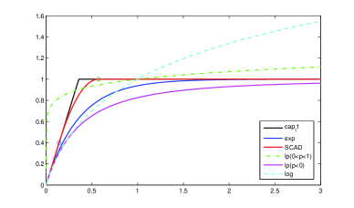
Figure 1: Graphs of approximation functions. Except $\ell_{p}$-norm($0<p<1$) and PiL, the others have the same derivative at 0. Here $\theta_{log}=10$ for Log, $a=4$ for SCAD, $p=-2$ for $\ell_{p}$-norm($p<0$). For $\ell_{p}$-norm($0<p<1$), $\epsilon=10^{-9}$ and $p=0.2$. For PiL, $a=5$ and $\theta_{PiL}=a\theta_{exp}$.

Now, we give a deeper study on Capped-$\ell_{1}$ approximation. Using exact penalty techniques related to $\ell_{0}$-norm developed in ([79, 70, 52]) we prove a much stronger result for this approximation, that is the approximation problem (12) is equivalent to the original problem with appropriate parameters $\theta$ when $K$ is a compact polyhedral convex set (this case quite often occurs in applications, in particular in machine learning contexts). Furthermore, when $K$ is a box, we show (directly, without using the exact penalty techniques) that the Capped-$\ell_{1}$ approximation problem is equivalent to the original problem and we compute an exact value $\theta_{0}$ such that the equivalence holds for all $\theta>\theta_{0}$.

5 A deeper study on Capped-$\ell_{1}$ approximation problems

5.1 Link between approximation and exact penalty approaches

Thanks to exact continuous reformulation via penalty techniques, we shall prove that, with some sparse inducing functions, the approximate problem is equivalent to the original problem. First of all, let us recall exact penalty techniques related to $\ell_{0}$-norm ([79, 70]).

5.1.1 Continuous reformulation via exact penalty techniques

Denote by $e$ the vector of ones in the appropriate vector space. We suppose that $K$ is bounded in the variable $x$, i.e. $K\subset\Pi_{i=1}^{n}[a_{i},b_{i}]\times\mathbb{R}^{m}$ where $a_{i},b_{i}\in$ $\mathbb{R}$ such that $a_{i}\leq 0<b_{i}$ for $i=1,...,n.$ Let $c_{i}:=\max\{\left|x_{i}\right|:x_{i}\in[a_{i},b_{i}]\}=\max\{\left|a_{i}\right|,\left|b_{i}\right|\}$ for $i=1,...,n.$ Define the binary variable $u_{i}\in\left\{0,1\right\}$ as

$$u_{i}=\left|x_{i}\right|_{0}=\begin{cases}1\text{ if }x_{i}\neq 0\\ 0\text{ if }x_{i}=0,\end{cases}\qquad\forall i=1...n.$$ (25)

Then (1) can be reformulated as

$$\alpha:=\inf\{f(x,y)+\lambda e^{T}u:(x,y)\in K,u\in\{0,1\}^{n},\left|x_{i}\right|\leq c_{i}u_{i},\text{ }i=1,...,n\},$$ (26)

Let $p(u)$ be the penalty function defined by

$$p(u):=\sum\limits_{i=1}^{n}\min\{u_{i},1-u_{i}\}\text{.}$$ (27)

Then (1) can be rewritten as

$$\alpha=\inf\{f(x,y)+\lambda e^{T}u:(x,y)\in K,u\in[0,1]^{n},\left|x_{i}\right|\leq c_{i}u_{i},\text{ }i=1,...,n,\text{ }p(u)\leq 0\},$$ (28)

which leads to the corresponding penalized problems $(\tau$ being the positive penalty parameter)

$$\alpha(\tau):=\inf\{f(x,y)+\lambda e^{T}u+\tau p(u):(x,y)\in K,u\in[0,1]^{n},\left|x_{i}\right|\leq c_{i}u_{i},\text{ }i=1,...,n\}.$$ (29)

It has been shown in [79, 70] that there is $\tau_{0}\geq 0$ such that for every $\tau>\tau_{0}$ problems (1) and (29) are equivalent, in the sense that they have the same optimal value and $(x^{\ast},y^{\ast})\in K$ is a solution of (1) iff there is $u^{\ast}\in\left\{0,1\right\}^{n}$ such that $(x^{\ast},y^{\ast},u^{\ast})$ is a solution of (29).

It is clear that if the function $f(x,y)$ is a DC function on $K$ then (28) is a DC program.

Let us state now the link between the continuous problem (29) and the Capped-$\ell_{1}$ approximation problem.

5.1.2 Link between (29) and Capped-$\ell_{1}$ approximation problem

The Capped-$\ell_{1}$ approximation is defined by:

$$\Psi_{{}_{\theta}}(x):=\sum_{i=1}^{n}r_{{}_{cap}}(x_{i}),\forall x=(x_{i})\in\mathbb{R}^{n},\text{ with }r_{cap}(t):=\min\{\theta\left|t\right|,1\},\text{ }t\in\mathbb{R}.$$ (30)

We will demonstrate that the resulting approximate problem of (1), namely

$$\beta(\theta):=\inf\left\{f(x,y)+\lambda\sum_{i=1}^{n}r_{cap}\left(x_{i}\right):(x,y)\in K\right\}$$ (31)

is equivalent to the penalized problem (29) with suitable values of parameters $\lambda,$ $\tau$ and $\theta$.

Let $M=\max\{c_{i}:i=1,\dots,n\}$, consider the problem (29) in the form

$$\alpha(\tau):=\inf\{f(x,y)+\lambda e^{T}u+\tau p(u):(x,y)\in K,u\in[0,1]^{n},|x_{i}|\leq Mu_{i},\leavevmode\nobreak\ i=1,\dots,n\}.$$ (32)

Let $\varsigma:\mathbb{R\rightarrow R}$ be the function defined by $\varsigma(t)=\min\{t,1-t\}.$ Then $p(u)=\sum_{i=1}^{n}\varsigma(u_{i})$ and the problem (32) can be rewritten as

$$\alpha(\tau):=\inf\left\{f(x,y)+\lambda\sum_{i=1}^{n}\left(u_{i}+\frac{\tau}{\lambda}\varsigma(u_{i})\right):(x,y)\in K,\frac{|x_{i}|}{M}\leq u_{i}\leq 1,\leavevmode\nobreak\ i=1,\dots,n\right\},$$ (33)

or again

$$\alpha(\tau):=\inf\left\{f(x,y)+\lambda\sum_{i=1}^{n}\pi\left(u_{i}\right):(x,y)\in K,\frac{|x_{i}|}{M}\leq u_{i}\leq 1,\leavevmode\nobreak\ i=1,\dots,n\right\}$$ (34)

where $\pi:\mathbb{R\rightarrow R}$ be the function defined by $\pi(t):=t+\frac{\tau}{\lambda}\varsigma(t).$

Proposition 3.

Let $\theta:=\frac{\tau+\lambda}{\lambda M}.$ For all $\tau\geq\lambda$ problems (34) and (31) are equivalent in the following sense: $(x^{\ast},y^{\ast})$ is an optimal solution of (31) iff $(x^{\ast},y^{\ast},u^{\ast})$ is an optimal solution of (34), where $u_{i}^{\ast}\in\left\{\frac{|x_{i}^{\ast}|}{M},1\right\}\$such that $\pi(u_{i}^{\ast})=r_{cap}(x_{i}^{\ast})$ for $i=1,\dots,n.$ Moreover, $\alpha(\tau)=\beta(\theta)$.

Proof.

If $(x^{\ast},y^{\ast},u^{\ast})$ is an optimal solution of (34), then $u_{i}^{\ast}$ is an optimal solution of the following problem, for every $i=1,\dots,n$

$$\ \min\left\{\pi(u_{i}):\frac{|x_{i}^{\ast}|}{M}\leq u_{i}\leq 1\right\}.$$ (35)

Since $\varsigma$ is a concave function, so is $\pi$. Consequently

$$\min\left\{\pi(u_{i}):\frac{|x_{i}^{\ast}|}{M}\leq u_{i}\leq 1\right\}=\min\left\{\pi\left(\frac{|x_{i}^{\ast}|}{M}\right),\pi(1)\right\}=\min\left\{\left(1+\frac{\tau}{\lambda}\right)\frac{|x_{i}^{\ast}|}{M},1\right\}=r_{cap}(x_{i}^{\ast}).$$

For an arbitrary $(x,y)\in K$, we will show that

$$f(x^{\ast},y^{\ast})+\lambda\sum_{i=1}^{n}r_{cap}(x_{i}^{\ast})\leq f(x,y)+\lambda\sum_{i=1}^{n}r_{cap}(x_{i}).$$ (36)

By the assumption that $(x^{\ast},y^{\ast},u^{\ast})$ is an optimal solution of (34), we have

$$f(x^{\ast},y^{\ast})+\lambda\sum_{i=1}^{n}\pi(u_{i}^{\ast})\leq f(x,y)+\lambda\sum_{i=1}^{n}\pi(u_{i})$$ (37)

for any feasible solution $(x,y,u)$ of (34). Let   

$$u_{i}^{x}\in\arg\min\left\{\pi(\xi)\ :\xi\in\left\{\frac{|x_{i}|}{M},1\right\}\right\}\subset\arg\min\left\{\pi(\xi):\frac{|x_{i}|}{M}\leq\xi\leq 1\right\},$$

for all $i=1,\dots,n$. Then $(x,y,u^{x})$ is a feasible solution of (32) and

$$\pi(u_{i}^{x})=\min\left\{\pi(\xi):\frac{|x_{i}|}{M}\leq\xi\leq 1\right\}\ =r_{cap}(x_{i}),\quad\forall i=1,\dots,n.$$

Combining (37) in which $u_{i}$ is replaced by $u_{i}^{x}$ and the last equation we get (36), which implies that $(x^{\ast},y^{\ast})$ is an optimal solution of (31).

Conversely, if $(x^{\ast},y^{\ast})$ is a solution of (31), and let $u_{i}^{\ast}\in\left\{\frac{|x_{i}^{\ast}|}{M},1\right\}\$such that $\pi(u_{i}^{\ast})=r_{cap}(x_{i}^{\ast})$ for $i=1,\dots,n.$ Then $(x^{\ast},y^{\ast},u^{\ast})$ is a feasible solution of (34) and for an arbitrary feasible solution $(x,y,u)$ of (34), we have

$$f(x,y)+\lambda\sum_{i=1}^{n}\pi(u_{i})\geq f(x,y)+\lambda\sum_{i=1}^{n}r_{cap}(x_{i})$$

$$\geq f(x^{\ast},y^{\ast})+\lambda\sum_{i=1}^{n}r_{cap}(x_{i}^{\ast})=f(x^{\ast},y^{\ast})+\lambda\sum_{i=1}^{n}\pi(u^{*}_{i}).$$

Thus, $(x^{\ast},y^{\ast},u^{\ast})$ is an optimal solution of (34). The equality $\alpha(\tau)=\beta(\theta)$ is immediately deduced from the equality $\pi(u_{i}^{\ast})=r_{cap}(x_{i}^{\ast}).$   

We conclude from the above results that for $\theta=\frac{\tau+\lambda}{\lambda M}$ with $\tau>\max\{\lambda,\tau_{0}\}$, or equivalently $\theta>\theta_{0}:=\max\{\frac{2}{M},\frac{\tau_{0}+\lambda}{\lambda M}\}$, the approximate problem (31) is equivalent to the origial problem (1). The result justifies the goodness of the Capped-$\ell_{1}$ approximation studied in Section 4 above.

5.2 A special case: link between the original problem (1) and Capped-$\ell_{1}$ approximation problem

In particular, for a special structure of $K$, we get the following result.

Proposition 4.

Suppose that $K=\prod_{i=1}^{n}[-l_{i},l_{i}]\times Y\leavevmode\nobreak\ (0\leq l_{i}\leq+\infty\leavevmode\nobreak\ \forall i,Y\subset\mathbb{R}^{m})$ and $\kappa>0$ is a constant satisfying

$$|f(x,y)-f(x^{\prime},y)|\leq\kappa\|x-x^{\prime}\|_{2}\quad\forall(x,y),(x^{\prime},y)\in K,\|x-x^{\prime}\|_{0}\leq 1.$$ (38)

Then for $\theta>\frac{\kappa}{\lambda}$, the problems (1) and (31) are equivalent.

Proof.

We observe that if $(x,y)\in K$ such that $0<|x_{i_{0}}|<\frac{1}{\theta}$ for some $i_{0}$, let $(x^{\prime},y)\in K$ determined by $x^{\prime}_{i}=x_{i}\leavevmode\nobreak\ \forall i\neq i_{0}$ and $x^{\prime}_{i_{0}}=0$, then

$$f(x,y)+\lambda\Phi(x)>f(x^{\prime},y)+\lambda\Phi(x^{\prime}),$$

where $\Phi(x)=\sum_{i=1}^{n}r_{cap}(x_{i})$. Indeed, this inequality follows the facts that

$$|f(x,y)-f(x^{\prime},y)|\leq\kappa\|x-x^{\prime}\|=\kappa|x_{i_{0}}|$$

and

$$\Phi(x)-\Phi(x^{\prime})=r_{cap}(x_{i_{0}})=\theta|x_{i_{0}}|>\frac{\kappa}{\lambda}|x_{i_{0}}|.$$

For $x\in\mathbb{R}^{n}$, we define $t^{x}\in\mathbb{R}^{n}$ by $t^{x}_{i}=0$ if $|x_{i}|<\frac{1}{\theta}$ and $t^{x}_{i}=x_{i}$ otherwise. By applying the above observation, for any $(x,y)\in K$, we have

$$f(x,y)+\lambda\Phi(x)\geq f(t^{x},y)+\lambda\Phi(t^{x}).$$

The equality holds iff $|x_{i}|\geq\frac{1}{\theta}\leavevmode\nobreak\ \forall i\in\mathrm{supp}(x)$.

Therefore, if $(x^{*},y^{*})$ is a solution of (31), we have $|x^{*}_{i}|\geq\frac{1}{\theta}\leavevmode\nobreak\ \forall i\in\mathrm{supp}(x^{*})$. Then, for any $(x,y)\in K$,

$$f(x,y)+\lambda\|x\|_{0}\geq f(x,y)+\lambda\Phi(x)\geq f(x^{*},y^{*})+\lambda\Phi(x^{*})=f(x^{*},y^{*})+\lambda\|x^{*}\|_{0}.$$

This means that $(x^{*},y^{*})$ is a solution of (1).

Conversely, assume that $(x^{*},y^{*})$ is a solution of (1). Then for any $(x,y)\in K$, we have

$$f(x,y)+\lambda\Phi(x) \geq f(t^{x},y)+\lambda\Phi(t^{x})=f(t^{x},y)+\lambda\|t^{x}\|_{0}$$

$$\geq f(x^{*},y^{*})+\lambda\|x^{*}\|_{0}\geq f(x^{*},y^{*})+\lambda\Phi(x^{*}).$$

Thus, $(x^{*},y^{*})$ is a solution of (31).    

For the problem of feature selection in SVM, we consider the loss function

$$f(x,b)=(1-\lambda)\left(\frac{1}{N_{A}}\|\max\{0,-Ax+eb+e\}\|_{1}+\frac{1}{N_{B}}\|\max\{0,Bx-eb+e\}\|_{1}\right),$$

(cf. Sect. 7 for definition of notations).

It is easy to prove that for $u\in\mathbb{R}^{n}$, $\iota\in\mathbb{R}$ and $i\in\{1,\dots,n\}$, we have

$$|\max\{0,\langle u,x\rangle+\iota\}-\max\{0,\langle u,x^{\prime}\rangle+\iota\}|\leq|u|_{i}|x_{i}-x_{i}^{\prime}|,$$

for all $x,x^{\prime}\in\mathbb{R}^{n}$ such that $x_{j}=x_{j}^{\prime}\leavevmode\nobreak\ \forall j\neq i$. Therefore, for $\kappa=(1-\lambda)\max\limits_{i=1,\dots,n}\left\{\frac{1}{N_{A}}\sum\limits_{k=1}^{N_{A}}|A_{ki}|+\frac{1}{N_{B}}\sum\limits_{l=1}^{N_{B}}|B_{li}|\right\}$, we have

$$|f(x,b)-f(x^{\prime},b)|\leq\kappa\|x-x^{\prime}\|,\quad\forall b\in\mathbb{R},\forall x,x^{\prime}\in\mathbb{R}^{n}\text{ s.t. }\|x-x^{\prime}\|_{0}\leq 1.$$

By virtue of Proposition 4, in the case of feature selection in SVM, for $\theta>\theta^{\ast}:=\frac{\kappa}{\lambda}$, the problems (1) and (31) are equivalent.

5.3 Extension to other approximations

Proposition 5.

i) Suppose that $\sigma$ is a function on $\mathbb{R}$ satisfying

$$r_{cap}(t)\leq\sigma(t)\leq s(t)=\begin{cases}0,&\text{if }t=0,\\ 1,&\text{otherwise},\end{cases}$$

for some $\theta_{cap}>\theta_{0}$. Then, the problems (1) and

$$\inf\{f(x,y)+\lambda\sum_{i=1}^{n}\sigma(x_{i}):(x,y)\in K\}$$ (39)

are equivalent.
ii) In particular, if $\theta_{scad}>a\theta_{0}$ then for all $\tau\geq\lambda$ the approximate problem

$$\inf\{f(x,y)+\lambda\sum_{i=1}^{n}r_{scad}(x_{i}):(x,y)\in K\}$$

is equivalent to (1).

Proof.

As discussed before, since $\theta_{cap}>\theta_{0}$, the problems (1) and (31) are equivalent. Moreover, if $(x^{*},y^{*})$ is a common solution then

$$f(x^{*},y^{*})+\lambda\sum_{i=1}^{n}r_{cap}(x^{*}_{i})=f(x^{*},y^{*})+\lambda\|x^{*}\|_{0}.$$

Then i) is trivial by the fact that

$$f(x,y)+\lambda\sum_{i=1}^{n}r_{cap}(x_{i})\leq f(x,y)+\lambda\sum_{i=1}^{n}\sigma(x_{i})\leq f(x,y)+\lambda\|x\|_{0},\quad\forall(x,y).$$

ii) is a direct consequence of i) and Propositions 3 and (24).    

6 DCA for solving the problem (12)

In this section, we will omit the parameter $\theta$ when this doesn’t cause any ambiguity.

Usual sparsity-inducing functions are concave, increasing on $[0,+\infty)$. Therefore, first we present three variants of DCA for solving the problem (12) when $r$ is concave on $[0,+\infty)$. We also suppose that $r$ has the right derivative at $0$, denoted by $r^{\prime}(0)$, so $\partial(-r)(0)=\{-r^{\prime}(0)\}$.

First, we consider the approximate problem (12).

6.1 The first DCA scheme for solving the problem (12)

We propose the following DC decomposition of $r$:

$$r(t)=\eta|t|-(\eta|t|-r(t))\quad\forall t\in\mathbb{R},$$ (40)

where $\eta$ is a positive number such that $\psi(t)=\eta|t|-r(t)$ is convex. The next result gives a sufficient condition for the existence of such a $\eta$.

Proposition 6.

Suppose that $r$ is a concave function on $[0,+\infty)$ and the (right) derivative at 0, $r^{\prime}(0)$, is well-defined. Let $\eta\geq r^{\prime}(0)$. Then $\psi(t)=\eta|t|-r(|t|)$ is a convex function on $\mathbb{R}$.

Proof.

Since $r$ is concave on $[0,+\infty)$, the function $\eta|t|-r(t)$ is convex on $(0,+\infty)$ and on $(-\infty,0)$. Hence it suffices to prove that for any $t_{1}>0,t_{2}<0$ and $\alpha,\beta\in(0,1)$ such that $\alpha+\beta=1$, we have

$$\psi\left(\alpha t_{1}+\beta t_{2}\right)\leq\alpha\psi(t_{1})+\beta\psi(t_{2}).$$ (41)

Without loss of generality, we assume that $\alpha|t_{1}|\geq\beta|t_{2}|$. Then (41) is equivalent to

$$\eta(\alpha|t_{1}|-\beta|t_{2}|)-2r\left(\alpha|t_{1}|-\beta|t_{2}|\right)\leq\eta(\alpha|t_{1}|+\beta|t_{2}|)-\alpha r(|t_{1}|)-\beta r(|t_{2}|)$$

which can be equivalently written as

$$\alpha r(|t_{1}|)+\beta r(|t_{2}|)-r\left(t_{0}\right)\leq 2\eta\beta|t_{2}|,$$ (42)

where $t_{0}=\alpha|t_{1}|-\beta|t_{2}|\geq 0$. Let $\mu\in\mathbb{R}$ such that $-\mu\in\partial(-r(t_{0}))$. Since $r$ is concave on $[0,+\infty)$, we have

$$\alpha r(|t_{1}|)+\beta r(|t_{2}|)-r\left(t_{0}\right)\leq r\left(\alpha|t_{1}|+\beta|t_{2}|\right)-r\left(t_{0}\right)\leq 2\mu\beta|t_{2}|.$$

Hence (42) holds when $\mu\leq\eta$. By the concavity of $r$, we have

$$r\left(\frac{t_{0}}{2}\right)\leq r(0)+r^{\prime}(0)\frac{t_{0}}{2},\quad\text{and}\quad r\left(\frac{t_{0}}{2}\right)\leq r(t_{0})-\mu\frac{t_{0}}{2},$$

therefore

$$(z-r^{\prime}(0))t_{0}\leq r(0)+r(t_{0})-2r\left(\frac{t_{0}}{2}\right)\leq 0.$$

This and the condition $r^{\prime}(0)\leq\eta$ imply that $\mu\leq r^{\prime}(0)\leq\eta$. The proof is then complete.    

With $\eta\geq r^{\prime}(0)$, a DC formulation of the problem (12) is given by

$$\min_{x,y}\{F_{r}(x,y):=G_{1}(x,y)-H_{1}(x,y)\},$$ (43)

where

$$G_{1}(x,y)=\chi_{K}(x,y)+g(x,y)+\lambda\eta\|x\|_{1},\leavevmode\nobreak\ H_{1}(x,y)=h(x,y)+\lambda\sum_{i=1}^{n}\left(\eta|x_{i}|-r(x_{i})\right),$$

and $g,h$ are DC components of $f$.

By the definition $\psi(t)=\eta|t|-r(t)\leavevmode\nobreak\ \forall t\in\mathbb{R}$, we have

$$\partial\psi(t)=\eta+\partial(-r)(t)\text{ if }t>0,\>-\eta-\partial(-r)(-t)\text{ if }t<0,\>\left[-\eta+r^{\prime}(0),\eta-r^{\prime}(0)\right]\text{ if }t=0.$$ (44)

Following the generic DCA scheme described in Section 2, DCA applied on (43) is given by Algorithm 1 below.

Algorithm 1 DCA for solving (12) (DCA1)

  Initialize $(x^{0},y^{0})\in K$, $k\leftarrow 0$

  repeat

     1. Compute $(\overline{x}^{k},\overline{y}^{k})\in\partial h(x^{k},y^{k})$ and $\overline{z}^{k}_{i}\in\lambda\partial\psi(x^{k}_{i})\leavevmode\nobreak\ \forall i=1,\dots,n$ via (44).

     2. Compute

$$(x^{k+1},y^{k+1})\in\arg\min_{(x,y)\in K}\left\{g(x,y)-\langle\overline{x}^{k},x\rangle-\langle\overline{y}^{k},y\rangle+\lambda\eta\|x\|_{1}-\langle\overline{z}^{k},x\rangle\right\}$$

     3. $k\leftarrow k+1$.

  until Stopping criterion

Instances of Algorithm 1 can be found in our previous works [42, 43, 65] using exponential concave, SCAD or Capped$-\ell_{1}$ approximations (see Table 2). Note that for usual sparse inducing functions given in Table 2, this DC decomposition is nothing but that given in Table 1, i.e. $\varphi(t)=\eta|t|$.

Table 2: Choice of $\eta$ and expression of $\overline{z}_{i}^{k}\in\lambda\partial\psi(x_{i}^{k})$ in Algorithm 1 and related works.

$r$	$\eta$	$\overline{z}_{i}^{k}\in\lambda\partial\psi(x_{i}^{k})$	Related works	Context
$r_{exp}$	$\theta$	$\mathrm{sign}(x_{i}^{k})\lambda\theta\left(1-e^{-\theta|x_{i}^{k}|}\right)$	[42]	Feature selection in SVMs
			[65]	Learning sparse classifiers
$r_{\ell_{p}^{+}}$	$\frac{\epsilon^{1/\theta-1}}{\theta}$	$\mathrm{sign}(x_{i}^{k})\frac{\lambda}{\theta}\left[\epsilon^{1/\theta-1}-(|x_{i}^{k}|+\epsilon)^{1/\theta-1}\right]$
$r_{\ell_{p}^{-}}$	$-p\theta$	$-\mathrm{sign}(x_{i}^{k})\lambda p\theta\left[1-(1+\theta|x^{k}_{i}|)^{p-1}\right]$
$r_{log}$	$\frac{\theta}{\log(1+\theta)}$	$\mathrm{sign}(x_{i}^{k})\frac{\lambda\theta^{2}|x^{k}_{i}|}{\log(1+\theta)(1+\theta|x^{k}_{i}|)}$
$r_{scad}$	$\frac{2\theta}{a+1}$	$\begin{cases}0&|x_{i}^{k}|\leq\frac{1}{\theta}\\ \mathrm{sign}(x_{i}^{k})\frac{2\lambda\theta(\theta|x_{i}^{k}|-1)}{a^{2}-1}&\frac{1}{\theta}<|x_{i}^{k}|<\frac{a}{\theta}\\ \mathrm{sign}(x_{i}^{k})\frac{2\lambda\theta}{a+1}&\text{otherwise}\end{cases}$	[43]	Feature selection in SVMs
$r_{cap}$	$\theta$	$\begin{cases}0&|x_{i}^{k}|\leq\frac{1}{\theta}\\ \mathrm{sign}(x_{i}^{k})\lambda\theta&\text{otherwise}\end{cases}$	[65]	Learning sparse classifiers

Now we consider the approximate problem (13) and introduce a DCA scheme that includes all standard algorithms of reweighted-$\ell_{1}$-type for sparse optimization problem (10).

6.2 DCA2 - Relation with reweighted-$\ell_{1}$ procedure

The problem (13) can be written as a DC program as follows

$$\min_{x,y,z}\{\overline{F}_{r}(x,y,z):=G_{2}(x,y,z)-H_{2}(x,y,z)\},$$ (45)

where

$$G_{2}(x,y,z)=\chi_{\Omega_{1}}(x,y,z)+g(x,y),\leavevmode\nobreak\ H_{2}(x,y,z)=h(x,y)+\lambda\sum_{i=1}^{n}(-r)(z_{i}),$$

and $g,h$ are DC components of $f$ as stated in (11).

Assume that $(x^{k},y^{k},z^{k})\in\Omega_{1}$ is the current solution at iteration $k$. DCA applied to DC program (45) updates $(x^{k+1},y^{k+1},z^{k+1})\in\Omega_{1}$ via two steps:

1. Step 1: compute $(\overline{x}^{k},\overline{y}^{k})\in\partial h(x^{k},y^{k})$, and $\overline{z}_{i}^{k}\in\lambda\partial(-r)(z_{i}^{k})\leavevmode\nobreak\ \leavevmode\nobreak\ \forall i=1,\dots,n$.

2. Step 2: compute

   $$(x^{k+1},y^{k+1},z^{k+1}) \in \arg\min\left\{G_{2}(x,y,z)-\langle\overline{x}^{k},x\rangle-\langle\overline{y}^{k},y\rangle-\langle\overline{z}^{k},z\rangle\right\}$$

   $$= \mathop{\arg\min}_{(x,y,z)\in\Omega_{1}}\left\{g(x,y)-\langle\overline{x}^{k},x\rangle-\langle\overline{y}^{k},y\rangle+\langle-\overline{z}^{k},z\rangle\right\}.$$

Since $r$ is increasing, we have $-\overline{z}^{k}\geq 0$. Thus, updating $(x^{k+1},y^{k+1},z^{k+1})$ can be done as follows

$$\begin{cases}(x^{k+1},y^{k+1})\in\arg\min_{(x,y)\in K}\left\{g(x,y)-\langle\overline{x}^{k},x\rangle-\langle\overline{y}^{k},y\rangle+\langle-\overline{z}^{k},|x|\rangle\right\}\\ z_{i}^{k+1}=|x_{i}^{k+1}|\leavevmode\nobreak\ \leavevmode\nobreak\ \forall i.\end{cases}$$

DCA for solving the problem (13) can be described as in Algorithm 2 below.

Algorithm 2 DCA for solving (13) (DCA2)

  Initialize $(x^{0},y^{0},z^{0})\in\Omega_{1}$, $k\leftarrow 0$

  repeat

     1. Compute $(\overline{x}^{k},\overline{y}^{k})\in\partial h(x^{k},y^{k})$, $\overline{z}^{k}_{i}\in-\lambda\partial(-r)(z^{k}_{i})\leavevmode\nobreak\ \leavevmode\nobreak\ \forall i=1,\dots,n$.

     2. Compute

$$(x^{k+1},y^{k+1})\in\mathop{\arg\min}_{(x,y)\in K}\left\{g(x,y)-\langle\overline{x}^{k},x\rangle-\langle\overline{y}^{k},y\rangle+\langle\overline{z}^{k},|x|\rangle\right\}$$

$$z^{k+1}_{i}=|x^{k+1}_{i}|\leavevmode\nobreak\ \forall i=1,\dots,n.$$

     3. $k\leftarrow k+1$.

  until Stopping criterion

If the function $f$ in (10) is convex, we can chose DC components of $f$ as $g=f$ and $h=0$. Then $(\overline{x}^{k},\overline{y}^{k})=0\leavevmode\nobreak\ \forall k$. In this case, the step 2 in Algorithm 2 becomes

$$(x^{k+1},y^{k+1})\in\arg\min_{(x,y)\in K}\left\{f(x,y)+\sum_{i=1}^{n}\overline{z}_{i}^{k}|x_{i}|\right\}.$$ (46)

We see that the problem (46) has the form of a $\ell_{1}$-regularization problem but with different weights on components of $|x_{i}|$. So Algorithm 2 iteratively solves the weighted–$\ell_{1}$ problem (46) with an update of the weights $\overline{z}_{i}^{k}$ at each iteration $k$. The expression of weights $\overline{z}_{i}^{k}$ according to approximation functions are given in Table 3.

The update rule (46) covers standard algorithms of reweighted–$\ell_{1}$–type for sparse optimization problem (10) (see Table 3). Some algorithms such as the two–stage $\ell_{1}$ ([83]) and the adaptive Lasso ([86]) only run in a few iterations (typically two iterations) and their reasonings bear a heuristic character. The reweighted–$\ell_{1}$ algorithm proposed in [8] lacks of theoretical justification for the convergence.

Table 3: Expression of $\overline{z}^{k}_{i}$ in Algorithm 2 and relation with reweighted-$\ell_{1}$ algorithms.

Function $r$	expression of $\overline{z}^{k}_{i}$	Related works	Context
$r_{exp}$	$\lambda\theta e^{-\theta z^{k}_{i}}$	SLA ([4])	Feature selection in SVMs
$r_{\ell_{p}^{+}}$	$\dfrac{\lambda}{\theta(z^{k}_{i}+\epsilon)^{1-1/\theta}}$	Adaptive Lasso ([86])	Linear regression
$r_{\ell_{p}^{-}}$	$-\lambda p\theta(1+\theta z^{k}_{i})^{p-1}$
$r_{scad}$	$\begin{cases}\frac{2\lambda\theta}{a+1}&\text{if }z^{k}_{i}\leq\frac{1}{\theta}\\ 0&\text{if }z^{k}_{i}\geq\frac{a}{\theta}\\ \frac{\lambda\theta(a-\theta z^{k}_{i})}{a^{2}-1}&\text{otherwise}\end{cases}$	LLA (Local Linear Approximation) ([87])
$r_{cap}$	$\begin{cases}\lambda\theta&\text{if }z^{k}_{i}\leq 1/\theta\\ 0&\text{otherwise}\end{cases}$	Two-stage $\ell_{1}$ ([83])
$r_{log}$	$\dfrac{\lambda\theta}{\log(1+\theta)(1+\theta z^{k}_{i})}$	Adaptive Lasso ([86]); Reweighted $\ell_{1}$ ([8])	Sparse signal reconstruction

Next, we introduce a slight perturbation of the formulation (12) and develop the third DCA scheme that includes existing algorithms of reweighted–$\ell_{2}$–type for sparse optimization problem (10).

6.3 DCA3 - Relation with reweighted-$\ell_{2}$ procedure

To avoid the singularity at $0$ of the function $r(t^{1/2}),t\geq 0$, we add $\epsilon>0$ and consider the perturbation problem of (12) which is defined by

$$\begin{cases}\min_{x,y}&\tilde{F}_{r}(x,y):=f(x,y)+\lambda\sum_{i=1}^{n}r((|x_{i}|^{2}+\epsilon)^{1/2})\\ s.t.&(x,y)\in K,\end{cases}\quad\epsilon>0.$$ (47)

Clearly (47) becomes (12) when $\epsilon=0$. The problem (47) is equivalent to

$$\min_{(x,y,z)\in\Omega_{2}}\hat{F}_{r}(x,y,z):=f(x,y)+\lambda\sum_{i=1}^{n}r((z_{i}+\epsilon)^{1/2}),$$ (48)

where $\Omega_{2}=\{(x,y,z):(x,y)\in K;\quad|x_{i}|^{2}\leq z_{i}\leavevmode\nobreak\ \forall i\}$. The last problem is a DC program of the form

$$\min_{x,y,z}\{\hat{F}_{r}(x,y,z):=G_{3}(x,y,z)-H_{3}(x,y,z)\},$$ (49)

where

$$G_{3}(x,y,z)=\chi_{\Omega_{2}}(x,y,z)+g(x,y),\leavevmode\nobreak\ H_{3}(x,y,z)=h(x,y)+\lambda\sum_{i=1}^{n}(-r)((z_{i}+\epsilon)^{1/2}),$$

and $g,h$ are DC components of $f$ as stated in (11). Note that, since the functions $r$ and $(t+\epsilon)^{1/2}$ are concave, increasing on $[0,+\infty)$, $(-r)((t+\epsilon)^{1/2})$ is a convex function on $[0,+\infty)$.

Let $(x^{k},y^{k},z^{k})\in\Omega_{2}$ be the current solution at iteration $k$. DCA applied to DC program (49) updates $(x^{k+1},y^{k+1},z^{k+1})\in\Omega_{2}$ via two steps:

1. Step 1: compute $(\overline{x}^{k},\overline{y}^{k})\in\partial h(x^{k},y^{k})$, and $\overline{z}_{i}^{k}\in\frac{\lambda}{2(z_{i}^{k}+\epsilon)^{1/2}}\partial(-r)((z_{i}^{k}+\epsilon)^{1/2})\leavevmode\nobreak\ \leavevmode\nobreak\ \forall i=1,\dots,n$.

2. Step 2: compute

   $$(x^{k+1},y^{k+1},z^{k+1}) \in \arg\min\left\{G_{3}(x,y,z)-\langle\overline{x}^{k},x\rangle-\langle\overline{y}^{k},y\rangle-\langle\overline{z}^{k},z\rangle\right\}$$

   $$= \mathop{\arg\min}_{(x,y,z)\in\Omega_{2}}\left\{g(x,y)-\langle\overline{x}^{k},x\rangle-\langle\overline{y}^{k},y\rangle+\langle-\overline{z}^{k},z\rangle\right\}$$

Since $r$ is increasing, we have $-\overline{z}^{k}\geq 0$. Thus, updating $(x^{k+1},y^{k+1},z^{k+1})$ can be done as follows

$$\begin{cases}(x^{k+1},y^{k+1})\in\mathop{\arg\min}_{(x,y)\in K}\left\{g(x,y)-\langle\overline{x}^{k},x\rangle-\langle\overline{y}^{k},y\rangle+\sum_{i=1}^{n}(-\overline{z}_{i}^{k})x_{i}^{2}\rangle\right\}\\ z_{i}^{k+1}=|x_{i}^{k+1}|^{2}\leavevmode\nobreak\ \leavevmode\nobreak\ \forall i=1,\dots,n.\end{cases}$$

DCA for solving the problem (48) can be described as in Algorithm 3 below.

Algorithm 3 DCA for solving (48) (DCA3)

  Initialize $(x^{0},y^{0},z^{0})\in\Omega_{2}$, $k\leftarrow 0$

  repeat

     1. Compute $(\overline{x}^{k},\overline{y}^{k})\in\partial h(x^{k},y^{k})$, $\overline{z}^{k}_{i}\in\frac{-\lambda}{2(z^{k}_{i}+\epsilon)^{1/2}}\partial(-r)(z^{k}_{i}+\epsilon)^{1/2})\leavevmode\nobreak\ \leavevmode\nobreak\ \forall i=1,\dots,n$.

     2. Compute

$$(x^{k+1},y^{k+1})\in\mathop{\arg\min}_{(x,y)\in K}\left\{g(x,y)-\langle\overline{x}^{k},x\rangle-\langle\overline{y}^{k},y\rangle+\sum_{i=1}^{n}\overline{z}^{k}_{i}x^{2}_{i}\right\},$$

$$z_{i}^{k+1}=|x_{i}^{k+1}|^{2}\leavevmode\nobreak\ \leavevmode\nobreak\ \forall i=1,\dots,n.$$

     3. $k\leftarrow k+1$.

  until Stopping criterion

If the function $f$ in (10) is convex, then, as before, we can chose DC components of $f$ as $g=f$ and $h=0$. Hence, in the step 1 of Algorithm 3, we have $(\overline{x}^{k},\overline{y}^{k})=0\leavevmode\nobreak\ \forall k$. In this case, the step 2 in Algorithm 3 becomes

$$(x^{k+1},y^{k+1})\in\arg\min_{(x,y)\in K}\left\{f(x,y)+\sum_{i=1}^{n}\overline{z}_{i}^{k}x_{i}^{2}\right\}.$$ (50)

Thus, each iteration of Algorithm 3 solves a weighted-$\ell_{2}$ optimization problem. The expression of weights $\overline{z}_{i}^{k}$ according to approximation functions are given in Table 4.

If $\epsilon=0$ then the update rule (50) encompasses standard algorithms of reweighted-$\ell_{2}$ type for finding sparse solution (see Table 4). However, when $\epsilon=0$ the (right) derivative at 0 of $r(t^{1/2})$ is not well-defined, that is why we take $\epsilon>0$ in our algorithm. Note also that, in LQA and FOCUSS, if at an iteration $k$ one has $x_{i}^{k}=0$ then $x_{i}^{l}=0$ for all $l\geq k,$ by the way these algorithms may converge prematurely to bad solutions.

Table 4: Expression of $\overline{z}^{k}_{i}$’s in Algorithm 3 and relation with reweighted-$\ell_{2}$ algorithms.

Function $r$	weight $\overline{z}^{k}_{i}$($t^{k}_{i}=(z^{k}_{i}+\epsilon)^{1/2}$)	Related works	Context
$r_{exp}$	$\dfrac{\lambda\theta}{2}\dfrac{e^{-\theta t^{k}_{i}}}{t^{k}_{i}}$
$r_{\ell_{p}^{+}}$	$\dfrac{\lambda}{2\theta(t^{k}_{i})^{2-\frac{1}{\theta}}}$	FOCUSS ([18, 71, 72]);	Sparse signal
$r_{\ell_{p}^{-}}$	$\dfrac{-\lambda p\theta^{p}}{2t^{k}_{i}(\frac{1}{\theta}+t^{k}_{i})^{1-p}}$	IRLS ([9])	reconstruction
$r_{log}$	$\dfrac{\lambda}{2\log(1+\theta)}\dfrac{1}{t^{k}_{i}(\frac{1}{\theta}+t^{k}_{i})}$
$r_{cap}$	$\begin{cases}\frac{\lambda\theta}{2t^{k}_{i}}&\text{if }|t^{k}_{i}|\leq\frac{1}{\theta}\\ 0&\text{otherwise}\end{cases}$
$r_{scad}$	$\begin{cases}\frac{\lambda\theta}{(a+1)t^{k}_{i}}&\text{if }t^{k}_{i}\leq\frac{1}{\theta}\\ 0&\text{if }t^{k}_{i}\geq\frac{a}{\theta}\\ \frac{\lambda\theta(-\theta t^{k}_{i}+a)}{(a^{2}-1)t^{k}_{i}}&\text{otherwise}\end{cases}$	LQA ([13, 87])	Linear regression

6.4 Discussion on the three DCA based algorithms 1, 2 and 3

Algorithm 1 seems to be the most interesting in the sense that it addresses directly the problem (12) and doesn’t need the additional variable $z$, then the subproblem has less constraints than that in Algorithms 2 and 3. Moreover, the DC decomposition (40) is more suitable since it results, in several cases, in a DC polyhedral program where both DC components are polyhedral convex (for instance, in feature selection in SVM with the approximations $r_{scad},$ $r_{cap}$) for which Algorithm 1 enjoys interesting convergence properties.

Algorithms 2 and 3 are based on two different formulations of the problem (12). In (13), we have linear constraints $|x|_{i}\leq z_{i},\leavevmode\nobreak\ i=1,\dots,n$ that lead to the subproblem of weighted–$\ell_{1}$ type. Whereas, in (47), quadratic constraints $|x|_{i}^{2}\leq z_{i},\leavevmode\nobreak\ i=1,\dots,n$ result to the subproblem of weighted–$\ell_{2}$ type. With second order terms in subproblems, Algorithm 3 is, in general, more expensive than Algorithms 1 and 2. We also see that Algorithms 1 and 2 possess nicer convergence properties than Algorithm 3. Both Algorithms 1 and 2 have finite convergence when the corresponding DC programs are polyhedral DC. While (47) can’t be a polyhedral DC program because the set $\Omega_{2}$ and the functions $r((t+\epsilon)^{1/2})$ are not polyhedral convex.

To compare the sparsity of solutions given by the algorithms, we consider the subproblems in Algorithms 1, 2, and 3 which have the form

$$\min_{(x,y)\in K}\left\{g(x,y)-\langle\overline{x}^{k},x\rangle-\langle\overline{y}^{k},y\rangle+\lambda\sum_{i=1}^{n}\nu(x_{i},x_{i}^{k})\right\}$$

where $(\overline{x}^{k},\overline{y}^{k})\in\partial h(x^{k},y^{k})$,

$$\nu(x_{i},x_{i}^{k})=\begin{cases}\nu_{1}(x_{i},x_{i}^{k})=\eta|x_{i}|-\mathrm{sign}(x_{i}^{k})(\eta-\overline{z}_{i}^{k})x_{i}+C_{i}^{k}&\text{for Algorithm \ref{DCA1}}\\ \nu_{2}(x_{i},x_{i}^{k})=\overline{z}_{i}^{k}|x_{i}|+C_{i}^{k}&\text{for Algorithm \ref{DCA2}}\\ \nu_{3}(x_{i},x_{i}^{k})=\frac{\overline{z}_{i}^{k}}{2|x_{i}^{k}|}|x_{i}|^{2}+\frac{1}{2}\overline{z}_{i}^{k}|x_{i}^{k}|+C_{i}^{k}&\text{for Algorithm \ref{DCA3}},\end{cases}$$

with $\overline{z}_{i}^{k}\in-\partial(-r)(|x_{i}^{k}|)$, $C_{i}^{k}=r(x_{i}^{k})-\overline{z}_{i}^{k}|x_{i}^{k}|$ and $\eta=r^{\prime}(0)$.

All three functions $\nu_{1}$, $\nu_{2}$ and $\nu_{3}$ attain minimum at $0$ and encourage solutions to be zero. Denote by $\nu_{-}^{\prime}(t)$ and $\nu_{+}^{\prime}(t)$ the left and right derivative at $t$ of $\nu$ respectively. We have

$$\nu_{1,-}^{\prime}(0,x_{i}^{k})=-2\eta+\overline{z}_{i}^{k},\quad\nu_{2,-}^{\prime}(0,x_{i}^{k})=-\overline{z}_{i}^{k},\quad\nu_{3,-}^{\prime}(0,x_{i}^{k})=0,$$

$$\nu_{1,+}^{\prime}(0,x_{i}^{k})=\overline{z}_{i}^{k},\quad\nu_{2,+}^{\prime}(0,x_{i}^{k})=\overline{z}_{i}^{k},\quad\nu_{3,+}^{\prime}(0,x_{i}^{k})=0.$$

We also have $\eta\geq\overline{z}_{i}^{k}$ by the concavity of $r$ on $[0,+\infty)$. Observe that if the range $[\nu_{-}^{\prime}(0),\nu_{+}^{\prime}(0)]$ is large, it encourages more sparsity. Intuitively, the values $\nu_{-}^{\prime}(0)$ and $\nu_{+}^{\prime}(0)$ reflect the slope of $\nu$ at $0$, and if the slope is hight, it forces solution to be zero. Here we have $[\nu_{3,-}^{\prime}(0,x_{i}^{k}),\nu_{3,+}^{\prime}(0,x_{i}^{k})]\subset[\nu_{2,-}^{\prime}(0,x_{i}^{k}),\nu_{2,+}^{\prime}(0,x_{i}^{k})]\subset[\nu_{1,-}^{\prime}(0,x_{i}^{k}),\nu_{1,+}^{\prime}(0,x_{i}^{k})]$. Thus, we expect that Algorithm 1 gives sparser solution than Algorithm 2, and Algorithm 2 gives sparser solution than Algorithm 3.

Figure 2: Graphs of functions: $r=1-e^{-2|x|}$, $\nu_{1}$, $\nu_{2}$ and $\nu_{3}$ with $x^{k}=0.5$.

6.5 DCA4: DCA applied on (12) with the new DC approximation

We have proposed three DCA schemes for solving (12) or its equivalent form (13) when $r$ is a concave function on $[0,+\infty)$. Consider now the general case where $r$ is a DC function satisfying Assumption 1. Hence the problem (12) can be expressed as a DC program (17) for which DCA is applicable. Each iteration of DCA applied on (17) consists of computing

- Compute $(\overline{x}^{k},\overline{y}^{k})\in\partial h(x^{k},y^{k})$ and $\overline{z}^{k}_{i}\in\lambda\partial\psi(x^{k}_{i})\leavevmode\nobreak\ \forall i=1,\dots,n$.

- Compute $(x^{k+1},y^{k+1})$ as a solution of the following convex program

$$\min_{(x,y)\in K}\left\{g(x,y)-\langle\overline{x}^{k},x\rangle-\langle\overline{y}^{k},y\rangle+\lambda\sum_{i=1}^{n}\varphi(x_{i})-\langle\overline{z}^{k},x\rangle\right\}.$$ (51)

The new approximation function $r_{PiL}$ is a DC function but not concave on $[0,+\infty).$ Hence we apply DCA4 for solving the problem (12) with $r=r_{PiL}$

$$r_{PiL}=\min\left\{1,\max\left\{0,\frac{\theta|t|-1}{a-1}\right\}\right\}=\begin{cases}0&\text{if }|t|\leq\frac{1}{\theta},\\ \frac{\theta|t|-1}{a-1}&\text{if }\frac{1}{\theta}<|t|<\frac{a}{\theta},\\ 1&\text{otherwise},\end{cases}\quad a>1.$$ (52)

DC components of $r_{PiL}$ are given by

$$\varphi_{PiL}(t):=\frac{\theta}{a-1}\max\left\{\frac{1}{\theta},|t|\right\},\leavevmode\nobreak\ \psi_{PiL}(t):=\frac{\theta}{a-1}\max\left\{\frac{a}{\theta},|t|\right\}-1\quad\forall t\in\mathbb{R},$$ (53)

that are polyhedral convex functions. Then, the problem (12) can be expressed in form of a DC program as follows

$$\min_{x,y}\{F_{r_{PiL}}(x,y):=G_{4}(x,y)-H_{4}(x,y)\},$$ (54)

where

$$G_{4}(x,y)=\chi_{K}(x,y)+g(x,y)+\lambda\sum_{i=1}^{n}\varphi_{PiL}(x_{i}),\leavevmode\nobreak\ H_{4}(x,y)=h(x,y)+\lambda\sum_{i=1}^{n}\psi_{PiL}(x_{i}),$$

and $g,h$ are DC components of $f$ as stated in (11).

At each iteration $k$, DCA applied to (54) updates $(x^{k+1},y^{k+1})$ from $(x^{k},y^{k})$ via two steps:

- Compute $(\overline{x}^{k},\overline{y}^{k})\in\partial h(x^{k},y^{k})$ and $\overline{z}^{k}_{i}\in\lambda\partial\psi_{PiL}(x^{k}_{i})\leavevmode\nobreak\ \forall i=1,\dots,n$.

- Compute $(x^{k+1},y^{k+1})$ as a solution of the following convex program

$$\min_{(x,y)\in K}\left\{g(x,y)-\langle\overline{x}^{k},x\rangle-\langle\overline{y}^{k},y\rangle+\frac{\lambda\theta}{a-1}\sum_{i=1}^{n}\max\left\{\frac{1}{\theta},|x_{i}|\right\}-\langle\overline{z}^{k},x\rangle\right\}.$$ (55)

Calculation of $\overline{z}_{i}^{k}\leavevmode\nobreak\ (i=1,\dots,n)$ is given by

$$\overline{z}_{i}^{k}=\begin{cases}\frac{\lambda\theta}{a-1}&\text{if }x_{i}^{k}>\frac{a}{\theta}\\ \frac{-\lambda\theta}{a-1}&\text{if }x_{i}^{k}<\frac{-a}{\theta}\\ 0&\text{otherwise}.\end{cases}$$ (56)

Furthermore, (55) is equivalent to

$$\min_{(x,y,t)\in\Omega_{3}}\left\{g(x,y)-\langle\overline{x}^{k},x\rangle-\langle\overline{y}^{k},y\rangle+\frac{\lambda\theta}{a-1}\sum_{i=1}^{n}t_{i}-\langle\overline{z}^{k},x\rangle\right\},$$ (57)

where $\Omega_{3}=\left\{(x,y,t):(x,y)\in K,\frac{1}{\theta}\leq t_{i},x_{i}\leq t_{i},-x_{i}\leq t_{i}\leavevmode\nobreak\ \forall i=1,\dots,n\right\}$.

Algorithm 4 DCA applied to (54) (DCA4)

  Initialize $(x^{0},y^{0})\in K$, $k\leftarrow 0$

  repeat

     1. Compute $(\overline{x}^{k},\overline{y}^{k})\in\partial h(x^{k},y^{k})$ and $\overline{z}^{k}_{i}\in\lambda\partial\psi_{PiL}(x^{k}_{i})\leavevmode\nobreak\ \forall i=1,\dots,n$ via (56).

     2. Solve the convex problem (57) to obtain $(x^{k+1},y^{k+1})$.

     3. $k\leftarrow k+1$.

  until Stopping criterion.

6.6 Updating $\theta$ procedure

According to consistency results, the larger $\theta$ is, the better approximate solution would be. However, from a computational point of view, with large values of $\theta$, the approximate problems are difficult and the algorithms converge often to local minimums. We can overcome this bottleneck by using an update procedure for $\theta$. Starting with a chosen value $\theta^{0}$, at each iteration $k$, we compute $(x^{k+1},y^{k+1})$ from $(x^{k},y^{k})$ by applying the DCA based algorithms with $\theta=\theta^{k}$. The sequence $\{\theta^{k}\}_{k}$ is increasing by $\theta^{k+1}=\theta^{k}+\Delta\theta^{k}$. $\Delta\theta^{k}$ can be fixed or updated during the iterations (see Experiment 1 in the next section).

7 Application to Feature selection in SVM

In this section we focus on the context of Support Vector Machines learning with two-class linear models. Generally, the problem can be formulated as follows.

Given two finite point sets $\mathcal{A}$ (with label $+1$) and $\mathcal{B}$ (with label $-1$) in $\mathbb{R}^{n}$ represented by the matrices $A\in\mathbb{R}^{N_{A}\times n}$ and $B\in\mathbb{R}^{N_{B}\times n}$, respectively, we seek to discriminate these sets by a separating hyperplane ($x\in\mathbb{R}^{n},b\in\mathbb{R)}$

$$P=\{w\in\mathbb{R}^{n}:w^{T}x=b\}$$ (58)

which uses as few features as possible. We adopt the notations introduced in [4] and consider the optimization problem proposed in [4] that takes the form ($e\in\mathbb{R}^{n}$ being the vector of ones):

$$\min_{x,b}(1-\lambda)\left(\frac{1}{N_{A}}\|\max\{0,-Ax+eb+e\}\|_{1}+\frac{1}{N_{B}}\|\max\{0,Bx-eb+e\}\|_{1}\right)+\lambda\left\|x\right\|_{0}$$ (59)

or equivalently

$$\begin{array}[]{ll}\min_{x,y,\xi,\zeta}&(1-\lambda)(\frac{1}{N_{A}}e^{T}\xi+\frac{1}{N_{B}}e^{T}\zeta)+\lambda\left\|x\right\|_{0}\\ s.t.&-Ax+eb+e\leq\xi,\ Bx-eb+e\leq\zeta,\ \xi\geq 0,\ \zeta\geq 0.\end{array}$$ (60)

The nonnegative slack variables $\xi_{j},j=1,...,N_{A}$ represent the errors of classification of $a_{j}\in\mathcal{A}$ while $\zeta_{j},j=1,...,N_{B}$ represent the errors of classification of $b_{j}\in\mathcal{B}$. More precisely, each positive value of $\xi_{j}$determines the distance between a point $a_{j}\in A$(lying on the wrong side of the bounding hyperplane $w^{T}x=b+1$ for $\mathcal{A)}$ and the hyperplane itself. Similarly for $\zeta_{j}$, $\mathcal{B}$ and $w^{T}x=b-1$. The first term of the objective function of (60) is the average error of classification, and the second term is the number of nonzero components of the vector $x$, each of which corresponds to a representative feature. Further, if an element of $x$ is zero, the corresponding feature is removed from the dataset. Here $\lambda$ is a control parameter of the trade-off between the training error and the number of selected features.

Observe that the problem (60) is a special case of (1) where the function $f$ is given by

$$f(x,b,\xi,\zeta):=(1-\lambda)\left(\frac{1}{N_{A}}e^{T}\xi+\frac{1}{N_{B}}e^{T}\zeta\right)$$ (61)

and $K$ is a polytope defined by

$$K:=\left\{(x,b,\xi,\zeta)\in\mathbb{R}^{n}\times\mathbb{R}\times\mathbb{R}_{+}^{N_{A}}\times\mathbb{R}_{+}^{N_{B}}:-Ax+eb+e\leq\xi,\ Bx-eb+e\leq\zeta\right\}.$$ (62)

Then the approximate problem takes the form

$$\min\left\{F(x,b,\xi,\zeta):=f(x,b,\xi,\zeta)+\lambda\sum_{i=1}^{n}r(x_{i}):(x,b,\xi,\zeta)\in K\right\},$$ (63)

where $r$ is one of the sparsity-inducing functions given in Table 1. This problem is also equivalent to

$$\min\left\{\overline{F}(x,b,\xi,\zeta,z):=f(x,b,\xi,\zeta)+\lambda\sum_{i=1}^{n}r(z_{i}):(x,b,\xi,\zeta,z)\in\overline{K}\right\},$$ (64)

where $\overline{K}=\left\{(x,b,\xi,\zeta,z):(x,b,\xi,\zeta)\in K,-z_{i}\leq x_{i}\leq z_{i}\leavevmode\nobreak\ \forall i=1,\dots,n\right\}$.

Note that, since $K$ is a polyhedral convex set, all the resulting approximate problems (63) with approximation functions given in Table 2 (except for $r=r_{PiL}$) are equivalent to the problem (60) in the sense of Corollary 1. More strongly, from Proposition 4, if $r=r_{cap}$ and $\theta>\theta^{*}:=\frac{1-\lambda}{\lambda}\Delta$, where

$$\Delta:=\max_{j=1,\dots,n}\left\{\frac{1}{N_{A}}\sum_{i=1}^{N_{A}}|A_{ij}|+\frac{1}{N_{B}}\sum_{i=1}^{N_{B}}|B_{ij}|\right\},$$ (65)

then the problems (60) and (63) are equivalent.

Here the function $f$ is simply linear, and DC components of $f$ is taken as $g=f$ and $h=0$. According to Algorithms 1, 2, 3 and 4, DCA for solving the problem (63) is described briefly as follows.

DCA1: For $\eta$ given in Table 2, let $\psi(t)=\eta|t|-r(t)$. At each iteration $k$, DCA1 for solving (63) consists of

- Compute $\overline{z}_{i}^{k}\in\lambda\partial\psi(x_{i}^{k})\leavevmode\nobreak\ \forall i=1,\dots,n$ as given in Table 2.

- Compute $(x^{k+1},b^{k+1},\xi^{k+1},\zeta^{k+1})$ by solving the linear program

$$\min\left\{(1-\lambda)\left(\frac{1}{N_{A}}e^{T}\xi+\frac{1}{N_{B}}e^{T}\zeta\right)+\lambda\eta\sum_{i=1}^{n}z_{i}-\langle\overline{z}^{k},x\rangle:(x,b,\xi,\zeta,z)\in\overline{K}\right\}.$$ (66)

Since $f$ is linear and $K$ is a polyhedral convex set, the first DC component $G_{1}$ in (43) is polyhedral convex. Therefore, (43) is always a polyhedral DC program. According to the convergence property of polyhedral DC programs, DCA1 applied to (63) generates a sequence $\{(x^{k},b^{k},\xi^{k},\zeta^{k})\}$ that converges to a critical point $(x^{\ast},b^{\ast},\xi^{\ast},\zeta^{\ast})$ after finitely many iterations. Furthermore, if $r=r_{cap}$ and $|x_{i}^{\ast}|\neq\frac{1}{\theta}\leavevmode\nobreak\ \forall i=1,\dots,n$, the second DC component $H_{1}$ in (43) is polyhedral convex and differentiable at $(x^{\ast},b^{\ast},\xi^{\ast},\zeta^{\ast})$. Using the DCA’s convergence property v) in Sect. 2, we deduce that $(x^{\ast},b^{\ast},\xi^{\ast},\zeta^{\ast})$ is a local solution of (63).

DCA2: At each iteration $k$, DCA2 for solving (63) consists of

- Compute $\overline{z}^{k}_{i}\in-\lambda\partial(-r)(|x_{i}^{k}|)\leavevmode\nobreak\ \forall i=1,\dots,n$ as given in Table 3.

- Compute $(x^{k+1},b^{k+1},\xi^{k+1},\zeta^{k+1})$ by solving the linear program

$$\min\left\{(1-\lambda)\left(\frac{1}{N_{A}}e^{T}\xi+\frac{1}{N_{B}}e^{T}\zeta\right)+\langle\overline{z}^{k},z\rangle:(x,b,\xi,\zeta,z)\in\overline{K}\right\}.$$

Similar to the case of DCA1 mentioned above, (45) is also a polyhedral DC program. Thus, DCA2 applied to (64) generates a sequence $\{(x^{k},b^{k},\xi^{k},\zeta^{k},|x^{k}|)\}$ that converges to a critical point $(x^{\ast},b^{\ast},\xi^{\ast},\zeta^{\ast},|x^{\ast}|)$ after finitely many iterations. Furthermore, if $r=r_{cap}$ and $|x_{i}^{\ast}|\neq\frac{1}{\theta}\leavevmode\nobreak\ \forall i=1,\dots,n$, the second DC component $H_{2}$ in (45) is polyhedral convex and differentiable at $(x^{\ast},b^{\ast},\xi^{\ast},\zeta^{\ast},|x^{\ast}|)$. Then $(x^{\ast},b^{\ast},\xi^{\ast},\zeta^{\ast},|x^{\ast}|)$ is a local solution of (64).

DCA3: At each iteration $k$, DCA3 for solving (63) consists of

- Compute $\overline{z}^{k}_{i}\in\frac{-\lambda}{2(|x_{i}^{k}|^{2}+\epsilon)^{1/2}}\partial(-r)((|x_{i}^{k}|^{2}+\epsilon)^{1/2})\leavevmode\nobreak\ \forall i=1,\dots,n$ as given in Table 4.

- Compute $(x^{k+1},b^{k+1},\xi^{k+1},\zeta^{k+1})$ by solving the quadratic convex program

$$\min\left\{(1-\lambda)\left(\frac{1}{N_{A}}e^{T}\xi+\frac{1}{N_{B}}e^{T}\zeta\right)+\sum_{i=1}^{n}\overline{z}^{k}_{i}x_{i}^{2}:(x,b,\xi,\zeta)\in K\right\}.$$

DCA4: Consider the case $r=r_{PiL}$. At each iteration $k$, DCA4 for solving (63) consists of

- Compute $\overline{z}^{k}_{i}\in\lambda\partial\psi_{PiL}(x^{k}_{i})\leavevmode\nobreak\ \forall i=1,\dots,n$ via (56).

- Compute $(x^{k+1},b^{k+1},\xi^{k+1},\zeta^{k+1})$ by solving the linear program

$$\min \left\{(1-\lambda)\left(\frac{1}{N_{A}}e^{T}\xi+\frac{1}{N_{B}}e^{T}\zeta\right)+\frac{\lambda\theta}{a-1}\sum_{i=1}^{n}t_{i}-\langle\overline{z}^{k},x\rangle\right\},$$

$$s.t. (x,b,\xi,\zeta,t)\in\overline{K},\frac{1}{\theta}\leq t_{i}\leavevmode\nobreak\ \forall i=1,\dots,n.$$

Since the second DC component $H_{4}$ in (54) is polyhedral convex, (54) is a polyhedral DC program. Thus, DCA4 applied to (63) generates a sequence $\{(x^{k},b^{k},\xi^{k},\zeta^{k})\}$ that converges to a critical point $(x^{\ast},b^{\ast},\xi^{\ast},\zeta^{\ast})$ after finitely many of iterations. Moreover, if $|x_{i}^{\ast}|\neq\frac{1}{\theta}\leavevmode\nobreak\ \forall i=1,\dots,n$, then $H_{4}$ is differentiable at $(x^{\ast},b^{\ast},\xi^{\ast},\zeta^{\ast})$. This implies that $(x^{\ast},b^{\ast},\xi^{\ast},\zeta^{\ast})$ is a local solution of (63).

The stopping criterion of our algorithms is given by

$$\|x^{k+1}-x^{k}\|+|b^{k+1}-b^{k}|+\|\xi^{k+1}-\xi^{k}\|+\|\zeta^{k+1}-\zeta^{k}\|\leq\tau(1+\|x^{k}\|+|b^{k}|+\|\xi^{k}\|+\|\zeta^{k}\|),$$

where $\tau$ is a small tolerance.

We have seen in Sect. 5 that the approximate problem using Capped-$\ell_{1}$ and SCAD approximations are equivalent to the original problem if the parameter $\theta$ is beyond a certain threshold: $\theta\geq\theta_{0}$ (cf. Proposition 3 and Proposition 5). However, the computation of such a value $\theta_{0}$ is in general not available, hence one must take large enough values for $\theta_{0}$. But, as discussed in Sect. 6.6, a large value of $\theta$ makes the approximate problem hard to solve. For the feature selection in SVM, we can compute exactly a $\theta_{0}$ as shown in (65), but it is quite large. Hence we use an updating $\theta$ procedure. On the other hand, in the DCA1 scheme, at each iteration, we have to compute $\bar{z}^{k}\in\partial\lambda\psi(x^{k})$ and when $\psi$ is not differentiable at $x^{k}$, the choice of $\bar{z}^{k}$ can influence on the efficiency of the algorithm. For Capped-$\ell_{1}$ approximation, based on the properties of this function we propose a specific way to compute $\bar{z}^{k}$. Below, we describe the updating $\theta$ procedure for DCA1 with Capped-$\ell_{1}$ approximation.

Initialization: $\Delta\theta>0,\alpha^{0}=+\infty$, $\theta^{0}=0$, $k=0$. Let $(x^{0},b^{0},\xi^{0},\zeta^{0})$ be a solution of the linear problem (63).
Repeat
1. $I=\{i:0<|x^{k}_{i}|<\alpha^{k}\}$, $\alpha^{k+1}=\begin{cases}\max\{|x^{k}_{i}|:i\in I\}&\text{if }I\neq\emptyset,\\ \alpha^{k}&\text{otherwise.}\end{cases}$
2. Compute $\theta^{k+1}=\min\left\{\theta^{*},\max\left\{\frac{1}{\alpha^{k+1}},\theta^{k}+\Delta\theta\right\}\right\}$.
3. Compute $\overline{z}^{k}$: For $i=1,\dots,n$

1. If $|x^{k}_{i}|<\alpha^{k+1}$, $\overline{z}^{k}_{i}=0$.

2. If $|x^{k}_{i}|>\alpha^{k+1}$, $\overline{z}^{k}_{i}=\text{sign}(x^{k}_{i})\lambda\theta$.

3. If $|x^{k}_{i}|=\alpha^{k+1}$, compute $F_{i}^{-}$ (resp. $F_{i}^{+}$) the left (resp. right) derivative of the function $u(x,b)$ w.r.t. the variable $x_{i}$ at $x^{k}_{i}$, where

   $$u(x,b)=(1-\lambda)\left(\frac{1}{N_{A}}\|\max\{0,-Ax+eb+e\}\|_{1}+\frac{1}{N_{B}}\|\max\{0,Bx-eb+e\}\|_{1}\right)+\lambda\sum_{j=1}^{n}r(x_{j}).$$

   Then $\overline{z}^{k}_{i}=\begin{cases}\text{sign}(x^{k}_{i})\lambda\theta^{k+1}&\text{if }x^{k}_{i}(F_{i}^{-}+F_{i}^{+})<0\\ 0&\text{ortherwise.}\end{cases}$

4. Solve the linear problem (66) with $\eta=\theta^{k+1}$ to obtain $(x^{k+1},b^{k+1},\xi^{k+1},\zeta^{k+1})$.
5. $k=k+1$.
Until: Convergence of $\{x^{k},b^{k},\xi^{k},\zeta^{k}\}$.

In the above procedure, the computation of $\overline{z}^{k}$ is slightly different from formula given in Table 2. When $|x^{k}_{i}|=\alpha^{k+1}$, $\partial r(x^{k}_{i})$ is an interval. Taking into account information of derivative of $u$ w.r.t. the variable $x_{i}$ at $x^{k}_{i}$ helps us judge which between two extreme values of $\partial r(x^{k}_{i})$ may give better decrease of algorithm.

At each iteration, the value of $\theta$ increases at least $\Delta\theta>0$ as long as it does not exceed $\theta^{*}$ – the value from which the problems (60) and (63) are equivalent. Moreover, we know that for each fixed $\theta$, DCA1 has finite convergence. Hence, the above procedure also possesses finite convergence property.

If $F(x^{k+1},b^{k+1},\xi^{k+1},\zeta^{k+1})=F(x^{k},b^{k},\xi^{k},\zeta^{k})$ then $(x^{k},b^{k},\xi^{k},\zeta^{k})$ is a critical point of (63) with $r=r_{cap}$ and $\theta=\theta^{k+1}$. In addition, if $\alpha^{k+1}=\alpha^{k}$, which means that $|x^{k}_{i}|\geq\alpha^{k}\geq\frac{1}{\theta^{k}}$ for any $i\in supp(x^{k})$, then $(x^{k},b^{k},\xi^{k},\zeta^{k})$ is a critical point of (63) for all $\theta\geq\theta^{k+1}$.

7.1 Computational experiments

7.1.1 Datasets

Numerical experiments were performed on several real-word datasets taken from well-known UCI data repository and from challenging feature-selection problems of the NIPS 2003 datasets. In Table 5, the number of features, the number of points in training and test set of each dataset are given. The full description of each dataset can be found on the web site of UCI repository and NIPS 2003.

Table 5: Datasets

Data	#features	# points in training set	# points in test set
Ionosphere	34	234	117
WPBC (24 months)	32	104	51
WPBC (60 months)	32	380	189
Breast Cancer	24481	78	19
Leukemia	7129	38	34
Arcene	10000	100	100
Gisette	5000	6000	1000
Prostate	12600	102	21
Adv	1558	2458	821

7.1.2 Set up experiments

All algorithms were implemented in the Visual C++ 2008, and performed on a PC Intel i5 CPU650, 3.2 GHz of 4GB RAM. CPLEX 12.2 was used for solving linear/quadratic programs. We stop all algorithms with the tolerance $\epsilon=10^{-5}$. The non-zero elements of $x$ are determined according to whether $|x_{i}|$ exceeds a small threshold ($10^{-5}$).

For the comparison of algorithms, we are interested in the accuracy (PWCO - Percentage of Well Classified Objects) and the sparsity of obtained solution as well as the rapidity of the algorithms. $POWC_{1}$ (resp. $POWC_{2}$) denotes the POWC on training set (resp. test set). The sparsity of solution is determined by the number (and percentage) of selected features ($SF$) while the rapidity of algorithms is measured by the CPU time in seconds.

7.1.3 Experiment 1

In this experiment, we study the effectiveness of the three proposed DCA schemes DCA1, DCA2 and DCA3 for a same approximation. Capped-$\ell_{1}$ approximation is chosen for this experiment. For each dataset, the same value of $\lambda$ is used for all algorithms. We set $\lambda=0.1$ for first three datasets (Ionosphere, WPBC(24), WPBC(60)) while $\lambda=0.001$ is used for five large datasets (Adv, Arcene, Breast, Gisette, Leukemia). To chose a suitable value of $\theta$ for each algorithm DCA1, DCA2 and DCA3, we perform them by $10$ folds cross-validation procedure on the set $\{0.001,0.005,0.01,0.1,0.5,1,2,3,5,10,20,50,100,500\}$ and then take the value corresponding to the best results. Once $\theta$ is chosen (its value is given in Table 6), we perform these algorithms $10$ times from $10$ random starting solutions and report, in the columns 3 - 5 of Table 6, the mean and standard deviation of the accuracy, the sparsity of obtained solutions and CPU time of the algorithm.

We are also interested on the efficiency of Updating $\theta$ procedure. For this purpose, we compare two versions of DCA1 - with and without Updating $\theta$ procedure (in case of Capped-$\ell_{1}$ approximation). For a fair comparison, we first run DCA1 with Updating $\theta$ procedure and then perform DCA1 with the fixed value $\theta^{\ast}$ which is the last value of $\theta$ when the Updating $\theta$ procedure stops. Computational results are reported in the columns 6 (DCA1 with fixed $\theta$) and $7$ (DCA1 with Updating $\theta$ procedure) of Table 6.

To evaluate the globality of the DCA based algorithms we use CPLEX 12.2 for globally solving the exact formulation problem (26) via exact penalty techniques (Mixed 0-1 linear programming problem) and report the results in the last column of Table 6.

Bold values in the result tables correspond to best results for each data instance.

Table 6: Comparison of different DCA schemes for Capped-$\ell_{1}$ approximation

		DCA1	DCA2	DCA3	DCA1	DCA1 with	CPLEX
					with $\theta^{*}$	Updating $\theta$
Ionosphere	$\theta$	3	5	3	4,3	4,3
	$POWC_{1}$	86,2 $\pm$1,5	85,2 $\pm$1,7	84,8 $\pm$1,8	84,0 $\pm$1,2	90,2	90,2
	$POWC_{2}$	80,3 $\pm$1,6	75,3 $\pm$1,3	74,3 $\pm$1,3	80,3 $\pm$1,4	83,7	83,7
	FS	3,5 (10,3%)	3,8 (11,2%)	3,8 (11,2%)	3,2 (9,4%)	2 (5,9%)	2 (5,9%)
	CPU	0,2	0,2	0,7	0,3	0,6	2,5
WPBC(24)	$\theta$	1	0,1	0,1	661	661
	$POWC_{1}$	84,3 $\pm$1,4	75,3 $\pm$1,3	77,4 $\pm$1,1	75,3 $\pm$1,2	77,4	77,4
	$POWC_{2}$	77,9 $\pm$1,4	80,2 $\pm$1,6	79,3 $\pm$1,6	72,3 $\pm$1,2	77,2	78,4
	FS	7,4 (23,1%)	8,5 (26,6%)	8,5 (26,6%)	8,4 (26,3%)	8 (25,0%)	7 (21,9%)
	CPU	0,2	0,3	0,8	0,2	1,1	6,4
WPBC(60)	$\theta$	1	3	3	347	347
	$POWC_{1}$	96,2 $\pm$1,3	95,2 $\pm$1,3	95,2 $\pm$1,3	98,2 $\pm$1,3	96	96
	$POWC_{2}$	92,5$\pm$1,4	92,5$\pm$1,4	90,8$\pm$1,8	96,8$\pm$1,8	95,3	95,3
	FS	4,7 (15,7%)	5,5 ( 18,3%)	5,7 (19,0%)	8,9 (29,7%)	3 (10,0%)	3 (10,0%)
	CPU	0,4	0,6	1,6	0,5	1	1,8
Breast	$\theta$	5	10	2	435	435
	$POWC_{1}$	95,1$\pm$1,3	94,2$\pm$1,3	95,2$\pm$1,4	93,2$\pm$1,6	96,8	N/A
	$POWC_{2}$	68,3$\pm$1,2	67,3$\pm$1,2	70,3$\pm$1,6	66,3$\pm$1,1	65,1	N/A
	FS	32,6 (0,1%)	47,5 (0,2%)	43,5 (0,2%)	52,3 (0,2%)	28 (0,1%)	N/A
	CPU	30	25	78	79	76	3600
Leukemia	$\theta$	5	5	5	178	178
	$POWC_{1}$	100	100	100	100	100	N/A
	$POWC_{2}$	97,2$\pm$0,4	97,1$\pm$0,4	96,8$\pm$0,3	94,8$\pm$0,7	97,2	N/A
	FS	8,2 (0,1%)	8,5 (0,1%)	8,5 (0,1%)	12,0 (0,2%)	8 (0,1%)	N/A
	CPU	10	10	75	14	17	3600
Arcene	$\theta$	0,1	0,01	3	328	328
	$POWC_{1}$	100	100	100	100	100	N/A
	$POWC_{2}$	80$\pm$1,6	82$\pm$1,1	81$\pm$1,9	61$\pm$1,1	70	N/A
	FS	78,5 ( 0,79%)	82,4 (0,82%)	82,4 (0,82%)	35 (0,35%)	32 (0,32%)	N/A
	CPU	21	26	273	30	118	3600
Gisette	$\theta$	0,1	0,01	0,1	735	735
	$POWC_{1}$	92,5$\pm$1,3	88,5$\pm$1,3	88,5$\pm$1,3	90,5$\pm$1,2	91,2	N/A
	$POWC_{2}$	85,3$\pm$1,2	83,4$\pm$1,2	83,1$\pm$1,6	84,1$\pm$1,1	83,2	N/A
	FS	339,4 (6,8%)	330,7 (6,6%)	332,2 (6,6%)	456 (9,1%)	123 (2,5%)	N/A
	CPU	87	65	253	71	387	3600
Adv	$\theta$	0,1	0,01	0,1	321	321
	$POWC_{1}$	95,5$\pm$1,5	92,3$\pm$1,5	95,3$\pm$1,5	92,3$\pm$1,2	97,2	N/A
	$POWC_{2}$	94,2$\pm$1,1	93,2$\pm$1,5	93,1$\pm$1,2	92,1$\pm$1,6	93,2	N/A
	FS	5,4 (0,35%)	6,2 (0,40%)	6,4 (0,41%)	6,5 (0,42%)	5 (0,32%)	N/A
	CPU	2,1	2,4	7,8	2,3	4,6	3600

Comments on numerical results

• Comparison between DCA1, DCA2 and DCA3 (columns $3$ - $5$)

  • Concerning the correctness, DCA1 furnishes the best solution out of the three algorithms for all datasets (with an important gain of $6,9\%$ on dataset WPBC(24)). DCA2 and DCA3 are comparable in terms of correctness.

  • As for the sparsity of solution, all the three DCA schemes reduce considerably the number of selected features (up to $99\%$ on large datasets such as Arcene, Breast, Leukemia, …). Moreover, DCA1 gives better results than DCA2/DCA3 on $6$ out of $7$ datasets.

  • In terms of CPU Time, DCA1 and DCA2 are faster than DCA3. This is natural, since at each iteration, the first two algorithms only require solving one linear program while DCA3 has to solve one convex quadratic program. DCA1 is somehow a bit faster than DCA2 on $5$ out $7$ datasets.

  • Overall, we see that DCA1 is better than DCA2 and DCA3 on all the three evaluation criteria. Hence, it seems to be that the first DCA scheme is more appropriate than the other two for Capped-$\ell_{1}$ approximation.

• DCA1 with and without Updating $\theta$ procedure (columns $3$, $6$ and $7$):

  • For all datasets, Updating $\theta$ procedure gives a better solution (on both accuracy and sparsity) than DCA1 with $\theta=\theta^{*}$.

  • Except for dataset WPBC(24), Updating $\theta$ procedure is better than DCA1 with $\theta$ chosen by $10$ folds cross-validation in terms of sparsity of solution. As for accuracy, the two algorithms are comparable.

  • The choice of the value of $\theta$ defining the approximation function is very important. Indeed, the results given in columns $3$ and $6$ are far different, due to the fact that, the value of $\theta$ chosen by $10$ folds cross-validation is much more smaller than $\theta^{\ast}$. These results confirm our analysis in Subsection 6.6 above: while the approximate function would be better with larger values of $\theta$, the approximate problems become more difficult and it can be happened that the obtained solutions are worse when $\theta$ is quite large. To overcome this ”contradiction” between theoretical and computational aspects, the proposed Updating $\theta$ procedure seems to be efficient.

• Comparison between DCA based algorithms and CPLEX for solving the original problem (26)

  • For Ionosphere and WPBC(60), Updating $\theta$ procedure for Capped-$\ell_{1}$ gives exactly the same accuracy and the same number of selected features as CPLEX. It means that Updating $\theta$ procedure reaches the global solution for those two datasets. For WPBC(24), the two obtained solutions are slightly different (same accuracy on training set and $7$ selected features for CPLEX instead of $8$ for Updating $\theta$ procedure).

  • For large datasets, CPLEX can’t furnish a solution with a CPU Time limited to $3600$ seconds while DCA based algorithms give a good solution in a short time.

7.1.4 Experiment 2

In the second experiment, we study the effectiveness of different approximations of $\ell_{0}$. We use DCA1 for all approximations except PiL for which DCA4 is applied (cf. Section 6.5).

In this experiment, for the trade-off parameter $\lambda$, we used the following set of candidate values $\{0.001,0.002,0.003,0.004,0.05,0.1,0.25,0.4,0.7,0.9\}$. The value of parameter $\theta$ is chosen in the set $\{0.001,0.005,0.01,0.1,0.5,1,2,3,5,10,20,50,100,500\}$. The second parameter $a$ of SCAD approximation is taken from $\{1,2,3,5,10,20,30,50,100\}$. For each algorithm, we firstly perform a $10$-folds cross-validation to determine the best set of parameter values. In the second step, we run each algorithm, with the chosen set of parameter values in step 1, $10$ times from $10$ starting random points and report the mean and standard deviation of each evaluation criterion. The comparative results are reported in Table 7.

Table 7: Comparison of different approximations

		DCA1	DCA1	DCA1	DCA1	DCA1	DCA1	DCA4
		Capped-l1	SCAD	Exp	lp+	lp-	Log	PiL
Ionosphere	$POWC_{1}$	86,2 $\pm$1,5	80,1 $\pm$1,4	82,1 $\pm$1,4	81,5 $\pm$1,3	83,1 $\pm$1,4	81,2 $\pm$1,4	83,2 $\pm$1,4
	$POWC_{2}$	80,3 $\pm$1,6	73,5 $\pm$1,6	84,8 $\pm$1,3	75,1 $\pm$1,1	70,3 $\pm$1,2	73,1 $\pm$2,1	83,5 $\pm$1,6
	SF	3,5 (10,3%)	3,1 (9,1%)	2,3 (6,8%)	3,8 (11,2%)	3,1 (9,1%)	3,3 (9,7%)	2,6 (7,6%)
	CPU	0,2	0,3	0,3	0,2	0,3	0,15	0,2
WPBC(24)	$POWC_{1}$	84,3 $\pm$1,4	77 $\pm$1,3	84,3 $\pm$1,5	81,3 $\pm$1,2	81,9 $\pm$1,2	71,3 $\pm$1,4	84,2 $\pm$1,4
	$POWC_{2}$	77,9 $\pm$1,4	79,3 $\pm$1,6	74,3 $\pm$1,9	78,4 $\pm$1,2	79,8 $\pm$1,1	68,4 $\pm$1,6	78,5 $\pm$1,4
	SF	7,4 ( 23,1%)	8,1 (25,3%)	7,2 (22,5%)	7,8 (24,4%)	7,5 (23,4%)	7,2 (22,5%)	7,6 (23,8%)
	CPU	0,1	0,2	0,1	0,2	0,2	0,2	0,2
WPBC(60)	$POWC_{1}$	97,2 $\pm$1,3	93,5 $\pm$1,7	95,1 $\pm$1,6	93 $\pm$1,2	94,5 $\pm$1,1	89 $\pm$1,5	95,2 $\pm$1,3
	$POWC_{2}$	93,5$\pm$1,4	89,1 $\pm$1,9	92,3 $\pm$1,9	85 $\pm$1,2	90,6 $\pm$1,2	80 $\pm$1,6	88,5$\pm$1,1
	SF	5,4 (18,0%)	5,2 (17,3%)	5,2 (17,3%)	5,9 (19,7%)	5,7 (19,0%)	5,4 (18,0%)	5,4 (18,0%)
	CPU	0,4	0,4	0,4	0,5	0,4	0,6	0,5
Breast	$POWC_{1}$	98,7$\pm$1,3	91,9$\pm$1,4	96,3$\pm$1,4	93,2$\pm$1,4	91,9$\pm$1,4	91,2$\pm$1,4	92,4$\pm$1,2
	$POWC_{2}$	68,3$\pm$1,2	69,1$\pm$1,6	70%$\pm$1,4	67,3$\pm$1,1	69,1$\pm$1,6	66,3$\pm$1,2	71,3$\pm$1,4
	SF	35,3 (0,1%)	37,0 (0,2%)	37,4 ((0,2%)	40,3 ((0,2%))	37,0 (0,2%)	45,3 (0,2%)	26,5 (0,1%)
	CPU	30	31	25	32	31	31	31
Leukemia	$POWC_{1}$	100	98,3	100	100	98,3	100	100
	$POWC_{2}$	97,2$\pm$0,4	88,3$\pm$0,6	97,2$\pm$0,5	90,1$\pm$0,8	92,3$\pm$0,6	90,1$\pm$0,3	89,2$\pm$0,9
	SF	8,2 (0,1%)	8,2 (0,1%)	8,3 (0,1%)	27,9 (0,4%)	8,2 (0,1%)	27,3 (0,4%)	12,8 (0,2%)
	CPU	25	21	23	27	21	28	22
Arcene	$POWC_{1}$	100	100	100	100	100	100	100
	$POWC_{2}$	80$\pm$1,6	78,2$\pm$1,9	78,9$\pm$1,4	78,9$\pm$1,1	74,2$\pm$1,2	72,9$\pm$1,6	79$\pm$1,2
	SF	78,5(0,79%)	72,5 (0,73%)	69,4 (0,69%)	71,1 (0,71%)	73,1 (0,73%)	72,3 (0,72%)	83,5 (0,84%)
	CPU	21	31	34	31	31	30	23
Gisette	$POWC_{1}$	92,5$\pm$1,3	87,3$\pm$1,5	87,3$\pm$2,1	88,3$\pm$2,4	86,4$\pm$1,2	86,3$\pm$2,1	89,5$\pm$1,4
	$POWC_{2}$	85,3$\pm$1,2	81,2$\pm$1,4	82,2$\pm$1,2	77,3$\pm$1,3	82,2$\pm$1,5	79,3$\pm$1,4	84,5$\pm$1,2
	SF	339,4 (6,8%)	340,1 (6,8%)	330,1 (6,6%)	341,5 (6,8%)	342,3 (6,8%)	354,5 (7,8%)	344,3 (6,9%)
	CPU	87	81	98	102	81	102	72
Adv	$POWC_{1}$	95,5$\pm$1,5	94,2$\pm$1,3	95,5$\pm$1,1	93,2$\pm$1,1	92,2$\pm$1,5	95,2$\pm$1,6	94,1$\pm$1,8
	$POWC_{2}$	94,2$\pm$1,1	94,4$\pm$1,9	94,5$\pm$1,5	80,2$\pm$1,5	88,1$\pm$1,2	92,2$\pm$1,5	90,2$\pm$1,1
	SF	5,4 (0,35%)	8,1 (0,52%)	5,1 (0,33%)	12,3 (0,79%)	6,4 (0,41%)	21,3 (2,8%)	7,4 (0,47%)
	CPU	2,1	2,5	2,3	2,8	2,5	2,8	3,1

We observe that:

• In terms of sparsity of solution, the quality of all approximations are comparable. All the algorithms reduce considerably the number of selected features, especially for $5$ large datasets (Adv, Arcene, Breast, Gisette, Leukemia). For Breast dataset, our algorithms select only about thirty features out of $24481$ while preserving very good accuracy (up to $98,7\%$ correctness on train set).

• Capped-$\ell_{1}$ is the best in terms of accuracy: it gives best accuracy on all train sets and $4$ out of $7$ test sets. The quality of other approximations are comparable.

• The CPU time of all the algorithms is quite small: less than $34$ seconds (except for Gisette, CPU time of DCAs varies from $72$ to $102$ seconds).

8 Conclusion

We have intensively studied DC programming and DCA for sparse optimization problem including the zero-norm in the objective function. DC approximation approaches have been investigated from both a theoretical and an algorithmic point of view. Considering a class of DC approximation functions of the zero-norm including all usual sparse inducing approximation functions, we have proved several novel and interesting results: the consistency between global (resp. local) minimizers of the approximate problem and the original problem, the equivalence between these two problems (in the sense that, for a sufficiently large related parameter, any optimal solution to the approximate problem solves the original problem) when the feasible set is a bounded polyhedral convex set and the approximation function is concave, the equivalence between Capped-$\ell_{1}$ (and/or SCAD) approximate problems and the original problem with sufficiently large parameter $\theta$ (in the sense that they have the same set of optimal solutions), the way to compute such parameters $\theta$ in some special cases, and a comparative analysis between usual sparse inducing approximation functions. Considering the three DC formulations for a common model to all concave approximation functions we have developed three DCA schemes and showed the link between our algorithms with standard approaches. It turns out that all standard nonconvex approximation algorithms are special versions of our DCA based algorithms. A new DCA scheme has been also investigated for the DC approximation (piecewise linear) which is not concave as usual sparse inducing functions. Concerning the application to feature selection in SVM, among the four DCA schemes, three (resp. one) require solving one linear (resp. convex quadratic) program at each iteration and enjoy interesting convergence properties (except Algorithm 3): they converge after finitely many iterations to a local solution in almost all cases. Numerical experiments confirm the theoretical results: the Capped-$\ell_{1}$ has been identified as the ”winner” among sparse inducing approximation functions.

Our unified DC programming framework shed a new light on sparse nonconvex programming. It permits to establish the crucial relations among existing sparsity-inducing methods and therefore to exploit, in an elegant way, the nice effect of DC decompositions of objective functions. The four algorithms can be viewed as an $\ell_{1}$-perturbed algorithm / reweighted-$\ell_{1}$ algorithm (intimately related to the $\ell_{1}$-penalized LASSO approach / reweighted-$\ell_{2}$ algorithm in case of convex objective functions. It specifies the flexibility/versatility of these theoretical and algorithmic tools. These results should enhance deeper developments of DC programming and DCA, in order to efficiently model and solve real-world nonconvex sparse optimization problems, especially in the large-scale setting.

References

- E. Amaldi and V. Kann [1998] Amaldi, E. & Kann, V. (1998). On the approximability of minimizing non zero variables or unsatisfied relations in linear systems. Theoretical Computer Science, 209, 237–260.
- Bajawa et al. [2006] Bajwa, W., Haupt, J., Sayeed A. & Nowak, R. (2006). Compressive wireless sensing. Proceedings of Fifth Int. Conf. on Information Processing in Sensor Networks, 134–142,.
- Baron et al. [2006] Baron, D., Wakin, M.B., Duarte, M.F., Sarvotham, S. & Baraniuk, R.G (2009). Distributed compressed sensing. Technical Report ECE06-12, Electrical and Computer Engineering Department, Rice University, November 2006.
- Bradley and Mangasarian [1998] Bradley, P.S & Mangasarian, O.L. (1998). Feature Selection via concave minimization and support vector machines. Proceeding of International Conference on Machina Learning ICML’98.
- Bradley et al. [1998] Bradley, P.S., Mangasarian, O.L. & Rosen, J.B (1998). Parsimonious Least Norm Approximation. Comput. Optim. Appl., 11(1), 5–21.
- Candes and Tao [2005] Candes, E.J & Tao, T. (2005). Decoding by linear programming. IEEE Trans. Inf. Theory, 51(12), 4203–4215.
- Candes and Randhall [2006] Candes, E.J. & Randall, P. (2006). Highly robust error correction by convex programming. IEEE Trans. Inform. Theory, 54, 2829–2840.
- Candes et al. [2008] Candes, E.J., Wakin, M. & Boyd, S. (2008). Enhancing sparsity by reweighted- minimization. J. Four. Anal. and Appli., 14, 877–905.
- Chartrand and Yin [2008] Chartrand, R. & Yin, W. (2008). Iteratively reweighted algorithms for compressive sensing, ICASSP 2008.
- Chan et al. [2007] Chan, A.B., Vasconcelos, N. & Lanckriet, R.G. (2007). Direct Convex Relaxations of Sparse SVM. Proceeding ICML’07 Proceedings of the 24th international conference on Machine learning, 145–153.
- Chen et al. [2010] Chen, X., Xu, F.M. & Ye, Y. (2010). Lower bound theory of nonzero entries in solutions of l2-lp minimization. SIAM J. Sci. Comp., 32:(5), 2832–2852.
- Collober et al. [2006] Collobert, R., Sinz, F., Weston, J. & Bottou, L. (2006). Trading Convexity for Scalability. Proceedings of the 23th International Conference on Machine Learning (ICML 2006), Pittsburgh, PA.
- Fan and Li [2001] Fan, J. & Li, R. (2001). Variable selection via nonconcave penalized likelihood and its oracle properties. J. Amer. Stat. Ass., 96(456), 1348–1360.
- Fawzi et al. [2014] Fawzi, A., Davies, M., & Frossard, P. (2014). Dictionary learning for fast classification based on soft-thresholding. submitted to International Journal of Computer Vision, http://arxiv.org/abs/1402.1973.
- Fu [1998] Fu, W.J. (1998). Penalized regression: the bridge versus the lasso. J. Comp. Graph. Stat., 7, 397–416.
- Gasso et al. [2009] Gasso, G., Rakotomamonjy, A. & Canu, S. (2009). Recovering sparse signals with a certain family of nonconvex penalties and dc programming. IEEE Trans. Sign. Proc., 57, 4686–4698.
- Gribonval and Nielsen [2003] Gribonval, R. & Nielsen, M. (2003). Sparse representation in union of bases. IEEE Trans. on Information Theory, 49, 3320–3325.
- Gorodnitsky and Rao [1997] Gorodnitsky, I.F. & Rao, B.D. (1997). Sparse signal reconstructions from limited data using FOCUSS: A re-weighted minimum norm algorithm. IEEE Trans. Signal Processing, 45, 600–616.
- Guyon el al. [2002] Guyon, I., Weston, J. Barnhill, S. & Vapnik, V.N. (2002). Gene selection for cancer classification using support vector machines. Machine Learning, 46(1–3), 389–422.
- Guyon el al [2006] Guyon, I., Gunn, S., Nikravesh, M.& Zadeh, L.A. (2006). Feature extraction, foundations and applications. Berlin:Springer.
- Guan and Gray [2013] Guan, W. & Gray, A. (2013). Sparse high-dimensional fractional-norm support vector machine via DC programming. Computational Statistics and Data Analysis 67, 136–148.
- Hastie et al. [2009] Hastie, T., Tibshirani, R. & Friedman, J. (2009). The elements of statistical learning. Springer,Heidelberg, 2 edition.
- Huang et al. [2008] Huang, J., Horowitz, J. & Ma, J. (2008). Asymptotic properties of bridge estimators in sparse high-dimensional regression models. Ann. Stat., 36, 587–613.
- Knight and Fu [2000] Knight, K. & Fu, W. (2000). Asymptotics for lasso-type estimators. Ann. Stat., 28, 1356–1378.
- Krause and Singer [2004] Krause, N. & Singer, Y. (2004). Leveraging the margin more carefully. Proceedings of the 21st International Conference on Machine Learning ICML 2004. Banff, Alberta, Canada.
- Peleg and Meir [2008] Peleg, D. & Meir, R. (2008). A bilinear formulation for vector sparsity optimization. Signal Processing, 8(2), 375–389.
- Le et al. [2013] Le, H.M., Le Thi, H.A., Pham Dinh, T. & Huynh, V.N. (2013). Block clustering based on difference of convex functions (DC) programming and DC algorithms. Neural Computation, 25(10), 2776–807.
- Le et al. [2013] Le, H.M., Le Thi H.A. & Nguyen, M.C. (2013). DCA based algorithms for feature selection in Semi-Supervised Support Vector Machines. Machine Learning and Data Mining in Pattern Recognition, Petra Perner (Ed), LNAI 7988, 528–542
- [29] Le Thi, H.A.. DC Programming and DCA, http://lita.sciences.univ-metz.fr/lethi.
- Le Thi [1997] Le Thi, H.A. (1997). Contribution à l’optimisation non convexe et l’optimisation globale: Théorie, Algorithmes et Applications. Habilitation à Diriger des Recherches, Université de Rouen.
- Le Thi and Pham Dinh [1997] Le Thi, H.A. & Pham Dinh, T. (1997). Solving a class of linearly constrained indefinite quadratic problems by DC algorithms. Journal of Global Optimization, 11(3), 253–285.
- Le Thi [2000] Le Thi, H.A. (2000). An efficient algorithm for globally minimizing a quadratic function under convex quadratic constraints. Mathematical Programming, 87:3, 401-426.
- Le Thi and Pham Dinh [2002] Le Thi, H.A. & Pham Dinh, T. (2002). DC Programming: Theory, Algorithms and Applications. The State of the Art (28 pages). Proceedings of The First International Workshop on Global Constrained Optimization and Constraint Satisfaction (Cocos’ 02), Valbonne-Sophia Antipolis, France, October 2-4.
- Le Thi et al. [2002] Le Thi, H.A., Pham Dinh, T. & and Nguyen Van, T. (2002). Combination between Local and Global methods for solving an Optimization problem over the Efficient set. European Journal of Operational Research, 142, 258-270.
- Le Thi et Pham Dinh [2003] Le Thi, H.A., Pham Dinh, T.(2003). Large Scale Molecular Optimization From Distance Matrices by a D.C. Optimization Approach. SIAM Journal on Optimization, 4:1, 77-116.
- Le Thi and Pham Dinh [2005] Le Thi, H.A. & Pham Dinh, T. (2005). The DC (difference of convex functions) Programming and DCA revisited with DC models of real world nonconvex optimization problems. Annals of Operations Research, 133, 23–46.
- Le Thi et al. a [2006] Le Thi, H.A., Belghiti, T. & Pham Dinh, T. (2006). A new efficient algorithm based on DC programming and DCA for Clustering. Journal of Global Optimization, 37, 593–608.
- Le Thi et al. b [2006] Le Thi, H.A., Le H.M.& Pham Dinh, T. (2006). Optimization based DC programming and DCA for Hierarchical Clustering. European Journal of Operational Research, 183, 1067–1085.
- Le Thi et al. a [2007] Le Thi, H.A., Nguyen, T.P. & Pham Dinh, T. (2007). A continuous approach for solving the concave cost supply problem by combining DCA and B&B techniques. European Journal of Operational Research, 183, 1001–1012.
- Le Thi et al. b [2007] Le Thi, H.A., LE, H.M. & Pham Dinh, T. (2007). Optimization based DC programming and DCA for Hierarchical Clustering. European Journal of Operational Research, 183, 1067–1085.
- Le Thi and Pham Dinh [2008] Le Thi, H.A. & Pham Dinh, T. (2008). A continuous approach for the concave cost supply problem via DC Programming and DCA, Discrete Applied Mathematics, 156, 325–338.
- Le Thi et al. a [2008] Le Thi, H.A., Le H.M., Nguyen, V.V & Pham Dinh, T. (2008). A dc programming approach for feature selection in support vector machines learning. Journal of Advances in Data Analysis and Classification, 2, 259–278.
- Le Thi et al. a [2009] Le Thi, H.A., Nguyen, V.V. & Ouchani, S. (2009). Gene Selection for Cancer Classification Using DCA. Journal of Fonctiers of Computer Science and Technology, 3:6, 62–2.
- Le Thi et al. b [2009] Le Thi, H.A., Huynh, V.N., & Pham Dinh, T. (2009). Convergence Analysis of DC Algorithms for DC programming with subanalytic data. Research Report, National Institute for Applied Sciences, Rouen 2009 http://www.optimization-online.org/DB_HTML/2013/08/3996.html.
- Le Thi [2012] Le Thi, H.A. (2012). A new approximation for the -norm. Research Report LITA EA 3097, University of Lorraine.
- Le Thi et al. a [2012] Le Thi H.A., Huynh, V.N. & Pham Dinh, T. (2012). Exact Penalty and Error Bounds in DC Programming. Journal ofGlobal Optimization, 52(3), 509–535.
- Le Thi et al. b [2012] Le Thi H.A., Tran, D.Q. & Pham Dinh, T. (2012). A DC programming approach for a class of bilevel programming problems and its application in Portfolio Selection. Numerical Algebra, Control and Optimization (NACO), 1, 167–185.
- Le Thi et al. c [2012] Le Thi H.A., Moeini, M., Pham Dinh, T. & Joaquim, J. (2012). A DC programming approach for solving the symmetric eigenvalue complementarity problem. Computational Optimization and Applications, 51:3, 1097–1117
- Le Thi and Moeini [2012] Le Thi, H.A. & Moeini, M. (2012). Long-Short Portfolio Optimization Under Cardinality Constraints by Difference of Convex Functions Algorithm. Journal of Optimization Theory & Applications, DOI 10.1007/s10957-012-0197-0 October 2012, 27 pages.
- Le Thi et al. a [2013] Le Thi, H.A., Le, H.M., Pham Dinh, T. & Huynh, V.N. (2013). Binary classification via spherical separator by DC programming and DCA. Journal of Global Optimization, 56:4, 1393–1407.
- Le Thi et al. b [2013] Le Thi, H.A., Nguyen, T.B.T & Le H.M. (2013). Sparse signal recovery by Difference of Convex functions Algorithms. Lecture Notes in Computer Science, ISBN 978-3-642-36542-3, 387–397.
- Le Thi et al. c [2013] Le Thi, H.A., Le, H.M. & Pham Dinh, T. (2014). Feature Selection in machine learning: an exact penalty approach using a Difference of Convex function Algorithm, submitted.
- Le Thi and Pham Dinh [2013] Le Thi, H.A., Pham Dinh, T. (2013). DC programming approaches for Distance Geometry problems. in ”Distance Geometry: Theory, Methods and Applications”, Mucherino, A; Lavor, C; Liberti, L.; Maculan, N. (Eds), Springer, 225–290.
- Le Thi et Nguyen [2013] Le Thi, H.A. & Nguyen M.C. (2013). Efficient algorithms for Feature Selection in Multi-class Support Vector Machine. Advanced Computational Methods for Knowledge Engineering, Studies in Computational Intelligence 479, Springer.
- Le Thi et al. [2014] Le Thi, H.A., Le, H.M., Pham Dinh, T. & Lauer, F. (2014). A DC programming algorithm for switched linear regression. IEEE Transactions on Automatic Control, 99, forthcoming.
- Le Thi et al. [2014] Le Thi, H.A., Huynh, V.N. & Pham Dinh, T. (2014). DC Programming and DCA for solving general DC Programs. Proceedings of 2nd International Conference on Computer Science, Applied Mathematics and Applications(ICCSAMA 2014), in Press, (35 pages).
- Liu et al. b [2005] Liu, Y. & Zheng, Y.F. (2005). FS SFS: A novel feature selection method for support vector machines. Pattern Recognition, doi:10.1016/j.patcog.2005.10.006.
- Liu et al. [2006] Liu, Y. & Shen, X. (2006). Multicategory-Learning. Journal of the American Statistical Association, 101, 500–509.
- Mallat and Zang [1993] Mallat, S. & Zhang, Z. (1993). Matching pursuit in a time-frequency dictionary. IEEE Trans. Signal Processing, 41(12), 3397–3415.
- Mangasarian [1996] Mangasarian, O.L. (1996). Machine learning via polyhedral concave minimization, in ”Applied Mathematics and Parallel Computing – Festschrift for Klaus Ritter”, H. Fischer, B. Riedmueller, S. Schaeffler, editors, Physica-Verlag, Germany, 175—188.
- Mohri and Median [2014] Mohri, M.,& Medina, A.M. (2014). Learning Theory and Algorithms for Revenue Optimization in Second-Price Auctions with Reserve. Proceeding ICML’14 Proceedings of the 31th international conference on Machine learning, http://arxiv.org/abs/1310.5665.
- Natarajan [1995] Natarajan, B.K. (1995). Sparse approximate solutions to linear systems. SIAM J. Comp., 24, 227–234.
- Newmann et al. [2005] Neumann, J., Schnörr G., Steidl, G. (2005). Combined SVM-based feature selection and classification. Machine Learning, 61(1-3), 129–150.
- Niu et al. d [2012] Niu, Y.S., Pham Dinh, T., Le Thi H.A. & Judice, J. (2012). Efficient DC Programming Approaches for Asymmetric Eigenvalue Complementarity Problem, Optimization Methods and Software, DOI:10.1080/10556788.2011.645543, Online first Feabruary 2012.
- Ong and Le Thi [2012] Ong, C.S & Le Thi H.A. (2013). Learning sparse classifiers with Difference of Convex functions Algorithms. Optimization Methods and Software, 28:4, 830–854.
- Pati et al. [1993] Pati, Y.C., Rezaifar, R. & Krishnaprasa, P.S. (1993). Orthogonal matching pursuit: recursive function approximation with applications to wavelet decomposition. 27th Asilomar Conf. on Signals, Systems and Comput., Nov. 1993.
- Pham Dinh and Le Thi [1997] Pham Dinh, T. & Le Thi, H.A (1997). Convex analysis approach to d.c. programming: Theory, Algorithm and Applications. Acta Mathematica Vietnamica, 22, 289–355.
- Pham Dinh and Le Thi [1998] Pham Dinh, T. & Le Thi, H.A. (1998). DC optimization algorithms for solving the trust region subproblem. SIAM J.Optimization, 8, 476–505.
- Pham Dinh et al. [2010] Pham Dinh, T., Nguyen Canh, N. & Le Thi, H.A. (2010). An efficient combination of DCA and B&B using DC/SDP relaxation for globally solving binary quadratic programs. Journal of Global Optimization, 48:4, 595–632.
- Pham Dinh and Le Thi [2014] Pham Dinh, T. &Le Thi, H.A. (2014). Recent Advances in DC Programming and DCA. Transactions on Computational Collective Intelligence, 8342, 1-37.
- Rao and Kreutz-Delgado [1999] Rao, B.D. & Kreutz-Delgado, K. (1999). An affine scaling methodology for best basis selection. IEEE Trans. Signal Processing, 47, 87–200.
- Rao et al. [2003] Rao, B.D., Engan, K., Cotter, S.F., Palmer. J., & KreutzDelgado, K. (2003). Subset selection in noise based on diversity measure minimization. IEEE Trans. Signal Processing, 51(3), 760–770.
- Rinaldi et al. [2010] Rinaldi, F., Schoen, F. & Sciandrone, M. (2010). Concave programming for minimizing the zero-norm over polyhedral sets. Comput. Optim. Appl., 46(3), 467–486.
- Rockafellar [1970] Rockafellar, R.T (1970). Convex Analysis. Princeton: Princeton University.
- Schmidt et al. [2007] Schmidt, M., Fung, G. & Rosales, G. (2007). Fast Optimization Methods for L1 Regularization: A Comparative Study and Two New Approaches. Proceedings of Machine Learning: ECML 2007, Lecture Notes in Computer Science, 4701, 286–297.
- Sriperumbudur et al. [2007] Sriperumbudur, B.K., Torres, D.A. & Lanckriet, R.G. (2007). Sparse eigen methods by D.C. programming. Proceeding ICML ’07, Proceedings of the 24th international conference on Machine learning, 831-838.
- Takhar et al. [2006] Takhar, D., Laska, J.N., Wakin, M.B., Duarte, M.F., Baron, D., Sarvotham, S., Kelly, K.F. & Baraniuk, R.G (2006). A New Compressive Imaging Camera Architecture using Optical-Domain Compression. Computational Imaging IV at IS&T/SPIE Electronic Imaging, San Jose, California, January 2006.
- Tan et al. [2010] Tan, M., Wang, L. & Tsang, I.W. (2010). Learning sparse svm for feature selection on very high dimensional datasets. ICML 2010.
- Thiao et al [2008] Thiao, M., Pham Dinh, T. & Le Thi, H.A. (2008). DC Programming approach for solving a class of Nonconvex Programs dealing with zero-norm. Modelling, Computation and Optimization in Information Systems ans Management Science, CCIS 14, 348–357, Springer-Verlag.
- Thiao et al [2011] Thiao M., Pham Dinh T., & Le Thi H.A. (2010). A DC programming approach for Sparse Eigenvalue Problem. Proceedings of the 27th International Conference on Machine Learning, ICML 2010, 1063–1070.
- Tibshirani [1996] Tibshirani, R. (1996). Regression shrinkage and selection via the lasso. J. Roy. Stat. Soc., 46, 431–439.
- Weston et al. [2003] Weston, J., Elisseeff, Scholkopf, A.B. & Tipping, M. (2003). Use of the Zero-Norm with Linear Models and Kernel Methods. Journal of Machine Learning Research, 3, 1439–1461.
- Zhang [2009] Zhang, T. (2009). Some sharp performance bounds for least squares regression with regularization. Ann. Statist., 37, 2109–2144.
- Zhang et al. [2006] Zhang, H.H, Ahn, J., Lin, X. & Park, C. (2006). Gene selection using support vector machines with non-convex penalty. Bioinformatics, 2(1), 88–95.
- Zhu et al. [2004] Zhu, J., Rosset, S., Hastie, T. & Tibshirani, R. (2004). 1-norm support vector machines. In S. Thrun, L.Saul, & B. Scholkopf (Eds.), Adv. neur. inf. proc. sys., 16 Cambridge, MA: MIT Press.
- Zou [2006] Zou, H. (2006). The adaptive lasso and its oracle properties. J. Amer. Stat. Ass., 101, 1418–1429.
- Zou and Li [2008] Zou, H. & Li, R. (2008). One-step sparse estimates in nonconcave penalized likelihood models. Ann. Statist., 36(4), 1509–1533.