Properties of Long Gamma Ray Burst Progenitors in Cosmological Simulations

Abstract

We study the nature of long gamma ray burst (LGRB) progenitors using cosmological simulations of structure formation and galactic evolution. LGRBs are potentially excellent tracers of stellar evolution in the early universe. We developed a Monte Carlo numerical code which generates LGRBs coupled to cosmological simulations. The simulations allows us to follow the formation of galaxies self-consistently. We model the detectability of LGRBs and their host galaxies in order to compare results with observational data obtained by high-energy satellites. Our code also includes stochastic effects in the observed rate of LGRBs.

PRESENTACION ORAL

(1) Instituto de Astronomía y Física del Espacio (CONICET-UBA)
(2) Instituto Argentino de Radioastronomía (CONICET)

Resumen.

Estudiamos la naturaleza de los progenitores de estallidos de rayos gamma largos (LGRBs) mediante simulaciones cosmológicas de formación de estructuras. Los LGRBs son potencialmente excelentes trazadores de la evolución estelar en el universo temprano. Desarrollamos un código numérico del tipo Monte Carlo que genera LGRBs acoplado a una simulación cosmológica. Modelamos la detectabilidad de los LGRBs y sus galaxias anfitrionas permitiendo comparar resultados con los datos observacionales obtenidos por satélites de alta energía. Nuestro código incluye además efectos estocásticos en la tasa de LGRBs observados.

1. Introduction

Long Gamma Ray burst (LGRBS) have long been associated with the last evolutionary stages of massive stars. This connection coupled with the high intrinsic luminosity of LGRBs ([$10^{51}$ - $10^{52}$] erg) have prompted several studies devoted to investigate LGRBS as possible star formation tracers throughout the universe. However, there are still important questions regarding the existence of possible biases in the LGRBs population. Observed LGRBs host galaxies (HGs) appear to be blue and sub-luminous galaxies (Le Floc’h et al. 2003), and also less massive and poorer in metals than most star-forming galaxies (Savaglio et al. 2009). This suggests the existence of a more complicated relationship between the production of LGRBs and the properties of its progenitors. Some authors propose that a chemical dependence hypothesis can explain the observations (Daigne et al. 2006; Salvaterra & Chincarini 2007; Li et al. 2008).

One proposed way to study this problem is to compute a simulated LGRB population (i.e., redshift distribution, peak luminosities, intrinsic spectral parameters), and compare the predictions of the model to gamma-ray observables such as the distributions of peak fluxes, redshifts and observed spectral parameters (Daigne et al. 2006; Salvaterra & Chincarini 2007). A comoving LGRB rate proportional to the comoving star formation rate (SFR) is usually assumed, together with a redshift or metallicity-dependent proportionality factor.

An alternative approach consists in computing the simulated LGRBs population within a cosmological simulation of galaxy formation. The great advantage of this method is that it allows for a consistent treatment of the evolution of the SFR and the metallicity of stars and also allows for the joint study of LGRBs progenitors and their host galaxies (Nuza et al. 2007; Chisari et al. 2010; Artale et al. 2011). In this work we propose a Monte Carlo code based on the latter method that improves upon previous versions by taking into account stochastic effects in the observed LGRBs rate due to the sparse nature of very massive stars. Stochastic effects are a crucial element for understanding small stellar populations (da Silva et al. 2012).

2. Numerical procedure

2.1. Cosmological simulation

We use a hydrodynamic cosmological simulation obtained by using a version of GADGET-3. The simulation is consistent with the concordance $\Lambda$-CDM model with cosmological parameters: $\Omega_{\lambda}$ = 0.7, $\Omega_{m}$ = 0.3, $\Omega_{b}$ = 0.04, $\sigma_{8}$ = 0.9 and H₀ = 100 h km s^-1 Mpc^-1 with h = 0.7; where $\Omega_{\lambda}$, $\Omega_{m}$ and $\Omega_{b}$ are the density parameters for dark energy, matter and baryons, respectively; $\sigma_{8}$ is the normalization of the matter power spectrum on scales of 8 h^-1 Mpc and H₀ is the Hubble constant.

Initially, the cosmological simulation consists of $230^{3}$ dark matter particles with a mass of $\sim 8.47\times 10^{6}$ M_⊙ and $230^{3}$ gas particles with a mass of $\sim 1.3\times 10^{6}$ M_⊙. Gas particles have an initial hydrogen and helium proportions given by XH = 0.76 and XHe = 0.24 respectively, the code then follows the chemical enrichment of: ¹H, ²He, ¹²C, ¹⁶O, ²⁴Mg, ²⁸Si, ⁵⁶Fe, ¹⁴N, ²⁰Ne, ³²S, ⁴⁰Ca and ⁶²Zn.

Stellar formation occurs when the inter stellar medium (ISM) density is above a critical density $\rho_{c}>0.032$ g cm^-3. A multiphase treatment for gas particles and Supernovae feedback (SNII, SNIa) (Scannapieco et al. 2006) is also included. The energy feedback to the ISM per Supernova (in units of 10⁵¹ erg) is 0.7. The mass of metals that goes into the cold phase of the ISM in a Supernova explosion is 50%.

2.2. Synthetic LGRBs population

In order to simulate the LGRBs population we adopt first a minimum mass (M${}_{\text{min}}$) and a maximum metallicity (Z${}_{\text{max}}$) for the LGRBs progenitors. M${}_{\text{min}}$ allows us to restrict the simulated progenitors to massive stars, while Z${}_{\text{max}}$ introduces a metallicity threshold for the LGRBs progenitors metallicity. We also adopt an initial mass function (IMF) for the stellar population (Chabrier 2003).

To take into account the stochastic effects in the rate of LGRBs due to the small sample resulting in considering only massive stars as progenitors we developed a numerical code that uses the IMF as a probability distribution in order to build the stellar population of a stellar particle piece by piece with the correct stochastic properties. We accomplish this by randomly drawing masses from the IMF until the total mass of the stellar particle is reached.

For each stellar population formed in the simulated galaxies, represented by a particle i, we are able to establish the number $N_{i}$ of LGRBs which are going to be produced. Stellar populations that have been enriched beyond Z${}_{\text{max}}$ are discarded.

Once we have established the number of progenitors we are able to assign each LGRB intrinsic properties, like the isotropic luminosity and the spectrum parameters. The time-averaged gamma-ray burst spectra can be well described by the Band function (Band et al. 1993) for which we have adopted fixed values $\alpha=-1$ and $\beta=-2.25$. Each LGRBs spectrum is then determined solely by the peak energy ($E_{p}$). The $E_{p}^{j}$ value for each LGRB event ($j$) is assigned from a log-normal distribution with mean value and standard deviation which are considered free parameters of our model. For the isotropic luminosity distribution we initially considered a simple power law with exponent $\nu$ and a luminosity range [$L_{\text{min}}$ - $L_{\text{max}}$], where $\nu$, $L_{\text{min}}$ and $L_{\text{max}}$ are also free parameters of our model.

3. Results

The intrinsic energetic properties of the LGRB together with the redshift ($z$) obtained from the cosmological simulation allows us to calculate the photon peak flux ($P^{j}$) observed for each event by a high-energy satellite in a given spectral window [$E_{1}$ - $E_{2}$].

$$P^{j}(L^{j},E_{p}^{j})=\frac{(1+z)^{\alpha+2}A\int_{E_{1}}^{E_{2}}[B(E)/A]dE}{4\pi d_{L}^{2}(z)},$$ (1)

where $B(E)$ is the Band function, $d_{L}(z)$ is the luminosity distance and $A$ is a normalization factor given by

$$A=L^{j}\left(\int_{1\,\text{keV}}^{10^{4}\,\text{keV}}E[B(E)/A]dE\right)^{-1}.$$ (2)

This allows us to contrast our results with those obtained by BATSE and SWIFT satellites, which have different spectral observational windows, 50 - 300 keV and 15 - 150 keV respectively.

In the case of BATSE, we have adopted the catalog proposed by Stern et al. (2001) that establishes a well determined efficiency given by

$$\epsilon_{B}(P^{j})\propto[1-\exp(-(P/P_{\star})^{2})]^{\nu_{B}},$$ (3)

where $P_{\star}=0.129$ ph s^-1 cm^-2 and $\nu_{B}=2.34$. This allows us to model the response of the detector by a simple Monte Carlo experiment that accepts events with a probability given by equation 3.

In the case of Swift we have compiled data obtained from the public Swift database up to GRB 130907A. For the efficiency we assume simple a cut at P = 0.4 ph s^-1 cm^-2 because of the difficulty in modeling SWIFT’s response (Band 2006).

Figure 1 compares the peak flux distribution and spectral peak energy distribution observed by BATSE and SWIFT with results of our simulation for different values of the metallicity cut $Z_{\text{max}}$. A good agreement could be found for $Z_{\text{max}}=0.006$ in the case of BATSE, but SWIFT observations are not well reproduced by any model. These disagreement suggests that a more complex dependency between LGRBs and the properties of their progenitors might exist. A dependency between the metallicity and the luminosity will be explored in the future.

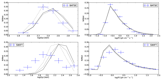
Figure 1.: Top left: peak energy distribution observed by BATSE. Bottom left: peak energy distribution observed by SWIFT. Top right: peak flux distribution observed by BATSE. Bottom left: peak flux distribution observed by SWIFT. The lines represent results for our simulation with values of $Z_{\text{max}}$: 1 (solid), 0.01 (dashed) and 0.006 (dotted)

References

- Artale et al. (2011) Artale M. C., Pellizza L. J., Tissera P. B., 2011, MNRAS, 415, 3417
- Band et al. (1993) Band D., et al., 1993, ApJ, 413, 281
- Band (2006) Band D. L., 2006, ApJ, 644, 378
- Chabrier (2003) Chabrier G., 2003, PASP, 115, 763
- Chisari et al. (2010) Chisari N. E., Tissera P. B., Pellizza L. J., 2010, MNRAS, 408, 647
- da Silva et al. (2012) da Silva R. L., Fumagalli M., Krumholz M., 2012, ApJ, 745, 145
- Daigne et al. (2006) Daigne F., Rossi E. M., Mochkovitch R., 2006, MNRAS, 372, 1034
- Le Floc’h et al. (2003) Le Floc’h E., et al., 2003, A&A, 400, 499
- Li et al. (2008) Li A., et al., 2008, ApJ, 685, 1046
- Nuza et al. (2007) Nuza S. E., et al., 2007, MNRAS, 375, 665
- Salvaterra & Chincarini (2007) Salvaterra R., Chincarini G., 2007, ApJ Letters, 656, L49
- Savaglio et al. (2009) Savaglio S., Glazebrook K., Le Borgne D., 2009, ApJ, 691, 182
- Scannapieco et al. (2006) Scannapieco C., et al., 2006, MNRAS, 371, 1125
- Stern et al. (2001) Stern B. E., et al., 2001, ApJ, 563, 80