Variational approach for spatial point process intensity estimation

Abstract

We introduce a new variational estimator for the intensity function of an inhomogeneous spatial point process with points in the $d$-dimensional Euclidean space and observed within a bounded region. The variational estimator applies in a simple and general setting when the intensity function is assumed to be of log-linear form $\beta+{\theta}^{\top}z(u)$ where $z$ is a spatial covariate function and the focus is on estimating ${\theta}$. The variational estimator is very simple to implement and quicker than alternative estimation procedures. We establish its strong consistency and asymptotic normality. We also discuss its finite-sample properties in comparison with the maximum first order composite likelihood estimator when considering various inhomogeneous spatial point process models and dimensions as well as settings were $z$ is completely or only partially known.

and

1 Introduction

Intensity estimation for spatial point processes is of fundamental importance in many applications, see, for example, Diggle [10], Møller and Waagepetersen [28], Illian et al. [21], Baddeley [2], and Diggle [11]. While maximum likelihood and Bayesian methods are feasible for parametric Poisson point process models (Berman and Turner [6]), computationally intensive Markov chain Monte Carlo methods are needed otherwise (Møller and Waagepetersen [27]). The Poisson likelihood has been used for intensity estimation in non-Poisson models (Schoenberg [31], Guan and Shen [16]) where it can be viewed as a composite likelihood based on the intensity function (Møller and Waagepetersen [28] and Waagepetersen [34]); we refer to this as a “first order composite likelihood”. For Cox and Poisson cluster point processes, which form major classes of point process models for clustering or aggregation (Stoyan, Kendall and Mecke [32]), the first and second order moment properties as expressed by the intensity function $\rho$ and pair correlation function $g$ are often of an explicit form, and this has led to the development of estimation procedures based on combinations of first and second order composite likelihoods and minimum contrast estimation procedures (Guan [13], Møller and Waagepetersen [28], Waagepetersen [34]) and to refinements of such methods (Guan and Shen [16], Guan, Jalilian and Waagepetersen [14]). For Gibbs point processes, which form a major class of point process models for repulsiveness, the (Papangelou) conditional intensity is of explicit form and has been used for developing maximum pseudo-likelihood estimators (Besag [7], Jensen and Møller [24], Baddeley and Turner [4]) and variational estimators (Baddeley and Dereudre [3]). However, in general for Gibbs point processes, the moment properties are not expressible in closed form and it is therefore hard to estimate the intensity function.

The present paper considers a new variational estimator for the intensity function of a spatial point process $\mathbf{X}$, with points in the $d$-dimensional Euclidean space $\mathbb{R}^{d}$ and observed within a bounded region $W\subset\mathbb{R}^{d}$. It is to some extent derived along similar lines as the variational estimator based on the conditional intensity (Baddeley and Dereudre [3]), which in turn is a counterpart of the variational estimator for Markov random fields (Almeida and Gidas [1]). However, our variational estimator applies in a much simpler and general setting. In analogy with the exponential form of the conditional intensity considered in Baddeley and Dereudre [3], we assume that $\mathbf{X}$ has a log-linear intensity function

$$\rho(u)=\exp\bigl{(}\beta+{\theta}^{\top}z(u)\bigr{)},\qquad u\in\mathbb{R}^{d}.$$ (1)

Here $\beta$ is a real parameter, ${\theta}$ is a real $p$-dimensional parameter and ${\theta}^{\top}$ is its transpose, $z$ is a real $p$-dimensional function defined on $\mathbb{R}^{d}$ and referred to as the covariate function, and we view ${\theta}$ and $z(u)$ as column vectors. A log-linear intensity function is often assumed for Poisson point processes (where it is the canonical link) and for Cox processes (see Møller and Waagepetersen [28] and the references therein), while for Gibbs point process models it is hard to exhibit a model with intensity function of the log-linear form. Further details are given in Sections 2–3.

As the variational estimator in Baddeley and Dereudre [3], our variational estimator concerns $\theta$, while $\beta$ is treated as a nuisance parameter which is not estimated. Our variational estimator is simple to implement, it requires only the computation of the solution of a system of $p$ linear equations involving certain sums over the points of $\mathbf{X}$ falling in $W$, and it is quicker to use than the other estimation methods mentioned above. Moreover, our variational estimator is expressible in closed form while the maximum likelihood estimator for the Poisson likelihood and the maximum first order composite likelihood estimator for non-Poisson models are not expressible in closed form and the profile likelihood for $\theta$ involves the computation (or approximation) of $d(1+p/2)(p+1)$ integrals. On the one hand, as for the approach based on first order composite likelihoods, an advantage of our variational estimator is its flexibility, since apart from (1) and a few mild assumptions on $z$, we do not make any further assumptions. In particular, we do not require that $\mathbf{X}$ is a grand canonical Gibbs process as assumed in Baddeley and Dereudre [3]. On the other hand, a possible disadvantage of our variational approach is a loss in efficiency, since we do not take into account spatial correlation, for example, through the modelling of the pair correlation function as in Guan and Shen [16] and Guan, Jalilian and Waagepetersen [14], or interaction, for example, through the modelling of the conditional intensity function as in Baddeley and Dereudre [3].

The paper is organized as follows. Section 2 presents our general setting. Section 3 specifies our variational estimator, establishes its asymptotic properties, and discusses the conditions we impose. Section 4 reports on a simulation study of the finite-sample properties of our variational estimator and the maximum first order composite likelihood estimator for various inhomogeneous spatial point process models in the planar case $d=2$ as well as higher dimensions and when $z$ is known on an observation window as well as when $z$ is known only on a finite set of locations. The technical proofs of our results are deferred to Appendix A. Finally, Appendix B illustrates the simplicity of our variational estimator and the flexibility of the conditions given in Section 3.

2 Preliminaries

This section introduces the assumptions and notation used throughout this paper.

Let $W\subset\mathbb{R}^{d}$ be a compact set of positive Lebesgue measure $|W|$. It will play the role of an observation window. Without any danger of confusion, we also use the notation $|A|$ for the cardinality of a countable set $A$, and $|u|=\max\{|u_{i}|\colon\ i=1,\ldots,d\}$ for the maximum norm of a point $u=(u_{1},\ldots,u_{d})\in\mathbb{R}^{d}$. Further, we let $\|u\|$ denote the Euclidean norm for a point $u\in\mathbb{R}^{d}$, and $\|A\|={\sup_{\|u\|=1}}|Au|$ the supremum norm for a square matrix $A$, that is, its numerically largest (right) eigenvalue. Moreover, for any real $p$-dimensional function $k$ defined on $\mathbb{R}^{d}$, we let

$$\|k\|_{\infty}=\sup_{u\in\mathbb{R}^{d}}\bigl{\|}k(u)\bigr{\|}.$$ (2)

Let $\mathbf{X}$ be a spatial point process on $\mathbb{R}^{d}$, which we view as a random locally finite subset of $\mathbb{R}^{d}$. Let $\mathbf{X}_{W}=\mathbf{X}\cap W$. Then the number of points in $\mathbf{X}_{W}$ is finite; we denote this number by $N(W)=n(\mathbf{X}_{W})=|\mathbf{X}_{W}|$; and a realization of $\mathbf{X}_{W}$ is of the form $\mathbf{x}=\{x_{1},\ldots,x_{n}\}\subset W$, where $n=n(\mathbf{x})$ and $0\leq n<\infty$. If $n=0$, then $\mathbf{x}=\varnothing$ is the empty point pattern in $W$. For further background material and measure theoretical details on spatial point process, see, for example, Daley and Vere-Jones [9] and Møller and Waagepetersen [27].

We assume that $\mathbf{X}$ has a locally integrable intensity function $\rho$. By Campbell’s theorem (see, e.g., Møller and Waagepetersen [27]), for any real Borel function $k$ defined on $\mathbb{R}^{d}$ such that $k\rho$ is absolutely integrable (with respect to the Lebesgue measure on $\mathbb{R}^{d}$),

$$\mathrm{E}\sum_{u\in\mathbf{X}}k(u)=\int k(u)\rho(u)\,\mathrm{d}u.$$ (3)

Furthermore, for any integer $n\geq 1$, $\mathbf{X}$ is said to have an $n$th order product density $\rho^{(n)}$ if this is a non-negative Borel function on $\mathbb{R}^{dn}$ such that for all non-negative Borel functions $k$ defined on $\mathbb{R}^{dn}$,

$$\mathrm{E}\sum^{\neq}_{u_{1},\ldots,u_{n}\in\mathbf{X}}k(u_{1},\ldots,u_{n})=\int\cdots\int k(u_{1},\ldots,u_{n})\rho^{(n)}(u_{1},\ldots,u_{n})\,\mathrm{d}u_{1}\cdots\mathrm{d}u_{n},$$ (4)

where the $\neq$ over the summation sign means that $u_{1},\ldots,u_{n}$ are pairwise distinct. Note that $\rho=\rho^{(1)}$.

Throughout this paper except in Section 3.1, we assume that $\rho$ is of the log-linear form (1), where we view ${\theta}$ and $z(u)$ as $p$-dimensional column vectors.

As for vectors, transposition of a matrix $A$ is denoted $A^{\top}$. For convenience, we, for example, write $(\beta,{\theta})$ when we more precisely mean the $(p+1)$-dimensional column vector $(\beta,{\theta}^{\top})^{\top}$. If $A$ is a square matrix, we write $A\geq 0$ if $A$ is positive semi-definite, and $A>0$ if $A$ is (strictly) positive definite. When $A$ and $B$ are square matrices of the same size, we write $A\geq B$ if $A-B\geq 0$.

For $k=0,1,\ldots\,$, denote $\mathcal{C}_{d,p}^{k}$ the class of $k$-times continuous differentiable real $p$-dimensional functions defined on $\mathbb{R}^{d}$. For $h\in\mathcal{C}_{d,1}^{1}$, denote its gradient

$$\nabla h(u)=\biggl{(}\frac{\partial h}{\partial u_{1}}(u),\ldots,\frac{\partial h}{\partial u_{d}}(u)\biggr{)}^{\top},\qquad u=(u_{1},\ldots,u_{d})^{\top}\in\mathbb{R}^{d}$$

and define the divergence operator $\operatorname{div}$ on $\mathcal{C}_{d,1}^{1}$ by

$$\operatorname{div}h(u)=\frac{\partial h}{\partial u_{1}}(u)+\cdots+\frac{\partial h}{\partial u_{d}}(u),\qquad u=(u_{1},\ldots,u_{d})^{\top}\in\mathbb{R}^{d}.$$

Furthermore, for $h=(h_{1},\ldots,h_{p})^{\top}\in\mathcal{C}_{d,p}^{1}$, define the divergence operator $\operatorname{div}$ on $\mathcal{C}_{d,p}^{1}$ by

$$\operatorname{div}h(u)=\bigl{(}\operatorname{div}h_{1}(u),\ldots,\operatorname{div}h_{p}(u)\bigr{)}^{\top},\qquad u\in\mathbb{R}^{d}.$$

If $z\in\mathcal{C}_{d,p}^{1}$, then by (1)

$$\operatorname{div}\log\rho(u)={\theta}^{\top}\operatorname{div}z(u)=\operatorname{div}z(u)^{\top}{\theta},\qquad u\in\mathbb{R}^{d}.$$ (5)

Finally, we recall the classical definition of mixing coefficients (see, e.g., Politis, Paparoditis and Romano [29]): for $j,k\in\mathbb{N}\cup\{\infty\}$ and $m\geq 1$, define

$$\alpha_{j,k}(m) = \sup\bigl{\{}\bigl{|}P(A\cap B)-P(A)P(B)\bigr{|}\colon\ A\in\mathcal{F}(\Lambda_{1}),B\in\mathcal{F}(\Lambda_{2}),$$

$$\hskip 20.6pt\Lambda_{1}\in\mathcal{B}\bigl{(}\mathbb{R}^{d}\bigr{)},\Lambda_{2}\in\mathcal{B}\bigl{(}\mathbb{R}^{d}\bigr{)},|\Lambda_{1}|\leq j,|\Lambda_{2}|\leq k,d(\Lambda_{1},\Lambda_{2})\geq m\bigr{\}},$$

where $\mathcal{F}(\Lambda_{i})$ is the $\sigma$-algebra generated by $X\cap\Lambda_{i}$, $i=1,2$, $d(\Lambda_{1},\Lambda_{2})$ is the minimal distance between the sets $\Lambda_{1}$ and $\Lambda_{2}$, and $\mathcal{B}(\mathbb{R}^{d})$ denotes the class of Borel sets in $\mathbb{R}^{d}$.

3 The variational estimator

Section 3.1 establishes an identity which together with (5) is used in Section 3.2 for deriving an unbiased estimating equation which only involves ${\theta}$, the parameter of interest, and from which our variational estimator is derived. Section 3.3 discusses the asymptotic properties of the variational estimator.

3.1 Basic identities

This section establishes some basic identities for a spatial point process $\mathbf{X}$ defined on $\mathbb{R}^{d}$ and having a locally integrable intensity function $\rho$ which is not necessarily of the log-linear form (1). The results will be used later when defining our variational estimator.

Consider a real Borel function $h$ defined on $\mathbb{R}^{d}$ and let $f(u)=\rho(u)|h(u)|$. For $n=1,2,\ldots\,$, let $E_{n}^{d}=[-n,n]^{d}$ and

$$\mu_{n}(f)=\max\bigl{\{}\mu_{n,j}(f)\colon\ j=1,\ldots,d\bigr{\}}$$

with

$$\mu_{n,j}(f) = \int_{E_{n}^{d-1}}f(u_{1},\ldots,u_{j-1},-n,u_{j+1},\ldots,u_{d})\,\mathrm{d}u_{1}\cdots\mathrm{d}u_{j-1}\,\mathrm{d}u_{j+1}\cdots\mathrm{d}u_{n}$$

$${}+\int_{E_{n}^{d-1}}f(u_{1},\ldots,u_{j-1},n,u_{j+1},\ldots,u_{d})\,\mathrm{d}u_{1}\cdots\mathrm{d}u_{j-1}\,\mathrm{d}u_{j+1}\cdots\mathrm{d}u_{n}$$

provided the integrals exist. Note that $\mu_{n}(f)$ depends only on the behaviour of $f$ on the boundary of $E_{n}^{d}$.

Proposition 3.1

Suppose that $h,\rho\in\mathcal{C}^{1}_{d,1}$ such that $\lim_{n\rightarrow\infty}\mu_{n}(\rho|h|)=0$ and for $j=1,\ldots,d$, the function $h(u)\,\partial\rho(u)/\partial u_{j}$ is absolutely integrable. Then the following relations hold where the mean values exist and are finite:

$$\mathrm{E}\sum_{u\in\mathbf{X}}h(u)\nabla\log\bigl{(}\rho(u)\bigr{)}=-\mathrm{E}\sum_{u\in\mathbf{X}}\nabla h(u)$$ (6)

and

$$\mathrm{E}\sum_{u\in\mathbf{X}}h(u)\operatorname{div}\log\bigl{(}\rho(u)\bigr{)}=-\mathrm{E}\sum_{u\in\mathbf{X}}\operatorname{div}h(u).$$ (7)

[Proof.] For $j=1,\ldots,d$ and $u=(u_{1},\ldots,u_{d})^{\top}\in\mathbb{R}^{d}$, Campbell’s theorem (3) and the assumption that $h(u)\,\partial\rho(u)/\partial u_{j}$ is absolutely integrable imply that

$$\mathrm{E}\biggl{(}\sum_{u\in\mathbf{X}}h(u)\nabla\log\bigl{(}\rho(u)\bigr{)}\biggr{)}_{j}=\int h(u)\,\frac{\partial\rho}{\partial u_{j}}(u)\,\mathrm{d}u$$

exist. Thereby,

$$\mathrm{E}\biggl{(}\sum_{u\in\mathbf{X}}h(u)\nabla\log\bigl{(}\rho(u)\bigr{)}\biggr{)}_{j}$$

$$\quad=\lim_{n\to\infty}\int_{E_{n}^{d}}h(u)\,\frac{\partial\rho}{\partial u_{j}}(u)\,\mathrm{d}u$$

$$\quad=\lim_{n\to\infty}\int_{E_{n}^{d-1}}\biggl{(}\bigl{[}\rho(u)h(u)\bigr{]}_{u_{j}=-n}^{u_{j}=n}-\int_{-n}^{n}\rho(u)\,\frac{\partial h}{\partial u_{j}}(u)\,\mathrm{d}u_{j}\biggr{)}\,\mathrm{d}u_{1}\cdots\mathrm{d}u_{j-1}\,\mathrm{d}u_{j+1}\cdots\mathrm{d}u_{n}$$

$$\quad=-\lim_{n\to\infty}\int_{E_{n}^{d}}\frac{\partial h}{\partial u_{j}}(u)\rho(u)\,\mathrm{d}u,$$

where the first identity follows from the dominated convergence theorem, the second from Fubini’s theorem and integration by parts, and the third from Fubini’s theorem and the assumption that $\lim_{n\rightarrow\infty}\mu_{n}(\rho|h|)=0$, since

$$\biggl{|}\int_{E_{n}^{d-1}}\bigl{[}\rho(u)h(u)\bigr{]}_{u_{j}=-n}^{u_{j}=n}\biggr{|}\leq\mu_{n,j}\bigl{(}\rho|h|\bigr{)}\leq\mu_{n}\bigl{(}\rho|h|\bigr{)}.$$

Hence, using first the dominated convergence theorem and second Campbell’s theorem,

$$\mathrm{E}\biggl{(}\sum_{u\in\mathbf{X}}h(u)\nabla\log\bigl{(}\rho(u)\bigr{)}\biggr{)}_{j}=-\int\frac{\partial h}{\partial u_{j}}(u)\rho(u)\,\mathrm{d}u=-\mathrm{E}\biggl{(}\sum_{u\in\mathbf{X}}\nabla h(u)\biggr{)}_{j}$$

whereby (6) is verified and the mean values in (6) are seen to exist and are finite. Finally, (6) implies (7) where the mean values exist and are finite.

Proposition 3.1 becomes useful when $\rho$ is of the log-linear form (1): if we omit the expectation signs in (6)–(10), we obtain unbiased estimating equations, where (6) gives a linear system of $p$ vectorial equation in dimension $d$, while (10) gives a linear system of $p$ one-dimensional equations for the estimation of the $p$-dimensional parameter $\theta$; the latter system is simply obtained by summing over the $d$ equations in each vectorial equation. A similar reduction of equations is obtained in Baddeley and Dereudre [3].

The conditions and the last result in Proposition 3.1 simplify as follows when $h$ vanishes outside $W$.

Corollary 3.2

Suppose that $h,\rho\in\mathcal{C}^{1}_{d,1}$ such that $h(u)=0$ whenever $u\notin W$. Then

$$\mathrm{E}\sum_{u\in\mathbf{X}_{W}}h(u)\operatorname{div}\log\bigl{(}\rho(u)\bigr{)}=-\mathrm{E}\sum_{u\in\mathbf{X}_{W}}\operatorname{div}h(u).$$ (8)

3.2 The variational estimator

Henceforth we consider the case of the log-linear intensity function (1), assuming that the parameter space for $(\beta,{\theta})$ is $\mathbb{R}\times\mathbb{R}^{p}$. We specify below our variational estimator in terms of a $p$-dimensional real test function

$$h=(h_{1},\ldots,h_{p})^{\top}$$

defined on $\mathbb{R}^{d}$. The test function is required not to depend on $(\beta,{\theta})$ and to satisfy certain smoothness conditions. The specific choice of test functions is discussed at the end of Section 3.2.2.

In the present section, to stress that the expectation of a functional $f$ of $\mathbf{X}$ depends on $(\beta,{\theta})$, we write this as $\mathrm{E}_{\beta,{\theta}}f(\mathbf{X})$. Furthermore, define the $p\times p$ matrix

$$A(\mathbf{X}_{W})=\sum_{u\in\mathbf{X}_{W}}h(u)\operatorname{div}z(u)^{\top}$$

and the $p$-dimensional column vector

$$b(\mathbf{X}_{W})=\sum_{u\in\mathbf{X}_{W}}\operatorname{div}h(u).$$

3.2.1 Estimating equation and definition of the variational estimator

We consider first the case where the test function $h$ vanishes outside $W$.

Corollary 3.3

Suppose that $h,z\in\mathcal{C}^{1}_{d,p}$ such that

$$h(u)=0 u\notin W$$      whenever . (9)

Then, for any $(\beta,{\theta})\in\mathbb{R}\times\mathbb{R}^{p}$,

$$\mathrm{E}_{\beta,{\theta}}A(\mathbf{X}_{W}){\theta}=-\mathrm{E}_{\beta,{\theta}}b(\mathbf{X}_{W}).$$ (10)

[Proof.] The conditions of Corollary 3.2 are easily seen to be satisfied. Hence combining (5) and (8) we obtain (10).

Several remarks are in order.

Note that (10) is a linear system of $p$ equations for the $p$-dimensional parameter $\theta$. Under the conditions in Corollary 3.3, (10) leads to the unbiased estimating equation

$$A(\mathbf{X}_{W})\theta=-b(\mathbf{X}_{W}).$$ (11)

Theorem 3.5 below establishes that under certain conditions, where we do not necessarily require $h$ to vanish outside $W$, (11) is an asymptotically unbiased estimating equation as $W$ extends to $\mathbb{R}^{d}$.

In the sequel we therefore do not necessarily assume (9). For instance, when $\operatorname{div}z(u)$ does not vanish outside $W$, we may consider either $h(u)=\operatorname{div}z(u)$ or $h(u)=\eta_{W}(u)\operatorname{div}z(u)$, where $\eta_{W}$ is a smooth function which vanishes outside $W$. In the latter case, (11) is an unbiased estimating equation, while in the former case it is an asymptotically unbiased estimating equation (under the conditions imposed in Theorem 3.5).

When (11) is an (asymptotically) unbiased estimating equation and $A(\mathbf{X}_{W})$ is invertible, we define the variational estimator by

$$\widehat{\theta}=-A(\mathbf{X}_{W})^{-1}b(\mathbf{X}_{W}).$$ (12)

Theorem 3.5 below establishes under certain conditions the invertibility of $A(\mathbf{X}_{W})$ and the strong consistency and asymptotic normality of $\widehat{\theta}$ as $W$ extends to $\mathbb{R}^{d}$.

Finally, if $h$ is allowed to depend on $\theta$, (11) still provides an unbiased estimating equation but the closed form expression (12) only applies when $h$ is not depending on $\theta$ (as assumed in this paper).

3.2.2 Choice of test function

The choice of test function should take into consideration the conditions introduced later in Section 3.3.1. The test functions below are defined in terms of the covariate function so that it is possible to check these conditions as discussed in Section 3.3.2.

Interesting choices of the test function include:

• $h(u)=\operatorname{div}z(u)$ and the corresponding modification $h(u)=\eta_{W}(u)\operatorname{div}z(u)$,

• $h(u)=z(u)$ and the corresponding modification $h(u)=\eta_{W}(u)z(u)$.

In the first case, $A(\mathbf{X}_{W})$ becomes a covariance matrix. For example, if $h(u)=\operatorname{div}z(u)$, then

$$A(\mathbf{X}_{W})=\sum_{u\in\mathbf{X}_{W}}\operatorname{div}z(u)\operatorname{div}z(u)^{\top}$$

is invertible if and only if $A(\mathbf{X}_{W})>0$, meaning that if $\mathbf{X}_{W}=\{x_{1},\ldots,x_{n}\}$ is observed, then the $p\times n$ matrix with columns $\operatorname{div}z(x_{1}),\ldots,\operatorname{div}z(x_{n})$ has rank $p$. In the latter case, $A(\mathbf{X}_{W})$ is in general not symmetric and we avoid the calculation of $\operatorname{div}\operatorname{div}z(u)$.

3.2.3 Choice of smoothing function

We let henceforth the smoothing function $\eta_{W}$ depend on a user-specified parameter $\varepsilon>0$ and define it as the convolution

$$\eta_{W}(u)=\chi_{W_{\ominus\varepsilon}}*\varphi_{\varepsilon}(u)=\int\mathbf{1}(u-v\in W_{\ominus\varepsilon})\varphi_{\varepsilon}(v)\,\mathrm{d}v,\qquad u\in\mathbb{R}^{d},$$ (13)

where the notation means the following:

$${W}_{\ominus\varepsilon}=\bigl{\{}u\in W\colon\ b(u,\varepsilon)\subseteq W\bigr{\}}$$

is the observation window eroded by the $d$-dimensional closed ball $b(u,\varepsilon)$ centered at $u$ and with radius $\varepsilon$; $\chi_{W_{\ominus\varepsilon}}(\cdot)=\mathbf{1}(\cdot\in W_{\ominus\varepsilon})$ is the indicator function on $W_{\ominus\varepsilon}$; and

$$\varphi_{\varepsilon}(u)=\varepsilon^{-d}\varphi(u/\varepsilon),\qquad u\in\mathbb{R}^{d},$$

where

$$\varphi(u)=c\exp\biggl{(}{-\frac{1}{1-\|u\|^{2}}}\biggr{)}\mathbf{1}\bigl{(}\|u\|\leq 1\bigr{)},\qquad u\in\mathbb{R}^{d},$$

where $c$ is a normalizing constant such that $\varphi$ is a density function ($c\approx 2.143$ when $d=2$). Figure 1 shows the function $\eta_{W}$ and its divergence when $W=[-1,1]^{2}$, $\varepsilon=0.2$, and $\varepsilon=0.4$. The construction (13) is quite standard in distribution theory when functions are regularized and it can be found, though in a slightly different form, in Hörmander ([19], Theorem 1.4.1, page 25).

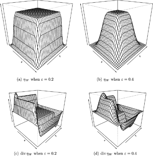
Figure 1: Plots of the functions $\eta_{W}=\chi_{W}*\varphi_{\varepsilon}$ and $\operatorname{div}\eta_{W}$ when $W=[-1,1]^{2}$ and $\varepsilon=0.2,0.4$.

It is easily checked that $\varphi_{\varepsilon}\in\mathcal{C}^{\infty}_{d,1}$, and so $\eta_{W}\in\mathcal{C}^{\infty}_{d,1}$. Note that

$$0\leq\eta_{W}\leq 1,\qquad\eta_{W}(u)=1\qquad\mbox{if $u\in W_{\ominus 2\varepsilon}$},\qquad\eta_{W}(u)=0\qquad\mbox{if $u\notin W$}.$$ (14)

The following lemma states some properties for test functions of the modified form $h(u)=\eta_{W}(u)k(u)$, where we let $\kappa=\int_{\mathcal{B}(0,1)}|{\operatorname{div}\varphi(v)}|\,\mathrm{d}v$; if $d=2$ then $\kappa\approx 1.256$.

Lemma 3.4

Let $k\in\mathcal{C}^{1}_{d,p}$ and $h(u)=\eta_{W}(u)k(u)$ where $\eta_{W}$ is given by (13). Then $h\in\mathcal{C}^{1}_{d,p}$ and its support is included in $W$. Further, $h$ respective $\operatorname{div}h$ agrees with $k$ respective $\operatorname{div}k$ on ${W}_{\ominus 2\varepsilon}$. Moreover, for any $u\in{W}$,

$$\bigl{\|}h(u)\bigr{\|}\leq\bigl{\|}k(u)\bigr{\|},\qquad\bigl{\|}\operatorname{div}h(u)-\operatorname{div}k(u)\bigr{\|}\leq\bigl{\|}\operatorname{div}k(u)\bigr{\|}+\bigl{\|}k(u)\bigr{\|}{\kappa}/{\varepsilon}.$$ (15)

[Proof.] We have $h\in\mathcal{C}^{1}_{d,p}$ since $k\in\mathcal{C}^{1}_{d,p}$ and $\eta_{W}\in\mathcal{C}^{\infty}_{d,1}$, and the support of $h$ is included in $W$ since $\eta_{W}(u)=0$ if $u\notin W$. From the last two statements of (14), we obtain that $\operatorname{div}h(u)$ agrees with $\operatorname{div}k(u)$ on $W_{\ominus 2\varepsilon}$. The first inequality in (15) follows immediately from the definition of $h$, since $\|h(u)\|=\|\eta_{W}(u)k(u)\|\leq\|k(u)\|$. Recall that $(f*g)^{\prime}=f*g^{\prime}$ if $g\in C^{1}_{d,p}$ has compact support and $f$ is Lebesgue integrable on $\mathbb{R}^{d}$, where in our case we let $f=\chi_{W_{\ominus\varepsilon}}$ and $g=\varphi_{\varepsilon}$. Therefore and since $\operatorname{div}\varphi_{\varepsilon}=(\operatorname{div}\varphi)/\varepsilon\in\mathcal{C}^{\infty}_{d,1}$, for any $u\in W$, we have

$$\operatorname{div}h(u) = \eta_{W}(u)\operatorname{div}k(u)+k(u)(\chi_{{W}_{\ominus\varepsilon}}*\operatorname{div}\varphi_{\varepsilon})(u)$$

$$= \eta_{W}(u)\operatorname{div}k(u)+\frac{1}{\varepsilon}k(u)(\chi_{W_{\ominus\varepsilon}}*\operatorname{div}\varphi)(u).$$

Thereby, the second inequality in (15) follows from a straightforward calculation using again the fact that $\eta_{W}(u)\leq 1$.

3.3 Asymptotic results

In this section, we present asymptotic results for the variational estimator when considering a sequence of observation windows $W=W_{n}$, $n=1,2,\ldots\,$, which expands to $\mathbb{R}^{d}$ as $n\to\infty$, and a corresponding sequence of test functions $h=h^{(n)}$, $n=1,2,\ldots\,$. Corresponding to the two cases of test functions considered in Section 3.2.1, we consider the following two cases:

1. either $h^{(n)}=k$ does not depend on $n$,

2. or $h^{(n)}(u)=\eta_{W_{n}}(u)k(u)$, where $\eta_{W_{n}}$ is given by (13).

3.3.1 Conditions

Our asymptotic results require the following conditions.

We restrict attention to the spatial case $d\geq 2$ (this is mainly for technical reasons as explained in Section 3.3.3). We suppress in the notation that the intensity $\rho$ and the higher order product densities $\rho^{(2)},\rho^{(3)},\ldots$ depend on the “true parameters” $(\beta,\theta)$. Let

$$S_{n}=\int_{W_{n}}h^{(n)}(u)\operatorname{div}z(u)^{\top}\rho(u)\,\mathrm{d}u$$ (16)

and

$$\Sigma_{n}=\int_{W_{n}}f^{(n)}_{\theta}(u)f^{(n)}_{\theta}(u)^{\top}\rho(u)\,\mathrm{d}u+\int_{W_{n}^{2}}f^{(n)}_{\theta}(u_{1})f^{(n)}_{\theta}(u_{2})^{\top}Q_{2}(u_{1},u_{2})\,\mathrm{d}u_{1}\,\mathrm{d}u_{2},$$ (17)

where $Q_{2}(u_{1},u_{2})=\rho^{(2)}(u_{1},u_{2})-\rho(u_{1})\rho(u_{2})$ (assuming $\rho^{(2)}$ exists) and

$$f_{\theta}^{(n)}(u)=h^{(n)}(u)\operatorname{div}z(u)^{\top}\theta+\operatorname{div}h^{(n)}(u),\qquad u\in\mathbb{R}^{d}.$$

It will follow from the proof of Theorem 3.5 below that under the conditions (i)–(vi) stated below, with probability one, the integrals in (16)–(17) exist and are finite for all sufficiently large $n$.

We impose the following conditions, where $o$ denotes the origin of $\mathbb{R}^{d}$:

1. [(iii)]

2. For every $n\geq 1$, $W_{n}=nA=\{na\colon\ a\in A\}$, where $A\subset\mathbb{R}^{d}$ is convex, compact, and contains $o$ in its interior.

3. The test functions $h^{(n)}$, $n=1,2,\ldots\,$, and the covariate function $z$ are elements of $\mathcal{C}^{1}_{d,p}$, and satisfy for some constant $K>0$,

   $$\|z\|_{\infty} \leq K,\qquad\|{\operatorname{div}z}\|_{\infty}\leq K,$$

   $$\sup_{n\geq 1}\bigl{\|}h^{(n)}\bigr{\|}_{\infty} \leq K,\qquad\sup_{n\geq 1}\bigl{\|}\operatorname{div}h^{(n)}\bigr{\|}_{\infty}\leq K.$$

4. There exists a $p\times p$ matrix $I_{0}$ such that for all sufficiently large $n$, we have $S_{n}/|W_{n}|\geq I_{0}>0$.

5. There exists an integer $\delta\geq 1$ such that for $k=1,\ldots,2+\delta$, the product density $\rho^{(k)}$ exists and $\rho^{(k)}\leq K^{\prime}$, where $K^{\prime}<\infty$ is a constant.

6. For the strong mixing coefficients (Section 2), we assume that there exists some $\nu>d(2+\delta)/\delta$ such that $a_{2,\infty}(m)=\mathcal{O}(m^{-\nu})$.

7. The second order product density $\rho^{(2)}$ exists, and there exists a $p\times p$ matrix $I^{\prime}_{0}$ such that for all sufficiently large $n$, $\Sigma_{n}/|W_{n}|\geq I^{\prime}_{0}>0$.

3.3.2 Discussion of the conditions

Some comments on conditions (i)–(vi) are in order.

In general in applications, the observation window has a non-empty interior. In (i), the assumption that $A$ contains $o$ in its interior can be made without loss of generality; if instead $u$ was an interior point of $A$, then (i) could be modified to that any ball with centre $u$ and radius $r>0$ is contained in $W_{n}=nA$ for all sufficiently large $n$. We could also modify (i) to the case where $|A|>0$ and as $n\rightarrow\infty$ the limit of $W_{n}=nA$ exists and is given by $W_{\infty}$; then in ((ii)) we should redefine $\|\cdot\|_{\infty}=\sup_{u\in\mathbb{R}^{d}}\|k(u)\|$ (i.e., as defined in (2)) by $\|\cdot\|_{\infty}=\sup_{u\in W_{\infty}}\|k(u)\|$. For either case, Theorem 3.5 in Section 3.3.3 will remain true, as the proof of the theorem (given in Appendix A) can easily be modified to cover these cases.

In (ii), for both cases of (A) and (B) and for $k(u)=\operatorname{div}z(u)$, ((ii)) simplifies to

$$\|z\|_{\infty}\leq K,\qquad\|{\operatorname{div}z}\|_{\infty}\leq K,\qquad\|{\operatorname{div}\operatorname{div}z}\|_{\infty}\leq K.$$ (19)

This follows immediately for the case (A), since then $h^{(n)}=h$ does not depend on $n$, while in the case (B) where $h^{(n)}(u)=\eta_{W_{n}}(u)k(u)$, Lemma 3.4 implies the equivalence of ((ii)) and (19).

Note that in (ii) we do not require that $h^{(n)}$ vanishes outside $W_{n}$. Thus, in connection with the unbiasedness result in Corollary 3.3, one of the difficulties to prove Theorem 3.5 below will be to “approximate” $h^{(n)}$ by a function with support $W_{n}$, as detailed in Appendix A.

Conditions (iii) and (vi) are spatial average assumptions like when establishing asymptotic normality of ordinary least square estimators for linear models. These conditions must be checked for each choice of covariate function, since they depend strongly on $z$. Note that under condition (ii), for any $u\in\mathbb{R}^{d}$, $\rho(u)\geq\exp(\beta-\|\theta\|_{\infty}\|z\|_{\infty})=c>0$. Therefore, condition (iii) is satisfied if $h^{(n)}(u)\operatorname{div}z(u)^{\top}\geq 0$ for any $u$ and if $|W_{n}|^{-1}\int_{W_{n}}h^{(n)}(u)\operatorname{div}z(u)^{\top}\,\mathrm{d}u\geq I_{0}$ for all sufficiently large $n$. In addition, if $Q_{2}(u_{1},u_{2})\geq 0$ for any $u_{1},u_{2}\in\mathbb{R}^{d}$ (this is discussed above for specific point process models), then condition (vi) is satisfied if $|W_{n}|^{-1}\int_{W_{n}}f^{(n)}(u)f^{(n)}(u)^{\top}\,\mathrm{d}u\geq I_{0}^{\prime}$ for all sufficiently large $n$.

Condition (iv) is not very restrictive. It is fulfilled for any Gibbs point process with a Papangelou conditional intensity which is uniformly bounded from above (the so-called local stability condition, see, e.g., Møller and Waagepetersen [27]), and also for a log-Gaussian Cox process where the mean and covariance functions of the underlying Gaussian process are uniformly bounded from above (see Møller, Syversveen and Waagepetersen [26] and Møller and Waagepetersen [28]). Note that the larger we can choose $\delta$, the weaker becomes condition (v).

Condition (v) combined with (iv) is also considered in Waagepetersen and Guan [33], and (iv)–(v) are inspired by a central limit theorem obtained first by Bolthausen [8] and later extended to non-stationary random fields in Guyon [17] and to triangular arrays of non-stationary random fields (which is the requirement of our setting) in Karácsony [25]. We underline that we turned to a central limit theorem using mixing conditions instead of one using martingale type assumptions (e.g., Jensen and Künsch [23]) since for most of models considered in this paper (in particular the two Cox processes discussed below) the “martingale” type assumption is not satisfied. Such an assumption is more devoted to Gibbs point processes.

Other papers dealing with asymptotics for estimators based on estimating equations for spatial point processes (e.g., Guan [13], Guan and Loh [15], Guan and Shen [16], Guan, Jalilian and Waagepetersen [14], Prokešová and Jensen [30]) are assuming mixing properties expressed in terms of a different definition of mixing coefficient (see, e.g., Equations (5.2)–(5.3) in Prokešová and Jensen [30]). The mixing conditions in these papers are related to a central limit theorem by Ibragimov and Linnik [20] obtained using blocking techniques, and the mixing conditions may seem slightly less restrictive than our condition (v). However, rather than our condition (iv), it is assumed in the papers that the first four reduced cumulants exist and have finite total variation. In our opinion, this is an awkward assumption in the case of Gibbs point processes and many other examples of spatial point process models, including Cox processes where the first four cumulants are not (easily) expressible in a closed form (one exception being log-Gaussian Cox processes).

Condition (v) is also discussed in (Waagepetersen and Guan [33], Section 3.3 and Appendix E) from which we obtain that (v) is satisfied in, for example, the following cases of a Cox process $\mathbf{X}$.

• An inhomogeneous log-Gaussian Cox process (Møller and Waagepetersen [28]): Let $\mathbf{Y}$ be a Gaussian process with mean function $m(u)=\beta+{\theta}^{\top}z(u)-\sigma^{2}/2$, $u\in\mathbb{R}^{2}$, and a stationary covariance function $c(u)=\sigma^{2}r(u)$, $u\in\mathbb{R}^{2}$, where $\sigma^{2}>0$ is the variance and the correlation function $r$ decays at a rate faster than $d+\nu$. This includes the case of the exponential correlation function which is considered later in Section 4.1. If $\mathbf{X}$ conditional on $\mathbf{Y}$ is a Poisson point process with intensity function $\exp(\mathbf{Y})$, then $\mathbf{X}$ is an inhomogeneous log-Gaussian Cox process.

• An inhomogeneous Neyman–Scott process (Møller and Waagepetersen [28]): Let $\mathbf{C}$ be a stationary Poisson point process with intensity $\kappa>0$, and $f_{\sigma}$ a density function on $\mathbb{R}^{d}$ satisfying

  $$\sup_{w\in[-m/2,m/2]^{d}}\int_{\mathbb{R}^{d}\setminus[-m,m]^{d}}f_{\sigma}(v-w)\,\mathrm{d}w=\mathcal{O}\bigl{(}m^{-\nu}\bigr{)}.$$

  This includes the case where $f_{\sigma}$ is the density function of $\mathcal{N}(0,\sigma^{2}I_{d})$, that is, the zero-mean isotropic $d$-dimensional normal distribution with standard deviation $\sigma>0$; we consider this case later in Section 4.1. If $\mathbf{X}$ conditional on $\mathbf{C}$ is a Poisson point process with intensity function

  $$\exp\bigl{(}\beta+{\theta}^{\top}z(u)\bigr{)}\sum_{c\in\mathbf{C}}f_{\sigma}(u-c)/\kappa,\qquad u\in\mathbb{R}^{2},$$ (20)

  then $\mathbf{X}$ is an inhomogeneous Neyman–Scott process. When $f_{\sigma}$ is the density function of $\mathcal{N}(0,\sigma^{2}I_{d})$, we refer to $\mathbf{X}$ as an inhomogeneous Thomas process.

Note that in any of these cases of Cox processes, $\rho(u)=\exp(\beta+{\theta}^{\top}z(u))$ is indeed an intensity function of the log-linear form (1) and that for both cases the pair correlation function is greater than $1$ which implies that $Q_{2}(u_{1},u_{2})\geq 0$ for any $u_{1},u_{2}\in\mathbb{R}^{d}$.

Moreover, for Gibbs point processes, (v) may be checked using results in Heinrich [18] and Jensen [22], where in particular results for pairwise interaction point processes satisfying a hard-core type condition may apply. However, as stressed in Section 1, the problem with Gibbs models is that it is hard to exhibit a model with intensity function of the log-linear form (1).

Finally, if $\mathbf{X}$ is a Poisson point process many simplifications occur. First, for any integer $k\geq 1$, $\rho^{(k)}(u_{1},\ldots,u_{k})=\rho(u_{1})\cdots\rho(u_{k})$, and hence (iv) follows from (ii). Second, since $\mathbf{X}_{\Lambda_{1}}$ and $\mathbf{X}_{\Lambda_{2}}$ are independent whenever $\Lambda_{1}$ and $\Lambda_{2}$ are disjoint Borel subsets of $\mathbb{R}^{d}$, we obtain $a_{2,\infty}(m)=0$, and so (v) is satisfied. Third, $\Sigma_{n}$ reduces to

$$\Sigma_{n}=\int_{W_{n}}f_{\theta}^{(n)}(u)f_{\theta}^{(n)}(u)^{\top}\rho(u)\,\mathrm{d}u.$$

3.3.3 Main result

We now state our main result concerning the asymptotics for the variational estimator based on $\mathbf{X}_{W_{n}}$, that is, the estimator

$${\widehat{\theta}_{n}}=-A_{n}(\mathbf{X})^{-1}b_{n}(\mathbf{X})$$ (21)

defined when $A_{n}(\mathbf{X})=\widehat{S}_{n}$ given by

$$\widehat{S}_{n}=\sum_{u\in\mathbf{X}_{W_{n}}}h^{(n)}(u)\operatorname{div}z(u)^{\top}$$

is invertible, and where

$$b_{n}(\mathbf{X})=\sum_{u\in\mathbf{X}_{W_{n}}}\operatorname{div}h^{(n)}(u).$$

Denote $\stackrel{{\scriptstyle d}}{{\longrightarrow}}$ convergence in distribution as $n\rightarrow\infty$.

Theorem 3.5

For $d\geq 2$ and under the conditions (i)–(vi), the variational estimator ${\widehat{\theta}_{n}}$ defined by (21) satisfies the following properties.

(a) With probability one, when $n$ is sufficiently large, $\widehat{S}_{n}$ is invertible (and hence ${\widehat{\theta}_{n}}$ exists).

(b) ${\widehat{\theta}_{n}}$ is a strongly consistent estimator of ${\theta}$.

(c) We have

$${\Sigma}_{n}^{-1/2}{S}_{n}({\widehat{\theta}_{n}}-{\theta})\stackrel{{\scriptstyle d}}{{\longrightarrow}}\mathcal{N}(0,I_{p}),$$ (22)

where ${\Sigma}_{n}^{-1/2}$ is the inverse of $\Sigma_{n}^{1/2}$, where ${\Sigma}_{n}^{1/2}$ is any square matrix with ${\Sigma}_{n}^{1/2}({\Sigma}_{n}^{1/2})^{\top}={\Sigma}_{n}$.

Theorem 3.5 is verified in Appendix A, where, for example, in the proof of Lemma A.3 it becomes convenient that $d\geq 2$. We claim that the results of Theorem 3.5 remain valid when $d=1$, but other conditions and another proof are then needed, and we omit these technical details.

4 Simulation study

4.1 Planar results with a modest number of points

In this section, we investigate the finite-sample properties of the variational estimator (vare) for the planar case $d=2$ of an inhomogeneous Poisson point process, for an inhomogeneous log-Gaussian Cox process, and for an inhomogeneous Thomas process. We compare vare with the maximum first-order composite likelihood estimator (mcle) obtained by maximizing the composite log-likelihood (discussed at the beginning of Section 1) and which is equivalent to the Poisson log-likelihood

$$\sum_{u\in\mathbf{X}_{W}}\log\rho(u)-\int_{W}\rho(u)\,\mathrm{d}u.$$ (23)

In contrast to the variational approach, this provides not only an estimator of ${\theta}$ but also of $\beta$.

It seems fair to compare the vare and the mcle since both estimators are based only on the parametric model for the log-linear intensity function $\rho$. Guan and Shen [16] and Guan, Jalilian and Waagepetersen [14] show that the mcle can be improved if a parametric model for the second order product density $\rho^{(2)}$ is included when constructing a second-order composite log-likelihood based on both $\rho$ and $\rho^{(2)}$. We leave it as an open problem how to improve our variational approach by incorporating a parametric model for $\rho^{(2)}$.

We consider four different models for the log-linear intensity function given by (1), where $p=1,2,1,3$, respectively, and $u=(u_{1},u_{2})\in[-2,2]^{2}$:

• Model 1: ${\theta}=-2$, $z(u)=u_{1}^{2}u_{2}^{2}$.

• Model 2: ${\theta}=(1,4)^{\top}$, $z(u)=(\sin(4\uppi u_{1}),\sin(4\uppi u_{2}))^{\top}$.

• Model 3: ${\theta}=2$, $z(u)=\sin(4\uppi u_{1}u_{2})$.

• Model 4: ${\theta}=(-1,-1,-0.5)^{\top}$, $z(u)=(u_{1},u_{1}^{2},u_{1}^{3})^{\top}$.

We assume that the covariate function $z(u)$ is known to us for all $u\in W$ so that we can evaluate its first and second derivatives (Section 4.3 considers the case where $z$ is only known at a finite set of locations). Figure 2 shows the intensity functions and simulated point patterns under models 1–4 for a Poisson point process within the region $W=[-1,1]^{2}$. The figure illustrates the different types of inhomogeneity obtained by the different choices of $\rho$.

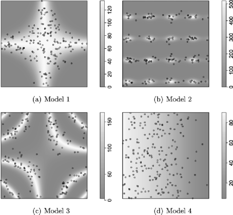
Figure 2: Intensity functions and examples of realizations of Poisson point processes with intensity functions given by models 1–4 (defined in Section 4.1) and generated on the region $[-1,1]^{2}$.

In addition to the Poisson point process, referred to as poisson in the results to follow, two cases of Cox process models are considered, where we are using the terminology and notation introduced in Section 3.3.2:

• An inhomogeneous log-Gaussian Cox process $\mathbf{X}$ where the underlying Gaussian process has an exponential covariance function $c(u,v)=\sigma^{2}\exp(-\|u-v\|/\alpha)$. We refer then to $\mathbf{X}$ as lgcp1 when $\sigma^{2}=0.5$ and $\alpha=1/15$, and as lgcp2 when $\sigma^{2}=1.5$ and $\alpha=1/30$.

• An inhomogeneous Thomas process $\mathbf{X}$ where $\kappa$ is the intensity of the underlying Poisson point process $\mathbf{C}$ and $\sigma$ is the standard deviation of the normal density $f_{\sigma}$, see (20). We refer then to $\mathbf{X}$ as thomas1 when $\kappa=100$ and $\sigma=0.05$, and as thomas2 when $\kappa=300$ and $\sigma=0.1$.

In addition two observation windows are considered: $W=W_{1}=[-1,1]^{2}$ and $W=W_{2}=[-2,2]^{2}$. For each choice of model and observation window, we adjusted the parameter $\beta$ such that the expected number of points, denoted by $\mu^{\star}$, is 200 for the choice $W=W_{1}$ and 800 for the choice $W=W_{2}$ (reflecting the fact that $W_{2}$ is four times larger than $W_{1}$), and then 1000 independent point patterns were simulated using the spatstat package of R Baddeley and Turner [5].

For each of such 1000 replications, we computed the mcle, using the ppm() function of spatstat with a fixed deterministic grid of $80\times 80$ points to discretize the integral in (23). We also computed the vare considering either the test function $h(u)=\operatorname{div}z(u)$ or its modification $h(u)=\operatorname{div}z(u)\eta_{W}(u)$ for various values of $\varepsilon>0$, where the former case can be viewed as a limiting case of the latter one with $\varepsilon=0$. For the other choices of test functions discussed in Section 3.2.2 some preliminary experiments showed that the present choice of test functions led to estimators with the smallest variances.

Among the different models for the intensity function, models 2 and 4 are indeed correctly defined on $\mathbb{R}^{d}$ in the sense that they satisfy at least our condition (ii). To illustrate the simplicity of the vare and the flexibility of conditions (i)–(vi), we focus on model 2 in Appendix B, detail the form of the vare, and show that our asymptotic results are valid.

Figure 3 illustrates some general findings for any choice of point process model and observation window: When the smoothing parameter $\varepsilon$ is at least $5\%$ larger than the side-length of the observation window, the vare is effectively unbiased, and its variance increases as $\varepsilon$ increases. However, when the point process is too much aggregated on the boundary of the observation window (as, e.g., in the case of (b) in Figure 2), a too small value of $\varepsilon$ leads to biased estimates. At the opposite, when the point process is not too much aggregated on the boundary of the observation window (see, e.g., in the case of (a) in Figure 2), the choice $\varepsilon=0$ leads to the smallest variance.

Figure 3: Box plots of mcle and vare for $\theta_{1}$ (the first coordinate of $\theta$) under models 2 and 4, when using the test function $h(u)=\operatorname{div}z(u)\eta_{W}(u)$ for different values of $\varepsilon$, with $\varepsilon=0$ corresponding to $h(u)=\operatorname{div}z(u)$. The plots are based on simulations from Poisson point processes on the observation window $[-2,2]^{2}$, when the expected number of points is 800. Similar results are obtained for the other cases of point process models and choice of observation window.

Table 1: Average of the $p$ empirical mean squared errors (amse) of the estimates for the coordinates in ${\theta}=(\theta_{1},\ldots,\theta_{p})^{\top}$ and based on independent realizations of Poisson, inhomogeneous log-Gaussian Cox processes, and inhomogeneous Thomas point processes with different parameters, intensity functions, and observation windows as described in Section 4.1

	$W_{1}=[-1,1]^{2}$ $(\mu^{\star}=200)$			$W_{2}=[-2,2]^{2}$ $(\mu^{\star}=800)$
	vare			vare
	$\varepsilon=0$	$\varepsilon=0.1$	mcle	$\varepsilon=0$	$\varepsilon=0.2$	mcle
Model 1: ${\theta}=-2$, $z(u)=u_{1}^{2}u_{2}^{2}$
poisson	0.109	0.124	0.085	0.027	0.030	0.022
lgcp1	0.152	0.181	0.143	0.035	0.040	0.032
lgcp2	0.170	0.203	0.143	0.035	0.041	0.033
thomas1	0.141	0.163	0.118	0.033	0.037	0.030
thomas2	0.118	0.147	0.095	0.026	0.027	0.025
Model 2: ${\theta}=(1,4)^{\top}$, $z(u)=(\sin(4\uppi u_{1}),\sin(4\uppi u_{2}))^{\top}$
poisson	0.104	0.126	0.089	0.028	0.033	0.033
lgcp1	0.131	0.159	0.117	0.041	0.047	0.066
lgcp2	0.180	0.213	0.144	0.055	0.062	0.067
thomas1	0.132	0.158	0.106	0.039	0.046	0.062
thomas2	0.106	0.130	0.098	0.035	0.039	0.061
Model 3: ${\theta}=2$, $z(u)=\sin(4\uppi u_{1}u_{2})$
poisson	0.087	0.105	0.037	0.023	0.026	0.010
lgcp1	0.122	0.137	0.052	0.038	0.036	0.023
lgcp2	0.149	0.174	0.057	0.038	0.038	0.023
thomas1	0.103	0.119	0.048	0.033	0.032	0.021
thomas2	0.096	0.109	0.042	0.034	0.031	0.021
Model 4: ${\theta}=(-1,-1,-0.5)^{\top}$, $z(u)=(u_{1},u_{1}^{2},u_{1}^{3})^{\top}$
poisson	0.420	0.410	0.216	1.819	0.027	0.010
lgcp1	0.463	0.556	0.332	1.835	0.035	0.015
lgcp2	0.471	0.588	0.327	1.841	0.035	0.016
thomas1	0.456	0.545	0.277	1.836	0.030	0.012
thomas2	0.427	0.445	0.246	1.805	0.026	0.010

Table 1 concerns the situations with $\varepsilon=0$, $\varepsilon=0.1$ when $W=W_{1}=[-1,1]^{2}$, and $\varepsilon=0.2$ when $W=W_{2}=[-2,2]^{2}$ (in the latter two cases, the choice of $\varepsilon>0$ corresponds to $5\%$ of the side-length of $W$). The table shows the average of the $p$ empirical mean squared errors (abbreviated as amse) of the estimates for the coordinates in ${\theta}=(\theta_{1},\ldots,\theta_{p})^{\top}$ and based on the 1000 replications. In all except a few cases, the amse is smallest for the mcle, the exception being model 2 when $W=W_{2}$. In most cases, the amse is smaller when $\varepsilon=0$ than if $\varepsilon>0$, the exception being some cases of model 3 when $W=W_{2}$ and all cases of model 4 when $W=W_{2}$. For models 1–2, the amse for the vare with $\varepsilon=0$ is rather close to the amse for the mcle. For models 3–4, and in particular model 4 with $W=W_{2}$, the difference is more pronounced, and the amse for the mcle is the smallest.

4.2 Results with a high number of points and varying dimension of space

In this section, we investigate the vare and the mcle when the observed number of points is expected to be very high, when the dimension $d$ varies from 2 to 6, and when the dimension $p$ of $\theta$ scales with $d$. Specifically, we let $p=d$ and consider a Poisson point process with

$$\log\rho(u)=\beta+\sum_{i=1}^{d}\theta_{i}\sin(4\uppi u_{i})/d,\qquad u=(u_{1},\ldots,u_{d})^{\top}\in\mathbb{R}^{d},$$

where $\theta_{1}=\cdots=\theta_{d}=1$, $d=2,\ldots,6$, and $\beta$ is chosen such that the expected number of points in $W=[-1,1]^{d}$ is $\mu^{\star}=10\,000$.

For $d=2,\ldots,6$, we simulated 1000 independent realizations of such a Poisson point process within $W=[-1,1]^{d}$. For each realization, when calculating the mcle we used a systematic grid (i.e., a square, cubic$,\ldots$ grid when $d=2,3,\ldots$) for the discretization of the integral in (23), where the number of dummy points $n_{D}$ is equal to $\tau\mu^{\star}$ with $\tau=0.1,0.5,1,2,4,10$.

Similar to Table 1, Table 2 shows ratios of amse’s for the two types of estimators, vare and mcle, as the dimension $d$ (and number of parameters) varies and as the number of dummy points $n_{D}$ varies from 1000 to 100 000. In terms of the amse, the vare outperforms the mcle for the smaller values of $n_{D}$, and the two estimators are only equally good at the largest value of $n_{D}$ in Table 2.

Table 2: Ratio of the amse of the mcle over the amse of the vare for $\theta=(\theta_{1},\ldots,\theta_{d})\in\mathbb{R}^{d}$ and based on simulations from Poisson point processes as described in Section 4.2. The rows corresponds to the dimension (and number of parameters) $d$, and the columns to the number of dummy points $n_{D}=10\,000\tau$ used to discretize the integral of (23) when calculating the mcle

	$\mbox{{amse}}_{\mathrm{MCLE}}/\mbox{{amse}}_{\mathrm{VARE}}$
	$\tau=0.1$	$\tau=0.5$	$\tau=1$	$\tau=2$	$\tau=4$	$\tau=10$
$d=2$	11.00	2.71	1.83	1.32	1.08	0.95
$d=3$	11.20	2.77	1.88	1.36	1.15	0.99
$d=4$	11.35	2.92	1.97	1.41	1.16	0.99
$d=5$	11.67	3.00	2.00	1.43	1.21	1.03
$d=6$	10.59	2.92	1.92	1.40	1.17	1.02

Table 3: Average time (in seconds) for the computation of the vare and of the mcle as considered in Table 2

		mcle
	vare	$\tau=0.1$	$\tau=0.5$	$\tau=1$	$\tau=2$	$\tau=4$	$\tau=10$
$d=2$	0.004	0.200	0.347	0.546	0.984	1.929	5.744
$d=3$	0.005	0.178	0.298	0.450	0.779	1.483	4.087
$d=4$	0.007	0.231	0.374	0.562	0.941	1.740	4.805
$d=5$	0.009	0.272	0.432	0.650	1.082	1.994	5.493
$d=6$	0.011	0.312	0.494	0.739	1.242	2.367	6.203

Table 3 presents the average time in seconds to get one estimate based on the vare and as a function of $d$, and also the average time in seconds to get one estimate based on the mcle and as a function of both $d$ and $\tau$. The table clearly shows how much faster the calculation of the vare than the mcle is. In particular, when $n_{D}=100\,000$, the average computation time of the mcle is around 1400 ($d=2$) to 560 ($d=6$) times slower than that of the vare.

4.3 Results when $z$ is known only on a finite set of locations

The calculation of the vare based on a realization $\mathbf{X}_{W}=\mathbf{x}$ requires the knowledge of $\operatorname{div}z(u)$ (and possibly also $\operatorname{div}\operatorname{div}z(u)$) for $u\in\mathbf{x}$. In practice, $z$ is often only known for a finite set of points in $W$, which is usually given by a systematic grid imposed on $W$, and we propose then to approximate $\operatorname{div}z$ and $\operatorname{div}\operatorname{div}z$ using the finite-difference method. We discuss below some interesting findings when such an approximation is used.

We focus on the planar case $d=2$, and let $h(u)=\operatorname{div}z(u)$ for the vare. For the two choices of observation windows, $W=W_{1}=[-1,1]^{2}$ or $W=W_{2}=[-2,2]^{2}$, we simulated 1000 realizations of a Poisson point process with $\log\rho(u)=\beta+\sin(4\uppi u_{1})+\sin(4\uppi u_{2})$ for $u=(u_{1},u_{2})\in\mathbb{R}^{2}$ (i.e., model 2 in Section 4.1 with $\theta_{1}=\theta_{2}=1$), where $\beta$ is chosen such that the expected number of points is $\mu^{\star}=200$ if $W=W_{1}$ and $\mu^{\star}=800$ if $W=W_{2}$. For each replication, we calculated four types of estimators, namely vare and mcle which correspond to the situation in Table 1 where $z$ is assumed to be known on $W$, and two “local” versions vare(loc) and mcle(loc) where only knowledge about $z$ on a grid is used. In detail:

• Assuming the full information about $z$ on $W$, vare and mcle were calculated, where for the mcle the integral in (23) is discretized over a quadratic grid $G$ of $n_{D}^{2}$ points in $W$, with $n_{D}=20,40,80$ if $W=W_{1}$, and $n_{D}=40,80,160$ if $W=W_{2}$.

• For each simulated point $u$ of a replication, the $3\times 3$ subgrid whose midpoint is closest to $u$ was used for approximating $\operatorname{div}z(u)$ and $\operatorname{div}\operatorname{div}z(u)$ by the finite-difference method. Thereby, a subgrid $G_{0}\subseteq G$ was obtained as illustrated in Figure 4. Using only the knowledge about $z$ on $G_{0}$, vare(loc) as an approximation of vare was obtained. Furthermore, mcle(loc) was calculated by discretizing the integral in (23) over the grid points in $G_{0}$.

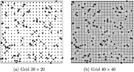
Figure 4: The crosses represent a realization of the Poisson point process under the model 2 and within the observation window $[-1,1]^{2}$. The empty circles represent the grid points where the spatial function $z$ is sampled and used to compute vare(loc) and mcle(loc). The grid points used to compute the mcle correspond to the empty and filled circles.

Table 4: amse for the four types of estimators vare, vare(loc), mcle, and mcle(loc) obtained using different grids as described in Section 4.3. The vare is assuming that the spatial function $z$ is known and is used here as a reference; it does not depend on the refinement of the grid. The results are based on 1000 independent realizations of a planar Poisson point process simulated on the observation window $W=[-1,1]^{2}$ or $W=[-2,2]^{2}$

	$W=[-1,1]^{2}$ $(\mu^{\star}=200)$			$W=[-2,2]^{2}$ $(\mu^{\star}=800)$
	$20\times 20$	$40\times 40$	$80\times 80$	$40\times 40$	$80\times 80$	$160\times 160$
vare	$-$	0.023	$-$	$-$	0.006	$-$
vare(loc)	0.072	0.029	0.025	0.035	0.008	0.006
mcle	0.014	0.014	0.013	0.004	0.004	0.003
mcle(loc)	0.014	0.166	0.628	0.004	0.164	0.623

Table 4 shows that in terms of the amse, the vare(loc) is effectively as good as the vare if the grid is sufficiently fine, cf. the results in the case of the $80\times 80$ grid for $W_{1}$ and the $160\times 160$ grid for $W_{2}$. As expected the mcle performs better than the other estimators, in particular as the grid becomes finer, except for the coarsest grids (the $20\times 20$ grid for $W_{1}$ and the $40\times 40$ grid for $W_{2}$) where the amse is equal for the mcle and the mcle(loc). As the grid gets finer, the amse for the mcle(loc) increases and becomes much larger than for any of the other estimators – only for the coarsest grids, the mcle(loc) and the mcle perform equally good. Thus if the covariates are observed only in a small neighborhood of the location points, it becomes advantageous to use the vare as compared to the mcle. This feature could be of relevance in practice if the covariates are only determined at locations close to the points of $\mathbf{X}_{W}$.

Appendix A Proofs

This Appendix verifies Theorem 3.5 and some accompanying lemmas assuming that $d\geq 2$ and conditions (i)–(vi) in Section 3.3.1 are satisfied.

To simplify the notation, when considering a mean value which possibly depends on $(\beta,{\theta})$, we suppress this and simply write $\mathrm{E}[\cdots]$.

We start by showing that we can replace:

1. the domain $W_{n}$ by a more convenient domain $W_{n}^{\star}$ satisfying $|W_{n}|\sim|W_{n}^{\star}|$ as $n\to\infty$ (meaning that $|W_{n}|/|W_{n}^{\star}|\rightarrow 1$ as $n\to\infty$);

2. the function $h^{(n)}$ by a function $h_{\varepsilon}^{(n)}$ with compact support on $W_{n}^{\star}$, where $\varepsilon=\varepsilon_{n}$ depends on $n$ and should be distinct from the $\varepsilon$ used in (13).

This will later allow us to apply Corollary 3.3.

Let $C_{i}=i+(-1/2,1/2]^{d}$ be the unit box centered at $i\in\mathbb{Z}^{d}$. Define $\mathcal{I}_{n}=\{i\in\mathbb{Z}^{d}\colon\ C_{i}\subset W_{n}\}$, and let $\partial\mathcal{I}_{n}=\{i\in\mathbb{Z}^{d}\setminus\mathcal{I}_{n}\colon\ C_{i}\cap W_{n}\neq\varnothing\}$ be the nearest neighbourhood of $\mathcal{I}_{n}$ on the integer lattice $\mathbb{Z}^{d}$. Set $W_{\partial\mathcal{I}_{n}}=\bigcup_{i\in\partial\mathcal{I}_{n}}C_{i}$ and $W_{n}^{\star}=\bigcup_{i\in\mathcal{I}_{n}}C_{i}$.

Lemma A.1

For any $n=1,2,\ldots\,$, we have $W_{n}^{\star}\subseteq W_{n}\subseteq W_{n}^{\star}\cup W_{\partial\mathcal{I}_{n}}$. As $n\to\infty$, then $|W_{n}|=|A|n^{d}\sim|W_{n}^{\star}|$ and $|W_{n}\setminus W_{n}^{\star}|=\mathcal{O}(n^{d-1})$. Moreover, $\sum_{n\geq 1}|\mathcal{I}_{n}|^{-1}<\infty$.

[Proof.] The first statement is clearly true. Thus, $|W_{n}^{\star}|\leq|W_{n}|\leq|W_{n}^{\star}|+|\partial\mathcal{I}_{n}|$.

By (i), $W_{n}=nA$ is convex, so $|\partial\mathcal{I}_{n}|\leq K_{d}\delta(A)^{d-1}n^{d-1}$, where $\delta(A)$ denotes the diameter of $A$ and $K_{d}>0$ is a constant. Consequently,

$$1\geq\frac{|W_{n}^{\star}|}{|W_{n}|}\geq 1-\frac{|\partial\mathcal{I}_{n}|}{|W_{n}|}\geq 1-\frac{\delta(A)^{d-1}}{n}$$

leading to $|W_{n}|\sim|W_{n}^{\star}|$ as $n\to\infty$. Since $|W_{n}\setminus W_{n}^{\star}|/|W_{n}|\leq K_{d}\delta(A)^{d-1}/n=\mathcal{O}(1/n)$, we obtain $|W_{n}\setminus W_{n}^{\star}|=\mathcal{O}(n^{d-1})$, whereby the second statement is verified.

The last statement follows from that $|\mathcal{I}_{n}|=|W_{n}^{\star}|\sim|A|n^{d}$ and $d\geq 2$.

Now, let $\varepsilon=\varepsilon_{n}=n^{\alpha}$ for some given $\alpha\in[0,1)$. Define $h_{\varepsilon}^{(n)}$ as the regularized function of $h^{(n)}$ as described in Section 3.2 and given by

$$h_{\varepsilon}^{(n)}(u)=h^{(n)}(u)\eta_{W_{n}^{\star}}(u),$$ (24)

where $\eta_{W_{n}^{\star}}$ is defined by (13) (when $W$ is replaced by $W_{n}^{\star}$ and the $\varepsilon$ in (13) is replaced by the present $\varepsilon=\varepsilon_{n}$). By Lemma 3.4 and (i)–(ii), we have that $h_{\varepsilon}^{(n)}$ respective $\operatorname{div}h_{\varepsilon}^{(n)}$ agrees with $h^{(n)}$ respective $\operatorname{div}h^{(n)}$ on ${W_{n}^{\star}}_{\ominus 2\varepsilon}$, the support of $h_{\varepsilon}^{(n)}$ is included in the bounded set $W_{n}^{\star}$, and there exists $K<\infty$ such that

$$\sup_{n\geq 1}\bigl{\|}h_{\varepsilon}^{(n)}\bigr{\|}_{\infty}\leq K\quad\mbox{and}\quad\sup_{n\geq 1}\bigl{\|}\operatorname{div}h_{\varepsilon}^{(n)}-\operatorname{div}h^{(n)}\bigr{\|}_{\infty}\leq K.$$ (25)

The following lemma concerns the behavior of variance functionals computed on $W_{n}$ or $W_{n}^{\star}$.

Lemma A.2

Let $(\psi^{(n)})_{n\geq 1}$ be a sequence of functions in $\mathcal{C}^{0}_{d,1}$ such that

$$\sup_{n\geq 1}\bigl{\|}\psi^{(n)}\bigr{\|}_{\infty}\leq C$$ (26)

for some constant $C<\infty$, then for $\widetilde{W}_{n}=W_{n},W_{n}^{\star}$, the variance

$$V_{\widetilde{W}_{n}}=\operatorname{Var}\biggl{(}\sum_{u\in\mathbf{X}_{\widetilde{W}_{n}}}\psi^{(n)}(u)\biggr{)}$$

is finite and is given by

$$V_{\widetilde{W}_{n}}=\int_{\widetilde{W}_{n}}\psi^{(n)}(u)^{2}\rho(u)\,\mathrm{d}u+\int_{\widetilde{W}_{n}}\int_{\widetilde{W}_{n}}\psi^{(n)}(u)\psi^{(n)}(v)Q_{2}(u,v)\,\mathrm{d}u\,\mathrm{d}v=\mathcal{O}\bigl{(}n^{d}\bigr{)}.$$ (27)

[Proof.] The finiteness of the variance follows from (iv), and the first identity in (27) is immediately derived from (3)–(4).

For the second identity, we consider first $\widetilde{W}_{n}=W_{n}^{\star}$. Define $Y_{i}^{(n)}=\sum_{u\in C_{i}}\psi^{(n)}(u)$ for $i\in\mathcal{I}_{n}$. For $\delta\geq 1$ given in (iv), it is clear that $\mathrm{E}(|Y_{i}^{(n)}|^{2+\delta})$ is bounded by a linear combination of

$$s_{k}^{(n)}=\int_{C_{i}}\cdots\int_{C_{i}}\bigl{|}\psi^{(n)}(u_{1})\cdots\psi^{(n)}(u_{k})\bigr{|}\rho^{(k)}(u_{1},\ldots,u_{k})\,\mathrm{d}u_{1}\cdots\mathrm{d}u_{k},\qquad k=1,\ldots,2+\delta.$$

Using (26) and (iv), we obtain

$$\sup_{n\geq 1}s_{k}^{(n)}\leq C^{k}\sup_{i\in\mathbb{Z}^{d}}\int_{C_{i}}\cdots\int_{C_{i}}\rho^{(k)}(u_{1},\ldots,u_{k})\,\mathrm{d}u_{1}\cdots\mathrm{d}u_{k}\leq C^{k}K^{\prime}<\infty.$$

Therefore,

$$M_{Y}:=\sup_{n\geq 1}\sup_{i\in\mathcal{I}_{n}}\mathrm{E}\bigl{(}\bigl{|}Y_{i}^{(n)}\bigr{|}^{2+\delta}\bigr{)}<\infty.$$

Further, we have the following bound for the covariance in terms of the mixing coefficients of $\mathbf{X}$ (see Doukhan [12] or Guyon [17], remark, page 110),

$$\bigl{|}\operatorname{Cov}\bigl{(}Y_{i}^{(n)},Y_{j}^{(n)}\bigr{)}\bigr{|}\leq 8M_{Y}^{2}\alpha_{1,1}\bigl{(}|j-i|\bigr{)}^{{\delta}/({2+\delta})}.$$

Furthermore, since for any $m\geq 1$, $\alpha_{1,1}(m)\leq\alpha_{2,\infty}(m)$, and since $|W_{n}^{\star}|=|\mathcal{I}_{n}|$, we obtain

$$\bigl{|}W_{n}^{\star}\bigr{|}^{-1}V_{W_{n}^{\star}} = |\mathcal{I}_{n}|^{-1}\sum_{i,j\in\mathcal{I}_{n}}\operatorname{Cov}\bigl{(}Y_{i}^{(n)},Y_{j}^{(n)}\bigr{)}$$

$$\leq 8M_{Y}^{2}|\mathcal{I}_{n}|^{-1}\sum_{i,j\in\mathcal{I}_{n}}\alpha_{2,\infty}\bigl{(}|j-i|\bigr{)}^{\delta/(2+\delta)}$$

$$\leq 8M_{Y}^{2}\sum_{m\geq 0}\bigl{|}\bigl{\{}j\in\mathbb{Z}^{d}\colon\ |j|=m\bigr{\}}\bigr{|}\alpha_{2,\infty}(m)^{\delta/(2+\delta)}$$

$$\leq c_{d}\sum_{m\geq 1}m^{d-1}\alpha_{2,\infty}(m)^{\delta/(2+\delta)},$$

where $c_{d}>0$ is a constant depending only on $d$. Combining this with (v) leads to $|W_{n}^{\star}|^{-1}V_{W_{n}^{\star}}=\mathcal{O}(1)$.

Second, let $\mathcal{J}_{n}=\mathcal{I}_{n}\cup\partial\mathcal{I}_{n}$. Then

$$V_{W_{n}}=\sum_{i,j\in\mathcal{J}_{n}}\operatorname{Cov}\bigl{(}Z_{i}^{(n)},Z_{j}^{(n)}\bigr{)}\qquad\mbox{where for }i\in\mathcal{J}_{n},\qquad Z_{i}^{(n)}=\sum_{u\in X_{C_{i}\cap W_{n}}}\psi^{(n)}(u).$$

Using (26), (iv), and similar arguments as above for the case $\widetilde{W}_{n}=W_{n}$, it is clear that

$$M_{Z}:=\sup_{n\geq 1}\sup_{i\in\mathcal{J}_{n}}\mathrm{E}\bigl{(}\bigl{|}Z_{i}^{(n)}\bigr{|}^{2+\delta}\bigr{)}<\infty.$$

Finally, using (v) and similar arguments as above, we obtain that $|\mathcal{J}_{n}|^{-1}V_{W_{n}}=\mathcal{O}(1)$. This completes the proof, since $|\mathcal{J}_{n}|\sim|\mathcal{I}_{n}|=\mathcal{O}(n^{d})$.

Similar to the definitions of $A_{n}(\mathbf{X})$ and $b_{n}(\mathbf{X})$ in Section 3.2, we define

$$A_{n}^{\star}(\mathbf{X})=\sum_{u\in\mathbf{X}_{W_{n}^{\star}}}h_{\varepsilon}^{(n)}(u)\operatorname{div}z(u)^{\top}\quad\mbox{and}\quad b_{n}^{\star}(\mathbf{X})=\sum_{u\in\mathbf{X}_{W_{n}^{\star}}}\operatorname{div}h_{\varepsilon}^{(n)}(u).$$

We simplify the notation by suppressing the dependence on $\mathbf{X}$ for the random matrices $A_{n}=A_{n}(\mathbf{X})$ and $A_{n}^{\star}=A_{n}^{\star}(\mathbf{X})$, and for the random vectors $b_{n}=b_{n}(\mathbf{X})$ and $b_{n}^{\star}=b_{n}^{\star}(\mathbf{X})$.

Lemma A.3

(I) For $Z_{n}=A_{n},A_{n}^{\star},b_{n},b_{n}^{\star}$, we have $|W_{n}|^{-1}(Z_{n}-\mathrm{E}Z_{n})\stackrel{{\scriptstyle\mathit{a.s.}}}{{\longrightarrow}}0$ as $n\to\infty$.

I(II) $|W_{n}|^{-1}\mathrm{E}(A_{n}{\theta}+b_{n})=\mathcal{O}({n^{\alpha-1}})$.

(III) $(A_{n}-A_{n}^{\star}){\theta}+b_{n}-b_{n}^{\star}=\mathrm{o}_{P}(|W_{n}|^{1/2})=\mathrm{o}_{P}(n^{d/2})$.

[Proof.] (I): We have

$$A_{n}-\mathrm{E}A_{n} = \biggl{(}\sum_{u\in X_{W_{n}}}h^{(n)}(u)\operatorname{div}z(u)^{\top}\biggr{)}-\int_{W_{n}}h^{(n)}(u)\operatorname{div}z(u)^{\top}\rho(u)\,\mathrm{d}u,$$

$$A_{n}^{\star}-\mathrm{E}A_{n}^{\star} = \biggl{(}\sum_{u\in X_{W_{n}^{\star}}}h_{\varepsilon}^{(n)}(u)\operatorname{div}z(u)^{\top}\biggr{)}-\int_{W_{n}^{\star}}h_{\varepsilon}^{(n)}(u)\operatorname{div}z(u)^{\top}\rho(u)\,\mathrm{d}u,$$

$$b_{n}-\mathrm{E}b_{n} = \biggl{(}\sum_{u\in X_{W_{n}}}\operatorname{div}h^{(n)}(u)\biggr{)}-\int_{W_{n}}\operatorname{div}h^{(n)}(u)\rho(u)\,\mathrm{d}u,$$

$$b_{n}^{\star}-\mathrm{E}b_{n}^{\star} = \biggl{(}\sum_{u\in X_{W_{n}^{\star}}}\operatorname{div}h_{\varepsilon}^{(n)}(u)\biggr{)}-\int_{W_{n}^{\star}}\operatorname{div}h_{\varepsilon}^{(n)}(u)\rho(u)\,\mathrm{d}u.$$

Let $j,k\in\{1,\ldots,p\}$. From (ii) and (27), we obtain

$$\mathrm{E}\bigl{(}(A_{n}-\mathrm{E}A_{n})_{jk}^{2}\bigr{)}=\mathcal{O}\bigl{(}n^{d}\bigr{)},\qquad\mathrm{E}\bigl{(}(b_{n}-\mathrm{E}b_{n})_{j}^{2}\bigr{)}=\mathcal{O}\bigl{(}n^{d}\bigr{)},$$

$$\mathrm{E}\bigl{(}\bigl{(}A_{n}^{\star}-\mathrm{E}A_{n}^{\star}\bigr{)}_{jk}^{2}\bigr{)}=\mathcal{O}\bigl{(}n^{d}\bigr{)},\qquad\mathrm{E}\bigl{(}\bigl{(}b_{n}^{\star}-\mathrm{E}b_{n}^{\star}\bigr{)}_{j}^{2}\bigr{)}=\mathcal{O}\bigl{(}n^{d}\bigr{)}.$$

Hence, for $Z_{n}=A_{n},A_{n}^{\star},b_{n},b_{n}^{\star}$, we have (setting $k=1$ for $Z_{n}=b_{n},b_{n}^{\star}$)

$$\operatorname{Var}\bigl{(}|W_{n}|^{-1}({Z_{n}})_{jk}\bigr{)}=\mathcal{O}\bigl{(}n^{-d}\bigr{)},$$

which together with the Borel–Cantelli lemma and the fact that $d\geq 2$ imply the result of (I).

I(II): By Lemma 3.4 and (24)–(25), we have

$$A_{n}-A_{n}^{\star}=\sum_{u\in\mathbf{X}_{W_{n}^{\star}\setminus{W_{n}^{\star}}_{\ominus 2\varepsilon}}}\bigl{(}h^{(n)}(u)-h_{\varepsilon}^{(n)}(u)\bigr{)}\operatorname{div}z(u)^{\top}+\sum_{u\in\mathbf{X}_{W_{n}\setminus{W_{n}^{\star}}}}h^{(n)}(u)\operatorname{div}z(u)^{\top}$$ (28)

and

$$b_{n}-b_{n}^{\star}=\sum_{u\in W_{n}^{\star}\setminus{W_{n}^{\star}}_{\ominus 2\varepsilon}}\bigl{(}\operatorname{div}h^{(n)}(u)-\operatorname{div}h_{\varepsilon}^{(n)}(u)\bigr{)}+\sum_{u\in W_{n}\setminus{W_{n}^{\star}}}\operatorname{div}h^{(n)}(u).$$ (29)

We denote by $T_{1}$ and $T_{2}$ the two sums of the right-hand side of (28) and by $T^{\prime}_{1}$ and $T^{\prime}_{2}$ the two sums of the right-hand side of (29). Using (ii), (3), and (25), we obtain $\mathrm{E}T_{1}=\mathcal{O}(|W_{n}^{\star}\setminus{W_{n}^{\star}}_{\ominus 2\varepsilon}|)$, $\mathrm{E}T_{2}=\mathcal{O}(|W_{n}\setminus{W_{n}^{\star}}|)$, $\mathrm{E}T_{1}^{\prime}=\mathcal{O}(|W_{n}^{\star}\setminus{W_{n}^{\star}}_{\ominus 2\varepsilon}|)$, and $\mathrm{E}T_{2}^{\prime}=\mathcal{O}(|W_{n}\setminus{W_{n}^{\star}}|)$. By Lemma A.1, $|W_{n}\setminus{W_{n}^{\star}}|=\mathcal{O}(n^{d-1})$ and $|W_{n}^{\star}\setminus{W_{n}^{\star}}_{\ominus 2\varepsilon}|=\mathcal{O}(n^{d-1+\alpha})$, since $\alpha<1$. Hence,

$$\mathrm{E}\bigl{(}\bigl{(}A_{n}-A_{n}^{\star}\bigr{)}{\theta}\bigr{)}=\mathcal{O}\bigl{(}n^{d-1+\alpha}\bigr{)}+\mathcal{O}\bigl{(}n^{d-1}\bigr{)}=\mathcal{O}\bigl{(}n^{d-1+\alpha}\bigr{)}$$ (30)

and

$$\mathrm{E}\bigl{(}b_{n}-b_{n}^{\star}\bigr{)}=\mathcal{O}\bigl{(}n^{d-1+\alpha}\bigr{)}+\mathcal{O}\bigl{(}n^{d-1}\bigr{)}=\mathcal{O}\bigl{(}n^{d-1+\alpha}\bigr{)}.$$ (31)

Since $h_{\varepsilon}^{(n)}$ has support included in $W_{n}^{\star}$, Corollary 3.3 gives $\mathrm{E}(A_{n}^{\star}{\theta}+b_{n}^{\star})=0$. Combining this with (30)–(31) gives the result of (II).

(III): From Lemmas A.1–A.2, (ii), and (25), we get

$$\operatorname{Var}T_{1}=\mathcal{O}\bigl{(}\bigl{|}W_{n}^{\star}\setminus{W_{n}^{\star}}_{\ominus 2\varepsilon}\bigr{|}\bigr{)}=\mathcal{O}\bigl{(}n^{d-1+\alpha}\bigr{)}$$

and

$$\operatorname{Var}T_{2}=\mathcal{O}\bigl{(}\bigl{|}W_{n}\setminus{W_{n}^{\star}}\bigr{|}\bigr{)}=\mathcal{O}\bigl{(}n^{d-1}\bigr{)},$$

which leads to

$$\operatorname{Var}\bigl{(}|W_{n}|^{-1/2}\bigl{(}A_{n}-A_{n}^{\star}\bigr{)}{\theta}\bigr{)}=\mathcal{O}\biggl{(}\frac{n^{d-1+\alpha}}{n^{d}}\biggr{)}=\mathcal{O}\bigl{(}{n^{\alpha-1}}\bigr{)}.$$ (32)

In the same way, we derive

$$\operatorname{Var}T_{1}^{\prime}=\mathcal{O}\bigl{(}\bigl{|}W_{n}^{\star}\setminus{W_{n}^{\star}}_{\ominus 2\varepsilon}\bigr{|}\bigr{)}=\mathcal{O}\bigl{(}n^{d-1+\alpha}\bigr{)}$$

and

$$\operatorname{Var}T_{2}^{\prime}=\mathcal{O}\bigl{(}\bigl{|}W_{n}\setminus W_{n}^{\star}\bigr{|}\bigr{)}=\mathcal{O}\bigl{(}n^{d-1}\bigr{)},$$

which leads to

$$\operatorname{Var}\bigl{(}|W_{n}|^{-1/2}\bigl{(}b_{n}-b_{n}^{\star}\bigr{)}\bigr{)}=\mathcal{O}\bigl{(}{n^{\alpha-1}}\bigr{)}.$$ (33)

Combining (32)–(33) with Chebyshev’s inequality completes the proof of (III).

Finally, we turn to the proof of (a)–(c) in Theorem 3.5.

(a): With probability one, by (I) in Lemma A.3, $|W_{n}|^{-1}(A_{n}-S_{n})\geq-|W_{n}|^{-1}S_{n}/2$ for all sufficiently large $n$, and so by (iii),

$$\frac{A_{n}}{|W_{n}|}\geq\frac{S_{n}}{2|W_{n}|}\geq\frac{I_{0}}{2}$$ (34)

for all sufficiently large $n$. Thereby, (a) is obtained.

(b): With probability one, for $n$ large enough, we can write $|W_{n}|^{-1}A_{n}({\widehat{\theta}_{n}}-{\theta})=-|W_{n}|^{-1}\*(A_{n}{\theta}+b_{n})$, and by (34), $\|(|W_{n}|^{-1}A_{n})^{-1}\|\leq 2/\mu_{\min}$ where $\mu_{\min}$ is the smallest eigenvalue of $I_{0}$. Combining this with (a) in Theorem 3.5, with probability one, for $n$ large enough, we obtain

$$\|{\widehat{\theta}_{n}}-{\theta}\| = \bigl{\|}\bigl{(}|W_{n}|^{-1}{A_{n}}\bigr{)}^{-1}|W_{n}|^{-1}(A_{n}{\theta}+b_{n})\bigr{\|}$$

$$\leq \frac{2}{\mu_{\min}}\bigl{\|}|W_{n}|^{-1}(A_{n}{\theta}+b_{n})\bigr{\|}.$$

The right-hand side of this inequality converges almost surely to zero, cf. Lemma A.3. Thereby (b) follows.

(c): For a function $\psi\colon\ \mathbb{R}^{d}\to\mathbb{R}$ and a bounded Borel set $\Delta\subset\mathbb{R}^{d}$, define

$$V_{\Delta}(\psi)=\int_{\Delta}\psi(u)\psi(u)^{\top}\rho(u)\,\mathrm{d}u+\int_{\Delta}\int_{\Delta}\psi(u_{1})\psi(u_{2})^{\top}Q_{2}(u_{1},u_{2})\,\mathrm{d}u_{1}\,\mathrm{d}u_{2}$$ (35)

provided the integrals exist (are finite). Observe that $\Sigma_{n}=V_{W_{n}}(f^{(n)}_{\theta})$ and $\Sigma_{n}^{\star}=V_{W_{n}^{\star}}(f^{(n)}_{{\theta},\varepsilon})$ where

$$f^{(n)}_{{\theta},\varepsilon}(u)=h^{(n)}_{\varepsilon}(u)\operatorname{div}z(u)^{\top}{\theta}+\operatorname{div}h_{\varepsilon}^{(n)}(u).$$

We decompose the proof of (c) into three steps.

Step 1. Assuming $\Sigma_{n}^{\star}\geq I_{0}>0$ for some positive definite matrix $I_{0}$ and for all $n$ large enough, we prove that

$${\Sigma_{n}^{\star}}^{-1/2}\bigl{(}A_{n}^{\star}{\theta}+b_{n}^{\star}\bigr{)}\stackrel{{\scriptstyle d}}{{\longrightarrow}}\mathcal{N}(0,I_{p})\qquad\mbox{as $n\rightarrow\infty$}.$$ (36)

We have

$$A_{n}^{\star}{\theta}+b_{n}^{\star}=\sum_{i\in\mathcal{I}_{n}}Y_{i}^{(n)}\qquad\mbox{with }Y_{i}^{(n)}=\sum_{u\in X_{C_{i}}}f^{(n)}_{{\theta},\varepsilon}(u).$$

For any $n\geq 1$ and any $i\in\mathcal{I}_{n}$, $Y_{i}^{(n)}$ has zero mean, and by (iv),

$$\sup_{n\geq 1}\sup_{i\in\mathcal{I}_{n}}\mathrm{E}\bigl{(}\bigl{\|}Y_{i}^{(n)}\bigr{\|}^{2+\delta}\bigr{)}=\mathcal{O}(1).$$

This combined with (v) and the assumption on $\Sigma_{n}^{\star}$, allows us to invoke Karáczony ([25], Theorem 4), which is a central limit theorem for a triangular array of random fields, which in turn is based on Guyon ([17], Theorem 3.3.1). Thereby (36) is obtained.

Step 2. We prove that

$$|W_{n}|^{-1}\bigl{(}\Sigma_{n}-\Sigma_{n}^{\star}\bigr{)}\to 0\qquad\mbox{as $n\rightarrow\infty$}.$$ (37)

Using the notation (35), we have

$$\Sigma_{n}-\Sigma_{n}^{\star}=V_{{W_{n}^{\star}}_{\ominus 2\varepsilon}}\bigl{(}\zeta^{(n)}\bigr{)}+V_{W_{n}\setminus{W_{n}^{\star}}_{\ominus 2\varepsilon}}\bigl{(}\zeta^{(n)}\bigr{)},$$ (38)

where

$$\zeta^{(n)}(u_{1},u_{2})=f^{(n)}_{\theta}(u_{1})f^{(n)}_{\theta}(u_{2})^{\top}-f_{{\theta},\varepsilon}^{(n)}(u_{1})f_{{\theta},\varepsilon}^{(n)}(u_{2})^{\top},\qquad u_{1},u_{2}\in\mathbb{R}^{d}.$$ (39)

By (ii) and (25), every entry of $\zeta^{(n)}(u_{1},u_{2})$ vanishes if $u_{1},u_{2}\in{W_{n}^{\star}}_{\ominus 2\varepsilon}$, and its numeric value is bounded by a constant if $u_{1},u_{2}\in W_{n}$. Therefore, we can apply similar arguments as used in the proof of Lemma A.2 to conclude that

$$|W_{n}|^{-1}\bigl{|}\bigl{(}\Sigma_{n}-\Sigma_{n}^{\star}\bigr{)}_{jk}\bigr{|}=|W_{n}|^{-1}\bigl{(}V_{W_{n}\setminus{W_{n}^{\star}}_{\ominus 2\varepsilon}}\bigl{(}\zeta^{(n)}\bigr{)}\bigr{)}_{jk}=\mathcal{O}\biggl{(}\frac{|W_{n}^{\star}\setminus{W_{n}^{\star}}_{\ominus 2\varepsilon}|}{|W_{n}|}\biggr{)}=\mathcal{O}\bigl{(}n^{\alpha-1}\bigr{)},$$

which leads to the verification of (37).

Step 3. From (vi) and (37), we see that with probability one, $\Sigma_{n}^{\star}$ is invertible for all sufficiently large $n$, which allows us to write

$$\Sigma_{n}^{-1/2}S_{n}({\widehat{\theta}_{n}}-{\theta}) = -\Sigma_{n}^{-1/2}(A_{n}{\theta}+b_{n})$$

$$= -\Sigma_{n}^{-1/2}\bigl{(}\bigl{(}A_{n}-A_{n}^{\star}\bigr{)}{\theta}+b_{n}-b_{n}^{\star}\bigr{)}$$

$${}+\bigl{(}\Sigma_{n}^{-1/2}-\bigl{(}\Sigma_{n}^{\star}\bigr{)}^{-1/2}\bigr{)}\bigl{(}A_{n}^{\star}{\theta}+b_{n}^{\star}\bigr{)}$$

$${}+\bigl{(}\Sigma_{n}^{\star}\bigr{)}^{-1/2}\bigl{(}A_{n}^{\star}{\theta}+b_{n}^{\star}\bigr{)}.$$

From (36) and Slutsky’s lemma, we obtain that (22) will be true if we manage to prove that the two terms (A) and (A) converge towards zero in probability as $n\to\infty$. Let $U_{1}$ and $U_{2}$ denote these two terms. Let $M_{n}=\Sigma_{n}^{\star}/|W_{n}|$. For $n$ large enough, we have $\|M_{n}^{-1}\|\leq 2/{\lambda_{\min}}$, so $\|M_{n}^{-1/2}\|\leq 2/\sqrt{\lambda_{\min}}$, where $\lambda_{\min}$ is the smallest eigenvalue of $I_{0}^{\prime}$ in (vi), and there exists a constant $C$ such that $\max(\|M_{n}^{1/2}\|,\|M_{n}\|)\leq C$. On the first hand, we note that

$$\|U_{1}\|\leq\frac{2}{\sqrt{\lambda_{\min}}}\bigl{\|}|W_{n}|^{1/2}\bigl{(}\bigl{(}A_{n}-A_{n}^{\star}\bigr{)}{\theta}+b_{n}-b_{n}^{\star}\bigr{)}\bigr{\|},$$

which from (III) in Lemma A.3 leads to $U_{1}\stackrel{{\scriptstyle P}}{{\longrightarrow}}0$ as $n\to\infty$. On the other hand, we have

$$U_{2}=\bigl{(}\Sigma_{n}^{-1/2}\bigl{(}\Sigma_{n}^{\star}\bigr{)}^{1/2}-I_{p}\bigr{)}\bigl{(}\Sigma_{n}^{\star}\bigr{)}^{-1/2}\bigl{(}A_{n}^{\star}{\theta}+b_{n}^{\star}\bigr{)}.$$ (42)

Since $\|(\Sigma_{n}/|W_{n}|)^{-1}\|$ is bounded, we derive from (37) that

$$\biggl{(}\frac{\Sigma_{n}}{|W_{n}|}\biggr{)}^{-1}\biggl{(}\frac{\Sigma_{n}-\Sigma_{n}^{\star}}{|W_{n}|}\biggr{)}=I_{p}-{\Sigma}_{n}^{-1}\Sigma_{n}^{\star}\rightarrow 0,$$

which also leads to ${\Sigma}_{n}^{-1/2}(\Sigma_{n}^{\star})^{1/2}\to I_{p}$. Combining (36) and (42) with Slutsky’s lemma, convergence in probability to zero of $U_{2}$ is deduced. The proof of Theorem 3.5 is thereby completed.

Appendix B The vare for model 2

For specificity and simplicity, consider the setting of Section 4.1 when $h(u)=\operatorname{div}z(u)$ and model 2 is assumed. Then a straightforward calculation leads to the following simple expression for the vare:

$${\widehat{\theta}_{n}}=\pmatrix{\displaystyle\sum\cos^{2}(4\uppi u_{1})&\displaystyle\sum\cos(4\uppi u_{1})\cos(4\uppi u_{2})\vspace*{2pt}\cr\displaystyle\sum\cos(4\uppi u_{1})\cos(4\uppi u_{2})&\displaystyle\sum\cos^{2}(4\uppi u_{2})}^{-1}\pmatrix{\displaystyle\sum\sin(4\uppi u_{1})\vspace*{2pt}\cr\displaystyle\sum\sin(4\uppi u_{1})},$$

where $u=(u_{1},u_{2})\in\mathbb{R}^{2}$ and $\sum=\sum_{u\in\mathbf{X}_{W_{n}}}$. In the sequel, we discuss the conditions (i)–(vi) specified in Section 3.3.1.

Conditions (i), (iv), and (v) are discussed in Section 3.3.2 and are satisfied under the setting of Section 4.1. Condition (ii) is obviously satisfied for model 2. Below we focus on condition (iii) as condition (vi) can be checked using similar ideas.

According to the discussion in Section 3.3.2, we only need to verify that $|W_{n}|^{-1}\widetilde{S}_{n}\geq I_{0}$ where

$$\widetilde{S}_{n}=\int_{W_{n}}\operatorname{div}z(u)\operatorname{div}z(u)^{\top}\,\mathrm{d}u.$$

Let $C_{i}$ denote the unit cube centered at $i\in\mathcal{I}_{n}$ where

$$\mathcal{I}_{n}=\bigl{\{}(j,k)\colon\ j,k\in\{-n/2,\ldots,-1/2,1/2,\ldots,n/2\}\bigr{\}}.$$

Then $W_{n}=[-n,n]^{2}=\bigcup_{i\in\mathcal{I}_{n}}C_{i}$. Let $\eta>0$. There exists a non-negative real-valued continuous function $f$ such that $f(\eta)\to 0$ as $\eta\to 0$, and such that for any $i=(i_{1},i_{2})\in\mathcal{I}_{n}$ and any $u=(u_{1},u_{2})\in b((i_{1},i_{1}-3/8),\eta)$

$$\bigl{|}\cos(4\uppi u_{1})-1\bigr{|}\leq f(\eta)\quad\mbox{and}\quad\bigl{|}\cos(4\uppi u_{2})\bigr{|}\leq f(\eta).$$

Therefore, for any $u\in b((i_{1},i_{1}-3/8),\eta)$ and $y\in\mathbb{R}^{2}\setminus\{0\}$, whenever $\eta$ is sufficiently small,

$$y^{\top}\operatorname{div}z(u)\operatorname{div}z(u)^{\top}y$$

$$\quad=16\uppi^{2}\bigl{(}y_{1}^{2}\cos^{2}(4\uppi u_{1})+2y_{1}y_{2}\cos(4\uppi u_{1})\cos(4\uppi u_{2})+y_{2}^{2}\cos^{2}(4\uppi u_{2})\bigr{)}$$

$$\quad\geq 16\uppi^{2}\bigl{(}y_{1}^{2}\bigl{(}1-f(\eta)\bigr{)}-2|y_{1}y_{2}|f(\eta)^{2}-y_{2}^{2}f(\eta)\bigr{)}\geq 8\uppi^{2}y_{1}^{2}.$$

Thus, for sufficiently small $\eta$,

$$y^{\top}\widetilde{S}_{n}y=\sum_{i\in\mathcal{I}_{n}}\int_{C_{i}}y^{\top}\operatorname{div}z(u)\operatorname{div}z(u)^{\top}y\,\mathrm{d}u\geq 8\uppi^{2}y_{1}^{2}\bigl{(}\uppi\eta^{2}\bigr{)}|\mathcal{I}_{n}|=c|W_{n}|$$

with $c=8\uppi^{3}y_{1}^{2}\eta^{2}>0$. This implies that $|W_{n}|^{-1}\widetilde{S}_{n}\geq cJ_{2}$ where $J_{2}$ is the $2\times 2$ identity matrix.

References

- [1] {barticle}[mr] \bauthor\bsnmAlmeida, \bfnmMurilo P.\binitsM.P. &\bauthor\bsnmGidas, \bfnmBasilis\binitsB. (\byear1993). \btitleA variational method for estimating the parameters of MRF from complete or incomplete data. \bjournalAnn. Appl. Probab. \bvolume3 \bpages103–136.\bidissn=1050-5164, mr=1202518\bptokimsref \endbibitem
- [2] {bincollection}[mr] \bauthor\bsnmBaddeley, \bfnmAdrian\binitsA. (\byear2010). \btitleModeling strategies. In \bbooktitleHandbook of Spatial Statistics (\beditor\bfnmA. E.\binitsA.E. \bsnmGelfand, \beditor\bfnmP. J.\binitsP.J. \bsnmDiggle, \beditor\bfnmP.\binitsP. \bsnmGuttorp &\beditor\bfnmM.\binitsM. \bsnmFuentes, eds.). \bseriesChapman & Hall/CRC Handb. Mod. Stat. Methods \bpages339–369. \blocationBoca Raton, FL: \bpublisherCRC Press. \biddoi=10.1201/9781420072884-c20, mr=2730955 \bptokimsref \endbibitem
- [3] {barticle}[auto:STB—2013/06/05—13:45:01] \bauthor\bsnmBaddeley, \bfnmA.\binitsA. &\bauthor\bsnmDereudre, \bfnmA.\binitsA. (\byear2013). \btitleVariational estimators for the parameters of Gibbs point process models. \bjournalBernoulli \bvolume19 \bpages905–930. \bptokimsref \endbibitem
- [4] {barticle}[mr] \bauthor\bsnmBaddeley, \bfnmAdrian\binitsA. &\bauthor\bsnmTurner, \bfnmRolf\binitsR. (\byear2000). \btitlePractical maximum pseudolikelihood for spatial point patterns (with discussion). \bjournalAust. N. Z. J. Stat. \bvolume42 \bpages283–322. \biddoi=10.1111/1467-842X.00128, issn=1369-1473, mr=1794056 \bptnotecheck related\bptokimsref \endbibitem
- [5] {barticle}[auto:STB—2013/06/05—13:45:01] \bauthor\bsnmBaddeley, \bfnmA.\binitsA. &\bauthor\bsnmTurner, \bfnmR.\binitsR. (\byear2005). \btitleSpatstat: An R package for analyzing spatial point patterns. \bjournalJ. Statist. Softw. \bvolume12 \bpages1–42. \bptokimsref \endbibitem
- [6] {barticle}[auto:STB—2013/06/05—13:45:01] \bauthor\bsnmBerman, \bfnmM.\binitsM. &\bauthor\bsnmTurner, \bfnmR.\binitsR. (\byear1992). \btitleApproximating point process likelihoods with GLIM. \bjournalJ. Appl. Stat. \bvolume41 \bpages31–38. \bptokimsref \endbibitem
- [7] {barticle}[mr] \bauthor\bsnmBesag, \bfnmJulian\binitsJ. (\byear1977). \btitleSome methods of statistical analysis for spatial data. \bjournalBulletin of the International Statistical Institute \bvolume47 \bpages77–92. \bptokimsref \endbibitem
- [8] {barticle}[mr] \bauthor\bsnmBolthausen, \bfnmE.\binitsE. (\byear1982). \btitleOn the central limit theorem for stationary mixing random fields. \bjournalAnn. Probab. \bvolume10 \bpages1047–1050. \bidissn=0091-1798, mr=0672305 \bptokimsref \endbibitem
- [9] {bbook}[mr] \bauthor\bsnmDaley, \bfnmD. J.\binitsD.J. &\bauthor\bsnmVere-Jones, \bfnmD.\binitsD. (\byear2003). \btitleAn Introduction to the Theory of Point Processes. Vol. I: Elementary Theory and Methods, \bedition2nd ed. \bseriesProbability and Its Applications (New York). \blocationNew York: \bpublisherSpringer. \bidmr=1950431 \bptokimsref \endbibitem
- [10] {bbook}[mr] \bauthor\bsnmDiggle, \bfnmPeter J.\binitsP.J. (\byear2003). \btitleStatistical Analysis of Spatial Point Patterns, \bedition2nd ed. \blocationLondon: \bpublisherArnold. \bptokimsref \endbibitem
- [11] {bincollection}[mr] \bauthor\bsnmDiggle, \bfnmPeter J.\binitsP.J. (\byear2010). \btitleNonparametric methods. In \bbooktitleHandbook of Spatial Statistics (\beditor\bfnmA. E.\binitsA.E. \bsnmGelfand, \beditor\bfnmP. J.\binitsP.J. \bsnmDiggle, \beditor\bfnmP.\binitsP. \bsnmGuttorp &\beditor\bfnmM.\binitsM. \bsnmFuentes, eds.). \bseriesChapman & Hall/CRC Handb. Mod. Stat. Methods \bpages299–316. \blocationBoca Raton, FL: \bpublisherCRC Press. \biddoi=10.1201/9781420072884-c18, mr=2730936 \bptokimsref \endbibitem
- [12] {bbook}[mr] \bauthor\bsnmDoukhan, \bfnmPaul\binitsP. (\byear1994). \btitleMixing: Properties and Examples. \bseriesLecture Notes in Statistics \bvolume85. \blocationNew York: \bpublisherSpringer. \biddoi=10.1007/978-1-4612-2642-0, mr=1312160 \bptokimsref \endbibitem
- [13] {barticle}[mr] \bauthor\bsnmGuan, \bfnmYongtao\binitsY. (\byear2006). \btitleA composite likelihood approach in fitting spatial point process models. \bjournalJ. Amer. Statist. Assoc. \bvolume101 \bpages1502–1512. \biddoi=10.1198/016214506000000500, issn=0162-1459, mr=2279475 \bptokimsref \endbibitem
- [14] {bmisc}[auto:STB—2013/06/05—13:45:01] \bauthor\bsnmGuan, \bfnmY.\binitsY., \bauthor\bsnmJalilian, \bfnmA.\binitsA. &\bauthor\bsnmWaagepetersen, \bfnmR.\binitsR. (\byear2011). \bhowpublishedOptimal estimation of the intensity function of a spatial point process. Research Report R-2011-14, Dept. Mathematical Sciences, Aalborg Univ. \bptokimsref \endbibitem
- [15] {barticle}[mr] \bauthor\bsnmGuan, \bfnmYongtao\binitsY. &\bauthor\bsnmLoh, \bfnmJi Meng\binitsJ.M. (\byear2007). \btitleA thinned block bootstrap variance estimation procedure for inhomogeneous spatial point patterns. \bjournalJ. Amer. Statist. Assoc. \bvolume102 \bpages1377–1386. \biddoi=10.1198/016214507000000879, issn=0162-1459, mr=2412555 \bptokimsref \endbibitem
- [16] {barticle}[mr] \bauthor\bsnmGuan, \bfnmYongtao\binitsY. &\bauthor\bsnmShen, \bfnmYe\binitsY. (\byear2010). \btitleA weighted estimating equation approach for inhomogeneous spatial point processes. \bjournalBiometrika \bvolume97 \bpages867–880. \biddoi=10.1093/biomet/asq043, issn=0006-3444, mr=2746157 \bptokimsref \endbibitem
- [17] {bbook}[mr] \bauthor\bsnmGuyon, \bfnmXavier\binitsX. (\byear1995). \btitleRandom Fields on a Network: Modeling, Statistics, and Applications. \bseriesProbability and Its Applications (New York). \blocationNew York: \bpublisherSpringer. \bidmr=1344683 \bptnotecheck year\bptokimsref \endbibitem
- [18] {barticle}[mr] \bauthor\bsnmHeinrich, \bfnmL.\binitsL. (\byear1992). \btitleOn existence and mixing properties of germ-grain models. \bjournalStatistics \bvolume23 \bpages271–286. \biddoi=10.1080/02331889208802375, issn=0233-1888, mr=1237805 \bptokimsref \endbibitem
- [19] {bbook}[auto:STB—2013/06/05—13:45:01] \bauthor\bsnmHörmander, \bfnmL.\binitsL. (\byear2003). \btitleThe Analysis of Linear Partial Differential Operators. I. Distribution Theory and Fourier Analysis. \blocationBerlin: \bpublisherSpringer. \bnoteReprint of the second (1990) edition. \bptokimsref \endbibitem
- [20] {bbook}[mr] \bauthor\bsnmIbragimov, \bfnmI. A.\binitsI.A. &\bauthor\bsnmLinnik, \bfnmYu. V.\binitsY.V. (\byear1971). \btitleIndependent and Stationary Sequences of Random Variables. \blocationGroningen: \bpublisherWolters-Noordhoff. \bidmr=0322926 \bptokimsref \endbibitem
- [21] {bbook}[mr] \bauthor\bsnmIllian, \bfnmJanine\binitsJ., \bauthor\bsnmPenttinen, \bfnmAntti\binitsA., \bauthor\bsnmStoyan, \bfnmHelga\binitsH. &\bauthor\bsnmStoyan, \bfnmDietrich\binitsD. (\byear2008). \btitleStatistical Analysis and Modelling of Spatial Point Patterns. \bseriesStatistics in Practice. \blocationChichester: \bpublisherWiley. \bidmr=2384630 \bptokimsref \endbibitem
- [22] {barticle}[mr] \bauthor\bsnmJensen, \bfnmJ. L.\binitsJ.L. (\byear1993). \btitleAsymptotic normality of estimates in spatial point processes. \bjournalScand. J. Stat. \bvolume20 \bpages97–109. \bidissn=0303-6898, mr=1229287 \bptokimsref \endbibitem
- [23] {barticle}[mr] \bauthor\bsnmJensen, \bfnmJens Ledet\binitsJ.L. &\bauthor\bsnmKünsch, \bfnmHans R.\binitsH.R. (\byear1994). \btitleOn asymptotic normality of pseudo likelihood estimates for pairwise interaction processes. \bjournalAnn. Inst. Statist. Math. \bvolume46 \bpages475–486. \bidissn=0020-3157, mr=1309718 \bptokimsref \endbibitem
- [24] {barticle}[mr] \bauthor\bsnmJensen, \bfnmJens Ledet\binitsJ.L. &\bauthor\bsnmMøller, \bfnmJesper\binitsJ. (\byear1991). \btitlePseudolikelihood for exponential family models of spatial point processes. \bjournalAnn. Appl. Probab. \bvolume1 \bpages445–461. \bidissn=1050-5164, mr=1111528 \bptokimsref \endbibitem
- [25] {barticle}[mr] \bauthor\bsnmKarácsony, \bfnmZsolt\binitsZ. (\byear2006). \btitleA central limit theorem for mixing random fields. \bjournalMiskolc Math. Notes \bvolume7 \bpages147–160. \bidissn=1787-2405, mr=2310274 \bptokimsref \endbibitem
- [26] {barticle}[mr] \bauthor\bsnmMøller, \bfnmJesper\binitsJ., \bauthor\bsnmSyversveen, \bfnmAnne Randi\binitsA.R. &\bauthor\bsnmWaagepetersen, \bfnmRasmus Plenge\binitsR.P. (\byear1998). \btitleLog Gaussian Cox processes. \bjournalScand. J. Stat. \bvolume25 \bpages451–482. \biddoi=10.1111/1467-9469.00115, issn=0303-6898, mr=1650019 \bptokimsref \endbibitem
- [27] {bbook}[mr] \bauthor\bsnmMøller, \bfnmJesper\binitsJ. &\bauthor\bsnmWaagepetersen, \bfnmRasmus Plenge\binitsR.P. (\byear2004). \btitleStatistical Inference and Simulation for Spatial Point Processes. \bseriesMonographs on Statistics and Applied Probability \bvolume100. \blocationBoca Raton, FL: \bpublisherChapman & Hall/CRC. \bidmr=2004226 \bptokimsref \endbibitem
- [28] {barticle}[mr] \bauthor\bsnmMøller, \bfnmJesper\binitsJ. &\bauthor\bsnmWaagepetersen, \bfnmRasmus P.\binitsR.P. (\byear2007). \btitleModern statistics for spatial point processes. \bjournalScand. J. Stat. \bvolume34 \bpages643–684. \biddoi=10.1111/j.1467-9469.2007.00569.x, issn=0303-6898, mr=2392447 \bptokimsref \endbibitem
- [29] {barticle}[mr] \bauthor\bsnmPolitis, \bfnmDimitris N.\binitsD.N., \bauthor\bsnmPaparoditis, \bfnmEfstathios\binitsE. &\bauthor\bsnmRomano, \bfnmJoseph P.\binitsJ.P. (\byear1998). \btitleLarge sample inference for irregularly spaced dependent observations based on subsampling. \bjournalSankhyā Ser. A \bvolume60 \bpages274–292. \bidissn=0581-572X, mr=1711685 \bptokimsref \endbibitem
- [30] {barticle}[mr] \bauthor\bsnmProkešová, \bfnmMichaela\binitsM. &\bauthor\bsnmJensen, \bfnmEva B. Vedel\binitsE.B.V. (\byear2013). \btitleAsymptotic Palm likelihood theory for stationary point processes. \bjournalAnn. Inst. Statist. Math. \bvolume65 \bpages387–412. \biddoi=10.1007/s10463-012-0376-7, issn=0020-3157, mr=3011627 \bptnotecheck year\bptokimsref \endbibitem
- [31] {barticle}[mr] \bauthor\bsnmSchoenberg, \bfnmFrederic Paik\binitsF.P. (\byear2005). \btitleConsistent parametric estimation of the intensity of a spatial-temporal point process. \bjournalJ. Statist. Plann. Inference \bvolume128 \bpages79–93. \biddoi=10.1016/j.jspi.2003.09.027, issn=0378-3758, mr=2110179 \bptokimsref \endbibitem
- [32] {bbook}[mr] \bauthor\bsnmStoyan, \bfnmD.\binitsD., \bauthor\bsnmKendall, \bfnmW. S.\binitsW.S. &\bauthor\bsnmMecke, \bfnmJ.\binitsJ. (\byear1995). \btitleStochastic Geometry and Its Applications, \bedition2nd ed. \blocationChichester: \bpublisherWiley. \bptokimsref \endbibitem
- [33] {barticle}[mr] \bauthor\bsnmWaagepetersen, \bfnmRasmus\binitsR. &\bauthor\bsnmGuan, \bfnmYongtao\binitsY. (\byear2009). \btitleTwo-step estimation for inhomogeneous spatial point processes. \bjournalJ. R. Stat. Soc. Ser. B Stat. Methodol. \bvolume71 \bpages685–702. \biddoi=10.1111/j.1467-9868.2008.00702.x, issn=1369-7412, mr=2749914 \bptokimsref \endbibitem
- [34] {barticle}[mr] \bauthor\bsnmWaagepetersen, \bfnmRasmus Plenge\binitsR.P. (\byear2007). \btitleAn estimating function approach to inference for inhomogeneous Neyman–Scott processes. \bjournalBiometrics \bvolume63 \bpages252–258, 315. \biddoi=10.1111/j.1541-0420.2006.00667.x, issn=0006-341X, mr=2345595 \bptokimsref \endbibitem