Transport properties of Lévy walks: an analysis in terms of multistate processes

Abstract

Continuous time random walks combining diffusive and ballistic regimes are introduced to describe a class of Lévy walks on lattices. By including exponentially-distributed waiting times separating the successive jump events of a walker, we are led to a description of such Lévy walks in terms of multistate processes whose time-evolution is shown to obey a set of coupled delay differential equations. Using simple arguments, we obtain asymptotic solutions to these equations and rederive the scaling laws for the mean squared displacement of such processes. Our calculation includes the computation of all relevant transport coefficients in terms of the parameters of the models.

Random walks described by Lévy flights give rise to complex diffusive processes [1, 2, 3, 4] and have found many applications in physics and beyond [5, 6, 7, 8]. Whereas the random walks associated with Brownian motion are characterized by Gaussian propagators whose variance grows linearly in time, the propagators of Lévy flights have infinite variance [9, 10, 11]; they occur in models of random walks such that the probability of a long jump decays slowly with its length [12].

By considering the propagation time between the two ends of a jump, one obtains a class of models known as Lévy walks [13, 14, 15, 16, 17, 18, 19]. A Lévy walker thus follows a continuous path between the two end points of every jump, performing each in a finite time; instead of having an infinite mean squared displacement, as happens in a Lévy flight whose jumps take place instantaneously, a Lévy walker moves with finite velocity and, ipso facto, has a finite mean squared displacement, although it may increase faster than linearly in time.

A Lévy flight is characterized by its probability density of jump lengths $x$, or free paths, which we denote $\phi(x)$. It is assumed to have the asymptotic scaling, $\phi(x)\sim x^{-\alpha-1}$, whose exponent, $\alpha>0$, determines whether the moments of the displacement are finite. In particular, for $\alpha\leq 2$, the variance diverges.

In the framework of continuous time random walks [5, Chs. 10 & 13], a probability distribution $\Phi(\vect{r},t)$ of making a displacement $\vect{r}$ in a time $t$ is introduced, such that, for instance, in the so-called velocity picture, $\Phi(\vect{r},t)=\phi(|\vect{r}|)\delta_{\mathrm{D}}(t-|\vect{r}|/v)$, where $v$ denotes the constant speed of the particle and $\delta_{\mathrm{D}}(.)$ is the Dirac delta function. Considering the Fourier-Laplace transform of the propagator of this process, one obtains, in terms of the parameter $\alpha$, the following scaling laws for the mean squared displacement after time $t$ [13, 20],

$$\langle r^{2}\rangle_{t}\sim\begin{cases}t^{2}\,,&0<\alpha<1\,,\\ t^{2}/\log t\,,&\alpha=1\,,\\ t^{3-\alpha}\,,&1<\alpha<2\,,\\ t\log t\,,&\alpha=2\,,\\ t\,,&\alpha>2\,.\end{cases}$$ (1)

In this Letter, we consider Lévy walks on lattices and generalize the above description, according to which a new jump event takes place as soon as the previous one is completed, to include an exponentially-distributed waiting time which separates successive jumps. This induces a distinction between the states of particles which are in the process of completing a jump and those that are waiting to start a new one. As shown below, such considerations lead to a theoretical formulation of the model as a multistate generalized master equation [21, 22, 23], which translates into a set of coupled delay differential equations for the corresponding distributions.

The physical motivation for the inclusion of an exponentially-distributed waiting time between successive jump events stems, for instance, in the framework of chaotic scattering, from the time required to escape a fractal repeller [24, 25], or, more generally, the time spent in a chaotic transient [26]. In the framework of active transport, such as dealing with the motion of particles embedded within living cells [27], such waiting times may help model the complex process related to changes in the direction of propagation of such particles. This is also relevant to laser cooling experiments [28], where a competition in the damping and increase of atomic momenta induces a form of random walk in momentum space. The times spent by atoms in small momenta states typically follow exponential distributions.

The stop-and-go patterns of random walkers thus generated have been studied in the context of animal foraging [29]. Such search strategies have been termed saltatory. In contrast to classical strategies, according to which animals either move while foraging or stop to ambush their prey, a saltatory searcher alternates between scanning phases, which are performed diffusively on a local scale, and relocation phases, during which motion takes place without search. Examples of such intermittent behaviour have been identified in a variety of animal species [30, 31], as well as in intracellular processes such as proteins binding to DNA strands [32]. Visual searching patterns whereby information is extracted through a cycle of brief fixations interspersed with gaze shifts[33] provide another illustration in the context of neuroscience. One can also think of applications to sociological processes, for instance when interactions between individuals is sampled at random times, independent of the underlying process [34].

From a mathematical perspective, an important question that arises in the framework of foraging is that of optimal strategies [35]. As reported in [36], Lévy flight motion can, under some conditions on the nature and distribution of targets, emerge as an optimal strategy for non-destructive search, i.e., when targets can be visited infinitely often. For destructive searches on the other hand, intermittent search strategies with exponentially-distributed waiting times provide an alternative to Lévy search strategies, which turns out to minimize the search time [37]. The processes we analyze in this Letter, although they are restricted to motion on lattices, can be thought of as extensions of intermittent search processes to power-law distributed relocation phases which are typical of Lévy search strategies, thus opening a new perspective.

We show below that, inasmuch as the dispersive properties are concerned, a complete characterisation of the process can be obtained, which reproduces the scaling laws (1), as well as yields the corresponding transport coefficients, whether normal or anomalous. These results also elucidate the incidence of exponential waiting times on these coefficients.

1 Lévy walks as multistate processes

We call propagating the state of a particle which is in the process of completing a jump. In contrast, the state of a particle waiting to start a new jump is called scattering . Whereas particles switch from propagating to scattering states as they complete a jump, particles in a scattering state can make transitions to both scattering and propagating states; as soon as their waiting time has elapsed, they move on to a neighbouring site and, doing so, may switch to a propagating state and carry their motion on to the next site, or start anew in a scattering state.

We consider a $d$-dimensional cubic lattice of individual cells $\vect{n}\in\mathbb{Z}^{d}$. The state of a walker at position $\vect{n}$ and time $t$ can take on a countable number of different values, specified by two integers, $k\geq 0$ and $j\in\{1,\dots,z\}$, where $z\equiv 2d$ is the coordination number of the lattice. Scattering states are labeled by the state $k=0$ and propagating states by the pair $(k,j)$, such that $k\geq 1$ counts the remaining number of lattice sites the particle has to travel in direction $j$ to complete its jump.

Time-evolution proceeds as follows. After a random waiting time $t$, exponentially-distributed with mean $\tau_{\mathrm{R}}$, a particle in the scattering state $k=0$ changes its state to $(k,j)$ with probability $\rho_{k}/z$, moving its location from site $\vect{n}$ to site $\vect{n}+\vect{e}_{j}$. Conversely, particles which are at site $\vect{n}$ in a propagating state $(k,j)$, $k\geq 1$, jump to site $\vect{n}+\vect{e}_{j}$, in time $\tau_{\mathrm{B}}$, changing their state to $(k-1,j)$.

The waiting time density of the process is the function

$$\psi_{k}(t)=\begin{cases}\tau_{\mathrm{R}}^{-1}e^{-t/\tau_{\mathrm{R}}}\,,&k=0\,,\\ \delta_{\mathrm{D}}(t-\tau_{\mathrm{B}})\,,&k\neq 0\,.\end{cases}$$ (2)

When a step takes place, the transition probability to go from state $(k,j)$ to state $(k^{\prime},j^{\prime})$ is

$$\mathsf{p}_{(k,j),(k^{\prime},j^{\prime})}=\begin{cases}\rho_{k^{\prime}}/z\,,&k=0\,,\\ \delta_{k-1,k^{\prime}}\delta_{j,j^{\prime}}\,,&k\neq 0\,,\end{cases}$$ (3)

where $\delta_{.,.}$ is the Kronecker symbol.

For definiteness, we consider below the following simple parameterisation of the transition probabilities,

$$\rho_{k}=\begin{cases}1-\epsilon\,,&k=0\,,\\ \epsilon\left[k^{-\alpha}-(k+1)^{-\alpha}\right]\,,&k\geq 1\,,\end{cases}$$ (4)

in terms of the parameters $0<\epsilon<1$, which weights scattering states relative to propagating ones, and $\alpha>0$, the asymptotic scaling parameter of free path lengths.

2 Master equation

The probability distribution of particles at site $\vect{n}$ and time $t$, $P(\vect{n},t)$, is a sum of the distributions over the scattering states, $P_{0}(\vect{n},t)$, and propagating states, $P_{k,j}(\vect{n},t)$, $k\geq 1$ and $1\leq j\leq z$. According to eqs. (2) and (3), changes in the distribution of $(k,j)$-states, $k\geq 1$, in cell $\vect{n}$ arise from particles located at cell $\vect{n}-\vect{e}_{j}$ which make a transition from either state $0$ or state $(k+1,j)$. Since the latter transitions can be traced back to changes in the distribution of $(k+1,j)$-states in cell $\vect{n}-\vect{e}_{j}$ at time $\tau_{\mathrm{B}}$ earlier, we can write

$$\partial_{t}P_{k,j}(\vect{n},t) -\partial_{t}P_{k+1,j}(\vect{n}-\vect{e}_{j},t-\tau_{\mathrm{B}})$$ (5)

$$= \frac{\rho_{k}}{z\tau_{\mathrm{R}}}[P_{0}(\vect{n}-\vect{e}_{j},t)-P_{0}(\vect{n}-\vect{e}_{j},t-\tau_{\mathrm{B}})],$$ (6)

which accounts for the fact that a positive $0$-state contribution at time $t$ becomes a negative one at time $t+\tau_{\mathrm{B}}$. Applying this relation recursively, we have

$$\partial_{t}P_{k,j}(\vect{n},t)=\frac{1}{z\tau_{\mathrm{R}}}\sum_{k^{\prime}=1}^{\infty}\rho_{k+k^{\prime}-1}\Big{[}P_{0}(\vect{n}-k^{\prime}\vect{e}_{j},t-(k^{\prime}-1)\tau_{\mathrm{B}})-P_{0}(\vect{n}-k^{\prime}\vect{e}_{j},t-k^{\prime}\tau_{\mathrm{B}})\Big{]}\,.$$ (7)

See eq. (7) next page. Terms lost by $(1,j)$-states in cells $\vect{n}-\vect{e}_{j}$, $j=1,\dots,z$, are gained by the $0$-state in cell $\vect{n}$, which also gains contributions from $0$-state transitions. Since the scattering state also loses particles at exponential rate $1/\tau_{\mathrm{R}}$, we have

$$\!\!\!\partial_{t}P_{0}(\vect{n},t) =\frac{1}{z\tau_{\mathrm{R}}}\sum_{j=1}^{z}\sum_{k=0}^{\infty}\rho_{k}P_{0}(\vect{n}-(k+1)\vect{e}_{j},t-k\tau_{\mathrm{B}})$$ (7)

$$\quad-\frac{1}{\tau_{\mathrm{R}}}P_{0}(\vect{n},t)\,.$$ (8)

It is straightforward to check that eqs. (7) and (8) are consistent with conservation of probability, $\sum_{\vect{n}}P(\vect{n},t)=1$.

3 Fraction of scattering particles

As discussed below, an important role is played by the overall fraction of particles in the scattering state, $S_{0}(t)\equiv\sum_{\vect{n}\in\mathbb{Z}^{d}}P_{0}(\vect{n},t)$. From eq. (8), this quantity is found to obey the following linear delay differential equation,

$$\tau_{\mathrm{R}}\dot{S}_{0}(t)=\sum_{k=1}^{\infty}\rho_{k}S_{0}(t-k\tau_{\mathrm{B}})-\epsilon S_{0}(t)\,.$$ (9)

Given initial conditions, e.g. $S_{0}(t)=0$, $t<0$, and $S_{0}(0)=1$ (all particles start in a scattering state), this equation can be solved by the method of steps [38]. Because the sum of the coefficients on the right-hand side of eq. (9) is zero, the solutions are asymptotically constant and can be classified in terms of the parameter $\alpha$.

For $$\alpha>1 0 \sum_{k=0}^{\infty}\rho_{k}(\tau_{\mathrm{R}}+k\tau_{\mathrm{B}}) \sum_{k=0}^{\infty}k\rho_{k}=\epsilon\zeta(\alpha)$$, the average return time to the -state, , is finite and given in terms of the Riemann zeta function, since . The process is thus positive-recurrent and we have

$$\lim_{t\to\infty}S_{0}(t)=\frac{\tau_{\mathrm{R}}}{\tau_{\mathrm{R}}+\epsilon\tau_{\mathrm{B}}\zeta(\alpha)}\qquad(\alpha>1)\,.$$ (10a)

In the remaining range of parameter values, $$0<\alpha\leq 1 0 \lim_{t\to\infty}S_{0}(t)=0 \alpha\neq 1$$, the process is null-recurrent: the average return time to the -state diverges and . If , the decay is algebraic,

$$\lim_{t\to\infty}(t/\tau_{\mathrm{B}})^{1-\alpha}S_{0}(t)=\frac{\sin(\pi\alpha)}{\pi\epsilon}\frac{\tau_{\mathrm{R}}}{\tau_{\mathrm{B}}}\qquad(0<\alpha<1)\,,$$ (10b)

which can be obtained from a result due to Dynkin [39]; see also Refs. [40, Vol. 2, § XIV.3] and [28, § 4.4]. The case $$\alpha=1$$ is a singular limit with logarithmic decay,

$$\lim_{t\to\infty}\log(t/\tau_{\mathrm{B}})S_{0}(t)=\frac{1}{\epsilon}\frac{\tau_{\mathrm{R}}}{\tau_{\mathrm{B}}}\qquad(\alpha=1)\,.$$ (10c)

4 Mean squared displacement

Assuming an initial position at the origin, the second moment of the displacement is $\langle n^{2}\rangle_{t}=\sum_{\vect{n}\in\mathbb{Z}^{d}}n^{2}P(\vect{n},t)$. Its time-evolution is obtained by differentiating this expression with respect to time and substituting eqs. (7) and (8),

$$\tau_{\mathrm{R}}\frac{\mathrm{d}}{\mathrm{d}t}\langle n^{2}\rangle_{t} =S_{0}(t)+\epsilon\sum_{k=1}^{\infty}\frac{2k+1}{k^{\alpha}}S_{0}(t-k\tau_{\mathrm{B}})\,,$$ (11)

where, using eq. (4), we made use of the identity $\sum_{j=k}^{\infty}\rho_{j}=1$ for $k=0$ and $\epsilon k^{-\alpha}$ otherwise. The time-evolution of the second moment is thus obtained by integrating the fraction of $0$-state particles,

$$\tau_{\mathrm{R}}\langle n^{2}\rangle_{t}=\int_{0}^{t}\!\mathrm{d}s\,S_{0}(s)+\epsilon\sum_{k=1}^{{\lfloor t/\tau_{\mathrm{B}}\rfloor}}\frac{2k+1}{k^{\alpha}}\int_{0}^{t-k\tau_{\mathrm{B}}}\!\mathrm{d}s\,S_{0}(s)\,,$$ (12)

where, assuming the process starts at $t=0$, we set $S_{0}(t)=0$ for $t<0$.

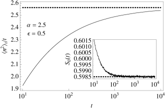
(a)  Normal diffusion, $\alpha=5/2$

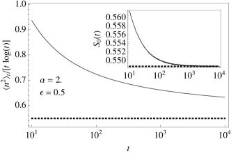
(b)  Weak super-diffusion, $\alpha=2$

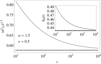
(c)  Super diffusion, $\alpha=3/2$

Figure 1: Examples of numerical computations of $\langle n^{2}\rangle_{t}$ for parameters values $\alpha>1$, rescaled by their respective asymptotic scalings with respect to time ($\epsilon=1/2$ in all cases). The dotted lines correspond to eq. (13b). The insets show the evolution of the fraction of scattering states towards their asymptotic values, given by eq. (10a).

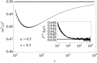
(a)  Ballistic diffusion, $\alpha=1/2$

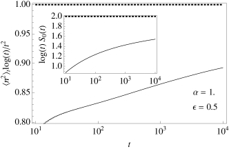
(b)  Sub-ballistic diffusion, $\alpha=1$

Figure 2: Same as fig. 1 for the range of parameters $0<\alpha\leq 1$, with comparisons to eq. (13c) and, in the insets, eqs. (10b) and (10c).

As emphasized earlier, equation (9) can be solved analytically given initial conditions on the state of walkers. By extension, so can equation (12), thus providing an exact time-dependent expression of the mean squared displacement. This is particularly useful when one wishes to study transient regimes and the possibility of a crossover between different scaling behaviours, or indeed when the asymptotic regime remains experimentally or numerically unaccessible. The analytic expression of the mean squared displacement and the issue of the transients will be studied elsewhere. Here, we focus on the asymptotic regime, i.e., $t\gg\tau_{\mathrm{B}}$.

Substituting the asymptotic expressions (10), into eq. (12), we retrieve the regimes described by eq. (1) and obtain the corresponding coefficients.

Starting with the positive-recurrent regime, $$\alpha>1 t\gg\tau_{\mathrm{B}}$$, eq. (10a), we have the three asymptotic regimes, ,

$$\langle n^{2}\rangle_{t} \simeq\frac{t}{\tau_{\mathrm{R}}+\epsilon\tau_{\mathrm{B}}\zeta(\alpha)}$$ (13a)

$$\quad\times\begin{cases}1+\epsilon[\zeta(\alpha)+2\zeta(\alpha-1)]\,,&\alpha>2\,,\\ 2\epsilon\log(t/\tau_{\mathrm{B}})\,,&\alpha=2\,,\\ \frac{2\epsilon}{(2-\alpha)(3-\alpha)}(t/\tau_{\mathrm{B}})^{2-\alpha}\,,&1<\alpha<2\,.\end{cases}$$ (13b)

Whereas the first regime, $$\alpha>2 \alpha=2 1<\alpha<2 3-\alpha>1$$, yields normal diffusion, the other two correspond, for , to a weak form of super-diffusion, and, for , to super-diffusion, such that the mean squared displacement grows with a power of time , faster than linear.

Ballistic diffusion occurs in the null-recurrent regime of the parameter, $0<\alpha\leq 1$. Using eqs. (10b) and (10c), we find

$$\langle n^{2}\rangle_{t}\simeq\frac{t^{2}}{\tau_{\mathrm{B}}^{2}}\begin{cases}1/\log(t/\tau_{\mathrm{B}})\,,&\alpha=1\,,\\ 1-\alpha\,,&0<\alpha<1\,.\end{cases}$$ (13c)

The asymptotic regimes described by eqs. (12) generalize to continuous-time processes similar results found in the context of countable Markov chains applied to discrete time processes [41]. They can also be compared to results obtained in Ref. [42]. Although the Lévy walks considered by these authors do not include exponentially-distributed waiting times separating successive propagating phases, our results are rather similar to theirs; the only actual differences arise in the regime of normal diffusion, $\alpha>2$.

In figs. 1 and 2, the asymptotic results (13) are compared to numerical measurements of the mean squared displacement of the process defined by eqs. (2), (3) and the transition probabilities (4). Timescales were set to $\tau_{\mathrm{R}}\equiv\tau_{\mathrm{B}}\equiv 1$ and the lattice dimension to $d=1$. The algorithm is based on a classic kinetic Monte Carlo algorithm [43], which incorporates the possibility of a ballistic propagation of particles after they undergo a transition from a scattering to a propagating state. For each realisation, the initial state is taken to be scattering. Positions are measured at regular intervals on a logarithmic time scale for times up to $t=10^{4}\tau_{\mathrm{R}}$. Averages are performed over sets of $10^{8}$ trajectories.

5 Concluding remarks

The specificity of our approach to Lévy walks lies in the inclusion of exponentially-distributed waiting times that separate successive jumps. This additional feature induces a natural description of the process in terms of multiple propagating and scattering states whose distributions evolve according to a set of coupled delay differential equations.

The mean squared displacement of the process depends on the distribution of free paths and boils down to a simple expression involving time-integrals of the fraction of scattering states. Using straightforward arguments, precise asymptotic expressions were obtained for this quantity, which reproduce the expected scaling regimes [13, 20], and provide values of the diffusion coefficients, whether normal or anomalous.

Our results confirm that, in the null-recurrent regime of ballistic transport, scattering events, are unimportant. Furthermore, these events do not modify the exponent of the mean squared displacement in the positive recurrent regime; in other words, the addition of a scattering phase has no incidence on the scaling exponents. In this regime, however, the transport coefficients, whether normal or anomalous, depend on the details of the model, underlying the relevance of pausing times that separate long flight events, for example, in the context of animal foraging [36].

Although the results we reported are limited to walks with exponentially distributed waiting times, our formalism can be easily extended to include the possibility of waiting times with power law distributions such as observed in Ref. [44]. Such processes are known to allow for sub-diffusive transport regimes [11]. The combination of two power law scaling parameters, one for the waiting time and the other for the duration of flights, indeed yields a richer set of scaling regimes [45], which can be studied within our framework.

Our results can on the other hand be readily applied to the regime $\tau_{\mathrm{R}}/\tau_{\mathrm{B}}\ll 1$, i.e., such that the waiting times in the scattering state are typically negligible compared to the ballistic timescale. This is the regime commonly studied in reference to Lévy walks.

Our investigation simultaneously opens up new avenues for future work. Among results to be discussed elsewhere, our formalism can be used to obtain exact solutions of the mean squared displacement as a function of time. As discussed already, this is particularly useful to study transient regimes, such as can be observed when the distribution of free paths has a cut-off or, more generally, when it crosses over from one regime to another, e.g. from a power law for small lengths to exponential decay for large ones, or when the anomalous regime is masked by normal sub-leading contributions which may nonetheless dominate over time scales accessible to numerical computations [46]. One can also apply these ideas to the anomalous photon statistics of blinking quantum dots [47, 48]. The on/off switchings of a quantum dot typically exhibit power law distributions. In the limit of strong fields, however, the on-times display exponential cutoffs.

Another interesting regime occurs when, in the positive-recurrent range of the scaling parameter, $\alpha>1$, the likelihood of a transition from a scattering to a propagating state is small, $\epsilon\ll 1$. A similar perturbative regime arises in the infinite horizon Lorentz gas in the limit of narrow corridors [49]. As is well-known [50], the scaling parameter of the distribution of free paths has the marginal value $\alpha=2$, such that the mean squared displacement asymptotically grows with $t\log t$. Although it has long been acknowledged that the infinite horizon Lorentz gas exhibits features similar to a Lévy walk [51, 52], we argue that a consistent treatment of this model in such terms is not possible unless exponentially-distributed waiting times are taken into account that separate successive jumps. Indeed, the parameter $\epsilon$, which weights the likelihood of a transition from scattering to propagating states, is the same parameter that separates the average relaxation time of the scattering state from the ballistic timescale, i.e., $\tau_{\mathrm{B}}/\tau_{\mathrm{R}}\propto\epsilon\ll 1$. This is the subject of a separate publication [53].

- [1] \NameHaus J. W. Kehr K. W. \REVIEWPhysics Reports1501987263.
- [2] \NameWeiss G. H. \BookAspects and Applications of the Random Walk (North-Holland, Amsterdam) 1994.
- [3] \NameKrapivsky P. L., Redner S. Ben-Naim E. \BookA Kinetic View of Statistical Physics (Cambridge University Press, Cambridge, UK) 2010.
- [4] \NameKlafter J. Sokolov I. M. \BookFirst steps in random walks: from tools to applications (Oxford University Press, Oxford, UK) 2011.
- [5] \NameShlesinger M. F., Zaslavsky G. M. Frisch U. (Editors) \BookLévy Flights and Related Topics in Physics Vol. 450 of Lecture Notes in Physics (Springer, Berlin, Heidelberg) 1995.
- [6] \NameKlages R., Radons G. Sokolov I. M. \BookAnomalous transport: Foundations and applications (Wiley-VCH Verlag, Weinheim) 2008.
- [7] \NameDenisov S., Zaburdaev V. Y. Hänggi P. \REVIEWPhysical Review E85201231148.
- [8] \NameMéndez V., Campos D. Bartumeus F. \BookStochastic Foundations in Movement Ecology (Springer, Berlin, Heidelberg) 2013.
- [9] \NameShlesinger M. F., Zaslavsky G. M. Klafter J. \REVIEWNature363199331.
- [10] \NameKlafter J., Shlesinger M. F. Zumofen G. \REVIEWPhysics Today49199633.
- [11] \NameMetzler R. Klafter J. \REVIEWPhysics Reports33920001.
- [12] \NameWeiss G. H. Rubin R. J. \REVIEWAdvances in Chemical Physics521983363.
- [13] \NameGeisel T., Nierwetberg J. Zacherl A. \REVIEWPhysical Review Letters541985616.
- [14] \NameShlesinger M. F. Klafter J. \REVIEWPhysical Review Letters5419852551.
- [15] \NameShlesinger M. F., West B. J. Klafter J. \REVIEWPhysical Review Letters (ISSN 0031-9007)5819871100.
- [16] \NameKlafter J., Blumen A. Shlesinger M. F. \REVIEWPhysical Review A3519873081.
- [17] \NameBlumen A., Zumofen G. Klafter J. \REVIEWPhysical Review A4019893964.
- [18] \NameZumofen G. Klafter J. \REVIEWPhysical Review E471993851.
- [19] \NameShlesinger M. F., Klafter J. Zumofen G. \REVIEWAmerican Journal of Physics6719991253.
- [20] \NameWang X.-J. \REVIEWPhysical Review A4519928407.
- [21] \NameMontroll E. W. Weiss G. H. \REVIEWJournal of Mathematical Physics61965167.
- [22] \NameKenkre V. M., Montroll E. W. Shlesinger M. F. \REVIEWJournal of Statistical Physics9197345.
- [23] \NameLandman U., Montroll E. W. Shlesinger M. F. \REVIEWProceedings of the National Academy of Sciences of the United States of America741977430.
- [24] \NameOtt E. Tél T. \REVIEWChaos31993417.
- [25] \NameGaspard P. \BookChaos, Scattering and Statistical Mechanics (Cambridge University Press, Cambridge, UK) 1998.
- [26] \NameKantz H. Grassberger P. \REVIEWPhysica D17198575.
- [27] \NameGal N. Weihs D. \REVIEWPhysical Review E812010020903.
- [28] \NameBardou F., Bouchaud J.-P., Aspect A. Cohen-Tannoudji C. \BookLévy Statistics and Laser Cooling (Cambridge University Press, Cambridge, UK) 2001.
- [29] \NameO’Brien W. J., Browman H. I. Evans B. I. \REVIEWAmerican Scientist781990152.
- [30] \NameKramer D. L. McLaughlin R. L. \REVIEWAmerican Zoologist412001137.
- [31] \NameMashanova A., Oliver T. H. Jansen V. A. \REVIEWJournal of The Royal Society Interface72010199.
- [32] \NameHalford S. E. Marko J. F. \REVIEWNucleic acids research3220043040.
- [33] \NameLudwig C. J., Davies J. R. Eckstein M. P. \REVIEWProceedings of the National Academy of Sciences1112014E291.
- [34] \NameBrockmann D., Hufnagel L. Geisel T. \REVIEWNature4392006462.
- [35] \NameViswanathan G. M., da Luz M. G. E., Raposo E. P. Stanley H. E. \BookThe Physics of Foraging: an Introduction to Random Searches and Biological Encounters (Cambridge University Press, Cambridge, UK) 2011.
- [36] \NameViswanathan G., Buldyrev S. V., Havlin S., Da Luz M., Raposo E. Stanley H. E. \REVIEWNature4011999911.
- [37] \NameBénichou O., Loverdo C., Moreau M. Voituriez R. \REVIEWReviews of Modern Physics83201181.
- [38] \NameDriver R. D. \BookOrdinary and delay differential equations (Springer-Verlag, New York, NY) 1977.
- [39] \NameDynkin E. B. \REVIEWIMS-AMS Selected Translations in Math. Stat. and Prob.11961171.
- [40] \NameFeller W. \BookAn introduction to probability theory and its applications 3rd Edition (Wiley) 1968.
- [41] \NameWang X.-J. Hu C.-K. \REVIEWPhysical Review E481993728.
- [42] \NameZumofen G. Klafter J. \REVIEWPhysica D691993436.
- [43] \NameGillespie D. T. \REVIEWJ. Comput. Phys221976403.
- [44] \NameSolomon T. H., Weeks E. R. Swinney H. L. \REVIEWPhysical Review Letters7119933975.
- [45] \NamePortillo I. G., Campos D. Méndez V. \REVIEWJournal of Statistical Mechanics20112011P02033.
- [46] \NameCristadoro G., Gilbert T., Lenci M. Sanders D. P. \REVIEWPhysical Review E902014022106.
- [47] \NameJung Y., Barkai E. Silbey R. J. \REVIEWChemical Physics2842002181.
- [48] \NameMargolin G. Barkai E. \REVIEWJournal of Chemical Physics12120041566.
- [49] \NameBouchaud J.-P. Le Doussal P. \REVIEWJournal of Statistical Physics411985225.
- [50] \NameBleher P. M. \REVIEWJournal of Statistical Physics661992315.
- [51] \NameLevitz P. \REVIEWEurophysics Letters (EPL)391997593.
- [52] \NameBarkai E. Fleurov V. N. \REVIEWPhysical Review E5619976355.
- [53] \NameCristadoro G., Gilbert T., Lenci M. Sanders D. P. \REVIEWarXiv:1408.03492014.