Random geometry and the Kardar-Parisi-Zhang universality class

Abstract

We consider a model of a quenched disordered geometry in which a random metric is defined on ${\mathbb{R}}^{2}$, which is flat on average and presents short-range correlations. We focus on the statistical properties of balls and geodesics, i.e., circles and straight lines. We show numerically that the roughness of a ball of radius $R$ scales as $R^{\chi}$, with a fluctuation exponent $\chi\simeq 1/3$, while the lateral spread of the minimizing geodesic between two points at a distance $L$ grows as $L^{\xi}$, with wandering exponent value $\xi\simeq 2/3$. Results on related first-passage percolation (FPP) problems lead us to postulate that the statistics of balls in these random metrics belong to the Kardar-Parisi-Zhang (KPZ) universality class of surface kinetic roughening, with $\xi$ and $\chi$ relating to critical exponents characterizing a corresponding interface growth process. Moreover, we check that the one-point and two-point correlators converge to the behavior expected for the Airy-2 process characterized by the Tracy-Widom (TW) probability distribution function of the largest eigenvalue of large random matrices in the Gaussian unitary ensemble (GUE). Nevertheless extreme-value statistics of ball coordinates are given by the TW distribution associated with random matrices in the Gaussian orthogonal ensemble. Furthermore, we also find TW-GUE statistics with good accuracy in arrival times.

1 Introduction

Random geometry is a branch of mathematics [1] with deep connections to physics, ranging from statistical mechanics to quantum gravity [2, 3]. For example, thermal fluctuations of important biophysical objects, like fluid membranes, can be naturally accounted for through the framework of random geometry [4, 5]. The effect of thermal or quantum fluctuations of the geometry on systems featuring strong correlations, such as those underlying a continuous phase transition, is typically relevant, in the sense that they modify the values of the critical exponents [6]. For 2D systems, this modification is governed by the celebrated Knizhnik-Polyakov-Zamolodchikov equations [7]. If, instead of thermal or quantum fluctuations, we consider quenched disorder in the geometry, one is naturally led to the study of models like first passage percolation (FPP) [8, 9]. In this discrete model, each link of a regular lattice is endowed with a random passage time. FPP theory studies the probability distribution of traveling times between pairs of lattice points. Alternatively, minimal traveling times can be regarded as distances, thereby defining a random metric. Being a generalization of the Eden model [9, 10], FPP has played an important role in statistical physics, as an important step for the analysis of other interacting particle systems like the contact process or the voter model. More recently, additional interest in the model derives from its properties when defined on realistic (disordered) graphs [11], such as those occurring in e.g. communications or economic systems [12].

Inspired by studies in FPP, recent works have dealt with geodesics and balls in a two-dimensional plane endowed with suitable random metrics [13, 14]. By suitable, we mean that the metric is on average flat and presents only short-range correlations. In other terms, the geometric properties are considered over distances much larger than either the curvature radius or the correlation lengths. The geodesics on these random manifolds present many interesting properties. Let us consider two points which are separated by an Euclidean distance $L$. The minimizing geodesic on the random metric which joins them can be regarded as a random curve, when viewed from the Euclidean point of view. Its maximal deviation from the Euclidean straight line grows as $L^{\xi}$. It is also possible to study balls on these random metrics. The ball of radius $R$ around any point will be also a random curve, from the Euclidean point of view. For large $R$, the shape of this curve can be shown to approach a circumference, whose radius is proportional to $R$. It is conjectured to lie within an annulus whose width grows as $R^{\chi}$ [13, 14].

The so-called wandering and fluctuation exponents, $\xi$ and $\chi$, for the geodesic and ball fluctuations, respectively, denote a certain universal fractal nature of straight lines and circles on a random geometry. Actually, they also occur for FPP on a lattice, where they are known to correspond, through an appropriate interpretation [15], to those characterizing the dynamics of a growing interface. Basically, the boundary of a FPP ball can be thought of as an interface which, in the wider context of models of surface kinetic roughening [16, 17], is expected to grow irreversibly, in competition with time-dependent fluctuations and smoothing mechanisms. Starting with a flat or a circular form, the interface roughness (root-mean-square deviation around the mean interface position) grows in time as $W(t)\sim t^{\beta}$. Also, the interface fluctuations present a lateral correlation length which grows with time as $\ell(t)\sim t^{1/z}$. The FPP values for the growth and dynamic exponents, $\beta=1/3$ and $1/z=2/3$, respectively [15], correspond to those of the so-called Kardar-Parisi-Zhang (KPZ) universality class for one-dimensional interfaces [16, 17, 18]. Actually, a landmark scaling relation that holds among exponents for systems within this class, namely the so-called Galilean relation $\beta+1=2/z$, implies through the interface interpretation $\xi\to 1/z$ and $\chi\to\beta$ [15] that $\chi+1=2\xi$, which has been proved only very recently for FPP under strong hypothesis [19, 20]. Rigorously speaking, the individual values $\xi=2/3$ and $\chi=1/3$ remain conjectural for FPP.

In recent years, evidence has gathered, showing that systems in the KPZ universality class do not only share the values of the scaling exponents $\beta$ and $1/z$, but also the full probability distribution of the interface fluctuations [21], being accurately described by an universal, stationary, stochastic process that goes by the name of Airy process [22, 23]. This applies to discrete models [24, 25, 26], experimental systems [27, 21, 28, 29], and to the KPZ equation itself [30, 31, 32]. For one-dimensional interfaces and within the context of simple-exclusion processes —and as a confirmation of a conjecture formulated in the context of the polynuclear growth model [33, 34]— it has been rigorously proved that, for a band geometry, interface fluctuations follow the Tracy-Widom (TW) probability distribution function associated with large random matrices in the Gaussian orthogonal ensemble (GOE), while for a circular setting they follow the TW distribution associated with the Gaussian unitary ensemble (GUE) [35, 36, 37]. Universal fluctuations of TW type are also known to show up in FPP systems, but in this case the variable whose fluctuations are typically considered is the time of arrival, rather than the radius [38]. The values of the fluctuation and wandering exponents in the random metric problem suggest a direct relation to non-equilibrium processes in the KPZ universality class [13, 14].

In this work we develop an adaptive numerical algorithm to explore the shapes of balls in arbitrary two-dimensional Riemannian manifolds, and specialize it to work on random metrics of the desired properties. Our algorithm is based on the one used to solve the covariant KPZ equation [39, 40]. We show numerically that those balls, as conjectured [13, 14], follow KPZ scaling. Minimizing geodesics are studied, and their fluctuations are shown to scale in the expected way. Moreover, radial fluctuations are shown to follow Airy-2 process statistics both in the one-point and the two-point functions [22, 23]. The extreme-value statistics of ball coordinates turn out to be given nevertheless by the TW-GOE distribution, akin to previous experimental and theoretical results in circular geometries [41, 42]. Finally, we also study a related variable, the time of arrival, and show that it again follows TW-GUE statistics.

The paper is structured as follows. Section 2 discusses the basics of geometry in random metrics. The numerical algorithm is described in section 3, followed by a detailed study of balls and geodesics in section 4. The Airy-2 statistics of radial fluctuations is discussed in detail in section 5. Section 6 studies the time of arrival, while Section 7 ends by presenting our conclusions and plans for future work.

2 Geometry in random metrics

Let us consider the Euclidean plane ${\mathbb{R}}^{2}$, endowed with the usual Euclidean distance, $d_{E}$. Let us now define a manifold ${\cal M}$ obtained when a(n almost sure) $C^{\infty}$ metric tensor field $g$ is imposed upon ${\mathbb{R}}^{2}$, inducing a distance function $d_{g}$. Let us consider, following [13, 14], an ensemble of such smooth metric fields which fulfill the following conditions:

• Independence at a distance: the metric tensor at any two points whose (Euclidean) distance is larger than a cutoff $r_{0}$ are independent (this implies a compactly-supported correlated function).

• Statistical homogeneity and isotropy: the probability distribution function for the metric tensor values is invariant under arbitrary translations and rotations in the plane.

• Almost sure smoothness: with probability one, the metric tensor is everywhere $C^{\infty}$-smooth.

Examples of such random metric tensors can be found in [14].

The metric tensor field $g$ can be visualized as a mapping that attaches to each point two orthogonal directions, $\vec{v}_{1}$ and $\vec{v}_{2}$, and two metric eigenvalues, $\lambda_{1}$ and $\lambda_{2}$. Alternatively, we can think that each point in ${\mathbb{R}}^{2}$ gets an ellipse attached, with principal directions $\vec{v}_{1}$ and $\vec{v}_{2}$, and semi-axes $\lambda_{1}$ and $\lambda_{2}$. The geometrical meaning of this ellipse is the following: a particle moving away from the point at unit speed in the manifold ${\cal M}$ would move in ${\mathbb{R}}^{2}$ with a speed given by the intersection of the ellipse with the ray which the particle follows.

Now let us choose a point $X_{0}$ (e.g., the origin) and consider the set of points, $B_{X_{0}}(r)=\{X\;|\;d_{g}(X,X_{0})\leq r\}$, whose $g$-distance to it is smaller than or equal to a certain $r$. Since $X_{0}$ will remain fixed from the beginning, we will usually drop the subindex. This ball need not be topologically equivalent to an Euclidean ball, since it need not be simply connected. Therefore, its boundary $\partial B_{X_{0}}(r)$ will consist of a certain number of components, see figure 1 for a pictorial image.

Figure 1: A typical ball $B_{X_{0}}(r)$ of radius $r$ around a given point $X_{0}$. In general, $B_{X_{0}}(r)$ need not be simply connected. Therefore, its boundary $\partial B_{X_{0}}(r)$ (solid lines) contains different components. The boundary is enclosed between two circles (dashed lines), whose radii grow linearly with $r$ [13, 14].

The results in [13, 14] guarantee that when this boundary, $\partial B_{X_{0}}(r)$, is viewed from the Euclidean viewpoint, it lies within two circles centered at $X_{0}$, whose radii scale linearly with $r$. It is not hard to prove that one of the components of the ball boundary encloses all the others, namely, the one whose interior contains $X_{0}$. Thus, the ball-boundary consists of an outer irregular front plus an internal froth, or set of bubbles. Let $\partial_{0}B_{X_{0}}(r)$ denote this exterior component.

A useful mental image of the ball is a swarm of particles emanating from $X_{0}$, each one escaping from there with unit speed and following a geodesic line. At time $t$, the set of visited points will be $B_{X_{0}}(t)$. In this way, the bubbles can be considered as “hills” which are hard to climb. This picture can be made more precise in the following way. Let us consider the tangent space at $X_{0}$, $T_{X_{0}}$, and the set of (outward) unit vectors, $\vec{u}_{\varphi}$, parameterized by some angle $\varphi$. Each $\vec{u}_{\varphi}$ determines a unique geodesic curve, $\gamma_{\varphi}$. If each geodesic is traversed at unit speed, then time is a natural (arc-length) parameter for this curve, $\gamma_{\varphi}(t)$, with $\gamma_{\varphi}(0)=X_{0}$. We now state that $\partial B(t)\subseteq\cup_{\varphi}\gamma_{\varphi}(t)$. The equality does not generally hold, since many geodesics are non-minimizing [43].

In fact, $\{\varphi,t\}$ constitute a —possibly degenerate— coordinate system on the manifold that generalizes polar coordinates. It has a very interesting property: lines of constant $\varphi$ and lines of constant $t$ are always $g$-orthogonal. Building from this assertion, one can state a modified Huygens principle for the propagation of the ball front. Given the front at a certain time $\partial B(t)$, it is possible to obtain the front at $t+\delta t$, $\partial B(t+\delta t)$ by allowing each point $X$ on it to move along the local normal direction $X\to X+\delta t\cdot\vec{n}$. This is, of course, in analogy to the original Huygens principle for the propagation of light, or Hamilton-Jacobi equation in mechanics.

Let us start with an infinitesimal circle centered at $X_{0}$. Then the ball for time $t$ fulfills simply the equation

$$\partial_{t}X=\vec{n}_{g}(X),$$ (1)

where $X$ stands for a generic point on $\partial B(t)$ and $\vec{n}_{g}(X)$ is the local normal to such an interface, with respect to the metric $g$.

We can gain some intuition about this Huygens principle from figure 2, which shows a zoom on a region of the ball front. The dashed ellipse shows the local metric tensor $g$. How to obtain the normal vector $\vec{n}_{g}$, given the tangent $\vec{t}$ and the metric? The $g$-orthogonality relation $\vec{t}\perp_{g}\vec{n}_{g}$ can be stated as $g_{\mu\nu}t^{\mu}n_{g}^{\nu}=0$, i.e., $g\vec{t}\perp\vec{n}_{g}$, where $\perp$ denotes the Euclidean orthogonality relation. Application of $g$ to $\vec{t}$ makes it always closer to the principal direction with maximal eigenvalue. Therefore, $\vec{n}_{g}$ will always be closer to the principal direction with minimal eigenvalue. Of course, $\vec{n}_{g}$ must be $g$-normalized, so that the front will move with unit speed in ${\cal M}$.

Figure 2: A small region of the ball front, showing the local tangent ($\vec{t}\/$) and normal ($\vec{n}_{g}$) vectors. They are orthogonal only with respect to the metric $g$, which is represented with the dashed ellipse. Notice that $\vec{t}$ and $\vec{n}_{g}$ are not orthogonal within the Euclidean framework. Instead, in the Euclidean metric $\vec{n}_{g}$ is orthogonal to $g\vec{t}$, which is the correct notion of $g$-orthogonality.

Therefore, if the metric is given, the propagation algorithm can be summarized as follows:

• For each point of the front, find $\vec{t}$.

• Compute $g\vec{t}$.

• Find an Euclidean normal to that vector, $\vec{N}_{g}$. Of course, take good care of the orientation!

• Normalize that vector according to $g$, namely, find $|\vec{N}|^{2}_{g}\equiv g_{\mu\nu}N_{g}^{\mu}N_{g}^{\nu}$ and compute $\vec{n}_{g}=(1/|N|_{g})\vec{N}_{g}$.

• Move the point by the vector quantity $\delta t\cdot\vec{n}_{g}$.

3 Numerical simulation algorithm

We have adapted our intrinsic-geometry algorithm for the covariant KPZ equation, employed in [39, 40], to the simulation of the balls in generic metrics. In our approach, we simulate the ball propagation of equation (1), starting out with an infinitesimal circle, and allowing time to play the role of the ball radius. The ball at any time will be given by a list of points on the plane. The spatial resolution of the front is held constant: the Euclidean distance between two neighboring points $\Delta x$ must stay within a certain interval $[l_{0},l_{1}]$. This is done by inserting or removing points in a dynamical way. Checks of our results for invariance under changes in $l_{0}$ and $l_{1}$ are performed in order to guarantee that the continuum limit has been achieved. Moreover, self-intersections can appear naturally, as anticipated in figure 1. In such cases, we retain only the component which contains the origin of the ball, i.e., we track $\partial_{0}B(r)$.

For illustration, figure 3 shows the integration procedure as applied to several deterministic metrics. In each case, the metric $g$ is obtained from the first fundamental form of a simple surface. Indeed, the form of the corresponding balls in the Euclidean plane intuitively reflect the “speed” with which the interface (ball) grows at each point as a function of the value of the metric there.

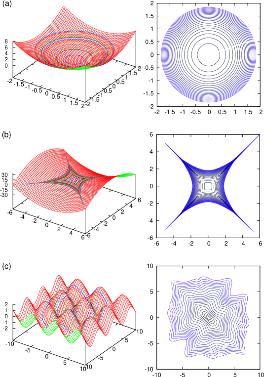
Figure 3: Examples of use of our numerical algorithm to obtain balls with increasing sizes for deterministic metrics. In all cases, and in order to enhance visualization, the metrics have been extracted from the first fundamental form of a simple surface: (a) Paraboloid $z=x^{2}+y^{2}$, a surface with positive curvature; (b) saddle $z=x^{2}-y^{2}$, a surface with negative curvature; (c) egg-crate surface $z(x,y)=\sin(x)+\sin(y)$. Left column shows the balls (solid lines) immersed in the corresponding surfaces. The right column does the same in the Euclidean $(x,y)$ plane.

Generation of a random metric tensor field is performed by assuming that the correlation length is shorter than the cutoff distance assumed for the ball, i.e., $r_{0}<l_{0}$. Thus, the metric tensors at sampled points are statistically independent. The procedure does not require derivatives of the metric tensors, as it would if one insisted on tracking individual geodesics. The metric tensor at each point is specified by providing the two orthogonal unitary eigenvectors, $\vec{v}_{1}$ and $\vec{v}_{2}$, and the two corresponding eigenvalues. Thus, $\vec{v}_{1}$ is generated randomly, $\vec{v}_{2}$ is just chosen to be orthogonal to it, and the eigenvalues are uniform deviates in the interval $[\lambda_{0},\lambda_{1}]$, where $\lambda_{0}$ should be strictly larger than zero.

The balls are analyzed from the Euclidean point of view: Their roughness $W$ is found after fitting to an Euclidean circle, and by computing the average squared deviation from the ball points to it, ultimately averaging over disorder realizations. We will also consider the standard deviation $\sigma_{r}$ of the radius of the fitting Euclidean circle over realizations of the disorder [40]. Thus, $W$ can be interpreted to quantify intra-sample radial fluctuations, while $\sigma_{r}$ assesses inter-sample radial fluctuations.

4 Balls and geodesics in random metrics

The algorithm described in the previous section has been applied to integrate equation (1) numerically for different realizations of the random geometry. Our simulations start with a very small ball, with initial radius $0.05$, and propagate it through a random metric with eigenvalues $\lambda\in[1/20,1]$. The time-step used is $\Delta t=5\cdot 10^{-3}$ and the ultraviolet cutoff interval for the simulation is chosen to be $[l_{0},l_{1}]=[0.01,0.05]$. Scaling results were checked to remain unchanged for smaller values of the discretization parameters.

Figure 4 shows an example of balls with increasing radii for times (i.e., $g$-radii) in the range $t=0.2$ to $3.4$.

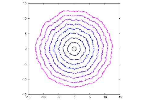
Figure 4: Example of balls of increasing radii of a metric chosen randomly with eigenvalues $\lambda\in[1/20,1]$. The times or $g$-radii grow linearly from $t=0.2$ to $3.4$.

4.1 Roughness

We have simulated equation (1) for 1280 realizations of the disorder in the metric and analyzed the Euclidean roughness of the resulting balls as a function of time (i.e., $g$-radius). The results for the roughness $W(t)$ are shown in figure 5. The figure also shows the time evolution of the standard deviation of the average fitting Euclidean radius, $\sigma_{r}$. Both observables are seen to follow power-law behavior. Thus, $W\sim t^{\chi}$, with $\chi\simeq 1/3$ ($0.333\pm 0.001$). The correspondence between the $\chi$ exponent of random geometry and the $\beta=1/3$ value which characterizes the KPZ universality class is evident.

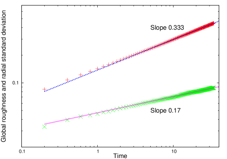
Figure 5: Log-log plot of Euclidean radial roughness $W$ ($+$) and standard deviation $\sigma_{r}$ ($\times$) as functions time (i.e., $g$-radius). Lines correspond to simple power-law behaviors, with exponent values as given in the corresponding labels.

With respect to the sample-to-sample standard deviation of the average Euclidean radii, $\sigma_{r}$, we also obtain a clear power-law, as illustrated in fig. 5, but with a different exponent value, namely, $\sigma_{r}\sim t^{\tilde{\chi}}$, with $\tilde{\chi}=0.17\pm 0.01$. An heuristic argument shows that this value is actually also compatible with KPZ scaling. Indeed, let us assume (1) that the radius grows linearly in time and (2) that the correlation length scales as $\ell\sim t^{1/z}$, with $z=3/2$, as expected within KPZ universality. Then, the number of independent patches on a single droplet will scale as $n_{P}\sim r/\ell\sim t/t^{1/z}=t^{1/3}$. The sample-to-sample standard deviation should then scale as the local fluctuations divided by the square root of the number of patches, $W/\sqrt{n_{P}}\sim t^{1/3}/t^{1/6}=t^{1/6}$. Our value for $\tilde{\chi}$ is compatible with this prediction.

4.2 Geodesic fluctuations

Our next numerical experiment addresses the average lateral deviation of the minimizing geodesics. We define such a geodesic fluctuation in the following way. Consider two points which are an Euclidean distance $L$ apart. Find the minimizing geodesic joining them, and mark also its middle point $M$, see figure 6.

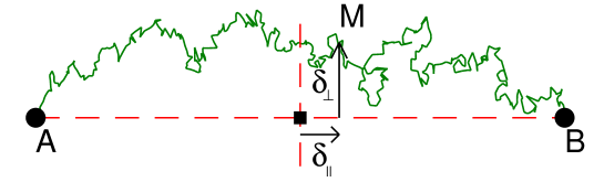
Figure 6: Minimizing geodesic (solid line) between points $A$ and $B$, which are an Euclidean distance $L$ apart. Let $M$ be the middle point in the geodesic, i.e., the point along it which can be reached in the same time from $A$ and from $B$. Then, $\delta_{\perp}$ and $\delta_{\parallel}$ are the lateral and longitudinal deviations between $M$ and the middle point (square) of the straight segment (dashed horizontal line) joining $A$ and $B$. In other terms, they constitute the lateral and longitudinal deviations of the actual geodesic from its Euclidean counterpart.

The coordinates of point $M$ relative to the middle point of the straight segment joining $A$ and $B$, namely $(\delta_{\parallel},\delta_{\perp})$, are, respectively, the longitudinal and lateral fluctuations of the actual geodesic from its Euclidean counterpart. Notice that the disorder averages of both $\delta_{\parallel}$ and $\delta_{\perp}$ should be zero, but their fluctuations are highly informative. According to previous work [13, 14], they are conjectured to scale as $\delta_{\parallel}\sim L^{\chi}$, with the same exponent as the roughness, $\chi=1/3$, and $\delta_{\perp}\sim L^{\xi}$, with $\xi=2/3$, a second critical exponent.

We have estimated both $\delta_{\perp}$ and $\delta_{\parallel}$, fixing points $A,B$ at $(\mp L/2,0)$, for different values of $L$ and 128 realizations of the disorder. Our procedure is as follows: Two balls centered at these points are grown simultaneously. Growth is arrested when both balls intersect for the first time. The coordinates of their first intersection point are, precisely, $M=(\delta_{\parallel},\delta_{\perp})$; see figure 7 (left) for an illustration. The rationale is as follows. Let us call $t_{x}$ the time ($g$-radius) at which both balls first intersect. Point $M$ can be reached in time $t_{x}$ both from $A$ and from $B$, hence it should belong to the minimizing geodesic connecting both points.

In order to save simulation time, each simulation is carried out in practice as follows: We start with two very small balls separated by a small distance $L_{0}$, and grow them until they first intersect. At this moment, we take note of the coordinates of the intersection point, increase the separation of the balls by $\Delta L$, rotate each one by a random angle, and continue the simulation until they intersect again. This procedure is repeated until the desired range for $L$ has been covered. The random rotation ensures that the ensuing intersection points are uncorrelated.

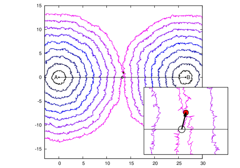
Figure 7: Left: Illustration of the procedure to find the geodesic fluctuations. Balls are grown simultaneously from points $A$ and $B$. Their first intersection point is marked (solid bullet). The vector going from the midpoint on the segment that joins the two ball centers (empty circle) to the intersection point has components $\delta_{\parallel}$ and $\delta_{\perp}$, see inset for a zoomed image. Right: Root-mean-square deviation of the intersection of the balls growing from two points at a distance $L$, in logarithmic scale, for $128$ samples. The lateral fluctuation ($\times$) scales as $\delta_{\perp}\sim L^{\xi}$, with $\xi=0.68\pm 0.02$. The longitudinal fluctuation ($+$) scales as $\delta_{\parallel}\sim L^{\chi}$, with a smaller exponent $\chi=0.36\pm 0.02$. The lines provide power-law fits using these exponent values.

We obtain the root-mean-square horizontal and vertical deviations of the intersection point as functions of the Euclidean distance between the two points. The results appear in figure 7. The lateral fluctuations of the geodesics scale with the separation $L$ between the ball centers as $\delta_{\perp}\sim L^{\xi}$, with $\xi\simeq 2/3$, while the longitudinal fluctuations scale with the same exponent value as the roughness, namely, $\delta_{\parallel}\sim L^{\chi}$, with $\chi\simeq 1/3$. It is straightforward to understand the exponent for the longitudinal fluctuations, as $\delta_{\parallel}$ is quite naturally expected to grow with the ball roughness. Through the rough interface interpretation mentioned above [15], the lateral fluctuations $\delta_{\perp}$, are otherwise related to the increase in the correlation length characteristic of systems in the KPZ universality class, namely, $\delta_{\perp}(t)\sim\ell(t)\sim t^{1/z}$, with $1/z=2/3$. Indeed, the exponent values we obtain for the random metrics system are compatible, within statistical uncertainties, with the so-called Galilean relation, $\chi+1=2\xi$ or, equivalently, $\beta+1=2/z$, which is a hallmark of the KPZ universality class. The geometrical interpretation of this exponent identity within the latter context is the expression, under the scaling hypothesis, of the fact that on average the rough interface grows with uniform speed along the local normal direction [15], implementing a Huygens principle as discussed above.

4.3 Rightmost point statistics

We have experimented with a different approach to find the scaling exponents. For each interface, we find the rightmost point, $\vec{P}$, to be the point with highest $x$-coordinate. If the interface was a circumference, we would have $\vec{P}=(R,0)$, where $R$ is the expected value of the radius. Let us write the deviations as $\vec{P}=(R+\rho_{\parallel},\rho_{\perp})$, with $\rho_{\parallel}$ and $\rho_{\perp}$ having similar interpretations to those discussed for $\delta_{\parallel}$ and $\delta_{\perp}$ in the previous section. Of course, there is nothing special with the $x$-axis, one may choose any direction. A useful strategy is to perform several random rotations of the interface and find the rightmost extreme point for each of them, computing the root mean square values for $\rho_{\parallel}$ and $\rho_{\perp}$. Figure 8 shows the results of this procedure as a function of the average radius size for 1280 realizations, with 50 random directions for each profile. The results are extremely clean: $\rho_{\parallel}\sim R^{\beta}$ with $\beta=0.333\pm 0.001$ and $\rho_{\perp}\sim R^{1/z}$ with $1/z={0.665\pm 0.001}$, fully compatible with KPZ scaling if we consider that $R\sim t$.

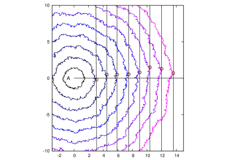
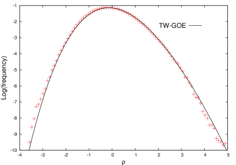
Figure 8: Upper left: Illustration of the rightmost-point procedure to estimate the transverse and longitudinal fluctuations of our interfaces. For each curve, the open symbol corresponds to its right-most point. Upper right: Scaling of the fluctuations with the average radius for each time, using 1280 noise realizations and 50 different rotations per sample. Bottom: full probability distribution for the (rescaled) horizontal position of the rightmost-point, $\delta_{\parallel}$, to have zero mean and variance one. Comparison is provided to the TW-GOE distribution with the same normalization.

Furthermore, we have studied also the full probability distribution for this $\delta_{\parallel}$, as shown in the bottom panel of Fig. 8. The distribution follows a Tracy-Widom type form, but not for the GUE as it is the case for circular fluctuations, but for the GOE. Indeed, the numerical values for skewness and kurtosis are 0.293 and 0.175, fully compatible with the TW-GOE values (0.29346 and 0.16524). This result is analogous to those obtained when considering the extreme-value statistics of the height of curved interfaces in e.g. experiments on turbulent liquid crystals [41] or in the Polynuclear Growth Model [42], see additional references in [41].

5 Radial fluctuations

As discussed in the introduction, physical systems for which fluctuations belong to the 1D KPZ universality class are consistenly being found to not only share the values of the critical exponents $\beta$ and $1/z$ (respectively, $\chi$ and $\xi$ in the random metrics language), but also to be endowed with a larger universality trait, alike to a central limit theorem: Radial fluctuations of the interface follow the same probability distribution function as the largest eigenvalues of large random matrices extracted from the Gaussian unitary ensemble (GUE), i.e., the Tracy-Widom GUE (TW-GUE) distribution. Moreover, higher-order correlations are also conjectured to be part of the universality class, constituting the so-called Airy-2 process [22, 23].

Figure 9 characterizes the probability distribution function of the fluctuations in the Euclidean distances to the origin of points on balls, for different times (or $g$-radii). We consider 171 different values of time $t_{i}$, separated by $0.2$ units, up to $t_{max}=35$ and discarding the first few times. For each time, the corresponding ball is approximated by a circle with radius $r(t)$, which in turn is fit to the deterministic shape $r(t)=r_{0}+vt$. An average over 1280 noise realizations is made. Once such a deterministic contribution to radial growth is identified, we subtract it from the distance to the origin $r_{i}$ of each point on the corresponding ball, as

$$\rho_{i}\equiv{r_{i}-r_{0}-vt\over\Gamma t^{\gamma}},$$ (2)

where $\Gamma$ is a normalization constant. The Prähofer-Spohn conjecture [33, 34] for the radial fluctuations $\rho_{i}$ within the KPZ universality class is that $\gamma$ should be equal to $\beta=1/3$, with a pdf which converges for long times to the TW-GUE distribution. Figure 9 (left) shows the evolution of the third and fourth cumulants of the distribution of radial fluctuations. They both can be seen to approach asymptotically their TW-GUE values, which are, respectively, $0.224$ and $0.093$ [33, 34]. Within our statistics, the decay rates for the differences between our estimates for skewness and kurtosis and their asymptotic values are compatible with power-law rates $t^{-2/3}$ and $t^{-4/3}$, respectively, see the inset of the left panel in figure 9. For the skewness, this convergence rate seems to agree with results in e.g. some discrete growth models [44] and in experiments [41], while this is not the case for the kurtosis. Although further studies are needed, these finite time corrections to the distribution seem likely not to be universal; see additional results e.g. in [45]. Considering the full histogram of the fluctuations, its time evolution is shown on the right panel of figure 9, wherein steady convergence to the TW-GUE distribution can be readily appreciated.

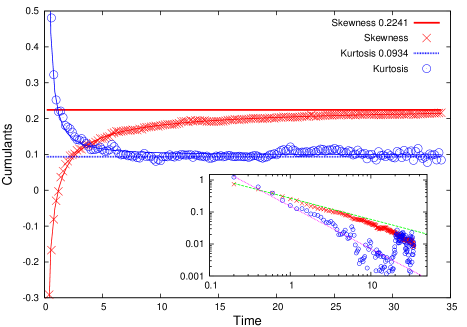
Figure 9: Left: Cumulants [skewness ($\times$) and excess kurtosis ($\circ$)] of the distribution of fluctuations in the Euclidean distances to the origin of points of balls as functions of time (i.e., $g$-radius). As references, the horizontal lines provide the asymptotic values corresponding to the TW-GUE distribution. Convergence is in the form of power-laws (solid curves), approximately $t^{-2/3}$ for the skewness and $t^{-4/3}$ for the kurtosis. The inset is a log-log representation of the same data, in which the latter rates are shown as the green dashed and pink dotted lines, respectively. Right: Full histogram of the rescaled fluctuations in Euclidean distances to the origin, $\rho_{i}$, equation (2), for times as in the legend (symbols). Consistent with the evolution of their cumulants, the distributions are seen to approach the TW-GUE pdf (solid line).

But the Airy-2 process involves more than the single-point fluctuations. In particular, the angular two-point correlation function can also be predicted. For a fixed time $t$, let $r(\theta,t)$ be the maximal radius at a given polar angle $\theta$ for the ball corresponding to $g$-radius equal to $t$. Then, we define the correlator as

$$C(\theta,t)\equiv\left<r(\theta_{0},t)r(\theta_{0}+\theta,t)\right>-\left<r\right>^{2}.$$ (3)

In our simulations, see figure 10, we have found that the two-point functions obtained for different times collapse into an universal curve through

$$u(t)C(\theta,t)\approx g_{2}(v(t)\theta),$$ (4)

where the scaling function, $g_{2}$, is the covariance of the Airy-2 process [46, 26, 47, 29]. The $u(t)$ and $v(t)$ factors have been found numerically through the collapse of the two-point data, and their values are plotted on the right panel of figure 10, showing that

$$u(t)=A_{u}t^{-2/3},\qquad v(t)=A_{v}t^{1/3},$$ (5)

where $A_{u,v}$ are constants. The $v(t)\sim t^{1/3}$ dependence of the rescaled angular variable is related to the growth of the correlation length in a straightforward way: a length variable would require a scaling factor given by $t^{-1/z}=t^{-2/3}$. But since $\theta$ is an angle and the radius scales linearly in time, the scaling factor is modified to $t^{1-1/z}=t^{1/3}$. As seen in fig. 10, convergence to the covariance of the Airy-2 process is indeed obtained for sufficiently long times.

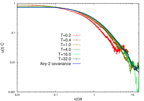
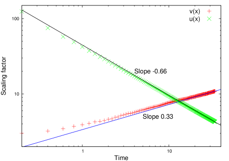
Figure 10: Left: Data collapse of the angular correlation functions $C(\theta,t)$ for different times, to the Airy-2 covariance $g_{2}$, as in eq. 4. Right: Time evolution of the $u(t)$ and $v(t)$ factors employed for the collapse in the left panel, showing power-law behavior as described in eq. 5, namely, $u(x)\sim t^{-2/3}$ and $v(t)\sim t^{1/3}$.

6 Time of arrival

As mentioned in the introduction, first passage percolation (FPP) systems bear a strong relation to the random metric problem studied here [13]. Indeed, the random passage times between neighboring sites can be considered to constitute a discretization of a Riemannian metric. The most important observable in FPP studies is typically the time of arrival to different sites in the lattice, which can be associated to the length of the minimizing geodesic joining the origin to the given point [10, 38, 19].

Measuring times of arrival within our scheme requires a special simulation device, illustrated in figure 11. A number of checkpoints $X_{j}$ have been scattered throughout the manifold. At each time step, a winding-number algorithm is performed in order to check whether each one of them is inside or outside the corresponding ball. When point $X_{j}$ changes status from outside to inside, we identify that time as its arrival time. The points $X_{j}$ are distributed as a linear golden spiral, i.e., their Euclidean radii increase linearly, but their angles follow the sequence $\alpha_{j}=2\pi j\phi$, where $\phi$ is the golden section, $\phi=(\sqrt{5}-1)/2$. This distribution is chosen so as to ensure a uniform angular distribution, as uncorrelated as possible.

Figure 11: Illustration of the checkpoint distribution employed in our algorithm to measure the time of arrival in the random metric system.

The numerical simulations give the expected results, namely, the times of arrival grow linearly with distance to the origin, and their standard deviation also increases with distance, as $\sigma_{t}\sim d^{0.339}$, see figure 12 (upper left panel). The higher cumulants are compatible with the TW-GUE distribution, averaging to $-0.218$ for the skewness and 0.078 for the kurtosis, see upper right panel. These values are to be compared with those obtained in [33, 34], $-0.224$ and $0.093$, respectively, as in the case of the radial fluctuations studied earlier in fig. 9. The full histogram of arrival times, and its comparison with the TW-GUE distribution, is shown in figure 12 (lower panel). Excellent agreement is obtained.

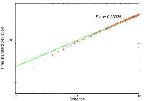
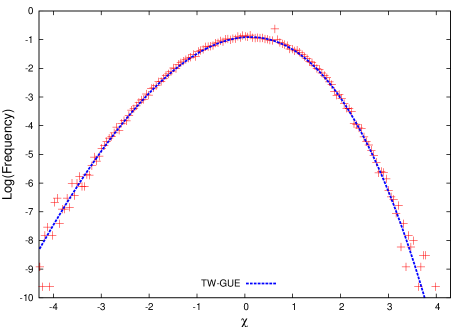
Figure 12: Numerical results for the distribution of times of arrival in the random metrics system. Top-left: Deviation of the time of arrival ($+$) as a function of Euclidean distance to the center of the ball. The slope of the straight line is provided in the legend. Top-right: Cumulants [skewness ($\times$) and kurtosis ($\Box$)] of the time distribution of arrival times as a function of the Euclidean radius. Exact TW-GUE values are given by the horizontal straight lines, for reference. Bottom: Histogram of the time of arrival fluctuations ($+$), and comparison with the TW-GUE distribution (dashed line).

7 Conclusions and further work

We have shown evidence of KPZ scaling in a purely geometric model, in which the role of the evolving interface is played by balls of increasing radii in a random manifold. Universal behavior occurs at distances which are large as compared to either the correlation or the curvature lengths. When the balls on the random manifold are viewed from an Euclidean point of view, they appear to be rough. If the radius of the balls is thought of as time, we show that the growth of the Euclidean roughness of the ball is $W\sim t^{\chi}$, with $\chi=1/3$. Moreover, study of the minimizing geodesics has shown that the lateral correlations of the fluctuations in the balls scale as $\ell\sim t^{\xi}$ with $\xi=2/3$. These critical exponent values are the hallmark of the KPZ universality class, although in a different language, namely, $\chi\to\beta$ and $\xi\to 1/z$. Our results thus allow to assess numerically the predictions for Riemannian first-passage percolation [13, 14], providing a detailed picture of its stochastic behavior. Given the relation to FPP proper, this detailed description may aid in the development of rigorous proofs that fully justify the values of the wandering and fluctuation exponents in this important discrete model.

In principle, the results we obtain may come as a surprise. The random geometry model we study features quenched disorder, i.e., the disorder does not change with time. However, we obtain standard KPZ universality (namely, the critical behavior corresponding to time-dependent noise), which differs from the so-called quenched-KPZ universality class [16]. The latter describes the scaling behavior of e.g. the quenched KPZ equation, in which a depinning transition occurs: If the intensity of the external driving $F$ is below a finite threshold $F_{c}$, then the average interface velocity $v$ is zero. On the contrary, the interface moves with a non-zero $v$ for $F>F_{c}$. Actually, for sufficiently large $F$ the quenched disorder is somehow seen by the interface as time-dependent noise, and the scaling behavior becomes standard KPZ [16]. Quenched-KPZ scaling applies at the depinning threshold $F=F_{c}$ [48]. In the model we study the average interface velocity is non-zero by construction, so that one is always in the moving phase, in such a way that seemingly only standard KPZ behavior ensues. Given the relation of the random geometry model with FPP, and in turn the connection of the latter with the Eden model, it is natural to ponder whether our results may provide some clue on the relation between the quenched and the time-dependent KPZ universality classes. Note that TW fluctuations have been also found in other paradigmatic systems of quenched disorder, such as spin glasses, structural glasses, or the Anderson model [49, 50]. This point seems to warrant further study.

Actually, TW statistics do appear in our model both in the Euclidean fluctuations of the random balls and in the random-metric fluctuations of the Euclidean balls, which can be described as fluctuations in the arrival times at different distances from the origin. Again the deviation of these values follows the same power-law as the roughness in standard KPZ growth, namely, $\sigma_{t}\sim t^{\chi}$, with $\chi=1/3$, and the fluctuations follow TW statistics. Due to the wide connections and applications of the FPP model to disordered systems, one can speculate whether this reinterpretation might allow to unveil TW statistics in still many other phenomena in which it has not been identified yet. This would strengthen the role of TW fluctuations as a form of a central limit theorem for many far-from-equilibrium phenomena.

The code used to carry out the simulations in this work has been uploaded as free software to a public repository [51].

References

References

- [1] R. Adler and J. Taylor, Random fields and geometry, Springer (2007).
- [2] C. Itzykson and J.-M. Drouffe, Statistical Field Theory, Cambridge University Press (1991).
- [3] B. Booß-Bavnbek, G. Esposito and M. Lesch, New paths towards quantum gravity, Springer (2009).
- [4] D. Nelson, T. Piran and S. Weinberg, Statistical Mechanics of Membranes and Surfaces World Scientific, Singapore (2004).
- [5] D. H. Boal, Mechanics of the cell, Cambridge University Press (2012).
- [6] J. Ambjørn, B. Durhuus and T. Jonsson, Quantum Geometry: A Statistical Field Theory Approach, Cambridge University Press (1997).
- [7] V. Knizhnik, A. M. Polyakov and A. B. Zamolodchikov, Mod. Phys. Lett. A 03, 819 (1988).
- [8] J. M. Hammersley and D. J. A. Welsh, “First-passage percolation, subadditive processes, stochastic networks and generalized renewal theory”, in Bernoulli, Bayes, Laplace anniversary volume, J. Neyman and L. M. LeCam eds., Springer-Verlag (1965), p. 61.
- [9] C. D. Howard, “Models of first passage percolation”, in Probability on discrete structures, H. Keston ed., Springer (2004), p. 125.
- [10] H. Kesten, Prog. in Probability 54, 93 (2003).
- [11] M. Eckhoff, J. Goodman, R. van der Hofstad and F. R. Nardi, J. Stat. Phys. 151, 1056 (2013).
- [12] M. E. J. Newman, Networks: An Introduction, Oxford University Press (2010).
- [13] T. LaGatta and J. Wehr, J. Math. Phys. 51, 053502 (2010).
- [14] T. LaGatta and J. Wehr, Comm. Math. Phys. 327, 181 (2014).
- [15] J. Krug and H. Spohn, “Kinetic Roughening of Growing Surfaces”, in Solids Far from Equilibrium, C. Godrèche ed., Cambridge University Press (1992), p. 479.
- [16] A.-L. Barabási and H. E. Stanley, Fractal Concepts in Surface Growth, Cambridge University Press (1995).
- [17] J. Krug, Adv. Phys. 46, 139 (1997).
- [18] M. Kardar, G. Parisi and Y.-C. Zhang, Phys. Rev. Lett. 56, 889 (1986).
- [19] S. Chatterjee, Ann. Math. 177, 663 (2013).
- [20] A. Auffinger and M. Damron, Ann. Probab. 42, 1197 (2014).
- [21] K. A. Takeuchi, M. Sano, T. Sasamoto and H. Spohn, Sci. Rep. 1, 34 (2011).
- [22] M. Prähofer and H. Spohn, J. Stat. Phys. 108, 1071 (2002).
- [23] I. Corwin, J. Quastel and D. Ramenik, Comm. Math. Phys. 317, 347 (2013).
- [24] I. Corwin, Random Matrices: Theor. Appl. 1, 1130001 (2012).
- [25] S. D. Alves, T. J. Oliveira and S. C. Ferreira, Europhys. Lett. 96, 48003 (2011).
- [26] T. J. Oliveira, S. C. Ferreira and S. G. Alves, Phys. Rev. E 85, 010601(R) (2012).
- [27] K. A. Takeuchi and M. Sano, Phys. Rev. Lett. 104, 230601 (2010).
- [28] P. J. Yunker, M. A. Lohr, T. Still, A. Borodin, D. J. Durian and A. G. Yodh, Phys. Rev. Lett. 110, 035501 (2013); ibid 111 209602 (2013).
- [29] M. Nicoli, R. Cuerno and M. Castro, Phys. Rev. Lett. 111, 209601 (2013).
- [30] T. Sasamoto and H. Spohn, Phys. Rev. Lett. 104, 230602 (2010).
- [31] G. Amir, I. Corwin and J. Quastel, Comm. Pure Appl. Math. 64, 466 (2011).
- [32] P. Calabrese and P. Le Doussal, Phys. Rev. Lett. 106, 250603 (2011).
- [33] M. Prähofer and H. Spohn, Phys. Rev. Lett. 84, 4882 (2000).
- [34] M. Prähofer and H. Spohn, Physica A 279, 342 (2000).
- [35] K. Johansson, Comm. Math. Phys. 209, 437 (2000).
- [36] V. S. Dotsenko, J. Stat. Mech.: Theory Exp. 2010, P07010 (2010).
- [37] K. A. Takeuchi, J. Stat. Mech.: Theory Exp. 2012, P05007 (2012).
- [38] K. Johansson, Comm. Math. Phys. 209, 437 (2000).
- [39] J. Rodriguez-Laguna, S. N. Santalla and R. Cuerno, J. Stat. Mech.: Theory Exp. 2011, P05032 (2011).
- [40] S. N. Santalla, J. Rodriguez-Laguna and R. Cuerno, Phys. Rev. E 89, 010401(R) (2014).
- [41] K. A. Takeuchi and M. Sano, J. Stat. Phys. 147, 853 (2012).
- [42] K. Johansson, Comm. Math. Phys. 242, 277 (2003).
- [43] K. Burns and M. Gidea, Differential Geometry and Topology: with a view to dynamical systems, CRC Press, Boca Ratón (2005).
- [44] P. L. Ferrari and R. Frings, J. Stat. Phys. 144, 1123 (2011).
- [45] S. G. Alves, T. J. Oliveira and S. C. Ferreira, J. Stat. Mech. Theory Exp. 2013, P05007 (2013).
- [46] S. G. Alves, T. J. Oliveira and S. C. Ferreira, Europhys. Lett. 96, 48003 (2011).
- [47] F. Bornemann, Math. Comput. 79, 871 (2010).
- [48] L.-H. Tang and H. Leschhorn, Phys. Rev. A 45, R8309 (1991); H. Leschhorn, Phys. Rev. E 54, 1313 (1996).
- [49] M. Castellana, A. Decelle and E. Zarinelli, Phys. Rev. Lett. 107, 275701 (2011); M. Castellana, Phys. Rev. Lett. 112, 215701 (2014).
- [50] A. M. Somoza, M. Ortuño and J. Prior, Phys. Rev. Lett. 99, 116602 (2007).
- [51] http://github.com/jvrlag/riemann.