On the possible observational signatures of white dwarf dynamical interactions

Abstract

We compute the possible observational signatures of white dwarf dynamical interactions in dense stellar environments. Specifically, we compute the emission of gravitational waves, and we compare it with the sensitivity curves of planned space-borne gravitational wave detectors. We also compute the light curves for those interactions in which a detonation occurs, and one of the stars is destroyed, as well as the corresponding neutrino luminosities. We find that for the three possible outcomes of these interactions — which are the formation of an eccentric binary system, a lateral collision in which several mass transfer episodes occur, and a direct one in which just a single mass transfer episode takes place — only those in which an eccentric binary are formed are likely to be detected by the planned gravitational wave mission eLISA, while more sensitive detectors would be able to detect the signals emitted in lateral collisions. On the other hand, the light curves (and the thermal neutrino emission) of these interactions are considerably different, producing both very powerful outbursts and low luminosity events. Finally, we also calculate the X-ray signature produced in the aftermath of those interactions for which a merger occurs. We find that the temporal evolution follows a power law with the same exponent found in the case of the mergers of two neutron stars, although the total energy released is smaller.

1 Introduction

Close encounters of two white dwarfs in dense stellar environments, as the central regions of galaxies or the cores of globular clusters, are interesting phenomena that have several potential applications, and hence deserve close scrutiny. This type of interactions can be the result of either a serendipitous approach due to the high stellar density of the considered stellar system or the result of the interaction of a binary system containing a white dwarf with a third star in a triple system, via the Kozai-Lidov mechanism — see Kushnir et al. (2013) for a detailed description of this scenario. Nevertheless, the details of how the intervening white dwarfs are brought close enough to experience such dynamical interactions do not play an important role in the result of the interaction, so the outcome of the interaction is independent of these details, and the gross features of the hydrodynamical evolution are totally general.

Among the possible applications of these interactions we mention that it has been shown (Rosswog et al., 2009) that head-on collisions of two white dwarfs is a viable mechanism to produce Type Ia Supernovae (SNIa), one of the most energetic events in the Universe. This, in turn, has obvious implications in Cosmology, as SNIa are one of the best distance indicators. However, there are situations in which the two white dwarfs interact but the interaction does not result in a powerful thermonuclear outburst leading to the complete disruption of the two stars, whereas in some other the release of nuclear energy is very modest, and finally there are other cases in which no nuclear energy is released at all. Specifically, it has been recently shown (Aznar-Siguán et al., 2013) that white dwarf close encounters can have three different outcomes, depending on the initial conditions of the interaction – namely, the initial energy and angular momentum of the pair of white dwarfs, or equivalently the impact parameter and initial velocity of the pair of stars. In particular, these interactions can lead to the formation of an eccentric binary system, to a lateral collision in which several mass transfer episodes between the disrupted less massive star and the more massive one occur, and finally to a direct collision, in which only one catastrophic mass transfer event occurs. Additionally, it turns out that for these two last outcomes there is a sizable region of the parameter space for which the conditions for a detonation to occur are met, leading in some cases to the total disruption of both white dwarfs, and to a large dispersion of the nuclear energy released during the interaction.

According to the above mentioned considerations, during the last few years the close encounters of two white dwarfs is a research topic that has been the subject of renewed interest. Specifically, the dynamical behavior of these interactions has been simulated by Rosswog et al. (2009), Raskin et al. (2009), Lorén-Aguilar et al. (2010), Raskin et al. (2010), Hawley et al. (2012), Aznar-Siguán et al. (2013) and Kushnir et al. (2013). It is to be noted that in almost all the cases the simulations were carried out using Smoothed Particle Hydrodynamics (SPH) codes, given the intrinsic difficulties of simulating these encounters on an Eulerian grid. Nevertheless, most of these simulations have focused on the head-on collisions of two white dwarfs, and the only works in which a systematic and comprehensive study of the effects of the initial conditions on the result of these interactions was done are those of Lorén-Aguilar et al. (2010) and Aznar-Siguán et al. (2013). In particular, Lorén-Aguilar et al. (2010) studied the dynamical interactions of two otherwise typical white dwarfs, of masses $0.6\,M_{\sun}$ and $0.8\,M_{\sun}$, for a reduced set of energies and angular momenta. Later on, Aznar-Siguán et al. (2013) extended the previous work, studying a significantly broader range of initial conditions for a larger set of white dwarf masses and core chemical compositions, including helium, carbon-oxygen, and oxygen-neon white dwarfs.

The study of Aznar-Siguán et al. (2013) demonstrated that the masses of ⁵⁶Ni synthesized in the strongest dynamical interactions can vary by orders of magnitude, and so do the typical luminosities. Actually, the mass of ⁵⁶Ni obtained in the several sets of simulations performed so far, and thus the corresponding luminosities, range from those typical of macro-nova events, to sub-luminous and super-luminous supernova events. Nonetheless, it is important to realize that the spread in the mass of ⁵⁶Ni produced during the most violent phases of the most energetic interactions does not only depend on the adopted initial conditions but also, as shown by Aznar-Siguán et al. (2013) and Kushnir et al. (2013), on the adopted prescription of the artificial viscosity, and on the resolution employed in the simulations, among other (less important) factors. Additionally, one has to note that the parameter space of such dynamical interactions is huge and the complexity of the physical mechanism of the interactions is extremely high. Aznar-Siguán et al. (2013) chose to account for the first point by producing a vast set of numerical simulations, but this comes of the expense of the second issue. Consequently, most likely the tidal interaction is reasonably captured in moderately-resolved SPH simulations, but combustion processes are possibly not completely well resolved. Nevertheless, although a thorough resolution study is still lacking, the masses of ⁵⁶Ni synthesized in the several independent sets of simulations agree within a factor of $\sim 5$, and the qualitative picture of the hydrodynamical evolution is quite similar in all the cases — see Sect. 5.1 of Aznar-Siguán et al. (2013) for additionail details.

Despite the large efforts invested in modelling these interactions, quite naturally most of them have focused on the dynamics of the events, and on the resulting nucleosynthesis, whilst little attention has been paid to other possible observational signatures. This is in contrast with the considerable deal of work done so far for the case in which two neutron stars merge or collide — see, for instance, (Rosswog et al., 2013), and references therein. In this paper we aim at filling this gap by computing the gravitational waveforms, the corresponding light curves for those events in which some ⁵⁶Ni is synthesized, the associated emission of neutrinos, and the X-ray luminosity of the fallback material. All of them individually, or used in combination, would hopefully allow us to obtain useful information about these events.

The emission of gravitational waves in these iteractions should be quite apparent, given that the two interacting white dwarfs are subject to large accelerations, and that in most of the situations there is no symmetry. Although gravitational waves have not been yet detected, with the advent of the current generation of terrestrial gravitational wave detectors and of space-borne interferometers, it is expected that the first direct detections will be possible in a future. In particular, much hope has been placed on the space-based interferometer eLISA, a rescoped version of LISA, which will survey for the first time the low-frequency gravitational wave band (from $\sim$0.1 mHz to $\sim$1 Hz). The timescales of the close encounters of two white dwarfs correspond precisely to this frequency interval. Also, for those events in which an explosive behavior is found it is clear that some information about the dynamical interactions could be derived from the analysis of the light curves. On the other hand, neutrino emission in these events should be noticeable, given the relatively high temperatures achieved during the most violent phases of the interaction ($\sim 10^{9}$ K), and an assessment of their detectability is lacking. Finally, the X-ray luminosity of the fallback material interacting with the disk resulting in the aftermath of the interactions would also eventually help in identifying these events.

The paper is organized as follows. We first discuss the methods employed to characterize the observational signatures of white dwarf close encounters and collisions (Sect. 2). Sect. 3 is devoted to analyze the results of our theoretical calculations. Specifically, in Sect. 3.1 we study the emission of gravitational waves. It follows Sect. 3.2 where we discuss the late-time light curves for those interactions which result in powerful detonations, while in Sect. 3.3 we present the thermal neutrino fluxes and we assess their detectability. In Sect. 3.4, we compute the fallback luminosities produced in the aftermath of those interactions which result in a central remnant surrounded by a disk. Finally, in Sect. 4 we summarize our most relevant results, we discuss their significance, and we draw our conclusions.

2 Numerical setup

In this section we describe how we compute the emission of gravitational waves, the light curves for those events which have an explosive outcome, the neutrino fluxes, and the fallback X-ray luminosity of the remnants, for those cases in which the dynamical interaction is not strong enough to disrupt both stars. All the calculations presented in Sect. 3 are the result of post-processing the SPH calculations of interacting white dwarfs of Aznar-Siguán et al. (2013). Since the results of these calculations is a set of trajectories of a collection of individual particles some of the usual expressions must be discretized. Here we explain how we do this.

2.1 Gravitational waves

We compute the gravitational wave emission in the slow-motion, weak-field quadrupole approximation (Misner et al., 1973). Specifically, we follow closely the procedure outlined in Lorén-Aguilar et al. (2005). Within this approximation the strain amplitudes can be expressed in the following way:

$$h^{\rm TT}_{jk}(t,\textbf{x})=\frac{G}{c^{4}d}\big{(}A_{+}(t,\textbf{x})\textbf{e}_{+\,jk}+A_{\times}(t,\textbf{x})\textbf{e}_{\times\,jk}\big{)}$$ (1)

where $d$ is the distance to the source, and the polarization tensor coordinate matrices are defined as:

$$\textbf{e}_{+\,jk} = \frac{1}{\sqrt{2}}[(\textbf{e}_{x})_{j}(\textbf{e}_{x})_{k}-(\textbf{e}_{y})_{j}(\textbf{e}_{y})_{k}]$$ (2)

$$\textbf{e}_{\times\,jk} = \frac{1}{\sqrt{2}}[(\textbf{e}_{x})_{j}(\textbf{e}_{y})_{k}+(\textbf{e}_{y})_{j}(\textbf{e}_{x})_{k}],$$

and

$$A_{+}(t,\textbf{x})=\ddot{Q}_{xx}-\ddot{Q}_{yy},\;\;\;A_{\times}(t,\textbf{x})=+2\ddot{Q}_{xy}$$ (4)

for $i=0$, and

$$A_{+}(t,\textbf{x})=\ddot{Q}_{zz}-\ddot{Q}_{yy},\;\;\;A_{\times}(t,\textbf{x})=-2\ddot{Q}_{yz}$$ (5)

for $i=\pi/2$, being $i$ the angle with respect to the line of sight. In these expressions $Q$ is the quadrupole moment of the mass distribution.

Since, as already mentioned, we are post-processing a set of SPH calculations and, hence, we deal with an ensemble of $n$ individual SPH particles, the double time derivative of the quadrupole moment is discretized in the following way:

$$\ddot{Q}^{\rm TT}_{jk} \approx P_{ijkl}(\textbf{N})\sum^{n}_{p=1}m(p)[2\textbf{v}^{k}(p)\textbf{v}^{l}(p)$$ (6)

$$+ \textbf{x}^{k}(p)\textbf{a}^{l}(p)+\textbf{x}^{l}(p)\textbf{a}^{k}(p)]$$ (7)

Where $m(p)$ is the mass of each SPH particle, $\textbf{x}(p)$, $\textbf{v}(p)$ and $\textbf{a}(p)$ are, respectively, its position, velocity and acceleration, and

$$P_{ijkl}(\textbf{N}) \equiv (\delta_{ij}-N_{i}N_{k})(\delta_{jl}-N_{j}N_{l})$$ (8)

$$- \frac{1}{2}(\delta_{ij}-N_{i}N_{j})(\delta_{kl}-N_{k}N_{l})$$ (9)

is the transverse-traceless projection operator onto the plane ortogonal to the outgoing wave direction, N,

To assess the detectability of the gravitational waveforms we proceed as follows. For the well defined elliptical orbits, we first accumulate the power of the signal during one year. We then compute the characteristic frequencies and amplitudes, and the signal-to-noise-ratios (SNR) according to Zanotti et al. (2003). These characteristic quantities are given by:

$$h_{\rm c} = \left[3\int_{0}^{\infty}\frac{S_{\rm n}\left(f_{\rm c}\right)}{S_{n}\left(f\right)}\left\langle\left|\tilde{h}\left(f\right)\right|^{2}\right\rangle\,f\,df\right]^{1/2}$$ (10)

$$f_{\rm c} = \left[\int_{0}^{\infty}\frac{\left\langle\left|\tilde{h}\left(f\right)\right|^{2}\right\rangle}{S_{n}\left(f\right)}\,f\,df\right]\left[\int_{0}^{\infty}\frac{\left\langle\left|\tilde{h}\left(f\right)\right|^{2}\right\rangle}{S_{\rm n}\left(f\right)}\,df\right]^{-1}$$ (11)

where

$$\tilde{h}(f)=\int_{-\infty}^{\infty}e^{2\pi ift}\,h(t)\,dt$$ (12)

is the waveform in the frequency domain, and $S_{\rm n}$ is the power spectral density of the detector. After this the root-mean-square strain noise:

$$h_{\rm rms}=\sqrt{fS_{\rm n}(f)}$$ (13)

is computed to obtain the SNR:

$${\rm SNR}=\frac{h_{\rm c}}{h_{\rm rms}(f_{\rm c})}.$$ (14)

For the short-lived signals obtained in lateral collisions, we compute the SNR as in Giacomazzo et al. (2011):

$$\left({\rm SNR}\right)^{2}=4\int_{0}^{\infty}\frac{\left|\tilde{h}\left(f\right)\right|^{2}}{S_{\rm n}\left(f\right)}df,$$ (15)

and we compare the product of the Fourier transform of the dimensionless strains and the square root of the frequency, $\tilde{h}(f)f^{1/2}$, with the gravitational-wave detector noise curve. Finally, for direct collisions we only compute the total energy radiated in the form of gravitational waves, since it is unlikely that these events could be eventually detected.

2.2 Light curves

The observable emission of those events in which some ⁵⁶Ni is synthesized during the interaction is powered completely by its radioactive decay and that of its daughter nucleus, ⁵⁶Co (Colgate & McKee, 1969). Specifically, the ⁵⁶Ni synthesized in the explosion decays by electron capture with a half-life of 6.1 days to ⁵⁶Co, which in turn decays through electron capture (81%) and $\beta^{+}$ decay (19%) to stable ⁵⁶Fe with a half-life of 77 days. The early phase is dominated by the down-scattering and the release of photons generated as $\gamma$-rays in the decays, while at late phases the optical radiation escapes freely. The peak radiated luminosity of SNeIa can be approximated with enough accuracy using the scaling law of Arnett (1979). It is expected to be comparable to the instantaneous rate of energy release by radioactivity at the rise time (Branch, 1992).

To model the light curves in those interactions where sizable amounts of ⁵⁶Ni are produced, we adopt the treatment of Kushnir et al. (2013), which provides a relation between the synthesized ⁵⁶Ni mass and the late-time ($\approx$60 days after peak) bolometric light curve. Within this approach, the late-time bolometric light curve is computed numerically using a Monte Carlo algorithm, which solves the transport of photons, and the injection of energy by the $\gamma$-rays produced by the ⁵⁶Ni and ⁵⁶Co decays. To this end we first map, using kernel interpolation, our SPH data to a three-dimensional cartesian velocity grid, and then we employ the Monte Carlo code of Kushnir et al. (2013).

2.3 Thermal neutrinos

Since the densities reached in all the simulations are smaller than $10^{10}$ g cm^-3, the material is expected to be completely transparent to neutrinos. Moreover, as in a sizable number of close encounters the maximum temperatures are in excess of $10^{9}$ K, copious amounts of thermal neutrinos should be emitted. We thus computed this emission taking into account the five traditional neutrino processes — that is, electron-positron annihilation, plasmon decay, photoemission, neutrino bremsstrahlung, as well as neutrino recombination — using the prescriptions of Itoh et al. (1996).

To assess the possibility of detecting some of the emitted neutrinos we follow closely the prescriptions of Odrzywolek & Plewa (2011) and Kunugise & Iwamoto (2007). Specifically, we compute the number of events that could be eventullay observed in the Super-Kamiokande detector when the source is at a distance $d=1$ kpc. We compute first the neutrino spectral flux:

$$\Phi(E_{\nu},t)=\frac{L}{A\langle E_{\nu}\rangle^{4}}\frac{aE_{\nu}^{2}}{1+\exp^{bE_{\nu}/\langle E_{\nu}\rangle}}$$ (16)

where $L$ is the neutrino luminosity at time $t$, $A=4\pi d^{2}$ is the irradiated area, $\langle E_{\nu}\rangle=3.15137\,T_{\nu}$ is the average neutrino energy at time $t$, $a\simeq 17.3574$ and $b\simeq 3.15137$. The values of $L(t)$ and $T_{\nu}(t)$ are obtained from our SPH simulations. Assuming equipartition of energy between all the emitted neutrino flavors, the number of events detected in a water Cherenkov detector can be approximated by estimating the rate of electron-neutrino neutrino scatterings. The cross section of this scattering depends on the threshold energy of recoil electrons in the experiment, $T^{\rm th}_{\rm e}$:

$$\sigma(E_{\nu},T^{\rm th}_{\rm e}) = \frac{\sigma_{0}}{m_{\rm e}}\Bigg{[}\left(g_{1}^{2}+g_{2}^{2}\right)\left(T_{\rm e}^{\rm max}-T_{\rm e}^{\rm th}\right)$$ (17)

$$- \left(g_{2}^{2}+g_{1}g_{2}\frac{m_{\rm e}}{2E_{\nu}}\right)\left(\frac{T_{\rm e}^{\rm max^{2}}-T_{\rm e}^{\rm th^{2}}}{E_{\nu}}\right)$$

$$+ \frac{1}{3}g_{2}^{2}\left(\frac{T_{\rm e}^{\rm max^{3}}-T_{\rm e}^{\rm th^{3}}}{E_{\nu}^{3}}\right)\Bigg{]},$$

where $\sigma_{0}\simeq 88.06\times 10^{-46}\,{\rm cm}^{2},$

$$T_{\rm e}^{\rm max}=\frac{2E_{\nu}^{2}}{m_{\rm e}+2E_{\nu}}$$

is the maximum kinetic energy of the recoil electron at a neutrino energy $E_{\nu}$, $g_{1}\simeq 0.73$ and $g_{2}\simeq 0.23$. The time-integrated spectra is then

$$F_{\nu}(E_{\nu})=\int\Phi(E_{\nu},t)dt,$$

and the total number of events is:

$$N=nV\int F_{\nu}(E_{\nu})\sigma(E_{\nu},T^{\rm th}_{\rm e})dE_{\nu},$$

where $n$ is the number density of electrons in the water tank and $V$ is its volume. We consider the Super-Kamiokande detector, with a fiducial volume of 22,500 tons.

2.4 Fallback luminosities

Another possible observational signature of these types of collisions and close encounters is the emission of high-energy photons from the fallback material in the aftermath of the interaction. As mentioned, in some cases only one of the stars intervening in the dynamical interaction is disrupted, and its material goes to form a disk orbiting the more massive white dwarf. Most of the material of these disks has circularized orbits. However, it turns out that a general feature of these interactions is that some of the SPH particles of the disk have highly eccentric orbits. After some time this material interacts with the rest of the disk. As shown by Rosswog (2007), the relevant timescale for these particles is not the viscous one, but instead their evolution is set by the distribution of eccentricities. To compute how these particles interact with the newly formed disk, and which are the corresponding fallback accretion luminosities, we follow closely the approach described in Rosswog (2007). That is, we assume that the kinetic energy of these particles is dissipated within the radius of the disk.

3 Results

In this section we present the possible observational consequences of the interactions. The section is organized as follows. We first describe the resulting gravitational waveforms. We do so for the three possible outcomes of the interactions. This is done in Sects. 3.1.1 to 3.1.3. It follows Sect. 3.2 where we present the light curves for those interactions in which a detonation, with the subsequent disruption of one of the stars, occurs, whereas in Sect. 3.3 we discuss the neutrino emission of these interactions. Finally, in Sect. 3.4 we describe the fallback X-ray luminosities for those interactions in which a debris region around a central white dwarf is formed.

3.1 Gravitational wave radiation

3.1.1 Eccentric orbits

Figure 1: Gravitational waveforms for a close encounter in which an eccentric binary is formed. For this particular case both white dwarfs have equal masses, $M=0.8\,M_{\sun}$, whilst the adopted initial conditions are $v_{\rm ini}=200$ km s^-1 and $\Delta y=0.4\,R_{\sun}$. We only show the waveforms $h_{+}$ (top panel) and $h_{\times}$ (bottom panel) for an inclination $i=0^{\circ}$ and a distance of 10 kpc, in units of $10^{-22}$. See text for details.

As mentioned, the most complete and comprehensive study of the close encounters of two white dwarfs is that of Aznar-Siguán et al. (2013), which covers a considerably wide range of masses and chemical compositions of the interacting white dwarfs, as well as of initial conditions. In particular, they characterize the initial conditions in terms of the initial relative velocity ($v_{\rm ini}$) and the initial distance perpendicular to the relative velocity ($\Delta y$) at a sufficiently large distance so that the two interacting white dwarfs are not affected by tidal forces. Here we will compute the gravitational waveforms of the interactions computed by these authors and we will refer to them employing this notation.

Figure 2: Fourier transforms of the gravitational waveforms of Fig. 1, in units of $10^{-23}$.

Table 1: Signal-to-noise ratios of the gravitational waves of the interactions resulting in eccentric orbits, for the case of eLISA, adopting $i=0^{\circ}$ and a distance of 10 kpc.

Run	$M_{1}+M_{2}$	$e$	$f$	SNR
	($M_{\sun}$)		(Hz)
$v_{\rm ini}=150\;\text{km/s}\quad\quad\Delta y=0.4\;R_{\sun}$
55	0.2+0.4	0.736	5.54$\times 10^{-4}$	1.90
56	0.4+0.4	0.799	6.91$\times 10^{-4}$	5.25
$v_{\rm ini}=200\;\text{km/s}\quad\quad\Delta y=0.3\;R_{\sun}$
59	0.2+0.4	0.695	6.64$\times 10^{-4}$	2.00
60	0.4+0.4	0.762	8.64$\times 10^{-4}$	5.87
$v_{\rm ini}=200\;\text{km/s}\quad\quad\Delta y=0.4\;R_{\sun}$
25	0.8+0.6	0.796	9.11$\times 10^{-4}$	16.41
26	0.8+0.8	0.820	1.00$\times 10^{-3}$	23.42
27	1.0+0.8	0.840	1.09$\times 10^{-3}$	30.48
28	1.2+0.8	0.855	1.16$\times 10^{-3}$	37.38
63	0.2+0.4	0.564	4.25$\times 10^{-4}$	0.48
64	0.4+0.4	0.657	5.74$\times 10^{-4}$	2.49
65	0.8+0.4	0.764	8.12$\times 10^{-4}$	9.70
$v_{\rm ini}=300\;\text{km/s}\quad\quad\Delta y=0.3\;R_{\sun}$
29	0.8+0.6	0.705	1.03$\times 10^{-3}$	15.11
30	0.8+0.8	0.736	1.17$\times 10^{-3}$	22.90
31	1.0+0.8	0.762	1.30$\times 10^{-3}$	31.08
32	1.2+0.8	0.783	1.41$\times 10^{-3}$	39.33
67	0.4+0.4	0.571	5.21$\times 10^{-4}$	1.38
68	0.8+0.4	0.666	8.82$\times 10^{-4}$	8.11
69	1.2+0.4	0.737	1.17$\times 10^{-3}$	17.22
$v_{\rm ini}=300\;\text{km/s}\quad\quad\Delta y=0.4\;R_{\sun}$
33	0.8+0.6	0.576	6.64$\times 10^{-4}$	6.04
34	0.8+0.8	0.620	7.67$\times 10^{-4}$	10.71
35	1.0+0.8	0.657	8.62$\times 10^{-4}$	16.90
36	1.2+0.8	0.688	9.49$\times 10^{-4}$	23.77
70	0.8+0.4	0.525	5.51$\times 10^{-4}$	2.99
71	1.2+0.4	0.621	7.67$\times 10^{-4}$	8.05

As previously explained, some of the close encounters computed by Aznar-Siguán et al. (2013) result in the formation of a binary system that survives the interaction and no mass transfer between the two stars occurs. In these cases the eccentricity of the orbit is always large, $e>0.5$. Fig. 1 shows the resulting gravitational dimensionless strains of a typical case, in units of $10^{-22}$, for an edge-on orbit. The two polarizations of the gravitational radiation, $h_{+}$ and $h_{\times}$, are shown, respectively, in the top and bottom panels, for a full period of the orbit. The corresponding dimensionless Fourier transforms, $H(f)=\tilde{h}/T$ where $T=1$ yr, of these gravitational wave patterns are displayed in Fig. 2. As can be seen, the gravitational wave emission presents a single, narrow, large pulse, which occurs at the periastron, whereas the corresponding Fourier transforms, $H_{+}$ and $H_{\times}$, present a peak at the orbital frequency, and several Fourier components at larger frequencies. This was expected, as a binary system in a circular orbit produces a monochromatic gravitational waveform at twice the orbital frequency, while for eccentric orbits it is found — see, for instance, Wahlquist (1987) — that the binary system radiates power at the fundamental mode and at several harmonics of the orbital frequency. The reason for this is clear, since it is at closest approach when the accelerations are larger, thus resulting in an enhanced emission of gravitational radiation. Moreover, it turns out that for a fixed energy, the larger the eccentricity, the smaller the distance at closest approach, and therefore the larger the radiated power.

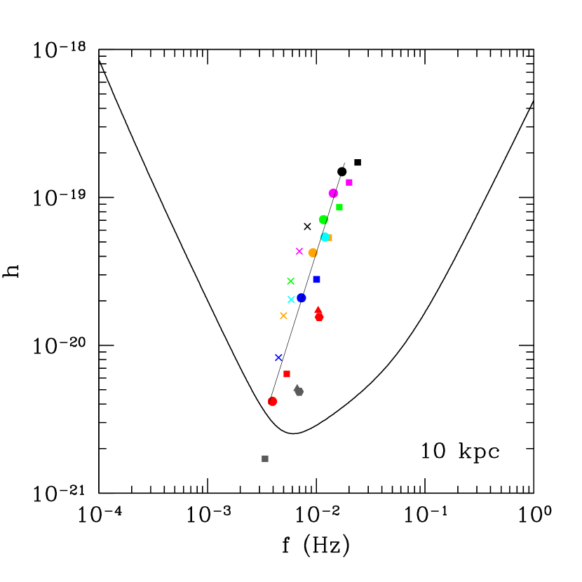
Figure 3: A comparison of the signal produced by the close white dwarf binary systems studied here, when a distance of 10 kpc is adopted, with the spectral distribution of noise of eLISA for a one year integration period, and for a null inclination. We assess the detectability of the $h_{+}$ dimensionless strain. The different colors denote different masses of the interacting white dwarfs, whereas the different symbols are used to distinguish between different initial conditions. Specifically, black symbols correspond to a $1.2\,M_{\sun}+0.8\,M_{\sun}$ binary system, magenta ones to a $1.0\,M_{\sun}+0.8\,M_{\sun}$, green symbols to a $0.8\,M_{\sun}+0.8\,M_{\sun}$, cyan ones to a $1.2\,M_{\sun}+0.4\,M_{\sun}$, orange symbols to a $0.8\,M_{\sun}+0.6\,M_{\sun}$, blue ones to a $0.8\,M_{\sun}+0.4\,M_{\sun}$, red symbols to a $0.4\,M_{\sun}+0.4\,M_{\sun}$, and grey ones are used for a $0.4\,M_{\sun}+0.2\,M_{\sun}$ binary system. On the other hand, hexagons are used for the case in which $v_{\rm ini}=150$ km/s and $\Delta y=0.4\,R_{\sun}$, triangles for $v_{\rm ini}=200$ km/s and $\Delta y=0.3\,R_{\sun}$, squares for $v_{\rm ini}=200$ km/s and $\Delta y=0.4\,R_{\sun}$, circles for $v_{\rm ini}=300$ km/s and $\Delta y=0.3\,R_{\sun}$, crosses for $v_{\rm ini}=300$ km/s and $\Delta y=0.4\,R_{\sun}$. See the on-line edition of the journal for a color version of this figure.

In Table 1 we list for each of the runs of Aznar-Siguán et al. (2013) which result in the formation of an eccentric binary system the masses of the interacting white dwarfs, the eccentricity of the orbit, the frequency of the fundamental mode, and the signal-to-noise ratios for $h_{+}$ for the eLISA mission, adopting $i=0^{\circ}$ and a distance of 10 kpc. Also listed, for the sake of completeness, is the run number (first column) as quoted in Aznar-Siguán et al. (2013). As can be seen, eLISA will be able to detect almost all these systems with sufficiently large SNRs. Only run number 63, which corresponds to the binary system with an orbit with the smallest eccentricity ($e=0.564$) and for which the two interacting white dwarfs have the smallest masses — namely, $M_{1}=0.4\,M_{\sun}$ and $M_{2}=0.2\,M_{\sun}$ — will not be detectable. The rest of the interactions have, in general, large SNRs.

Figure 4: Gravitational waveforms for a close encounter in which the outcome of the interaction is a lateral collision. For this particular case two white dwarfs of masses $0.8\,M_{\sun}$ and $0.6\,M_{\sun}$, respectily, collide. The adopted initial conditions of this interaction are $v_{\rm ini}=200$ km s^-1 and $\Delta y=0.3\,R_{\sun}$. As in Fig. 1 we only show the waveforms $h_{+}$ (top panel) and $h_{\times}$ (bottom panel) for an inclination $i=0^{\circ}$ and a distance of 10 kpc. Again, the units of of the dimensionless stresses are $10^{-22}$.

In Fig. 3 we display the characteristic amplitudes and frequencies of the $h_{+}$ dimensionless strain for $i=0^{\circ}$ and we compare them with the sensitivity curve of eLISA, computed using the analytical approximation of Amaro-Seoane et al. (2013). As previously noted, only run number 63 lies below the eLISA sensitivity limit. Moreover, in this figure it can be clearly seen that for a fixed initial condition — that is for a fixed pair of values of $v_{\rm ini}$ and $\Delta y$ — the characteristic amplitude as well as the frequency decreases with the total mass. The mass ratio of the interacting white dwarfs, $q={M_{2}}/{M_{1}}$, also plays a role. This can be seen when simulations 30 and 69, or 34 and 71, are compared. Both pairs of simulations have the same initial conditions and total mass, but different values of $q$. As can be seen, the value of the characteristic amplitude in runs 69 and 71 — which have $q=1/3$ — is smaller, while the characteristic frequencies are larger than those of runs 30 and 34, respectively — which have $q=1$. Finally, it is interesting to realize that for a given set of initial conditions the runs of different masses lie approximately on straight lines, which are not all shown for the sake of clarity. In particular, we only show, using a thin solid line, the case in which the initial conditions are $v_{\rm ini}=300$ km/s and $\Delta y=0.3\,R_{\sun}$.

3.1.2 Lateral collisions

In lateral collisions the less massive white dwarf is tidally deformed by the more massive star at closest approach to such an extent that in the end some of its material is accreted by the massive companion. This occurs in several mass tranfer episodes, and the resulting final configuration consists of a central compact object surrounded by a hot, rapidly rotating corona, and an external region where some of the debris produced during the dynamical interaction can be found. A typical example of the gravitational wave pattern resulting in these cases is shown in Fig. 4, which corresponds to run number 21 of Aznar-Siguán et al. (2013). This specific simulation corresponds to the dynamical interaction of two white dwarfs with masses $0.8\,M_{\sun}$ and $0.6\,M_{\sun}$, whereas the adopted initial conditions were $v_{\rm ini}=200$ km s^-1 and $\Delta y=0.3\,R_{\sun}$. Again, in this figure we only show the waveforms $h_{+}$ (top panel) and $h_{\times}$ (bottom panel) for an inclination $i=0^{\circ}$ and a distance of 10 kpc, in units of $10^{-22}$. As can be seen, the time evolution of the dimensionless strains presents a series of peaks. For this specific case each one of these peaks corresponds to a mass transfer episode, which occurs short after the passage through the periastron. Nevertheless, it is to be noted that, depending on the masses of the stars and on the initial conditions of the close encounter, the eccentricity of the orbit and the distance at closest approach may be quite different for the several lateral collisions studied here. Hence, the number of periastron passages shows a wide range of variation. However, a general feature in all cases is that the emission of gravitational waves is largest for the first passages through the periastron and the amplitude of the narrow peaks of gravitational wave radiation decreases in subsequent passages. Note as well that the time difference between successive peaks of the gravitational wave pattern also decreases as time passes by. All this is a consequence of the fact that after every passage through the periastron the orbit is slightly modified, either because the less massive white dwarf is substantially deformed by tidal forces in those cases in which during the first passages through the periastron there is no mass transfer from the less massive white dwarf to the more massive one, or because mass transfer has happened, and the orbit becomes less eccentric. In the former case, after a few passages through the periastron mass transfer occurs, and the subsequent evolution is similar to that of lateral collisions in which there is a mass transfer episode during the first closest approach. Finally, after several mass transfers, the binding energy of the less massive star becomes positive and it is totally destroyed, leading to a merger. This causes the sudden decrease of the gravitational wave emission, although some oscillations of the remnant still radiate gravitational waves — in a way very much similar to that of the ring-down phase found in mergers of two compact objects — but with a significantly smaller amplitude than the previous ones.

Figure 5: Fourier transforms of the gravitational waveforms of Fig. 4, in units of $10^{-23}$.

The dimensionless Fourier transform of the gravitational wave pattern shown in Fig. 4 is displayed in Fig. 5. The only difference with those Fourier transforms shown in Fig. 2 is that in this case to compute the dimensionless Fourier transform we adopt the duration of the merger. In contrast with the Fourier transform of the gravitational wave emission presented in Fig. 2, which is discrete because the signal is periodic, now the emission of gravitational waves is characterized by a continuous spectrum, and presents two peaks. The first one is a broad, smooth peak at around $f=3$ mHz, while the second one, which is of larger amplitude but more noisy, occurs at larger frequencies, $\sim 20$ mHz. Since in our numerical configuration all the lateral collisions have orbits which can be well approximated until the passage through the periastron by elliptical ones, the first of these peaks corresponds to the fundamental mode of the eccentric orbit, while the second one is due to the presence of higher order harmonics, as it occurs for the pure elliptical orbits previously analyzed in Sect. 3.1.1, being the most significant difference the continuous shift in frequency due to orbit circularization, which noticeably broadens the fundamental mode.

Table 2: Properties of lateral collisions.

Run	$M_{1}+M_{2}$	$N$	$M_{\rm Ni}$	$E_{\rm GW}$	$E_{\nu}$	SNR
	($M_{\sun}$)		($M_{\sun}$)	(erg)		eLISA	ALIA
$v_{\rm ini}=75\;\text{km/s}\quad\quad\Delta y=0.4\;R_{\sun}$
39	0.4+0.2	2	0	2.78$\times 10^{38}$	3.03$\times 10^{42}$	0.02	1.60
$v_{\rm ini}=100\;\text{km/s}\quad\quad\Delta y=0.3\;R_{\sun}$
43	0.4+0.2	2	4.97$\times 10^{-14}$	2.69$\times 10^{38}$	3.23$\times 10^{42}$	0.02	1.61
$v_{\rm ini}=100\;\text{km/s}\quad\quad\Delta y=0.4\;R_{\sun}$
9	0.6+0.8	2	0	1.32$\times 10^{41}$	3.64$\times 10^{43}$	0.11	12.24
10	0.8+0.8	2	4.52$\times 10^{-10}$	6.37$\times 10^{41}$	2.25$\times 10^{44}$	0.15	18.03
11	1.0+0.8	2	7.94$\times 10^{-7}$	1.16$\times 10^{42}$	1.28$\times 10^{45}$	0.16	18.74
12	1.2+0.8	2	1.09$\times 10^{-5}$	2.10$\times 10^{42}$	2.43$\times 10^{45}$	0.16	18.73
47	0.4+0.2	2	0	1.87$\times 10^{38}$	3.58$\times 10^{35}$	0.02	1.58
48	0.4+0.4	2	2.76$\times 10^{-11}$	4.36$\times 10^{39}$	3.24$\times 10^{43}$	0.07	5.66
$v_{\rm ini}=150\;\text{km/s}\quad\quad\Delta y=0.3\;R_{\sun}$
13	0.6+0.8	2	0	1.18$\times 10^{41}$	1.82$\times 10^{41}$	0.13	13.47
14	0.8+0.8	2	0	4.45$\times 10^{41}$	4.36$\times 10^{43}$	0.17	19.38
15	1.0+0.8	2	1.56$\times 10^{-13}$	8.58$\times 10^{41}$	8.82$\times 10^{43}$	0.17	20.16
16	1.2+0.8	2	9.70$\times 10^{-10}$	1.32$\times 10^{42}$	6.12$\times 10^{44}$	0.14	15.75
51	0.4+0.2	2	0	1.15$\times 10^{38}$	1.70$\times 10^{35}$	0.03	1.38
52	0.4+0.4	2	0	4.04$\times 10^{39}$	1.16$\times 10^{43}$	0.07	6.33
$v_{\rm ini}=150\;\text{km/s}\quad\quad\Delta y=0.4\;R_{\sun}$
17	0.6+0.8	6	0	8.77$\times 10^{40}$	2.97$\times 10^{39}$	0.28	24.25
18	0.8+0.8	4	0	4.57$\times 10^{41}$	3.74$\times 10^{42}$	0.29	31.33
19	1.0+0.8	5	0	5.61$\times 10^{41}$	1.56$\times 10^{41}$	0.36	36.83
20	1.2+0.8	3	0	6.26$\times 10^{41}$	2.44$\times 10^{43}$	0.31	32.34
57	0.8+0.4	3	6.98$\times 10^{-14}$	7.01$\times 10^{39}$	1.83$\times 10^{42}$	0.12	8.56
58	1.2+0.4	2	5.61$\times 10^{-10}$	2.55$\times 10^{40}$	1.63$\times 10^{43}$	0.11	9.70
$v_{\rm ini}=200\;\text{km/s}\quad\quad\Delta y=0.3\;R_{\sun}$
21	0.6+0.8	27	0	2.17$\times 10^{41}$	9.45$\times 10^{39}$	0.57	45.83
22	0.8+0.8	20	0	1.07$\times 10^{42}$	6.60$\times 10^{39}$	0.64	63.28
23	1.0+0.8	5	0	5.69$\times 10^{41}$	2.46$\times 10^{41}$	0.37	37.69
24	1.2+0.8	3	0	5.82$\times 10^{41}$	3.84$\times 10^{44}$	0.31	32.10
61	0.8+0.4	3	0	7.03$\times 10^{39}$	3.85$\times 10^{41}$	0.12	8.70
62	1.2+0.4	2	3.27$\times 10^{-9}$	2.03$\times 10^{40}$	2.36$\times 10^{43}$	0.11	9.67
$v_{\rm ini}=200\;\text{km/s}\quad\quad\Delta y=0.4\;R_{\sun}$
66	1.2+0.4	8	7.30$\times 10^{-12}$	2.46$\times 10^{40}$	5.89$\times 10^{42}$	0.25	15.50

In Fig. 6 we compare the amplitude of the simulated waveform of run number 20 (a typical lateral collision) as a function of the frequency to the strain sensitivity of two detectors, eLISA and ALIA. As can be seen, eLISA will not be able to detect this dynamical interaction at a distance of 10 kpc. However, ALIA (Crowder & Cornish, 2005) — a proposed space-borne gravitational-wave detector — would eventually be able to detect most of these gravitational signals. This is quantified in table 2, where we list for each simulation, the masses of the interacting white dwarfs, the number of mass transfer episodes ($N$), the mass of nickel synthesized (if the mass of ⁵⁶Ni is zero means that the interaction failed to produce a detonation, or that the detonation conditions were reached in very small region of the shocked material, for very short periods of time), the energy radiated in the form of gravitational waves, and the energy carried away by thermal neutrinos. Finally, in the last two columns we list the SNR of $h_{+}$ for the same conditions used previously. In general, for a fixed white dwarf pair, the less eccentric orbits with larger periastron distances the larger the number of mass transfer episodes, and the smaller the maximum amplitude of the gravitational wave signal. This is an expected result, as a less violent merger episode lasting for longer times results in smaller accelerations. Nevertheless, none of the lateral collisions studied here has chances to be detected by eLISA, given that the respective SNRs are always relatively small, a quite unfortunate situation. More sophisticated and sensitive detectors — like ALIA, for instance — would, however, be able to detect such events.

Figure 6: Fourier spectra of the gravitational waveform of a typical lateral collision — run number 20, which involves two white dwarfs of masses $0.8\,M_{\sun}$ and $1.2\,M_{\sun}$, respectively — in units that facilitate the comparison with gravitational-wave detector noise curves. The noise spectra of eLISA and ALIA are also shown for comparison.

Table 2 deserves further comments. In particular, it is worth mentioning that the total energy released in the form of gravitational waves increases as the total mass of the white dwarf pair increases, as it should be expected. More interestingly, the mass ratio of the colliding white dwarfs, $q=M_{2}/M_{1}$ also plays a role. Specifically, we find that for a fixed total mass, the smaller the value of $q$, the smaller the strength of the gravitational signals. Additionally, since the total energy radiated as gravitational waves not only depends on the masses of the colliding white dwarfs, but also on the duration of the dynamical interaction, we find that, for fixed initial conditions, lateral collisions in which the total mass of the system is large can release small amounts of energy in the form of gravitational waves, depending on the number of mass transfer episodes. Actually, two of the cases for which the SNR is largest — simulations number 21 and 22, which involve a $M_{1}=0.6\,M_{\sun}$ and a $M_{2}=\,0.8M_{\sun}$ and two $0.8,M_{\sun}$ white dwarfs — clearly correspond to those interactions which have longest durations, and more mass transfer episodes, and nevertheless the masses of the interacting white dwarfs are not excesively large. Note, however, that in run number 20 the gravitational energy released is larger than in simulation 21, but the SNR is smaller. This occurs because run 21 peaks at frequencies where eLISA and ALIA will be most sensitive.

3.1.3 Direct collisions

As explained before, the last outcome of the dynamical interactions studied here consists in a direct collision, in which a single mass transfer episode, of very short duration, occurs. The physical conditions achieved in all these interactions are such that the densities and temperatures necessary to produce a powerful detonation are met, leading in nearly all the cases to the disruption of either the lightest white dwarf or of both stars — see column 3 of table 3, where we list whether none (0), one (1), or both (2) colliding white dwarfs are disrupted — and a sizable amount of mass is ejected as a consequence of the interaction. Although it will not be possible to detect the gravitational signal produced in these interactions, owing to their extremely short duration, for the sake of completeness in Fig. 7 a typical example of the gravitational wave pattern is displayed. The signal is characterized by a single, very narrow pulse. Finally, the total energy radiated as gravitational waves can be found in table 3. As can be seen, in general, the larger the total mass of the system, the larger the emission of gravitational waves. As it occurs with lateral collisions — see Sect. 3.1.2 — the mass ratio of the colliding white dwarfs also plays a role, and white dwarf pairs with smaller values of $q$ release smaller amounts of gravitational waves for the same value of $M_{1}+M_{2}$.

Figure 7: Gravitational waveform for a typical direct collision, in units of $10^{-21}$. The inset shows in greater detail the region of the burst of gravitational waves.

Table 3: Properties of the direct collisions.

Run	$M_{1}+M_{2}$	Disruption	$M_{\rm Ni}$	$E_{\rm GW}$	$E_{\nu}$	$\frac{\Delta m}{\Delta t}$
	($M_{\sun}$)		($M_{\sun}$)	(erg)		(mag/day)
$v_{\rm ini}=75\;\text{km/s}\quad\quad\Delta y=0.3\;R_{\sun}$
37	0.4+0.2	1	1.31$\times 10^{-9}$	9.51$\times 10^{37}$	3.21$\times 10^{43}$	0.019
38	0.4+0.4	2	8.84$\times 10^{-4}$	1.49$\times 10^{41}$	7.01$\times 10^{45}$	0.016
$v_{\rm ini}=75\;\text{km/s}\quad\quad\Delta y=0.4\;R_{\sun}$
1	0.8+0.6	0	8.65$\times 10^{-8}$	1.72$\times 10^{41}$	1.20$\times 10^{45}$	—
2	0.8+0.8	0	4.47$\times 10^{-3}$	5.12$\times 10^{41}$	7.21$\times 10^{45}$	—
3	1.0+0.8	2	7.25$\times 10^{-1}$	8.46$\times 10^{41}$	8.42$\times 10^{47}$	0.020
4	1.2+0.8	1	6.60$\times 10^{-2}$	2.71$\times 10^{42}$	3.04$\times 10^{46}$	0.019
40	0.4+0.4	2	1.64$\times 10^{-3}$	6.38$\times 10^{40}$	6.43$\times 10^{45}$	0.010
41	0.8+0.4	1	8.04$\times 10^{-4}$	5.37$\times 10^{39}$	3.66$\times 10^{45}$	0.013
42	1.2+0.4	1	1.18$\times 10^{-3}$	3.47$\times 10^{40}$	4.49$\times 10^{45}$	0.022
$v_{\rm ini}=100\;\text{km/s}\quad\quad\Delta y=0.3\;R_{\sun}$
5	0.8+0.6	0	2.74$\times 10^{-8}$	1.70$\times 10^{41}$	1.03$\times 10^{45}$	—
6	0.8+0.8	0	3.67$\times 10^{-3}$	5.35$\times 10^{41}$	6.64$\times 10^{45}$	—
7	1.0+0.8	2	7.15$\times 10^{-1}$	9.08$\times 10^{41}$	8.36$\times 10^{47}$	0.017
8	1.2+0.8	1	6.32$\times 10^{-2}$	2.62$\times 10^{42}$	3.18$\times 10^{46}$	0.013
44	0.4+0.4	2	4.68$\times 10^{-3}$	9.33$\times 10^{40}$	6.94$\times 10^{45}$	0.020
45	0.8+0.4	1	7.60$\times 10^{-4}$	5.73$\times 10^{39}$	3.66$\times 10^{45}$	0.015
46	1.2+0.4	1	2.21$\times 10^{-3}$	3.39$\times 10^{40}$	4.95$\times 10^{45}$	0.015
$v_{\rm ini}=100\;\text{km/s}\quad\quad\Delta y=0.4\;R_{\sun}$
49	0.8+0.4	1	5.00$\times 10^{-4}$	9.54$\times 10^{39}$	3.02$\times 10^{45}$	0.017
50	1.2+0.4	1	9.36$\times 10^{-4}$	4.52$\times 10^{40}$	3.67$\times 10^{45}$	0.019
$v_{\rm ini}=150\;\text{km/s}\quad\quad\Delta y=0.3\;R_{\sun}$
53	0.8+0.4	1	2.00$\times 10^{-4}$	1.51$\times 10^{40}$	2.47$\times 10^{45}$	0.015
54	1.2+0.4	1	8.44$\times 10^{-4}$	5.11$\times 10^{40}$	3.39$\times 10^{45}$	0.018

3.2 Light curves

As some of the white dwarf dynamical interactions analyzed here result in powerful explosions, the light curves powered by the decay of radioactive ⁵⁶Ni synthesized in the most violent phases of the interaction — when the material is shocked and the temperatures and densities are such that a detonation is able to develop — might be eventually detectable. As extensively discussed before, explosions are more likely to occur in direct collisions, although in some lateral collisions some nickel is also synthesized. However, the masses of synthesized nickel in lateral collisions are in general small, and consequently we expect that most of these events would be undetectable — see tables 2 and 3. In particular the amount of ⁵⁶Ni produced in lateral collisions is almost negligible in most cases — ranging from about $\sim 5\times 10^{-14}\,M_{\sun}$ to about $1\times 10^{-5}\,M_{\sun}$. On the other hand, the resulting masses of nickel in direct collisions, although show a broad range of variation, are consistently larger than in lateral collisions. According to this, the late-time light curves are characterized by large variations. This is shown in Fig. 8, where the late-time light curves — computed according to the procedure outlined in Sect. 2.2 — of those direct collisions in which at least one of the colliding white dwarfs is disrupted are displayed.

Fig. 8 shows that the late-time light curves are sensitive not only to the total mass of the pair of colliding white dwarfs, but also to the choice of initial conditions. Specifically, the bolometric late-time light curves can differ considerably for a fixed pair of masses, depending on the initial conditions of the considered interaction. The most extreme case is that of a $0.4\,M_{\sun}+0.4\,M_{\sun}$ (red lines in Fig. 8). In particular, for this specific case the late-time bolometric luminosities differ by about 1 order of magnitude when runs number 38, 40 and 44 are considered. This stems from the very large difference in the nickel masses synthesized in the respective interactions, which are $8.84\times 10^{-4}\,M_{\sun}$, $1.64\times 10^{-3}\,M_{\sun}$, and $4.68\times 10^{-3}\,M_{\sun}$, respectively. The different velocities of the ejecta also play a role. The most powerful outburst corresponds to the case in which a $0.8\,M_{\sun}+1.0\,M_{\sun}$ pair of white dwarfs experience a direct collision — magenta lines in Fig. 8. This agrees well with the results obtained so far for white dwarf mergers, in which case the most powerful events are found when both white dwarfs have similar masses and are relatively massive (Pakmor et al., 2012). Also of interest is to realize that we obtain a mild explosion in the case in which a $0.2\,M_{\sun}+0.4\,M_{\sun}$ white dwarf system in which both stars have helium cores collide (run number 37). In this specific case the nickel mass is small ($1.39\times 10^{-9}\,M_{\sun}$), and only one of the stars — the lightest one — is disrupted. Most importantly, its late-time light curve falls well below the bulk of light curves computed here (the peak luminosity is nearly 9 orders of magnitude smaller).

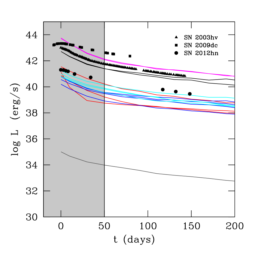
Figure 8: Bolometric late-time light curves of those dynamical interactions in which at least one of the colliding white dwarfs explodes. The colors indicate the different white dwarf pairs considered here, and is the same employed in Fig. 3: red curves stand for a $0.4\,M_{\sun}+0.4\,M_{\sun}$ system, black ones for a $0.8\,M_{\sun}+1.2\,M_{\sun}$, magenta curves denote a $0.8\,M_{\sun}+1.0\,M_{\sun}$ pair, blue ones correspond to $0.4\,M_{\sun}+0.8\,M_{\sun}$ systems, cyan lines are used for a $0.4\,M_{\sun}+1.2\,M_{\sun}$ pair, while the grey curve corresponds to the $0.2\,M_{\sun}+0.4\,M_{\sun}$ case. The light curves of three observed Type Ia supernovae are also displayed for comparison. Square symbols show the light curve of SN 2009dc, triangles correspond to SN 2003hv, while circles correspond to SN 2012hn. The gray shaded area indicates that for these early times our light curve is not entirely reliable. The time origin is set at the time at which our simulations reach the maximum temperature (explosion time). See the on-line edition of the journal for a color version of this figure.

In Fig. 8 we also display the bolometric light curves of three thermonuclear supernovae, for which late-time observations are available, to allow a meaningful comparison with the synthetic late-time light curves computed here. Squares correspond to the light curve of SN 2009dc, which was an overluminous peculiar supernova Yamanaka et al. (2009), triangles correspond to the light curve of the otherwise normal thermonuclear supernova SN 2003hv (Leloudas et al., 2009), while circles correspond to the underluminous SNIa SN 2012hn (Valenti et al., 2014). As can be seen, only a few of our simulated late-time light curves — corresponding to the brightest events — have characteristics similar to those of thermonuclear supernovae, whereas most of the dynamical interactions studied in this paper would appear as underluminous transients. In particular, only the runs in which rather massive white dwarfs interact have light curves which could be assimilated to those of SNIa. In particular, this is the case of runs number 4 and 8, in which a pair of white dwarfs with masses $0.8\,M_{\sun}$ and $1.2\,M_{\sun}$ interact — in which case only the less massive carbon-oxygen white dwarf is disrupted, while the massive ONe one remains bound — for runs 3 and 7 — which involve a pair of massive carbon-oxygen white dwarfs of masses $0.8\,M_{\sun}$ and $1.0\,M_{\sun}$, and both components are distroyed as a consequence of the interaction — and, possibly, runs number 38 and 42, which involve two white dwarfs with masses $0.4\,M_{\sun}$ and $0.4\,M_{\sun}$, and $1.2\,M_{\sun}$ and $0.4\,M_{\sun}$, respectively. Note that in these last two cases a white dwarf with a helium core is involved. Hence, the total mass burned is small, as is the mass of synthesized ⁵⁶Ni — see table 3. In summary, only those light curves resulting from events in which the total mass of the system is large (larger than $\sim 1.8\,M_{\sun}$) and a carbon-oxygen white dwarf is involved in the interaction resemble those of thermonuclear supernovae, whereas the rest of the interactions are transient bright events of different nature.

In table 3 we also show the decline rate of the bolometric light curve at late times. As well known, after about 50 days the light curves of SNIa steadily decline in an exponential way. It is observationally found that the decline rates are essentially the same for all thermonuclear supernovae between 50 and 120 days (Wells et al., 1994; Hamuy et al., 1996; Lira et al., 1998) — that is, for the time interval for which the results of our calculations are reliable — and hence, a comparison of our calculations and the observed decline rates is worthwhile. The typical values of the late-time decline rate are 0.014 mag/day in the $B$ band, 0.028 mag/day in the $V$ band, and 0.042 mag/day in the $I$ band, although there are a few exceptions (SN 1986G and SN 1991bg), which decline faster — see Leibundgut (2000), and references therein. Given our numerical approach, to compare our simulated late-time light curves with the observed decline rates of SNeIa we only used data from day 60. As shown in table 3 the computed decline rates are compatible with those observationally found in Type Ia supernovae.

3.3 Thermal neutrinos

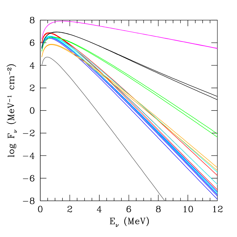
Figure 9: Spectral energy distribution of neutrinos for those interactions resulting in a direct collision. The color coding is the same employed in Fig. 3. We assumed that source of neutrinos is located at a distance of 1 kpc. See the on-line edition for a color version of this figure.

As mentioned, due to the extreme physical conditions reached in some of the interactions studied in this work it is expected that copious amounts of thermal neutrinos should be produced in those regions where the material of the colliding white dwarfs is compressed and heated. Tables 2 and 3 show that this is indeed the case. In particular, in these tables we list the energy radiated in the form of thermal neutrinos in lateral collisions and in direct ones, respectively. As can be seen, the radiated energies are in all cases rather large, although a large spread is also found. Specifically, for the case of lateral collisions the neutrino energies range from $\sim 1.7\times 10^{35}$ erg to $\sim 2.4\times 10^{45}$ erg, roughly 10 orders of magnitude, whereas in the case of direct collisions the range of variation is somewhat smaller, since it spans about 5 orders of magnitude, being run 3 the simulation in which more neutrinos are produced ($\sim 8.4\times 10^{47}$ erg). In general, we find that for the case of lateral collisions increasing the total mass of the system results in stronger interactions, and consequently larger peak temperatures and densities are achieved. This directly translates in a larger release of both nuclear energy and of thermal neutrinos — see table 2. Equally, for a fixed total mass of the system, larger mass ratios lead to a smaller nuclear energy release, and in a reduced neutrino emission. Besides, systems with larger initial distances at closest approach between both colliding white dwarfs result in longer mergers — as can be seen in column 3 of table 2, which lists the number of mass transfer episodes occurring in each lateral collision — and, therefore, in more gentle interactions, thus leading to smaller neutrino luminosities. This is in contrast with what we found for the emission of gravitational waves, for which the reverse is true. For the case of direct collisions we also find that, in general, as the total mass of the system is increased, neutrino luminosities also increase, as it happens in lateral collisions — see table 3. However, there are exceptions to this rule. Specifically, a good example of this is the case of the interactions in which two white dwarfs of masses $0.8\,M_{\sun}$ and $1.0\,M_{\sun}$ collide. In these interactions both stars are totally disrupted, and it turns out that, consequently, the nuclear energy released is larger, and that more neutrinos are produced than in the case in which a $0.8\,M_{\sun}+1.2\,M_{\sun}$ is considered. This is a consequence of the fact that in this case the more massive oxygen-neon white dwarf of $1.2\,M_{\sun}$ is more tightly gravitationally bound, and is not disrupted during the interaction.

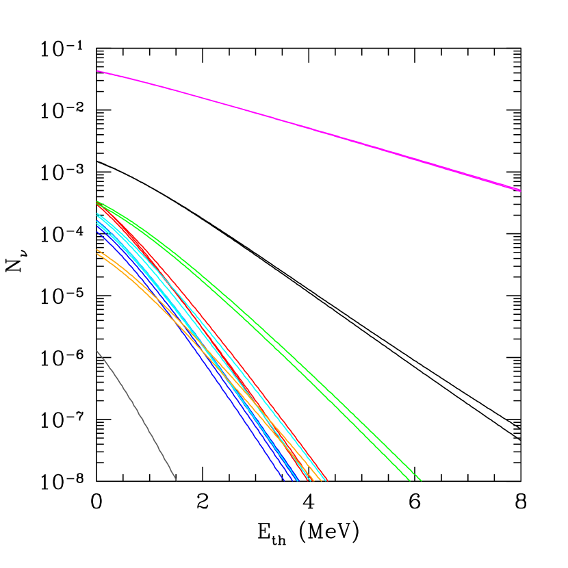
Figure 10: Expected number of neutrino events in the Super-Kamiokande detector, when the source is located at a distance of 1 kpc. Again, the color coding is the same employed in Fig. 8. See the on-line edition of the journal for a color version of this figure.

Figure 9 displays the spectral energy distribution of the neutrinos emitted when the temperature reaches its maximum value during the dynamical interaction, using the same color coding as it was done in previous figures. As expected, the general features of the neutrino spectral flux follow the same pattern previously found for the peak bolometric luminosities, and show a wide range of variation. Quite naturally, the simulations in which more ⁵⁶Ni is synthesized also produce more neutrinos. Nevertheless, this is not the most relevant information that can be obtained from this figure. Instead, it is important to note that in all cases the peak of emission corresponds to neutrinos with energies between 1 and 2 MeV. Thus, the best-suited detector for searching the neutrino signals produced in these dynamical events is the Super-Kamiokande detector (Nakahata et al., 1999), for which the peak sensitivity is 3 MeV, although other detectors, like the IceCube Observatory (Ahrens et al., 2002) could also eventually detect the neutrinos produced in these interactions (Abbasi et al., 2011). Hence, we compute the number of expected neutrino events for this detector, using the prescription outlined in Sect. 2.3. The results are shown in Fig. 10. Clearly, even for nearby sources (located at 1 kpc) only those dynamical interactions in which two very massive carbon-oxygen white dwarfs are involved will have (small) chances to be detected, since in the best of the cases only $\sim 0.04$ thermal neutrinos will interact with the tank.

3.4 Fallback luminosities

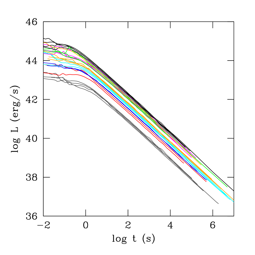
Figure 11: Fallback accretion luminosity for the dynamical interactions for which the outcome is a lateral collision, and hence result in the formation of a central remnant surrounded by a disk. The fallback accretion luminosities have been averaged over all the SPH particles with eccentric orbits for a given time. The color coding is the same of Fig. 8. See the on-line version of the journal for a color version of this figure.

Another potential observational signature of the mergers studied here is the emission of high-energy photons from the fallback material in the aftermath of those dynamical interactions in which one of the stars is disrupted, and the final configuration consists of a central remnant surrounded by a debris region. As described in depth in Aznar-Siguán et al. (2013), in some dynamical interactions a fraction of the disrupted star goes to form a Keplerian disk. In this debris region the vast majority of material has circularized orbits. However, some material in this region has highly eccentric orbits. After some time, this material will most likely interact with the recently formed disk. Rosswog (2007) demonstrated that the relevant timescale in this case is not given by viscous dissipation but, instead, by the distribution of eccentrities. As discussed in Sect. 2.4, we adopted the formulation of Rosswog (2007) and calculated the accretion luminosity resulting from the interaction of the material with high eccentricities with the newly formed disk by assuming that the kinetic energy of these particles is dissipated within the radius of the debris disk.

Figure 11 displays the results of this procedure for all the lateral collisions in which as a result of the dynamical interaction the less massive star is disrupted and a Keplerian disk is formed. We note that only a fraction of the fallback luminosity will be released in the form of high-energy photons. Thus, the results shown in this figure can be regarded as an upper limit for the actual luminosity of high-energy photons. It is important to note that the time dependence of the fallback luminosities is very similar for all the simulations, $\propto t^{-5/3}$. This time dependence is the same found for double white dwarf or double neutron star mergers. Another interesting point is that the fallback luminosities are rather high, of the order of $10^{45}$ erg s^-1, and thus these events could eventually be detected up to relatively large distances. Finally, as it should be expected, the most violent interactions result in larger fallback luminosities. In particular, the events with the largest fallback luminosities are those in which two white dwarfs with masses $0.8\,M_{\sun}$ and $1.2\,M_{\sun}$ interact (runs number 12, 16, 20 and 24, black lines), while the event in which less X-ray photons would be radiated is that in which a pair of helium white dwarfs of masses $0.2\,M_{\sun}$ and $0.4\,M_{\sun}$ collide (runs number 39, 43, 47, and 51, grey lines). Note, nevertheless, that the fallback luminosity in this case is only a factor of $10^{2}$ smaller than that computed for the most violent event. This is in contrast with the large difference (almost 9 orders of magnitude) found for the light curves of direct collisions. This, again, is a consequence of the very small amount of ⁵⁶Ni synthesized during the interaction, whereas the masses of the debris region do not differ substantially (being of the same order of magnitude). A more detailed analysis shows that the key issue to explain this behavior is that the more massive mergers produce more material in the debris region with larger kinetic energies, thus resulting in enhanced fallback luminosities.

4 Summary and conclusions

We have computed the observational signatures of the dynamical interactions of two white dwarfs in a dense stellar environment. This includes the emission of gravitational waves for those systems which as a result of the interaction end up forming an eccentric binary system, or those pairs which experience a lateral collision, in which several mass transfer episodes occur, although we also computed the emission of gravitational waves for those events in which a direct collision, in which only one violent mass transfer episode occurs. For those cases in which as a consequence of the dynamical mass transfer process an explosion occurs, and either one or both stars are disrupted, we also computed the corresponding late-time bolometric light curves, and the associated emission of thermal neutrinos, while for all those simulations in which the less massive white dwarf is disrupted, and part of its mass goes to form a debris region, we also computed the fallback luminosities radiated in the aftermath of the interaction. This has been done employing the most complete and comprehensive set of simulations of this kind — namely that of Aznar-Siguán et al. (2013) — which covers a wide range of masses, chemical compositions of the cores of the white dwarfs, and initial conditions of the intervening stars. For all these signals we have assessed the feasibility of detecting them.

We have shown that in the case of interactions leading to the formation of an eccentric binary the most noticeable feature of the emitted gravitational wave pattern is a discrete spectrum, and that these signals are likely to be detected by future spaceborne detectors, like eLISA, up to relatively long distances (larger than 10 kpc). This, however, is not the case of the gravitational wave radiation resulting from lateral collisions, although more advanced experiments, like ALIA, would be able to detect them. Finally, since for the case of direct collisions the emitted signal consists of a single, well-defined peak, of very short duration, there are no hopes to detect them.

The late-time bolometric light curves of those events in which an explosion is able to develop, and at least one of the stars is disrupted, show a broad range of variation, of almost 10 orders of magnitude in luminosity. This is the logical consequence of the large variety of masses of ⁵⁶Ni synthesized during the explosion. This, in turn, can be explained by the very different masses of the white dwarfs involved in the interaction. Even more, we have found that for a given pair of white dwarfs with fixed masses the initial conditions of the interaction — namely, the initial separations and velocities (or, alternatively, the energies and angular momenta) — also play a key role in shaping the late-time bolometric light curves, and that the corresponding peak luminosities can differ by almost 2 orders of magnitude. More interestingly, we have found that only the brightest events have light curves resembling those of thermonuclear supernovae, and that most of our simulations result in very underluminous events, which would most likely be classified as bright transient events. Only those events in which two rather massive white dwarfs (of masses larger than $\sim 0.8\,M_{\sun}$) collide would have light curves which could be assimilated to those of Type Ia supernovae. Even in this case, the resulting late-time bolometric light curves show a considerable range of variability depending on the adopted initial conditions, and light curves resembling those of underluminous, normal and peculiar bright SNIa are possible.

The corresponding thermal neutrino luminosities also show a noticeable dispersion, which is a natural consequence of the very different maximum temperatures reached during the most violent phases of the interaction. Nonetheless, the chances of detecting the neutrinos emitted in these events are very low for the current detectors, even if the dynamical interaction occurs relatively close, at 1 kpc. Even in this case, the Super-Kamiokande detector would not be able to detect the neutrino signal, since the number counts are small, $\sim 10^{-2}$ in the best of the cases.

Finally, we have also computed the emission of high-energy photons in the aftermath of those interactions in which at least one of the white dwarfs is disrupted, and a debris region is formed. As it occurs for the case of the mergers of two white dwarfs, or of two neutron stars, the accretion luminosity follows a characteristic power law of index $-5/3$, but the fallback luminosities are considerably smaller than in the case of neutron star mergers. Nevertheless, the typical peak luminosities are of the order of $10^{44}$ erg s^-1, and hence should be easily detectable up to very long distances. Again, we also find that depending on the masses and the initial conditions of the interaction the spread in the peak fallback luminosities is large, although considerably smaller than that obtained for the late-time bolometric light curves.

All in all, our calculations provide a qualitative multimessenger picture of the dynamical interactions of two white dwarfs. A combined strategy in which data obtained from the planned spaceborne gravitational wave detectors, as well as optical and high-energy observations would result in valuable insight on the conditions under which this type of events take place.

References

- Abbasi et al. (2011) Abbasi R., Abdou Y., Abu-Zayyad T., Ackermann M., Adams J., Aguilar J. A., Ahlers M., Allen M. M., Altmann D., Andeen K., et al., 2011, A&A, 535, A109
- Ahrens et al. (2002) Ahrens J., et al., 2002, Astroparticle Physics, 16, 345
- Amaro-Seoane et al. (2013) Amaro-Seoane P., et al., 2013, GW Notes, Vol. 6, p. 4-110, 6, 4
- Arnett (1979) Arnett W. D., 1979, ApJ, 230, L37
- Aznar-Siguán et al. (2013) Aznar-Siguán G., García-Berro E., Lorén-Aguilar P., José J., Isern J., 2013, MNRAS, 434, 2539
- Branch (1992) Branch D., 1992, ApJ, 392, 35
- Colgate & McKee (1969) Colgate S. A., McKee C., 1969, ApJ, 157, 623
- Crowder & Cornish (2005) Crowder J., Cornish N. J., 2005, Phys. Rev. D, 72, 083005
- Giacomazzo et al. (2011) Giacomazzo B., Rezzolla L., Baiotti L., 2011, Phys. Rev. D, 83, 044014
- Hamuy et al. (1996) Hamuy M., Phillips M. M., Suntzeff N. B., Schommer R. A., Maza J., Smith R. C., Lira P., Aviles R., 1996, AJ, 112, 2438
- Hawley et al. (2012) Hawley W. P., Athanassiadou T., Timmes F. X., 2012, ApJ, 759, 39
- Itoh et al. (1996) Itoh N., Hayashi H., Nishikawa A., Kohyama Y., 1996, ApJS, 102, 411
- Kunugise & Iwamoto (2007) Kunugise T., Iwamoto K., 2007, PASJ, 59, L57
- Kushnir et al. (2013) Kushnir D., Katz B., Dong S., Livne E., Fernández R., 2013, ApJ, 778, L37
- Leibundgut (2000) Leibundgut B., 2000, A&A Rev., 10, 179
- Leloudas et al. (2009) Leloudas G., et al., 2009, A&A, 505, 265
- Lira et al. (1998) Lira P., et al., 1998, AJ, 115, 234
- Lorén-Aguilar et al. (2005) Lorén-Aguilar P., Guerrero J., Isern J., Lobo J. A., García-Berro E., 2005, MNRAS, 356, 627
- Lorén-Aguilar et al. (2010) Lorén-Aguilar P., Isern J., García-Berro E., 2010, MNRAS, 406, 2749
- Misner et al. (1973) Misner C. W., Thorne K. S., Wheeler J. A., 1973, Gravitation. W.H. Freeman and Co.
- Nakahata et al. (1999) Nakahata M., et al., 1999, Nuclear Instruments and Methods in Physics Research A, 421, 113
- Odrzywolek & Plewa (2011) Odrzywolek A., Plewa T., 2011, A&A, 529, A156
- Pakmor et al. (2012) Pakmor R., Kromer M., Taubenberger S., Sim S. A., Röpke F. K., Hillebrandt W., 2012, ApJ, 747, L10
- Raskin et al. (2010) Raskin C., Scannapieco E., Rockefeller G., Fryer C., Diehl S., Timmes F. X., 2010, ApJ, 724, 111
- Raskin et al. (2009) Raskin C., Timmes F. X., Scannapieco E., Diehl S., Fryer C., 2009, MNRAS, 399, L156
- Rosswog (2007) Rosswog S., 2007, MNRAS, 376, L48
- Rosswog et al. (2009) Rosswog S., Kasen D., Guillochon J., Ramirez-Ruiz E., 2009, ApJ, 705, L128
- Rosswog et al. (2013) Rosswog S., Piran T., Nakar E., 2013, MNRAS, 430, 2585
- Valenti et al. (2014) Valenti S., et al., 2014, MNRAS, 437, 1519
- Wahlquist (1987) Wahlquist H., 1987, General Relativity and Gravitation, 19, 1101
- Wells et al. (1994) Wells L. A., et al., 1994, AJ, 108, 2233
- Yamanaka et al. (2009) Yamanaka M., et al., 2009, ApJ, 707, L118
- Zanotti et al. (2003) Zanotti O., Rezzolla L., Font J. A., 2003, MNRAS, 341, 832