Mind the Nuisance: Gaussian Process Classification
using Privileged Noise

Abstract

The learning with privileged information setting has recently attracted a lot of attention within the machine learning community, as it allows the integration of additional knowledge into the training process of a classifier, even when this comes in the form of a data modality that is not available at test time. Here, we show that privileged information can naturally be treated as noise in the latent function of a Gaussian Process classifier (GPC). That is, in contrast to the standard GPC setting, the latent function is not just a nuisance but a feature: it becomes a natural measure of confidence about the training data by modulating the slope of the GPC sigmoid likelihood function. Extensive experiments on public datasets show that the proposed GPC method using privileged noise, called GPC+, improves over a standard GPC without privileged knowledge, and also over the current state-of-the-art SVM-based method, SVM+. Moreover, we show that advanced neural networks and deep learning methods can be compressed as privileged information.

1 Introduction

Prior knowledge is a crucial component of any learning system, as without a form of prior knowledge, learning is provably impossible [1]. Many forms of integrating prior knowledge into machine learning algorithms have been developed: as a preference of certain prediction functions over others, as a Bayesian prior over parameters, or as additional information about the samples in the training set used for learning a prediction function. In this work, we rely on the last of these setups, adopting Vapnik and Vashist’s learning using privileged information (LUPI), see e.g. [2, 3]: we want to learn a prediction function, e.g. a classifier, and in addition to the main data modality that is to be used for prediction, the learning system has access to additional information about each training example.

This scenario has recently attracted considerable interest within the machine learning community, because it reflects well the increasingly relevant situation of learning as a service: an expert trains a machine learning system for a specific task on request from a customer. Clearly, in order to achieve the best result, the expert will use all the information available to him or her, not necessarily just the information that the system itself will have access to during its operation after deployment. Typical scenarios for learning as a service include visual inspection tasks, in which a classifier makes real-time decisions based on the input from its sensor, but at training time, additional sensors could be made use of, and the processing time per training example plays less of a role. Similarly, a classifier built into a robot or mobile device operates under strong energy constraints, while at training time, energy is less of a problem, so additional data can be generated and made use of. A third, and increasingly important scenario is when the additional data is confidential, as, e.g., in health care applications. One can expect that a diagnosis system can be improved when more information is available at training time. One might, e.g., perform specific blood test, genetic sequence, or drug trials, for the subjects that form the training set. However, the same data will not be available at test time, as obtaining it would be impractical, unethical, or outright illegal.

In this work, we propose a novel method for using privileged information based on the framework of Gaussian process classifiers (GPCs). The privileged data enters the model in form of a latent variable, which modulates the noise term of the GPC. Because the noise is integrated out before obtaining the final predictive model, the privileged information is indeed only required at training time, not at prediction time. The most interesting aspect of the proposed model is that by this procedure, the influence of the privileged information becomes very interpretable: its role is to model the confidence that the Gaussian process has about any training example, which can be directly read off from the slope of the sigmoid-shaped GPC likelihood. Training examples that are easy to classify by means of their privileged data cause a faster increasing sigmoid, which means the GP trusts the taining example and tried to fit it well. Examples that are hard to classify result in a slowly increase slope, so the GPC considers the training example less reliable and puts not a lot of effort in fitting its label well. Our experiments on multiple datasets show that this procedure leads not just to interpretable models, but also to significantly higher classification accuracy.

Related Work The LUPI framework was originally proposed by Vapnik and Vashist [2], inspired by a thought-experiment: when training a soft-margin SVM, what if an oracle would provide us with the optimal values of the slack variables? As it turns out, this would actually provably reduce the amount of training data needed, and consequently, Vapnik and Vashist proposed the SVM+ classifier that uses privileged data to predict values for the slack variables, which led to improved performance on several categorization tasks and found applications, e.g., in finance [4]. This setup was subsequently improved, by a faster training algorithm [5], better theoretical characterization [3], and it was generalized, e.g., to the learning to rank setting [6], clustering [7], and metric learning [8]. Recently, however, it was shown that the main effect of the SVM+ procedure is to assign a data-dependent weight to each training example in the SVM objective [9]. In contrast, GPC+ constitutes the first Bayesian treatment of classification using privileged information. Indeed, the resulting privileged noise approach is related to input-modulated noise commonly done in the regression task, and several Bayesian treatments of this heteroscedastic regression using Gaussian processes have been proposed. Since the predictive density and marginal likelihood are no longer analytically tractable, most works in heteroscedastic GPs deal with approximate inference; techniques such as Markov Chain Monte Carlo [10], maximum a posteriori [11], and recently a variational Bayes method [12]. To our knowledge, however, there is no prior work on heteroscedastic classification using GPs — we will elaborate the reasons in Section 2.1 — and consequently this work develops the first approximate inference based on expectation propagation for the heteroscedastic noise case in the context of classification.

2 GPC+: Gaussian Process Classification with Privileged Noise

For self-consistency of the paper, we first review the GPC model [13] with a particular emphasis on the noise-corrupted latent Gaussian process view. Then, we show how to treat privileged information as heteroscedastic noise in this latent process. The elegant aspect of this view is the intuition as how the privileged noise is able to distinguish between easy and hard samples and in turn to re-calibrate our uncertainty in the original space.

2.1 Gaussian process classifier with noisy latent process

We are given a set of $N$ input-output data points or samples $\mathcal{D}=\{(\mathbf{x}_{1},y_{1}),\ldots,(\mathbf{x}_{N},y_{N})\}\subset\mathbb{R}^{d}\times\{0,1\}$. Furthermore, we assume that the class label $y_{i}$ of sample $\mathbf{x}_{i}$ has been generated as $y_{n}=\mathbb{I}[\ \tilde{f}(\mathbf{x}_{n})\geq 0\ ]$, where $\tilde{f}(\cdot)$ is a noisy latent function and $\mathbb{I}[\cdot]$ is the Iverson’s bracket notation: $\mathbb{I}[\ P\ ]=1$ when the condition $P$ is true, and $0$ otherwise. Induced by the label generation process, we adopt the following form of likelihood function for $\mathbf{\tilde{f}}=(\tilde{f}(\mathbf{x}_{1}),\ldots,\tilde{f}(\mathbf{x}_{N}))^{\top}$:

$$\text{Pr}(\mathbf{y}|\mathbf{\tilde{f}},X=(\mathbf{x}_{1},\ldots,\mathbf{x}_{N})^{\top})=\prod\nolimits_{n=1}^{N}\text{Pr}(y_{n}=1|\mathbf{x}_{n},\tilde{f})=\prod\nolimits_{n=1}^{N}\mathbb{I}[\ \tilde{f}(\mathbf{x}_{n})\geq 0\ ],$$ (1)

where the noisy latent function at sample $\mathbf{x}_{n}$ is given by $\tilde{f}(\mathbf{x}_{n})=f(\mathbf{x}_{n})+\epsilon_{n}$ with $f(\mathbf{x}_{n})$ being the noise-free latent function. The noise term $\epsilon_{n}$ is assumed to be independent and normally distributed with zero mean and variance $\sigma^{2}$, that is $\epsilon_{n}\sim\mathcal{N}(\epsilon_{n}|0,\sigma^{2})$. To make inference about $\tilde{f}(\mathbf{x}_{n})$, we need to specify a prior over this function. We proceed by imposing a zero mean Gaussian process prior [13] on the noise-free latent function, that is $f(\mathbf{x}_{n})\sim\mathcal{GP}(0,k(\mathbf{x}_{n},\cdot))$ where $k(\cdot,\cdot)$ is a positive-definite kernel function [14] that specifies prior properties of $f(\cdot)$. A typical kernel function that allows for non-linear smooth function is the squared exponential kernel $k_{f}(\mathbf{x}_{n},\mathbf{x}_{m})=\theta\exp(-\frac{1}{2l}\left\|\mathbf{x}_{n}-\mathbf{x}_{m}\right\|^{2}_{\ell_{2}})$. In this kernel function, the parameter $\theta$ controls the amplitude of function $f(\cdot)$ while $l$ controls the smoothness of $f(\cdot)$. Given the prior and the likelihood, Bayes’ rule is used to compute the posterior of $\tilde{f}(\cdot)$, that is $\text{Pr}(\mathbf{\tilde{f}}|X,\mathbf{y})=\nicefrac{{\text{Pr}(\mathbf{y}|\mathbf{\tilde{f}},X)\text{Pr}(\mathbf{\tilde{f}})}}{{\text{Pr}(\mathbf{y}|X)}}$.

We can simplify the above noisy latent process view by integrating out the noise term $\epsilon_{n}$ and writing down the individual likelihood at sample $\mathbf{x}_{n}$ in term of noise-free latent function $f(\cdot)$ as follows

$$\text{Pr}(y_{n}=1|\mathbf{x}_{n},f) =\!\!\int\!\!\mathbb{I}[\tilde{f}(\mathbf{x}_{n})\geq 0]\mathcal{N}(\epsilon_{n}|0,\sigma^{2})d\epsilon_{n}=\!\!\int\!\!\mathbb{I}[\epsilon_{n}\geq-f(\mathbf{x}_{n})]\mathcal{N}(\epsilon_{n}|0,\sigma^{2})d\epsilon_{n}$$

$$=\Phi_{(0,\sigma^{2})}(f(\mathbf{x}_{n})),$$ (2)

where $\Phi_{(\mu,\sigma^{2})}(\cdot)$ is a Gaussian cumulative distribution function (CDF) with mean $\mu$ and variance $\sigma^{2}$. Typically the standard Gaussian CDF is used, that is $\Phi_{(0,1)}(\cdot)$, in the likelihood of (2.1). Coupled with a Gaussian process prior on the latent function $f(\cdot)$, this results in the widely adopted noise-free latent Gaussian process view with probit likelihood. The equivalence between a noise-free latent process with probit likelihood and a noisy latent process with step-function likelihood is widely known [13]. It is also widely accepted that the noisy latent function $\tilde{f}$ (or the noise-free latent function $f$) is a nuisance function as we do not observe the value of this function itself and its sole purpose is for a convenient formulation of the classification model [13]. However, in this paper, we show that by using privileged information as the noise term, the latent function $\tilde{f}$ now plays a crucial role. The latent function with privileged noise adjusts the slope transition in the Gaussian CDF to be faster or slower corresponding to more certainty or more uncertainty about the samples in the original space. This is described in details in the next section.

2.2 Privileged information is in the Nuisance Function

In the learning using privileged information (LUPI) paradigm [2], besides input data points $\{\mathbf{x}_{1},\ldots,\mathbf{x}_{N}\}$ and associated outputs $\{y_{1},\ldots,y_{N}\}$, we are given additional information $\mathbf{x}^{*}_{n}\in\mathbb{R}^{d^{*}}$ about each training instance $\mathbf{x}_{n}$. However this privileged information will not be available for unseen test instances. Our goal is to exploit the additional data $\mathbf{x}^{*}$ to influence our choice of the latent function $\tilde{f}(\cdot)$. This needs to be done while making sure that the function does not directly use the privileged data as input, as it is simply not available at test time. We achieve this naturally by treating the privileged information as a heteroscedastic (input-dependent) noise in the latent process.

Our classification model with privileged noise is then as follows:

$$\text{Likelihood model}: \ \text{Pr}(y_{n}=1|\mathbf{x}_{n},\tilde{f})=\mathbb{I}[\ \tilde{f}(\mathbf{x}_{n})\geq 0\ ]\quad\text{where}\quad\mathbf{x}_{n}\in\mathbb{R}^{d}$$ (3)

$$\text{Assume}: \ \tilde{f}(\mathbf{x}_{n})=f(\mathbf{x}_{n})+\epsilon_{n}$$ (4)

$$\text{Privileged noise model}: \ \epsilon_{n}\overset{i.i.d.}{\sim}\mathcal{N}(\epsilon_{n}|0,z(\mathbf{x}^{*}_{n})=\exp(g(\mathbf{x}^{*}_{n})))\quad\text{where}\quad\mathbf{x}^{*}_{n}\in\mathbb{R}^{d^{*}}$$ (5)

$$\text{GP prior model}: \ f(\mathbf{x}_{n})\sim\mathcal{GP}(0,k_{f}(\mathbf{x}_{n},\cdot))\quad\text{and}\quad g(\mathbf{x}^{*}_{n})\sim\mathcal{GP}(0,k_{g}(\mathbf{x}^{*}_{n},\cdot)).$$ (6)

In the above, the $\exp(\cdot)$ function is needed to ensure positivity of the noise variance. The term $k_{g}(\cdot,\cdot)$ is a positive-definite kernel function that specifies the prior properties of another latent function $g(\cdot)$ which is evaluated in the privileged space $\mathbf{x}^{*}$. Crucially, the noise term $\epsilon_{n}$ is now heteroscedastic, that is it has a different variance $z(\mathbf{x}^{*}_{n})$ at each input point $\mathbf{x}_{n}$. This is in contrast to the standard GPC approach discussed in Section 2.1 where the noise term is assumed to be homoscedastic, $\epsilon_{n}\sim\mathcal{N}(\epsilon_{n}|0,z(\mathbf{x}^{*}_{n})=\sigma^{2})$. Indeed, an input-dependent noise term is very common in a task with continuous output values $y_{n}\in\mathbb{R}$ (a regression task), resulting in the so-called heteroscedastic regression models, which have been proven to be more flexible in numerous applications as already touched upon in the related work section. However, to our knowledge, there is no prior work on heteroscedastic classification models. This is not surprising as the nuisance view of the latent function renders having a flexible input-dependent noise point-less.

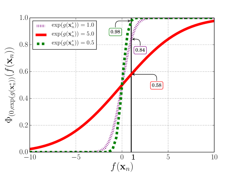
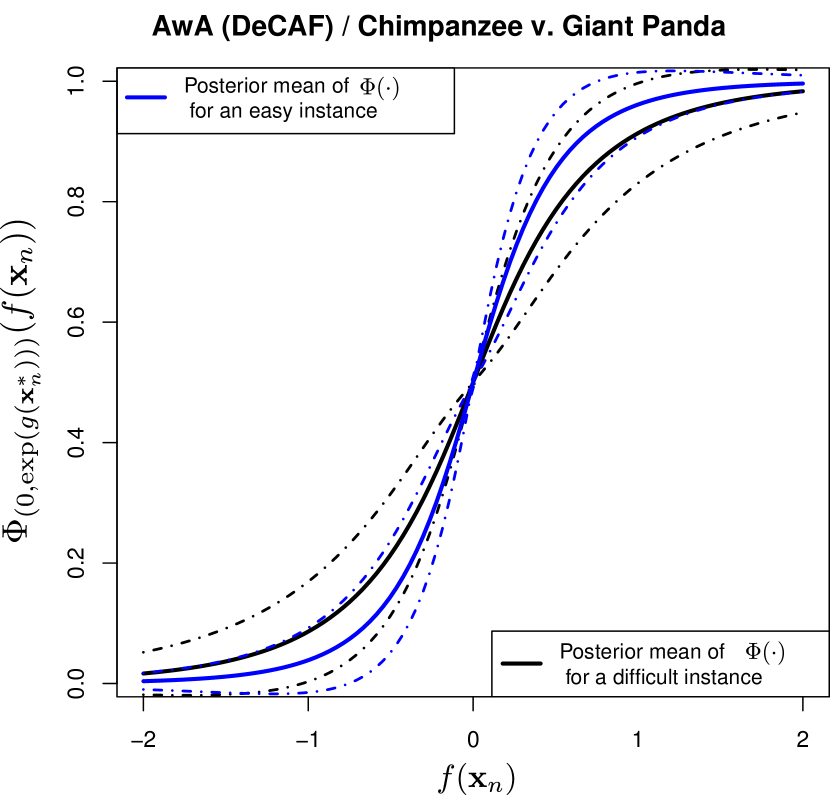
Figure 1: Effects of privileged noise on the nuisance function. (Left) On synthetic data. Suppose for an input $\mathbf{x}_{n}$, the latent function value is $f(\mathbf{x}_{n})=1$. Now also assume that the associated privileged information $\mathbf{x}_{n}^{*}$ for $n$-th data point deems the sample as difficult, say $\exp(g(\mathbf{x}^{*}_{n}))=5.0$. Then the likelihood will reflect this uncertainty $\text{Pr}(y_{n}=1|f,g,\mathbf{x}_{n},\mathbf{x}_{n}^{*})=0.58$. In contrast, if the associated privileged information considers the sample as easy, say e.g. $\exp(g(\mathbf{x}^{*}_{n}))=0.5$, the likelihood is very certain $\text{Pr}(y_{n}=1|f,g,\mathbf{x}_{n},\mathbf{x}_{n}^{*})=0.98$. (Right) On real data taken from our experiments in Sec. 4. The posterior means of the $\Phi(\cdot)$ function (solid) and its $1$-standard deviation confidence interval (dash-dot) for easy (blue) and difficult (black) instances of the Chimpanzee v. Giant Panda binary task on the Animals with Attributes (AwA) dataset. (Best viewed in color)

In the context of learning with privileged information, however, heteroscedastic classification is actually a very sensible idea. This is best illustrated when investigating the effect of privileged information in the equivalent formulation of a noise free latent process, i.e., one integrates out the privileged input-dependent noise term:

$$\text{Pr}(y_{n}=1|\mathbf{x}_{n},\mathbf{x}^{*}_{n},f,g) =\!\!\int\mathbb{I}[\ \tilde{f}(\mathbf{x}_{n})\geq 0\ ]\mathcal{N}(\epsilon_{n}|0,\exp(g(\mathbf{x}^{*}_{n}))d\epsilon_{n}$$ (7)

$$=\!\!\int\mathbb{I}[\ \epsilon_{n}\leq f(\mathbf{x}_{n})\ ]\mathcal{N}(\epsilon_{n}|0,\exp(g(\mathbf{x}^{*}_{n}))d\epsilon_{n}$$ (8)

$$=\Phi_{(0,\exp(g(\mathbf{x}^{*}_{n})))}(f(\mathbf{x}_{n}))=\Phi_{(0,1)}(f(\mathbf{x}_{n})/\sqrt{\exp(g(\mathbf{x}^{*}_{n})}).$$ (9)

From (9), it is clear that privileged information adjusts the slope transition of the Gaussian CDF. For difficult (a.k.a. noisy) samples, the latent function $g(\cdot)$ will be high, the slope transition will be slower, and thus more uncertainty is in the likelihood term $\text{Pr}(y_{n}=1|\mathbf{x}_{n},\mathbf{x}^{*}_{n},f,g)$. For easy samples, however, the latent function $g(\cdot)$ will be low, the slope transition will be faster, and thus less uncertainty is in the likelihood term $\text{Pr}(y_{n}=1|\mathbf{x}_{n},\mathbf{x}^{*}_{n},f,g)$. This is illustrated in Fig. 1.

2.3 Posterior and Prediction on Test Data

Define $\mathbf{g}=(g(\mathbf{x}_{1}^{*}),\ldots,g(\mathbf{x}_{n}^{*}))^{\text{T}}$ and $\mathbf{X}^{*}=(\mathbf{x}_{1}^{*},\ldots,\mathbf{x}_{n}^{*})^{\text{T}}$. Given the conditional i.i.d. likelihood $\text{Pr}(\mathbf{y}|\mathbf{X},\mathbf{X}^{\star},\mathbf{f},\mathbf{g})=\prod_{n=1}^{N}\text{Pr}(y_{n}=1|f,g,\mathbf{x}_{n},\mathbf{x}_{n}^{*})$ with the per observation likelihood term $\text{Pr}(y_{n}|f,g,\mathbf{x}_{n},\mathbf{x}_{n}^{*})$ given in (9) and the Gaussian process priors on functions, the posterior for $\mathbf{f}$ and $\mathbf{g}$ is:

$$\text{Pr}(\mathbf{f},\mathbf{g}|\mathbf{y},\mathbf{X},\mathbf{X}^{\star}) =\frac{\text{Pr}(\mathbf{y}|\mathbf{X},\mathbf{X}^{\star},\mathbf{f},\mathbf{g})\text{Pr}(\mathbf{f})\text{Pr}(\mathbf{g})}{\text{Pr}(\mathbf{y}|\mathbf{X},\mathbf{X}^{\star})}\,,$$ (10)

where $\text{Pr}(\mathbf{y}|\mathbf{X},\mathbf{X}^{\star})$ can be maximised with respect to a set of hyper-parameter values such as amplitude $\theta$ and smoothness $l$ parameters of the kernel functions [13]. For a previously unseen test point $\mathbf{x}_{\text{new}}\in\mathbb{R}^{d}$, the predictive distribution for its label $y_{\text{new}}$ is given as:

$$\text{Pr}(y_{\text{new}}=1|\mathbf{y},\mathbf{X},\mathbf{X}^{\star}) =\int\mathbb{I}[\ \tilde{f}(\mathbf{x}_{\text{new}})\geq 0\ ]\text{Pr}(f_{\text{new}}|\mathbf{f})\text{Pr}(\mathbf{f},\mathbf{g}|\mathbf{y},\mathbf{X},\mathbf{X}^{\star})d\mathbf{f}d\mathbf{g}df_{\text{new}}\,,$$ (11)

where $\text{Pr}(f_{\text{new}}|\mathbf{f})$ is a Gaussian conditional distribution. We note that in (11), we do not consider the privileged information $\mathbf{x}^{\star}_{\text{new}}$ associated to $\mathbf{x}_{\text{new}}$. The interpretation is we consider a homoscedastic noise at test time. This is a reasonable approach as there is no additional information for increasing or decreasing our confidence in the newly observed data $\mathbf{x}_{\text{new}}$. Finally, we predict the label for a test point via Bayesian decision theory: the label being predicted is the one with the largest probability.

3 Expectation Propagation with Numerical Quadrature

Unfortunately, as for most interesting Bayesian models, inference in the GPC+ model is very challenging. Already in the homoscedastic case, the predictive density and marginal likelihood are not analytically tractable. In this work, we therefore adapt Minka’s expectation propagation (EP) [15] with numerical quadrature for approximate inference. Please note that EP is the preferred method for approximate inference with GPCs in terms of accuracy and computational cost [16, 17].

Consider the joint distribution of $\mathbf{f}$, $\mathbf{g}$ and $\mathbf{y}$. Namely, $\text{Pr}(\mathbf{y}|\mathbf{X},\mathbf{X}^{*},\mathbf{f},\mathbf{g})\text{Pr}(\mathbf{f})\text{Pr}(\mathbf{g})$ where $\text{Pr}(\mathbf{f})$ and $\text{Pr}(\mathbf{g})$ are Gaussian process priors and the likelihood $\text{Pr}(\mathbf{y}|\mathbf{X},\mathbf{X}^{*},\mathbf{f},\mathbf{g})$ is equal to $\prod_{n=1}^{N}\text{Pr}(y_{n}|\mathbf{x}_{n},\mathbf{x}_{n}^{*},f,g)$, with $\text{Pr}(y_{n}|\mathbf{x}_{n},\mathbf{x}_{n}^{*},f,g)$ given by (9). EP approximates each non-normal factor in this joint distribution by an un-normalised bi-variate normal distribution of $f$ and $g$ (we assume independence between $f$ and $g$). The only non-normal factors correspond to those of the likelihood. These are approximated as:

$$\text{Pr}(y_{n}|\mathbf{x}_{n},\mathbf{x}_{n}^{*},f,g) \approx\overline{\gamma}_{n}(f,g)=\overline{z}_{n}\mathcal{N}(f(\mathbf{x}_{n})|\overline{m}_{f},\overline{v}_{f})\mathcal{N}(g(\mathbf{x}_{n}^{*})|\overline{m}_{g},\overline{v}_{g})\,,$$ (12)

where the parameters with the super-script $\overline{\,{}^{\,}}$ are to be found by EP. The posterior approximation $\mathcal{Q}$ computed by EP results from normalising with respect to $\mathbf{f}$ and $\mathbf{g}$ the EP approximate joint distribution. This distribution $\mathcal{Q}$ is obtained by replacing each likelihood factor by the corresponding approximate factor $\overline{\gamma}_{n}$. In particular,

$$\text{Pr}(\mathbf{f},\mathbf{g}|\mathbf{X},\mathbf{X}^{*},\mathbf{y})\approx\mathcal{Q}(\mathbf{f},\mathbf{g}):=Z^{-1}[\prod\nolimits_{n=1}^{N}\overline{\gamma}(f,g)]\text{Pr}(\mathbf{f})\text{Pr}(\mathbf{g})\,,$$ (13)

where $Z$ is a normalisation constant that approximates the model evidence $\text{Pr}(\mathbf{y}|\mathbf{X},\mathbf{X}^{*})$. The normal distribution belongs to the exponential family of probability distributions and is closed under the product and division. It is hence possible to show that $\mathcal{Q}$ is the product of two multi-variate normals [18]. The first normal approximates the posterior for $\mathbf{f}$ and the second the posterior for $\mathbf{g}$.

EP tries to fix the parameters of $\overline{\gamma}_{n}$ so that it is similar to the exact factor $\text{Pr}(y_{n}|\mathbf{x}_{n},\mathbf{x}_{n}^{*},f,g)$ in regions of high posterior probability [15]. For this, EP iteratively updates each $\overline{\gamma}_{n}$ until convergence to minimise $\text{KL}\left(\text{Pr}(y_{n}|\mathbf{x}_{n},\mathbf{x}_{n}^{\star},f,g)\mathcal{Q}^{\text{old}}/Z_{n}||\mathcal{Q}\right)$, where $\mathcal{Q}^{\text{old}}$ is a normal distribution proportional to $\left[\prod_{n^{\prime}\neq n}\overline{\gamma}_{n^{\prime}}\right]\text{Pr}(\mathbf{f})\text{Pr}(\mathbf{g})$ with all variables different from $f(\mathbf{x}_{n})$ and $g(\mathbf{x}_{n}^{*})$ marginalised out, $Z_{n}$ is simply a normalisation constant and $\text{KL}(\cdot||\cdot)$ denotes the Kullback-Leibler divergence between probability distributions. Assume $\mathcal{Q}^{\text{new}}$ is the distribution minimising the previous divergence. Then, $\overline{\gamma}_{n}\propto\mathcal{Q}^{\text{new}}/\mathcal{Q}^{\text{old}}$ and the parameter $\overline{z}_{n}$ of $\overline{\gamma}_{n}$ is fixed to guarantee that $\overline{\gamma}_{n}$ integrates the same as the exact factor with respect to $\mathcal{Q}^{\text{old}}$. The minimisation of the KL divergence involves matching expected sufficient statistics (mean and variance) between $\text{Pr}(y_{n}|\mathbf{x}_{n},\mathbf{x}_{n}^{\star},f,g)\mathcal{Q}^{\text{old}}/Z_{n}$ and $\mathcal{Q}^{\text{new}}$. These expectations can be obtained from the derivatives of $\log Z_{n}$ with respect to the (natural) parameters of $\mathcal{Q}^{\text{old}}$ [18]. Unfortunately, the computation of $\log Z_{n}$ in closed form is intractable. We show here that it can be approximated by a one dimensional quadrature. Denote by $m_{f}$, $v_{f}$, $m_{g}$ and $v_{g}$ the means and variances of $\mathcal{Q}^{\text{old}}$ for $f(\mathbf{x}_{n})$ and $g(\mathbf{x}_{n}^{*})$, respectively. Then,

$$Z_{n}=\int\Phi_{(0,1)}\left(\frac{y_{n}m_{f}}{\sqrt{v_{f}+\exp(g(\mathbf{x}_{n}^{*}))}}\right)\mathcal{N}(g(\mathbf{x}_{n}^{*})|m_{g},v_{g})dg(\mathbf{x}_{n}^{*})\,.$$ (14)

Thus, the EP algorithm only requires five quadratures to update each $\overline{\gamma}_{n}$. A first one to compute $\log Z_{n}$ and four extras to compute its derivatives with respect to $m_{f}$, $v_{f}$, $m_{g}$ and $v_{g}$. After convergence, $\mathcal{Q}$ can be used to approximate predictive distributions and the normalisation constant $Z$ can be maximised to find good values for the model’s hyper-parameters. In particular, it is possible to compute the gradient of $Z$ with respect to the parameters of the Gaussian process priors for $\mathbf{f}$ and $\mathbf{g}$ [18].

4 Experiments

Our intention here is to investigate the performance of the GP with privileged noise approach. To this aim, we considered three types of binary classification tasks corresponding to different privileged information using two real-world datasets: Attribute Discovery and Animals with Attributes. We detail those experiments in turn in the following sections.

Methods We compared our proposed GPC+ method with the well-established LUPI method based on SVM, SVM+ [5]. As a reference, we also fit standard GP and SVM classifiers when learning on the original space $\mathbb{R}^{d}$ (GPC and SVM baselines). For all four methods, we used a squared exponential kernel with amplitude parameter $\theta$ and smoothness parameter $l$. For simplicity, we set $\theta=1.0$ in all cases. For GPC and GPC+, we used type II-maximum likelihood for estimating the hyper-parameters. There are two hyper-parameters in GPC (smoothness parameter $l$ and noise variance $\sigma^{2}$) and also two in GPC+ (smoothness parameters $l$ of kernel $k_{f}(\cdot,\cdot)$ and of kernel $k_{g}(\cdot,\cdot)$). For SVM and SVM+, we used cross-validation to set the hyper-parameters. SVM has two knobs, that is smoothness and regularisation, and SVM+ has four knobs, two smoothness and two regularisation parameters. It turned out that a grid search via cross validation was too expensive for searching the best parameters in SVM+, we instead use the performance on a separate validation set to guide the search process. None of the other three methods used this separate validation set, this means that we give a competitive advantage to SVM+ over the other methods.

Evaluation metric To evaluate the performance of the methods we used classification error on an independent test set. We performed $100$ repeats of all the experiments to get the better statistics of the performance and report the mean and the standard error.

4.1 Attribute Discovery Dataset [19]

The data set was collected from a shopping website that aggregates product data from variety of e-commerce sources and includes both images and associated textual descriptions. The images and associated texts are grouped into $4$ broad shopping categories: bags, earrings, ties, and shoes. We used $1800$ samples from this dataset. We generated $6$ binary classification tasks for each pair of the $4$ classes with $200$ samples for training, $200$ samples for validation, and the rest of samples for testing the predictive performance.

Neural networks on texts as privileged information We used images as the original domain and texts as the privileged domain. This setting was also explored in [6]. However, we used a different dataset as textual descriptions of the images used in [6] are sparse and contain duplicates. Furthermore, we extracted more advanced text features instead of simple term frequency (TF) features. As image representation, we extracted SURF descriptors [20] and constructed a codebook of $100$ visual words using the $k$-means clustering. As text representation, we extracted $200$ dimensional continuous word-vector representation using a neural network skip-gram architecture [21]. To convert this word representation to a fixed-length sentence representation, we constructed a codebook of $100$ word-vector using again $k$-means clustering. We note that a more elaborate approach to transform word to sentence or document features has recently been developed [22], and we are planning to explore this in the future. We performed PCA for dimensionality reduction in the original and privileged domains and only kept the top $50$ principal components. Finally, we standardised the data so that each feature has zero mean and unit standard deviation.

The experimental results are summarised in Tab. 1. On average over $6$ tasks, SVM with hinge loss outperforms GPC with probit likelihood. However, GPC+ significantly improves over GPC providing the best results on average. This clearly shows that GPC+ is able to utilise the neural network textual representation as privileged information. In contrast, SVM+ produced the same result as SVM. We suspect this is due to: SVM has already shown strong performance on the original image space coupled with the difficulties in finding the best values of four hyper-parameters. Keep in mind that, in SVM+, we discretised the hyper-parameter search space over $625$ ($5\times 5\times 5\times 5$) possible combination values and used a separate validation technique.

	GPC		GPC+ (Ours)		SVM		SVM+
bags v. earrings	9.79$\pm$	0.12	9.50$\pm$	0.11	9.89$\pm$	0.14	9.89$\pm$	0.13
bags v. ties	10.36$\pm$	0.16	10.03$\pm$	0.15	9.44$\pm$	0.16	9.47$\pm$	0.13
bags v. shoes	9.66$\pm$	0.13	9.22$\pm$	0.11	9.31$\pm$	0.12	9.29$\pm$	0.14
earrings v. ties	10.84$\pm$	0.14	10.56$\pm$	0.13	11.15$\pm$	0.16	11.11$\pm$	0.16
earrings v. shoes	7.74$\pm$	0.11	7.33$\pm$	0.10	7.75$\pm$	0.13	7.63$\pm$	0.13
ties v. shoes	15.51$\pm$	0.16	15.54$\pm$	0.16	14.90$\pm$	0.21	15.10$\pm$	0.18
average error	10.65$\pm$	0.11	10.36$\pm$	0.12	10.41$\pm$	0.11	10.42$\pm$	0.11
average ranking	3.0		1.8		2.7		2.5

Table 1: Error rate performance (the lower the better) on the Attribute Discovery dataset over 100 repeated experiments. We used images as the original domain and neural networks word-vector representation on texts as the privileged domain. The best method for each binary task is highlighted in boldface. An average rank equal to one means that the corresponding method has the smallest error on the $6$ tasks.

DeCAF as privileged

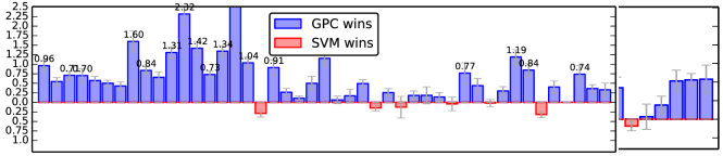
Attributes as privileged

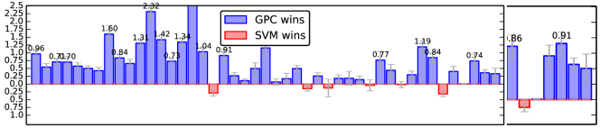
Figure 2: Pairwise comparison of the proposed GPC+ method and main baselines is shown via relative difference of the error rate (top: GPC+ versus GPC, bottom: GPC+ versus SVM+). The length of the $45$ bars corresponds to relative difference of the error rate over $45$ cases. Full results of the average error rate performance on AwA dataset across $45$ tasks over $100$ repeated experiments are in the appendix. (Best viewed in color)

4.2 Animals with Attributes (AwA) Dataset [23]

The dataset was collected by querying the image search engines for each of the $50$ animals categories which have complimentary high level description of the semantic properties such as shape, colour, or habitation forms, among others. The semantic attributes per animal class were retrieved from a prior psychological study. We focused on the $10$ categories corresponding to the test set of this dataset for which the predicted attributes are provided based on the probabilistic DAP model [23]. The $10$ classes are: chimpanzee, giant panda, leopard, persian cat, pig, hippopotamus, humpback whale, raccoon, rat, seal, and contain $6180$ images in total. As in Section 4.1 and also in [6], we generated $45$ binary classification tasks for each pair of the $10$ classes with $200$ samples for training, $200$ samples for validation, and the rest of samples for testing the predictive performance.

Neural networks on images as privileged information Deep learning methods have gained an increased attention within the machine learning and computer vision community over the recent years. This is due to their capability in extracting informative features and delivering strong predictive performance in many classification tasks. As such, we are interested to explore the use of deep learning based features as privileged information so that their predictive power can be used even if we do not have access to them at prediction time. We used the standard SURF features [20] with $2000$ visual words as the original domain and used the recently proposed DeCAF features [24] extracted from the activation of a deep convolutional network trained in a fully supervised fashion as the privileged domain. The DeCAF features were in $4096$ dimensions. All features are provided with the AwA dataset. We again performed PCA for dimensionality reduction in the original and privileged domains and only kept the top $50$ principal components, as well as standardised the data.

(DeCAF as privileged)	(Attributes as privileged)

Figure 3: Average rank (the lower the better) of the four methods and a critical distance for significant differences [25] on the AwA dataset. An average rank equal to one means that particular method has the smallest error on the $45$ tasks. Whenever the average ranks differ by more than the critical distance, there is a statistical evidence ($p$-value $<10\%$) to support a difference in the average ranks and thus in the performance. We also link two methods with a solid line if they are not statistically different from each other ($p$-value $>10\%$). In DeCAF, there is statistical evidence that GPC+ performs best among the four methods considered, while in attributes, GPC+ still performs best but there is not enough evidence to reject that GPC+ performs comparable to GPC.

Attributes as privileged information Following the experimental setting of [6], we also used images as the original domain and attributes as the privileged domain. Images were represented by $2000$ visual words based on SURF descriptors and attributes were in the form of 85 dimensional predicted attributes based on probabilistic binary classifiers [23]. This time, we only performed PCA and kept the top $50$ principal components in the original domain. Finally, we also standardised the data.

The results are summarised in Fig. 2 in term of pairwise comparison over $45$ binary tasks between GPC+ and main baselines, GPC and SVM+. The full results with the error of each method GPC, GPC+, SVM, and SVM+ on each problem are relegated to the appendix. In contrast to the results on the attribute discovery dataset, on the AwA dataset it is clear that GPC outperforms SVM in almost all of the $45$ binary classification tasks (see the appendix). The average error of GPC over $4500$ ($45$ tasks and $100$ repeats per task) experiments is much lower than SVM. On the AwA dataset, SVM+ can take advantage of privileged information – be it deep belief DeCAF features or semantic attributes – and shows significant performance improvement over SVM. However, GPC+ still shows the best overall results and further improves the already strong performance of GPC. As illustrated in Fig. 1 (right), the privileged information modulates the slope of the sigmoid likelihood function differently for easy and difficult examples: easy examples gain slope and hence importance whereas difficult ones lose importance in the classification. We analysed our experimental results using the multiple dataset statistical comparison method described in [25]. The statistical tests are summarised in Fig. 3. When DeCAF is used as privileged information, there is statistical evidence that GPC+ performs best among the four methods, while in semantic attributes as privileged information setting, GPC+ still performs best but there is not enough evidence to reject that GPC+ performs comparable to GPC.

5 Conclusions

We presented the first treatment of the learning with privileged information setting in the Gaussian process classification (GPC) framework, called GPC+. The privileged information enters the latent noise layer of the GPC+, resulting in a data-dependent modulation of the sigmoid slope of the GP likelihood. As our experimental results demonstrate this is an effective way to make use of privileged information, which manifest itself in significantly improved classification accuracies. Actually, to our knowledge, this is the first time that a heteroscedastic noise term is used to improve GPC. Furthermore, we also showed that recent advances in continuous word-vector neural networks representations [22] and deep convolutional networks for image representations [24] are privileged information. For future work, we plan to extend the GPC+ to the multiclass situation and to speed up computation by devising a quadrature-free expectation propagation method, similar to [26].

Appendix

Error rate performance on the AwA dataset over 100 repeated experiments. SURF image features as the original domain and DeCAF deep neural network image features as the privileged domain. The best methods for each binary task is highlighted in boldface.

	GPC		GPC+ (Ours)		SVM		SVM+
Chimp. v. Panda	$15.93$$\pm$	$0.15$	${\bf 15.86}$$\pm$	${\bf 0.15}$	$16.90$$\pm$	$0.15$	$16.22$$\pm$	$0.14$
Chimp. v. Leopard	$14.74$$\pm$	$0.13$	${\bf 14.69}$$\pm$	${\bf 0.12}$	$15.28$$\pm$	$0.15$	$15.10$$\pm$	$0.12$
Chimp. v. Cat	$16.63$$\pm$	$0.12$	${\bf 16.52}$$\pm$	${\bf 0.11}$	$17.34$$\pm$	$0.11$	$16.97$$\pm$	$0.11$
Chimp. v. Pig	$19.82$$\pm$	$0.23$	${\bf 19.48}$$\pm$	${\bf 0.26}$	$20.52$$\pm$	$0.27$	$20.04$$\pm$	$0.25$
Chimp. v. Hippo.	$18.99$$\pm$	$0.11$	${\bf 18.67}$$\pm$	${\bf 0.11}$	$19.57$$\pm$	$0.11$	$19.20$$\pm$	$0.11$
Chimp. v. Whale	${\bf 5.72}$$\pm$	${\bf 0.08}$	$5.79$$\pm$	$0.08$	$6.22$$\pm$	$0.11$	$5.85$$\pm$	$0.10$
Chimp. v. Raccoon	${\bf 19.60}$$\pm$	${\bf 0.13}$	$19.65$$\pm$	$0.13$	$20.03$$\pm$	$0.14$	$19.86$$\pm$	$0.13$
Chimp. v. Rat	$19.94$$\pm$	$0.27$	${\bf 19.79}$$\pm$	${\bf 0.26}$	$21.53$$\pm$	$0.30$	$20.45$$\pm$	$0.27$
Chimp. v. Seal	$14.10$$\pm$	$0.12$	${\bf 14.01}$$\pm$	${\bf 0.12}$	$14.94$$\pm$	$0.12$	$14.34$$\pm$	$0.13$
Panda v. Leopard	${\bf 14.19}$$\pm$	${\bf 0.12}$	$14.26$$\pm$	$0.13$	$14.85$$\pm$	$0.15$	$14.59$$\pm$	$0.15$
Panda v. Cat	${\bf 12.96}$$\pm$	${\bf 0.12}$	$12.99$$\pm$	$0.12$	$14.26$$\pm$	$0.13$	$13.52$$\pm$	$0.13$
Panda v. Pig	$20.23$$\pm$	$0.23$	${\bf 20.17}$$\pm$	${\bf 0.22}$	$22.54$$\pm$	$0.29$	$20.85$$\pm$	$0.24$
Panda v. Hippo.	$15.47$$\pm$	$0.12$	${\bf 15.45}$$\pm$	${\bf 0.13}$	$16.89$$\pm$	$0.17$	$15.70$$\pm$	$0.14$
Panda v. Whale	$5.00$$\pm$	$0.09$	$5.20$$\pm$	$0.09$	$5.73$$\pm$	$0.11$	${\bf 4.95}$$\pm$	${\bf 0.09}$
Panda v. Raccoon	${\bf 17.03}$$\pm$	${\bf 0.13}$	$17.04$$\pm$	$0.13$	$18.37$$\pm$	$0.18$	$17.54$$\pm$	$0.14$
Panda v. Rat	${\bf 17.09}$$\pm$	${\bf 0.24}$	$17.27$$\pm$	$0.23$	$20.06$$\pm$	$0.30$	$18.04$$\pm$	$0.25$
Panda v. Seal	$14.13$$\pm$	$0.13$	${\bf 14.01}$$\pm$	${\bf 0.12}$	$15.16$$\pm$	$0.17$	$14.22$$\pm$	$0.13$
Leopard v. Cat	$12.08$$\pm$	$0.11$	${\bf 11.77}$$\pm$	${\bf 0.09}$	$11.79$$\pm$	$0.08$	$11.82$$\pm$	$0.09$
Leopard v. Pig	${\bf 20.97}$$\pm$	${\bf 0.24}$	$21.12$$\pm$	$0.24$	$21.88$$\pm$	$0.24$	$21.79$$\pm$	$0.26$
Leopard v. Hippo.	$16.10$$\pm$	$0.14$	${\bf 15.89}$$\pm$	${\bf 0.13}$	$16.36$$\pm$	$0.13$	$16.27$$\pm$	$0.14$
Leopard v. Whale	$4.85$$\pm$	$0.07$	${\bf 4.79}$$\pm$	${\bf 0.07}$	$4.95$$\pm$	$0.08$	$4.89$$\pm$	$0.07$
Leopard v. Raccoon	$26.43$$\pm$	$0.17$	${\bf 26.24}$$\pm$	${\bf 0.16}$	$26.93$$\pm$	$0.20$	$26.74$$\pm$	$0.19$
Leopard v. Rat	${\bf 17.62}$$\pm$	${\bf 0.20}$	$17.75$$\pm$	$0.21$	$18.78$$\pm$	$0.25$	$18.00$$\pm$	$0.23$
Leopard v. Seal	$13.26$$\pm$	$0.10$	${\bf 13.05}$$\pm$	${\bf 0.10}$	$13.33$$\pm$	$0.10$	$13.35$$\pm$	$0.10$
Cat v. Pig	$24.35$$\pm$	$0.24$	${\bf 23.95}$$\pm$	${\bf 0.22}$	$24.52$$\pm$	$0.24$	$24.53$$\pm$	$0.25$
Cat v. Hippo.	$15.02$$\pm$	$0.10$	${\bf 14.85}$$\pm$	${\bf 0.10}$	$15.52$$\pm$	$0.12$	$15.26$$\pm$	$0.11$
Cat v. Whale	$7.66$$\pm$	$0.09$	$7.63$$\pm$	$0.09$	$7.51$$\pm$	$0.09$	${\bf 7.41}$$\pm$	${\bf 0.10}$
Cat v. Raccoon	$15.54$$\pm$	$0.11$	${\bf 15.35}$$\pm$	${\bf 0.10}$	$15.80$$\pm$	$0.10$	$15.71$$\pm$	$0.13$
Cat v. Rat	$34.96$$\pm$	$0.30$	$34.30$$\pm$	$0.30$	$34.83$$\pm$	$0.32$	${\bf 34.07}$$\pm$	${\bf 0.32}$
Cat v. Seal	$18.79$$\pm$	$0.14$	${\bf 18.58}$$\pm$	${\bf 0.13}$	$18.97$$\pm$	$0.14$	$18.85$$\pm$	$0.13$
Pig v. Hippo.	$27.57$$\pm$	$0.27$	${\bf 27.27}$$\pm$	${\bf 0.27}$	$27.75$$\pm$	$0.25$	$27.72$$\pm$	$0.27$
Pig v. Whale	$8.37$$\pm$	$0.15$	${\bf 8.22}$$\pm$	${\bf 0.16}$	$8.51$$\pm$	$0.17$	$8.24$$\pm$	$0.16$
Pig v. Raccoon	$24.45$$\pm$	$0.24$	${\bf 24.23}$$\pm$	${\bf 0.23}$	$24.40$$\pm$	$0.25$	$24.34$$\pm$	$0.25$
Pig v. Rat	$30.00$$\pm$	$0.26$	${\bf 29.62}$$\pm$	${\bf 0.26}$	$30.77$$\pm$	$0.30$	$30.22$$\pm$	$0.28$
Pig v. Seal	$23.91$$\pm$	$0.24$	${\bf 23.37}$$\pm$	${\bf 0.21}$	$24.35$$\pm$	$0.23$	$23.79$$\pm$	$0.22$
Hippo. v. Whale	$14.03$$\pm$	$0.12$	${\bf 13.80}$$\pm$	${\bf 0.12}$	$14.01$$\pm$	$0.12$	$14.01$$\pm$	$0.10$
Hippo. v. Raccoon	$19.31$$\pm$	$0.14$	${\bf 19.14}$$\pm$	${\bf 0.13}$	$19.61$$\pm$	$0.15$	$19.52$$\pm$	$0.13$
Hippo. v. Rat	${\bf 21.49}$$\pm$	${\bf 0.27}$	$21.82$$\pm$	$0.26$	$22.67$$\pm$	$0.26$	$22.44$$\pm$	$0.27$
Hippo. v. Seal	$30.68$$\pm$	$0.17$	${\bf 30.60}$$\pm$	${\bf 0.18}$	$31.52$$\pm$	$0.18$	$31.03$$\pm$	$0.19$
Whale v. Raccoon	$7.92$$\pm$	$0.09$	$7.77$$\pm$	$0.08$	${\bf 7.61}$$\pm$	${\bf 0.09}$	$7.68$$\pm$	$0.09$
Whale v. Rat	${\bf 10.98}$$\pm$	${\bf 0.22}$	$11.14$$\pm$	$0.22$	$11.38$$\pm$	$0.24$	$11.17$$\pm$	$0.24$
Whale v. Seal	$18.57$$\pm$	$0.16$	${\bf 18.18}$$\pm$	${\bf 0.16}$	$18.58$$\pm$	$0.18$	$18.37$$\pm$	$0.16$
Raccoon v. Rat	${\bf 25.16}$$\pm$	${\bf 0.27}$	$25.22$$\pm$	$0.25$	$25.90$$\pm$	$0.24$	$25.73$$\pm$	$0.25$
Raccoon v. Seal	$15.06$$\pm$	$0.13$	${\bf 14.82}$$\pm$	${\bf 0.13}$	$15.43$$\pm$	$0.12$	$15.35$$\pm$	$0.12$
Rat v. Seal	$24.91$$\pm$	$0.28$	${\bf 24.63}$$\pm$	${\bf 0.27}$	$25.24$$\pm$	$0.28$	$25.16$$\pm$	$0.28$
average ranking	2.09		1.40		3.71		2.80
average error	17.60$\pm$	0.10	17.47$\pm$	0.10	18.21$\pm$	0.11	17.80$\pm$	0.10

Error rate performance on the AwA dataset over 100 repeated experiments. SURF image features as the original domain and attributes as the privileged domain. The best methods for each binary task is highlighted in boldface

	GPC		GPC+ (Ours)		SVM		SVM+
Chimp. v. Panda	$15.93$$\pm$	$0.15$	${\bf 15.85}$$\pm$	${\bf 0.14}$	$16.90$$\pm$	$0.15$	$16.64$$\pm$	$0.15$
Chimp. v. Leopard	$14.74$$\pm$	$0.13$	${\bf 14.72}$$\pm$	${\bf 0.12}$	$15.28$$\pm$	$0.15$	$15.18$$\pm$	$0.12$
Chimp. v. Cat	$16.63$$\pm$	$0.12$	${\bf 16.51}$$\pm$	${\bf 0.11}$	$17.34$$\pm$	$0.11$	$17.08$$\pm$	$0.10$
Chimp. v. Pig	$19.82$$\pm$	$0.23$	${\bf 19.50}$$\pm$	${\bf 0.26}$	$20.52$$\pm$	$0.27$	$20.34$$\pm$	$0.24$
Chimp. v. Hippo.	$18.99$$\pm$	$0.11$	${\bf 18.68}$$\pm$	${\bf 0.11}$	$19.57$$\pm$	$0.11$	$19.36$$\pm$	$0.11$
Chimp. v. Whale	$5.72$$\pm$	$0.08$	$5.79$$\pm$	$0.08$	$6.22$$\pm$	$0.11$	${\bf 5.63}$$\pm$	${\bf 0.08}$
Chimp. v. Raccoon	${\bf 19.60}$$\pm$	${\bf 0.13}$	$19.66$$\pm$	$0.13$	$20.03$$\pm$	$0.14$	$20.13$$\pm$	$0.13$
Chimp. v. Rat	$19.94$$\pm$	$0.27$	${\bf 19.82}$$\pm$	${\bf 0.26}$	$21.53$$\pm$	$0.30$	$20.22$$\pm$	$0.28$
Chimp. v. Seal	$14.10$$\pm$	$0.12$	${\bf 14.03}$$\pm$	${\bf 0.12}$	$14.94$$\pm$	$0.12$	$14.57$$\pm$	$0.15$
Panda v. Leopard	${\bf 14.19}$$\pm$	${\bf 0.12}$	$14.21$$\pm$	$0.13$	$14.85$$\pm$	$0.15$	$14.82$$\pm$	$0.14$
Panda v. Cat	${\bf 12.96}$$\pm$	${\bf 0.12}$	$12.98$$\pm$	$0.12$	$14.26$$\pm$	$0.13$	$13.96$$\pm$	$0.12$
Panda v. Pig	$20.23$$\pm$	$0.23$	${\bf 20.18}$$\pm$	${\bf 0.22}$	$22.54$$\pm$	$0.29$	$21.41$$\pm$	$0.26$
Panda v. Hippo.	$15.47$$\pm$	$0.12$	${\bf 15.44}$$\pm$	${\bf 0.13}$	$16.89$$\pm$	$0.17$	$16.16$$\pm$	$0.17$
Panda v. Whale	${\bf 5.00}$$\pm$	${\bf 0.09}$	$5.20$$\pm$	$0.09$	$5.73$$\pm$	$0.11$	$5.06$$\pm$	$0.08$
Panda v. Raccoon	$17.03$$\pm$	$0.13$	${\bf 17.02}$$\pm$	${\bf 0.13}$	$18.37$$\pm$	$0.18$	$18.06$$\pm$	$0.15$
Panda v. Rat	${\bf 17.09}$$\pm$	${\bf 0.24}$	$17.26$$\pm$	$0.23$	$20.06$$\pm$	$0.30$	$18.37$$\pm$	$0.25$
Panda v. Seal	$14.13$$\pm$	$0.13$	${\bf 13.99}$$\pm$	${\bf 0.13}$	$15.16$$\pm$	$0.17$	$14.82$$\pm$	$0.15$
Leopard v. Cat	$12.08$$\pm$	$0.11$	$11.81$$\pm$	$0.09$	${\bf 11.79}$$\pm$	${\bf 0.08}$	$12.13$$\pm$	$0.11$
Leopard v. Pig	${\bf 20.97}$$\pm$	${\bf 0.24}$	$21.11$$\pm$	$0.24$	$21.88$$\pm$	$0.24$	$22.03$$\pm$	$0.29$
Leopard v. Hippo.	$16.10$$\pm$	$0.14$	${\bf 15.87}$$\pm$	${\bf 0.13}$	$16.36$$\pm$	$0.13$	$16.41$$\pm$	$0.14$
Leopard v. Whale	$4.85$$\pm$	$0.07$	${\bf 4.78}$$\pm$	${\bf 0.07}$	$4.95$$\pm$	$0.08$	$4.90$$\pm$	$0.07$
Leopard v. Raccoon	$26.43$$\pm$	$0.17$	${\bf 26.27}$$\pm$	${\bf 0.17}$	$26.93$$\pm$	$0.20$	$27.31$$\pm$	$0.19$
Leopard v. Rat	${\bf 17.62}$$\pm$	${\bf 0.20}$	$17.67$$\pm$	$0.21$	$18.78$$\pm$	$0.25$	$18.84$$\pm$	$0.24$
Leopard v. Seal	$13.26$$\pm$	$0.10$	${\bf 13.04}$$\pm$	${\bf 0.10}$	$13.33$$\pm$	$0.10$	$13.38$$\pm$	$0.10$
Cat v. Pig	$24.35$$\pm$	$0.24$	${\bf 24.01}$$\pm$	${\bf 0.23}$	$24.52$$\pm$	$0.24$	$24.68$$\pm$	$0.25$
Cat v. Hippo.	$15.02$$\pm$	$0.10$	${\bf 14.87}$$\pm$	${\bf 0.10}$	$15.52$$\pm$	$0.12$	$15.47$$\pm$	$0.11$
Cat v. Whale	$7.66$$\pm$	$0.09$	$7.63$$\pm$	$0.09$	$7.51$$\pm$	$0.09$	${\bf 7.48}$$\pm$	${\bf 0.09}$
Cat v. Raccoon	$15.54$$\pm$	$0.11$	${\bf 15.32}$$\pm$	${\bf 0.10}$	$15.80$$\pm$	$0.10$	$15.78$$\pm$	$0.10$
Cat v. Rat	$34.96$$\pm$	$0.30$	${\bf 34.42}$$\pm$	${\bf 0.29}$	$34.83$$\pm$	$0.32$	$34.79$$\pm$	$0.28$
Cat v. Seal	$18.79$$\pm$	$0.14$	${\bf 18.60}$$\pm$	${\bf 0.13}$	$18.97$$\pm$	$0.14$	$19.25$$\pm$	$0.16$
Pig v. Hippo.	$27.57$$\pm$	$0.27$	${\bf 27.36}$$\pm$	${\bf 0.26}$	$27.75$$\pm$	$0.25$	$28.17$$\pm$	$0.26$
Pig v. Whale	$8.37$$\pm$	$0.15$	${\bf 8.24}$$\pm$	${\bf 0.16}$	$8.51$$\pm$	$0.17$	$8.38$$\pm$	$0.15$
Pig v. Raccoon	$24.45$$\pm$	$0.24$	${\bf 24.24}$$\pm$	${\bf 0.22}$	$24.40$$\pm$	$0.25$	$24.91$$\pm$	$0.22$
Pig v. Rat	$30.00$$\pm$	$0.26$	${\bf 29.67}$$\pm$	${\bf 0.26}$	$30.77$$\pm$	$0.30$	$30.33$$\pm$	$0.29$
Pig v. Seal	$23.91$$\pm$	$0.24$	${\bf 23.41}$$\pm$	${\bf 0.22}$	$24.35$$\pm$	$0.23$	$24.03$$\pm$	$0.23$
Hippo. v. Whale	$14.03$$\pm$	$0.12$	${\bf 13.82}$$\pm$	${\bf 0.12}$	$14.01$$\pm$	$0.12$	$14.45$$\pm$	$0.13$
Hippo. v. Raccoon	$19.31$$\pm$	$0.14$	${\bf 19.15}$$\pm$	${\bf 0.13}$	$19.61$$\pm$	$0.15$	$19.74$$\pm$	$0.16$
Hippo. v. Rat	${\bf 21.49}$$\pm$	${\bf 0.27}$	$21.79$$\pm$	$0.26$	$22.67$$\pm$	$0.26$	$22.33$$\pm$	$0.26$
Hippo. v. Seal	$30.68$$\pm$	$0.17$	${\bf 30.61}$$\pm$	${\bf 0.18}$	$31.52$$\pm$	$0.18$	$31.47$$\pm$	$0.19$
Whale v. Raccoon	$7.92$$\pm$	$0.09$	$7.79$$\pm$	$0.08$	${\bf 7.61}$$\pm$	${\bf 0.09}$	$7.66$$\pm$	$0.08$
Whale v. Rat	${\bf 10.98}$$\pm$	${\bf 0.22}$	$11.16$$\pm$	$0.22$	$11.38$$\pm$	$0.24$	$11.17$$\pm$	$0.22$
Whale v. Seal	$18.57$$\pm$	$0.16$	${\bf 18.28}$$\pm$	${\bf 0.16}$	$18.58$$\pm$	$0.18$	$18.99$$\pm$	$0.18$
Raccoon v. Rat	${\bf 25.16}$$\pm$	${\bf 0.27}$	$25.21$$\pm$	$0.25$	$25.90$$\pm$	$0.24$	$26.12$$\pm$	$0.26$
Raccoon v. Seal	$15.06$$\pm$	$0.13$	${\bf 14.85}$$\pm$	${\bf 0.12}$	$15.43$$\pm$	$0.12$	$15.42$$\pm$	$0.13$
Rat v. Seal	$24.91$$\pm$	$0.28$	${\bf 24.64}$$\pm$	${\bf 0.26}$	$25.24$$\pm$	$0.28$	$25.14$$\pm$	$0.27$
average ranking	1.98		1.40		3.44		3.18
average error	17.60$\pm$	0.10	17.48$\pm$	0.10	18.21$\pm$	0.11	18.06$\pm$	0.11

References

- [1] D.H. Wolpert. The lack of a priori distinctions between learning algorithms. Neural computation, 8(7):1341–1390, 1996.
- [2] V. Vapnik and A. Vashist. A new learning paradigm: Learning using privileged information. Neural Networks, 22(5–6):544 – 557, 2009.
- [3] D. Pechyony and V. Vapnik. On the theory of learning with privileged information. In Advances in Neural Information Processing Systems (NIPS), 2010.
- [4] B. Ribeiro, C. Silva, A. Vieira, A. Gaspar-Cunha, and J.C. das Neves. Financial distress model prediction using SVM+. In International Joint Conference on Neural Networks (IJCNN), 2010.
- [5] D. Pechyony and V. Vapnik. Fast optimization algorithms for solving SVM+. In Statistical Learning and Data Science, 2011.
- [6] V. Sharmanska, N. Quadrianto, and C. H. Lampert. Learning to rank using privileged information. In International Conference on Computer Vision (ICCV), 2013.
- [7] J. Feyereisl and U. Aickelin. Privileged information for data clustering. Information Sciences, 194:4–23, 2012.
- [8] S. Fouad, P. Tino, S. Raychaudhury, and P. Schneider. Incorporating privileged information through metric learning. IEEE Transactions on Neural Networks and Learning Systems, 2013.
- [9] M. Lapin, M. Hein, and B. Schiele. Learning using privileged information: SVM+ and weighted SVM. Neural Networks, 53:95–108, 2014.
- [10] P. W. Goldberg, C. K. I. Williams, and C. M. Bishop. Regression with input-dependent noise: A gaussian process treatment. In Advances in Neural Information Processing Systems (NIPS), 1998.
- [11] N. Quadrianto, K. Kersting, M. D. Reid, T. S. Caetano, and W. L. Buntine. Kernel conditional quantile estimation via reduction revisited. In International Conference on Data Mining (ICDM), 2009.
- [12] M. Lázaro-Gredilla and M. K. Titsias. Variational heteroscedastic gaussian process regression. In International Conference on Machine Learning (ICML), 2011.
- [13] C. E. Rasmussen and C. K. I. Williams. Gaussian Processes for Machine Learning (Adaptive Computation and Machine Learning). The MIT Press, 2006.
- [14] B. Scholkopf and A. J. Smola. Learning with Kernels: Support Vector Machines, Regularization, Optimization, and Beyond. MIT Press, Cambridge, MA, USA, 2001.
- [15] T. P. Minka. A Family of Algorithms for Approximate Bayesian Inference. PhD thesis, Massachusetts Institute of Technology, 2001.
- [16] H. Nickisch and C. E. Rasmussen. Approximations for Binary Gaussian Process Classification. Journal of Machine Learning Research, 9:2035–2078, 2008.
- [17] M. Kuss and C. E. Rasmussen. Assessing approximate inference for binary Gaussian process classification. Journal of Machine Learning Research, 6:1679–1704, 2005.
- [18] M. Seeger. Expectation propagation for exponential families. Technical report, Department of EECS, University of California, Berkeley, 2006.
- [19] T. L. Berg, A. C. Berg, and J. Shih. Automatic attribute discovery and characterization from noisy web data. In European Conference on Computer Vision (ECCV), 2010.
- [20] H. Bay, A. Ess, T. Tuytelaars, and L. Van Gool. Speeded-up robust features (surf). Computer Vision and Image Understanding, 110(3):346–359, June 2008.
- [21] T. Mikolov, I. Sutskever, K. Chen, G. Corrado, and J. Dean. Distributed representations of words and phrases and their compositionality. In Advances in Neural Information Processing Systems (NIPS), 2013.
- [22] Q. V. Le and T. Mikolov. Distributed representations of sentences and documents. In International Conference on Machine Learning (ICML), 2014.
- [23] C. H. Lampert, H. Nickisch, and S. Harmeling. Attribute-based classification for zero-shot visual object categorization. IEEE Transactions on Pattern Analysis and Machine Intelligence, 36(3):453–465, 2014.
- [24] J. Donahue, Y. Jia, O. Vinyals, J. Hoffman, N. Zhang, E. Tzeng, and T. Darrell. Decaf: A deep convolutional activation feature for generic visual recognition. In International Conference on Machine Learning (ICML), 2014.
- [25] J. Demšar. Statistical comparisons of classifiers over multiple data sets. Journal of Machine Learning Research, 7:1–30, 2006.
- [26] J. Riihimäki, P. Jylänki, and A. Vehtari. Nested Expectation Propagation for Gaussian Process Classification with a Multinomial Probit Likelihood. Journal of Machine Learning Research, 14:75–109, 2013.