Breakup of three particles within the adiabatic expansion method.

Abstract

General expressions for the breakup cross sections in the lab frame for $1+2$ reactions are given in terms of the hyperspherical adiabatic basis. The three-body wave function is expanded in this basis and the corresponding hyperradial functions are obtained by solving a set of second order differential equations. The ${\cal S}$-matrix is computed by using two recently derived integral relations. Even though the method is shown to be well suited to describe $1+2$ processes, there are nevertheless particular configurations in the breakup channel (for example those in which two particles move away close to each other in a relative zero-energy state) that need a huge number of basis states. This pathology manifests itself in the extremely slow convergence of the breakup amplitude in terms of the hyperspherical harmonic basis used to construct the adiabatic channels. To overcome this difficulty the breakup amplitude is extracted from an integral relation as well. For the sake of illustration, we consider neutron-deuteron scattering. The results are compared to the available benchmark calculations.

I Introduction

The use of the hyperspherical adiabatic (HA) expansion method nie01 to describe a $1+2$ collision between a particle and a bound state of two particles, called dimer in atomic physics or the deuteron in nuclear physics, was considered to be rather inefficient due to the slow pattern of convergence of the elastic channel bar09 . This fact seemed to limit the applicability of the method only to the description of bound states. The problem is due to the fact that the hyperradial coordinate used in the adiabatic expansion is not suitable to describe the asymptotic behavior of the elastic outgoing wave. In this case the use of the relative coordinate between the two particles in the outgoing dimer, and the one between the center of mass of the dimer and the third particle is much more convenient. In particular, due to the finite size of the dimer, this last relative coordinate and the hyperradius coincide only at infinity. For this reason, a correct description of the asymptotic 1+2 wave function and, therefore the determination of the ${\cal S}$-matrix, requires knowledge of the wave function at very large distances, which in turn requires a huge amount of terms in the adiabatic expansion bar09b .

A new method, based on two integral relations derived from the Kohn variational principle (KVP), was introduced in bar09b in order to permit the determination of the elastic ${\cal S}$-matrix from the internal part of the wave function. Therefore, when used together with the adiabatic expansion method, the number of adiabatic terms needed in the calculation is much lower. In fact, the pattern of convergence is similar to that observed for bound states bar09b . The details of the procedure for elastic, inelastic and recombination processes are given in Refs.rom11 ; kie10 for energies below the dimer breakup threshold. The extension to treat the elastic channel at energies above the breakup threshold was discussed in Ref.gar12 .

The knowledge of the elastic, inelastic and recombination ${\cal S}$-matrix elements can be used to compute different observables characterizing the reaction. Furthermore, using the unitary condition

$$\sum_{m}^{M}|S_{im}|^{2}+\sum_{n}^{\infty}|{\cal S}_{in}|^{2}=1\,\,,$$ (1)

where $m$ indicates the finite set $M$ of the elastic, inelastic and recombination channels and $n$ labels the infinite set of breakup channels, it is possible to obtain the total breakup cross section

$$\sigma_{b}=\frac{\pi}{k^{2}}(1-\sum_{m}^{M}|S_{im}|^{2})$$ (2)

where, for three particles with equal mass, we have that $k^{2}=(4/3)E_{i}(\hbar^{2}/m)$ and $E_{i}$ is the incident energy in the center of mass frame. Examples of this procedure can be found in Refs.gar12 ; gar13 where the inelasticities in $n-d$ scattering have been computed as well as the recombination and dissociation rates in the direct and inverse atomic processes ${}^{4}{\rm He}+{}^{4}{\rm He}+{}^{4}{\rm He}\rightarrow{}^{4}{\rm He}_{2}+{}^{4}{\rm He}$. Therefore, an accurate calculation of the elastic and, if allowed, inelastic and recombination ${\cal S}$-matrix elements leads to an accurate determination of the corresponding total breakup cross section through the unitary condition.

On the other hand, when the knowledge of the breakup amplitude is required, the $S_{in}$ matrix elements have to be computed explicitly. Using the HA method, the index $n$ is related to the number of adiabatic channels taken into account in the description of the three-body scattering wave function. In the present work each adiabatic channel is expanded in the hyperspherical harmonic basis (HH). Therefore a study of the convergence properties of the breakup amplitude in terms of the adiabatic channels and the HH basis is in order. These two convergencies have to be achieved separately. As we will see, the number of adiabatic channels needed to describe the elastic channel with high accuracy is sufficient for an accurate determination of the breakup amplitude. However there are particular kinematic conditions of the outgoing particles in which the convergence of the breakup amplitude is terms of the HH basis becomes very delicate. This is the case when two of the particles move away close to each other with almost zero relative energy. In order to treat this specific configuration we will make use of an integral relation for the breakup amplitude as discussed for example in Ref. payne00 .

The method discussed in the present work is general and can be applied to different kinds of three-body reactions. In this work we shall consider the $N-d$ case, which is frequently described using the Faddeev equations, as shown for instance in Refs.wgreport ; screport or in the recent review of Ref.car14 , or using the HH formalism in conjunction with the KVP kiev01 . Calculation using the Faddeev equations in momentum space including the Coulomb force between the two protons can be found in Ref. deltuva05 . This and the HH method have been compared in the elastic channel up to $65$ MeV dfk05 . Attempts to explicitly determine the breakup amplitude using the HH formalism can be found in Refs. kiev97 ; kiev99 whereas the formalism using the KVP is discussed in Ref. viv01 . Those calculations have shown the intrinsic difficulties of a variational description of the breakup amplitude. As mentioned above, the main problem appears in the description of particular kinematics as for example the case in which two particles, for instance two neutrons travel close to each in a relative zero-energy state. This configuration represents a kind of clusterization inside the breakup amplitude and requires a huge number of basis states to be described properly.

Using the experience gained in Refs rom11 ; kie10 ; gar12 in which the HA method was used to describe elastic, inelastic and recombination processes by means of two integral relations derived from the KVP, in the present work we extend the HA method to describe the breakup amplitude explicitly. Expressions for the differential cross sections in the lab frame for $1+2$ reactions at incident energies above the dimer breakup threshold are derived. The neutron-deuteron ($n-d$) reaction is studied with a semi-realistic $s$-wave force for illustration. This choice is motivated by the existence of benchmark calculations fri95 which allow a test of the method. This study is a first step in the application of the method to describe $N-d$ scattering using realistic two- and three-body forces and including the Coulomb interaction.

In the first part of the paper we provide the details of the formalism used to compute the differential cross sections. This part is divided into several subsections where we give the expression of the cross section in the lab frame, the expansion of the transition amplitude in terms of HA functions and, finally, an integral relation to compute the transition amplitude which removes the convergence problem inherent to the HA expansion. In Section III the computation of the integral relation is discussed, in particular the treatment of the long tail of the kernel. The results obtained for the case of neutron-deuteron breakup are described in Section IV and the last section is devoted to some conclusive remarks. For the sake of completeness, the paper includes six appendices in which some derivations not essential for the understanding of the paper are given. In particular, several technical aspects of the scattering theory are discussed in terms of the hyperspherical adiabatic expansion method.

II Formalism

In this section we summarize the formalism employed to compute the differential cross sections for 1+2 reactions at energies above the breakup threshold. To this end, we have divided the section into four parts, which correspond to:

$A)$ description of the notation used;

$B)$ derivation of the general expression of the cross section in the lab frame in terms of the transition amplitude;

$C)$ expansion of the transition amplitude in terms of the HA functions;

$D)$ derivation of the integral relation in terms of the three-nucleon scattering wave function in which the outgoing six-dimensional wave is not expanded in the HA basis.

This relation can correct some inaccuracies in the computed transition amplitude (see for example Ref.payne00 ). It also manifests the variational character of the method. The details of how to compute this matrix element and, in particular, how to compute the long tail of the integral contained in this matrix element are discussed in the next section.

Some theoretical derivations, not crucial for an understanding of the formalism, but in order to have a compact presentation of the method, have been collected in the appendices.

II.1 Notation and coordinates

Let us denote by $\bm{r}_{i}$ ($i=1,2,3$) the coordinates of the three particles involved in the 1+2 reaction under investigation, and by $\bm{p}_{i}$ ($i=1,2,3$) their corresponding momenta. From these coordinates we construct the usual Jacobi coordinates, which are given by:

$$\bm{x}_{i} = \sqrt{\frac{\mu_{x_{i}}}{m}}(\bm{r}_{j}-\bm{r}_{k})=\sqrt{\frac{\mu_{x_{i}}}{m}}\bm{r}_{x_{i}}$$ (3)

$$\bm{y}_{i} = \sqrt{\frac{\mu_{y_{i}}}{m}}\left(\bm{r}_{i}-\frac{m_{j}\bm{r}_{j}+m_{k}\bm{r}_{k}}{m_{j}+m_{k}}\right)=\sqrt{\frac{\mu_{y_{i}}}{m}}\bm{r}_{y_{i}},$$ (4)

where $\mu_{x_{i}}$ is the reduced mass of the $jk$ two-body system, $\mu_{y_{i}}$ is the reduced mass of particle $i$ and the two-body system $jk$, $m$ is an arbitrary normalization mass, and $m_{i}$ ($i=1,2,3$) are the masses of the three particles. Cyclic permutations of $\{i,j,k\}$ give the three possible sets of Jacobi coordinates.

The corresponding Jacobi coordinates in momentum space take the form:

$$\bm{k}_{x_{i}} = \sqrt{\frac{m}{\mu_{x_{i}}}}\left(\frac{m_{k}}{m_{j}+m_{k}}\bm{p}_{j}-\frac{m_{j}}{m_{j}+m_{k}}\bm{p}_{k}\right)$$ (5)

$$= \sqrt{\frac{m}{\mu_{x_{i}}}}\bm{p}_{x_{i}}$$

$$\bm{k}_{y_{i}} = \sqrt{\frac{m}{\mu_{y_{i}}}}\left(\frac{(m_{j}+m_{k})\bm{p}_{i}}{m_{i}+m_{j}+m_{k}}-\frac{m_{i}(\bm{p}_{j}+\bm{p}_{k})}{m_{i}+m_{j}+m_{k}}\right)$$ (6)

$$= \sqrt{\frac{m}{\mu_{y_{i}}}}\bm{p}_{y_{i}}.$$

From the Jacobi coordinates we construct the hyperspherical coordinates. They are given by one radial coordinate, the hyperradius $\rho$, defined as $\rho=\sqrt{x^{2}+y^{2}}$ (the definition is independent of the Jacobi set used), and five hyperangles, which are given by $\alpha_{i}=\arctan{x_{i}/y_{i}}$, and the polar and azimuthal angles describing the direction of $\bm{x}_{i}$ and $\bm{y}_{i}$, i.e., $\Omega_{x_{i}}\equiv\{\theta_{x_{i}},\varphi_{x_{i}}\}$, and $\Omega_{y_{i}}\equiv\{\theta_{y_{i}},\varphi_{y_{i}}\}$. The hyperangles depends on the Jacobi set chosen to describe the three-body system, and we shall denote them in a compact form as $\Omega_{i}\equiv\{\alpha_{i},\Omega_{x_{i}},\Omega_{y_{i}}\}$.

The corresponding hyperspherical coordinates in momentum space are given by the three-body momentum $\kappa=\sqrt{k_{x}^{2}+k_{y}^{2}}$, and the five hyperangles $\Omega_{\kappa_{i}}\equiv\{\alpha_{\kappa_{i}},\Omega_{k_{x_{i}}},\Omega_{k_{y_{i}}}\}$, where $\alpha_{\kappa_{i}}=\arctan{k_{x_{i}}/k_{y_{i}}}$. The three-body momentum $\kappa$ is related to the total three-body energy $E$ of the process by the expression $\kappa=\sqrt{2mE}/\hbar$.

Note that the volume element is given in terms of the relative coordinates $\bm{r}_{x_{i}}$ and $\bm{r}_{y_{i}}$ defined in Eqs.(3) and (4). Therefore:

$$dV_{i}=d\bm{r}_{x_{i}}d\bm{r}_{y_{i}} = \left(\frac{m}{\mu_{x_{i}}}\right)^{3/2}\left(\frac{m}{\mu_{y_{i}}}\right)^{3/2}d\bm{x}_{i}d\bm{y}_{i}$$

$$= \left(\frac{m}{\mu_{x_{i}}}\right)^{3/2}\left(\frac{m}{\mu_{y_{i}}}\right)^{3/2}\rho^{5}d\rho d\Omega_{i},$$

where $d\Omega_{i}=\sin^{2}\alpha_{i}\cos^{2}\alpha_{i}d\alpha_{i}d\Omega_{x_{i}}d\Omega_{y_{i}}$, and which means that the hypersurface element of the hypersphere with hyperradius $\rho$ is given by:

$$d\Sigma_{i}=\left(\frac{m}{\mu_{x_{i}}}\right)^{3/2}\left(\frac{m}{\mu_{y_{i}}}\right)^{3/2}\rho^{5}d\Omega_{i}.$$ (8)

It is important to note that asymptotically the hyperangles in coordinate ($\Omega_{i}$) and momentum ($\Omega_{\kappa_{i}}$) space coincide. This is related to the fact that the hyperspherical harmonics transform into themselves after a Fourier transformation. A more intuitive way of checking this fact is that asymptotically, at a given time $t$, the coordinate of particle $i$ is just given by $\bm{r}_{i}\rightarrow t\bm{p}_{i}/m_{i}$. When replacing this expressions for $\bm{r}_{i}$, $\bm{r}_{j}$, and $\bm{r}_{k}$ into Eqs.(3) and (4), and taking into account the definitions (5) and (6), we immediately get that $\bm{x}_{i}\rightarrow t\bm{k}_{x_{i}}/m$ and $\bm{y}_{i}\rightarrow t\bm{k}_{y_{i}}/m$. Therefore, asymptotically, the polar and azimuthal angles describing the directions of $\bm{x}_{i}$ and $\bm{y}_{i}$ are the same as those describing the directions of $\bm{k}_{x_{i}}$ and $\bm{k}_{y_{i}}$, and also, $x_{i}/y_{i}=k_{x_{i}}/k_{y_{i}}$ which implies that, asymptotically, $\alpha_{i}=\alpha_{\kappa_{i}}$. Therefore, asymptotically, $d\Omega_{i}=d\Omega_{\kappa_{i}}$.

When describing the incoming 1+2 channel it is convenient to choose the Jacobi set such that the relative coordinate $\bm{r}_{x}$ in Eq.(3) is the relative coordinate between the two particles in the dimer. In this case the Jacobi momentum $\bm{k}_{y}$ in Eq.(6) is given by $\bm{k}_{y}=\sqrt{m/\mu_{y}}\bm{p}_{y}$ where $\bm{p}_{y}$ is just the incident relative projectile-dimer momentum in the center of mass frame. We shall denote these two vectors, $\bm{k}_{y}$ and $\bm{p}_{y}$, as $\bm{k}_{y}^{(in)}$ and $\bm{p}_{y}^{(in)}$, such that they can be distinguished from the corresponding momenta in the final state. The momentum $\bm{p}_{y}^{(in)}$ is related to the incident energy $E_{in}$ (in the center of mass frame) by the expression $p_{y}^{(in)}=\sqrt{2\mu_{y}E_{in}}/\hbar$, and the total energy $E$ is then given by $E=E_{in}+E_{d}$, where $E_{d}$ is the binding energy of the dimer ($E_{d}<0$). In the following, unless explicitly mentioned, we shall use this Jacobi set (the dimer wave function depends only on the $\bm{x}$ coordinate) and we shall omit the index $i$ when referring to the $(\bm{x},\bm{y})$ or $(\bm{k}_{x},\bm{k}_{y})$ coordinates defined in Eqs.(3) to (6).

II.2 Breakup cross section in the lab frame

The differential cross section $d\sigma$ after a 1+2 breakup reaction is given by the outgoing flux of the particles through an element of the hypersurface, Eq.(8), normalized with the incident flux.

The expression for the outgoing flux is derived in Appendix A, and it is given by Eq.(70):

$$\mbox{outgoing flux}=\hbar\frac{\kappa}{m}|A_{\sigma_{d}\sigma_{p}}^{\sigma_{i}\sigma_{j}\sigma_{k}}|^{2}\left(\frac{m}{\mu_{x}}\right)^{3/2}\left(\frac{m}{\mu_{y}}\right)^{3/2}d\Omega_{\kappa},$$ (9)

where $A_{\sigma_{d}\sigma_{p}}^{\sigma_{i}\sigma_{j}\sigma_{k}}$ is the breakup transition amplitude, in which we have made explicit the spin projections $\sigma_{i}$, $\sigma_{j}$, $\sigma_{k}$, $\sigma_{d}$, and $\sigma_{p}$ which correspond to the three particles found after the breakup (with spins $s_{i}$, $s_{j}$, and $s_{k}$), and to the dimer (with spin $s_{d}$) and the projectile (with spin $s_{p}$).

The incoming flux is the one corresponding to a particle-dimer two-body process, and it is given by:

$$\mbox{incoming flux}=\hbar\frac{p_{y}^{(in)}}{\mu_{y}}=\hbar\sqrt{\frac{m}{\mu_{y}}}\frac{k_{y}^{(in)}}{m},$$ (10)

where the connection between incident momentum $p_{y}^{(in)}$ and $k_{y}^{(in)}$ is given in Eq.(6).

The ratio between Eqs.(9) and (10) gives then the differential cross section in the three-body center of mass frame, and it takes the form:

$$\frac{d^{5}\sigma}{d\Omega_{\kappa}} = \frac{\kappa}{k_{y}^{(in)}}\sqrt{\frac{\mu_{y}}{m}}\left(\frac{m}{\mu_{x}}\right)^{3/2}\left(\frac{m}{\mu_{y}}\right)^{3/2}$$

$$\times\frac{1}{(2s_{d}+1)(2s_{p}+1)}\sum_{\sigma_{i}\sigma_{j}\sigma_{k}}\sum_{\sigma_{d}\sigma_{p}}\left|A^{\sigma_{i}\sigma_{j}\sigma_{k}}_{\sigma_{d}\sigma_{p}}\right|^{2},$$

where we have already averaged over the initial states and summed over all the possible final states. This procedure gives the $1/(2s_{d}+1)(2s_{p}+1)$ factor and the summation over all the spin projections.

In appendix B we have derived the phase space in terms of the center of mass coordinates, Eq.(75), and in terms of the laboratory coordinates, Eq.(94). For simplicity, derivation of Eq.(94) has been made assuming three particles with equal mass $m$ (which is also taken to be the normalization mass in Eqs.(3) to (6)). Thus the expression below is valid only for this particular case, although the generalization to three particles with different masses is straightforward. Making equal Eqs.(75) and (94) we then obtain:

$$\frac{d\Omega_{\kappa}}{dSd\hat{\bm{p}}_{i}d\hat{\bm{p}}_{j}}=\frac{m}{\hbar^{2}}\left(\frac{m}{\mu_{x}}\right)^{3/2}\left(\frac{m}{\mu_{y}}\right)^{3/2}\frac{K_{S}}{\kappa^{4}},$$ (12)

where $i$ and $j$ refer to two of the outgoing particles, $d\hat{\bm{p}}_{i}=\sin\theta_{p_{i}}d\theta_{p_{i}}d\varphi_{p_{i}}$, $\{\theta_{p_{i}},\varphi_{p_{i}}\}$ are the polar and azimuthal angles giving the direction of momentum $\bm{p}_{i}$ (and similarly for particle $j$), the arclength $S$ is defined by Eq.(91), and, finally, $K_{S}$ is given by Eq.(B.2). Since:

$$\frac{d^{5}\sigma}{dSd\hat{\bm{p}}_{i}d\hat{\bm{p}}_{j}}=\frac{d\Omega_{\kappa}}{dSd\hat{\bm{p}}_{i}d\hat{\bm{p}}_{j}}\frac{d^{5}\sigma}{d\Omega_{\kappa}},$$ (13)

we get the following final expression for the cross section in the laboratory frame:

$$\frac{d^{5}\sigma}{dSd\hat{\bm{p}}_{i}d\hat{\bm{p}}_{j}}=\left(\frac{m}{\mu_{x}}\right)^{3/2}\left(\frac{m}{\mu_{y}}\right)^{3/2}\frac{m}{\hbar^{2}}\frac{K_{S}}{\kappa^{4}}\frac{d^{5}\sigma}{d\Omega_{\kappa}},$$ (14)

where $d^{5}\sigma/d\Omega_{\kappa}$ is given in Eq.(II.2).

In this work we shall focus on neutron-deuteron breakup reactions. For this case we have three spin 1/2 particles with mass $m$ equal to the nucleon mass, and such that the spin of the dimer and the projectile are, respectively, $s_{d}=1$ and $s_{p}=1/2$. Also, $k_{y}^{(in)}$ is given by $\sqrt{3/2}p_{y}^{(in)}$, where $p_{y}^{(in)}$ is the relative momentum between projectile and dimer. Using then Eqs.(II.2) and (14) we obtain for the $n-d$ case:

$$\frac{d^{5}\sigma}{dSd\hat{\bm{p}}_{i}d\hat{\bm{p}}_{j}}=\frac{3m}{\hbar^{2}}\frac{K_{S}}{\kappa^{3}p_{y}^{(in)}}\sum_{\sigma_{i}\sigma_{j}\sigma_{j}}\sum_{\sigma_{d}\sigma_{p}}\left|A^{\sigma_{i}\sigma_{j}\sigma_{k}}_{\sigma_{d}\sigma_{p}}\right|^{2}.$$ (15)

In our calculations the particles $i$ and $j$ in the equation above will be taken to be the two outgoing neutrons. The input will be the neutron incident energy in the lab frame ($E_{in}^{(lab)}$), the polar angles $\theta_{p_{i}}$ and $\theta_{p_{j}}$ for the two outgoing neutrons, and $\Delta\varphi=\varphi_{p_{i}}-\varphi_{p_{j}}$. These angles, as shown in Eqs.(81), (82), and (83), determine the values of $\mu_{i}$, $\mu_{j}$, and $\mu$ entering in $K_{S}$ (Eq.(B.2)).

The input incident energy $E_{in}^{(lab)}$ immediately provides the momentum of the projectile in the lab frame:

$$p_{y}^{(lab)}=\sqrt{2mE_{in}^{(lab)}}/\hbar,$$ (16)

which also enters in $K_{S}$.

The lab energy $E_{in}^{(lab)}$ can be easily related to the incident energy in the center of mass frame ($E_{in}$), which for the case of the $n-d$ reaction becomes $E_{in}=2E_{in}^{(lab)}/3$. From it we can get the center of mass relative momentum $p_{y}^{(in)}$ entering in Eq.(15), which is given by $p_{y}^{(in)}=\sqrt{2\mu_{y}E_{in}}/\hbar$, where $\mu_{y}=2m/3$ is the projectile-dimer reduced mass.

The cross section given in Eq.(15) is a function of the arclength $S$. For each value of $S$, given the input $E_{in}^{(lab)}$, $\theta_{p_{i}}$, $\theta_{p_{j}}$, and $\Delta\varphi$, the values of $p_{i}$ and $p_{j}$ are uniquely determined, as shown in appendix C. These two momenta, together with the already known values of $p_{y}^{(lab)}$, $\mu_{i}$, $\mu_{j}$ and $\mu$, permit now to compute $K_{S}$ according to Eq.(B.2) and then obtain the differential cross section. The only piece remaining is the determination of the breakup transition amplitude $A^{\sigma_{i}\sigma_{j}\sigma_{k}}_{\sigma_{d}\sigma_{p}}$, which is discussed in the following sections.

II.3 The breakup transition amplitude in the HA expansion method

When using hyperspherical coordinates the three-body hamiltonian operator $\hat{{\mathcal{H}}}$ takes the form nie01 :

$$\hat{{\mathcal{H}}}=-\frac{\hbar^{2}}{2m}\hat{T}_{\rho}+\hat{\cal H}_{\Omega},$$ (17)

where $\hat{T}_{\rho}=\partial^{2}/\partial\rho^{2}+(5/\rho)\partial/\partial\rho$ is the hyperradial kinetic energy operator and $\hat{\cal H}_{\Omega}$ is defined as

$$\hat{\cal H}_{\Omega}=\frac{\hbar^{2}}{2m}\frac{\hat{L}^{2}(\Omega)}{\rho^{2}}+\sum_{i<j}V(i,j)$$ (18)

where $\hat{L}^{2}(\Omega)$ is the grand-angular operator, and $m$ is an arbitrary normalization mass. The operator $\hat{\cal H}_{\Omega}$ contains all the dependence on the hyperangles and the potential energy, which has been taken to include two-body forces only. Eventually three-body forces can be considered as well. This hamiltonian can be solved for fixed values of $\rho$, such that the angular eigenfunctions $\Phi_{n}(\rho,\Omega)$ satisfy

$$\hat{\cal H}_{\Omega}\Phi^{JM}_{n}(\rho,\Omega)=\frac{\hbar^{2}}{2m}\frac{1}{\rho^{2}}\lambda_{n}(\rho)\Phi^{JM}_{n}(\rho,\Omega).$$ (19)

The set of angular eigenfunctions $\{\Phi^{JM}_{n}(\rho,\Omega)\}$ forms the HA basis with definite values of the total angular momentum and projection $JM$. They form a complete basis that can be used to expand the three-body wave function. The advantage of this basis is that the large distance behavior of each term can be related to the different open channels. In particular, the possible elastic, inelastic and recombination 1+2 channels are associated to specific adiabatic terms gar12 , whose corresponding eigenvalues $\lambda_{n}(\rho)$ go asymptotically as $2mE_{d}\rho^{2}/\hbar^{2}$, where $E_{d}$ is now the binding energy of the dimer in that specific 1+2 channel. The remaining infinitely many adiabatic basis terms describe three free particles in the continuum, and each of their corresponding eigenvalues $\lambda_{n}(\rho)$ behaves at large distances as $K(K+4)$ where $K$ is the grand-angular quantum number. Therefore, each breakup channel is associated to a single value of $K$. In other words, if a breakup angular eigenfunction $\Phi^{JM}_{n}(\rho,\Omega)$ is expanded in terms of the HH basis, at very large distances, only the HH basis elements with that specific value of $K$ survive. Asymptotically the HA basis describing the breakup channels coincides with the HH basis since, in this case, the HA basis elements are eigenfunctions of the $\hat{\cal H}_{\Omega}$ operator given in Eq.(18) without the interaction term.

In the following we shall focus on a $1+2$ process where inelastic or recombination channels are not possible. This means that there is only one possible dimer in the $1+2$ system that can be either the target or the projectile not having any bound excited state. The inclusion of additional $1+2$ channels does not present any intrinsic difficulties rom11 , and they are not relevant for the description of the breakup channel discussed in this work. In fact, the $n-d$ reaction that we shall consider corresponds precisely to this kind of reactions (the deuteron does not have excited states and is the only two-nucleon bound system).

In the appendix D we have shown that the adiabatic expansion of the outgoing three-body wave function describing the breakup of the dimer can be written as (Eq.(D)):

$$\Psi_{\sigma_{d}\sigma_{p}}^{\sigma_{i}\sigma_{j}\sigma_{k}} = (2\pi)^{3/2}\sum_{JM}\sum_{n>1}\frac{1}{(\kappa\rho)^{5/2}}f^{J}_{n1}(\rho)$$

$$\times\langle\sigma_{i}\sigma_{j}\sigma_{j}|\Phi_{n}^{JM}(\rho,\Omega_{\rho})\rangle\langle\sigma_{d}\sigma_{p}|\Phi^{JM}_{1}(\kappa,\Omega_{\kappa})\rangle^{*},$$

where $\Phi^{JM}_{1}(\kappa,\Omega_{\kappa})$ is the adiabatic angular function (in momentum space) associated to the incident 1+2 channel (channel 1), and $J$ and $M$ are the total angular momentum and projection of the three-body (projectile+target) system. The summation over $n$ refers to all the breakup adiabatic channels, whose corresponding angular functions are given by $\Phi_{n}^{JM}(\rho,\Omega_{\rho})$ (as mentioned above, we have assumed that the incident channel 1 is the only 1+2 channel in the three-body system). The wave function is projected over the initial spin states $|\sigma_{d}\sigma_{p}\rangle$ of target and projectile, and the final spin states $|\sigma_{i}\sigma_{j}\sigma_{k}\rangle$ of the three particles after the breakup.

The hyperradial functions $f^{J}_{n1}(\rho)$ in Eq.(II.3) depend on the total angular momentum $J$ and are obtained by solving the set of coupled differential equations

$$\left[-\frac{d^{2}}{d\rho^{2}}+\frac{\lambda_{n}(\rho)+\frac{15}{4}}{\rho^{2}}-\frac{2mE}{\hbar^{2}}\right]f^{J}_{n1}(\rho)$$ (21)

$$-\sum_{n}\left(2P_{nn^{\prime}}(\rho)\frac{d}{d\rho}+Q_{nn^{\prime}}(\rho)\right)f^{J}_{n^{\prime}1}(\rho)=0,$$

where the eigenvalues $\lambda_{n}(\rho)$ in Eq.(19) enter as effective potentials, and where the functions of the hyperradius $P_{nn^{\prime}}$ and $Q_{nn^{\prime}}$ couple the different adiabatic terms. Details are given in rom11 ; gar12 .

For the breakup channels ($n>1$) the radial wave functions $f^{J}_{n1}(\rho)$ behave asymptotically as cob98 :

$$f^{J}_{n1}(\rho)\rightarrow\frac{\sqrt{\kappa\rho}}{2}{\cal S}_{1n}^{J}H_{K+2}^{(1)}(\kappa\rho)\rightarrow\frac{1}{2}i^{-K}{\cal S}_{1n}^{J}\sqrt{\frac{2}{\pi}}e^{i\frac{3\pi}{4}}e^{i\kappa\rho},$$ (22)

where $K$ is the grand-angular quantum number associated to the breakup adiabatic channel $n$, $H_{K+2}^{(1)}$ is a Hankel function of first kind, and ${\cal S}_{1n}^{J}$ is the corresponding matrix element of the ${\cal S}$-matrix.

Using the expression above, we can write the asymptotic behavior of the outgoing wave function in Eq.(II.3) as:

$$\Psi_{\sigma_{d}\sigma_{n}}^{\sigma_{1}\sigma_{2}\sigma_{3}}\rightarrow\frac{e^{i\kappa\rho}}{\rho^{5/2}}A_{\sigma_{d}\sigma_{n}}^{\sigma_{1}\sigma_{2}\sigma_{3}},$$ (23)

where the breakup transition amplitude is given by:

$$A_{\sigma_{d}\sigma_{p}}^{\sigma_{i}\sigma_{j}\sigma_{k}}=\frac{2\pi}{\kappa^{5/2}}e^{i\frac{3\pi}{4}}$$

$$\times\sum_{JM}\sum_{n>1}i^{-K}{\cal S}_{1n}^{J}\langle\sigma_{i}\sigma_{j}\sigma_{k}|\Phi_{n}^{JM}(\Omega_{\rho})\rangle\langle\sigma_{d}\sigma_{p}|\Phi^{JM}_{1}(\kappa,\Omega_{\kappa})\rangle^{*},$$

and $\Phi_{n}^{JM}(\Omega_{\rho})=\lim_{\rho\rightarrow\infty}\Phi_{n}^{JM}(\rho,\Omega_{\rho})$.

The asymptotic behavior of the angular eigenfunction $\Phi^{JM}_{1}(\kappa,\Omega_{\kappa})$ is derived in appendix E, and for the particular case of relative $s$-waves between the particles takes the form (Eq.(136)):

$$\langle\sigma_{d}\sigma_{p}|\Phi^{JM}_{1}(\kappa,\Omega_{\kappa})\rangle^{*}\rightarrow$$ (25)

$$\frac{1}{\sqrt{4\pi}}\left(\frac{\mu_{x}}{m}\right)^{3/4}\frac{\kappa^{2}}{\sqrt{k_{y}^{(in)}}}\langle s_{d}\sigma_{d}s_{p}\sigma_{p}|JM\rangle,$$

where $k_{y}^{(in)}$ is related to the incident relative projectile-dimer momentum $p_{y}^{(in)}$ through Eq.(6) and $\mu_{x}$ is the reduced mass of the two particles in the dimer. The expression above permits to write the transition amplitude given in Eq.(II.3) as:

$$A_{\sigma_{d}\sigma_{n}}^{\sigma_{1}\sigma_{2}\sigma_{3}}=\frac{\sqrt{\pi}}{\sqrt{\kappa k_{y}^{(in)}}}\left(\frac{\mu_{x}}{m}\right)^{3/4}e^{i\frac{3\pi}{4}}$$

$$\sum_{JM}\langle s_{d}\sigma_{d}s_{p}\sigma_{p}|JM\rangle\sum_{n>1}i^{-K}{\cal S}_{1n}^{J}\langle\sigma_{1}\sigma_{2}\sigma_{3}|\Phi_{n}^{JM}(\Omega_{\rho})\rangle,$$

which is valid for relative $s$-waves only.

The angular eigenfunctions $\Phi_{n}^{JM}(\rho,\Omega_{\rho})$ can be decomposed in the three Faddeev amplitudes as (see Refs.nie01 ; bar09 for details)

$$\Phi_{n}^{JM}(\rho,\Omega)=$$

$$\Phi_{n}^{(i)JM}(\rho,\Omega_{i})+\Phi_{n}^{(j)JM}(\rho,\Omega_{j})+\Phi_{n}^{(k)JM}(\rho,\Omega_{k}),$$

where each of the three components of the angular eigenfunction is written in terms of each of the three possible sets of Jacobi coordinates. Moreover, in the present work the angular eigenfunctions $\Phi_{n}^{JM}(\rho,\Omega_{i})$ are expanded in terms of the HH basis. In general, the corresponding expansion coefficients contain the dependence of the angular eigenfunction on $\rho$. Asymptotically each breakup adiabatic channel is associated to some specific value of $K$, and the eigenfunction becomes a $\rho$-independent expansion. More precisely, it results in a linear combination of HH functions having well-defined grand-angular quantum number. In particular, if we consider only relative $s$-waves between the particles the following expression can be obtained

$$\langle\sigma_{i}\sigma_{j}\sigma_{k}|\Phi_{n}^{(i)JM}(\Omega_{i})\rangle=$$

$$\frac{1}{4\pi}\sum_{s_{x_{i}}}C_{Ks_{x_{i}}}^{(n)}N_{K}P_{\nu}^{(\frac{1}{2}\frac{1}{2})}(\cos 2\alpha_{i})\langle\sigma_{i}\sigma_{j}\sigma_{k}|\chi_{s_{x_{i}}s_{y_{i}}}^{JM}\rangle,$$

where the $C$’s are the coefficients in the expansion, $N_{K}$ is a normalization coefficient and $P_{\nu}^{(\frac{1}{2}\frac{1}{2})}$ is a Jacobi polynomial. Moreover $K$ is associated to the asymptotic behavior of the adiabatic channel, $\nu=K/2$, $s_{x}$ is the coupling between the spins of the two particles used to construct the $\bm{x}$ Jacobi coordinate, $s_{y}$ is the spin of the third particle, and $\chi_{s_{x}s_{y}}^{JM}$ is the total three-body spin function arising from the coupling of $s_{x}$ and $s_{y}$ to the total angular momentum $J$ with projection $M$. Taking this into account, the transition amplitude in Eq.(II.3) can be written in a more compact form as:

$$A_{\sigma_{d}\sigma_{p}}^{\sigma_{i}\sigma_{j}\sigma_{k}}=$$

$$\sum_{JM}\langle s_{d}\sigma_{d}s_{p}\sigma_{p}|JM\rangle\sum_{q=1}^{3}\sum_{s_{x_{q}}}A_{s_{x_{q}}}(q)\langle\sigma_{i}\sigma_{j}\sigma_{k}|\chi_{s_{x_{q}}s_{y_{q}}}^{JM}\rangle,$$

where the index $q$ numbers the three possible sets of Jacobi coordinates and

$$A_{s_{x_{q}}}(q) = \frac{1}{4\sqrt{\pi}}\frac{1}{\sqrt{\kappa k_{y}^{(in)}}}\left(\frac{\mu_{x}}{m}\right)^{3/4}e^{i\frac{3\pi}{4}}$$

$$\times\sum_{n>1}i^{-K}C_{Ks_{x_{q}}}^{(n)}{\cal S}_{1n}^{J}N_{K}P_{\nu}^{(\frac{1}{2}\frac{1}{2})}(\cos 2\alpha_{q}),$$

where we have made use of Eq.(II.3). From Eq.(II.3) we can then finally write:

$$\sum_{\sigma_{p}\sigma_{d}}\sum_{\sigma_{i}\sigma_{j}\sigma_{k}}\left|A_{\sigma_{d}\sigma_{p}}^{\sigma_{i}\sigma_{j}\sigma_{k}}\right|^{2} = \sum_{J}(2J+1)$$

$$\times\left\{\sum_{p,q=1}^{3}\sum_{s_{x_{p}}s_{x_{q}}}A_{s_{x_{p}}}^{*}(p)A_{s_{x_{q}}}(q)\langle\chi^{J}_{s_{x_{p}}s_{y_{p}}}|\chi^{J}_{s_{x_{q}}s_{y_{q}}}\rangle\right\},$$

where $p$ and $q$ run over the three possible sets of Jacobi coordinates, and $|\chi^{J}_{s_{x_{p}}s_{y_{p}}}\rangle$ is the three-body spin function in the Jacobi set $p$, where the spin $s_{x_{p}}$, associated to the Jacobi coordinate ${\bm{x}}_{p}$, couples to the spin $s_{y_{p}}$ of the third particle to give the total three-body angular momentum $J$ (all the orbital angular momenta are assumed to be zero). Finally, Eq.(II.3), together with Eq.(II.3), permits to obtain the cross section in the center of mass frame in Eq.(II.2), and therefore the cross section in the lab frame as given by Eq.(14).

It should be noticed that the transition amplitude in Eq.(II.3) is obtained from the asymptotic behavior of the wave function in Eq.(II.3). This means that the hyperangles $\Omega_{\rho}$ entering in Eq.(II.3), or (II.3), are the asymptotic hyperangles, which are known to be the same in coordinate and momentum space.

II.4 Integral relation for the breakup transition amplitude

The working equation in the calculation of the breakup amplitude using the HA basis is Eq.(II.3). The feasibility of the method could be limited by the number of adiabatic terms needed in the expansion, given by the index $n$ which in principle runs up to $\infty$. Since asymptotically the HA and the HH basis tend to be the same, the coefficients $C_{Ks_{x_{q}}}^{(n)}$ have the property of being close to a non-zero constant when $K$ takes the value associated to the asymptotic behavior of the adiabatic potential $n$, and close to zero otherwise. Therefore the number of terms in the expansion is intrinsically related to the ability of the HH basis to describe the asymptotic configurations.

If the hyperangle $\alpha_{q}=\arctan(k_{x_{q}}/k_{y_{q}})$ approaches zero, the relative momentum of the two particles connected by the $\bm{x}_{q}$ Jacobi coordinate approaches zero as well, and the two particles appear in an almost zero-energy relative state. As mentioned before, this produces a kind of clusterization in the breakup amplitude very difficult to describe with the HH basis. In fact, for this particular geometry, the breakup adiabatic angular eigenfunctions entering in the transition amplitude (see Eq.(II.3)) should be similar to the one corresponding to a 1+2 channel, given by Eq.(E), but replacing the bound dimer wave function by the zero energy two-body wave function.

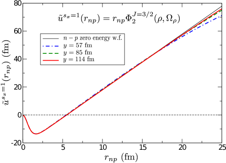
Figure 1: (Color online) Wave function $\tilde{u}^{s_{x}=1}(r_{np})$ obtained from the lowest breakup angular eigenfunction $\Phi_{2}^{J=1/2}(\rho,\Omega_{\rho})$ for the $n-d$ case with total angular momentum $J=3/2$ (see text), and for three different fixed values of the Jacobi coordinate $y$, 57 fm (thick dot-dashed), 85 fm (thick dashed), and 114 fm (thick solid). The thin solid line is the zero energy neutron-proton wave function $u^{s_{x}=1}$ introduced in Eq.(32).

To illustrate this point we take the $n-d$ case with total spin $J=3/2$ as an example. In this case, according to Eq.(E), for the geometries having $\alpha\approx 0$ ($x\ll y$) and assuming relative $s$-waves between the particles we should get:

$$\Phi_{n}^{J=3/2}(\rho,\Omega_{\rho})\stackrel{{\scriptstyle\rho\rightarrow\infty}}{{\rightarrow}}\frac{u^{s_{x}=1}}{r_{np}}$$ (32)

for all the angular eigenfunctions associated to breakup channels ($n>1$), where $u^{s_{x}=1}/r_{np}$ is the zero energy neutron-proton wave function, and $r_{np}$ is the relative distance between the neutron and the proton. In Fig.1 we plot the function $\tilde{u}^{s_{x}=1}(r_{np})=r_{np}\Phi_{2}^{J=3/2}(\rho,\Omega_{\rho})$ as a function $r_{np}$ for three fixed values of the Jacobi coordinate $y$, 57 fm (dot-dashed curve), 85 fm (dashed curve), and 114 fm (solid curve). Obviously, the larger the value of $y$ the smaller the value of the hyperangle $\alpha$ associated to a given $r_{np}$, and therefore the more should the function $\tilde{u}^{s_{x}=1}$ approach the zero-energy two-body function $u^{s_{x}=1}$ given in Eq.(32), which is shown in Fig.1 by the thin solid line. The expected behavior is what we observe in the figure, where, as we can see, for $y=114$ fm the function $\tilde{u}^{s_{x}=1}$ (thick solid curve) matches the two-body wave function $u^{s_{x}=1}$ (thin solid curve) pretty well up to almost 20 fm (the thin solid curve has been scaled to fit the same minimum as $\tilde{u}^{s_{x}=1}$).

The zero-energy two-body wave function is linear in the relative radial coordinate (see Fig.1), and therefore proportional to $\sin\alpha_{q}$. The reconstruction of this behavior by use of an expansion in terms of $\cos 2\alpha_{q}$, as in the expansion given in Eq.(II.3), requires in principle infinitely many terms. Accordingly, as $\alpha_{q}\rightarrow 0$ the number of adiabatic terms needed to get a convergent value for $A_{s_{x_{p}}}(p)$ increases without limit. Hence, Eq.(II.3) is not operative in this particular situation.

To overcome this problem we shall develop in this section an alternative expression for the transition amplitude where the adiabatic expansion in Eq.(II.3), in terms of the coefficients $C_{Ks_{x_{q}}}^{(n)}$, does not enter explicitly. This procedure will be more expensive from a numerical point of view, but more accurate in the kinematic regions where $\alpha_{\kappa}\approx 0$. The starting point here is the well known expansion of the three-body plane wave in terms of the hyperspherical harmonics:

$$e^{i({\small\bm{k}}_{x}\cdot{\small\bm{x}}+{\small\bm{k}}_{y}\cdot{\small\bm{y}})}|\sigma_{i}\sigma_{j}\sigma_{k}\rangle=$$

$$\frac{(2\pi)^{3}}{(\kappa\rho)^{2}}\sum_{JM}\sum_{[K]}i^{K}J_{K+2}(\kappa\rho){\cal Y}_{[K]}^{JM}(\Omega_{\rho})\langle\sigma_{i}\sigma_{j}\sigma_{k}|{\cal Y}_{[K]}^{JM*}(\Omega_{\kappa}),$$

where ${\cal Y}_{[K]}^{JM}$ is a HH function coupled to a three-body spin function nie01 . All the quantum numbers are collected into the set $[K]\equiv\{K,\ell_{x},\ell_{y},L,s_{x},S\}$. On the other hand, the angular eigenfunctions in the adiabatic expansion corresponding to breakup channels ($n>1$) are, asymptotically, linear combination of hyperspherical harmonics. The two bases can be formally related as

$${\cal Y}_{[K]}^{JM}(\Omega)=\sum_{n>1}\langle\Phi^{JM}_{n}(\Omega)|{\cal Y}_{[K]}^{JM}(\Omega)\rangle\Phi^{JM}_{n}(\Omega),$$ (34)

with the sum over $n$ restricted to those channels associated to the grand-angular quantum number $K$. Replacing in Eq.(II.4) we obtain

$$e^{i({\small\bm{k}}_{x}\cdot{\small\bm{x}}+{\small\bm{k}}_{y}\cdot{\small\bm{y}})}|\sigma_{i}\sigma_{j}\sigma_{k}\rangle=$$

$$\frac{(2\pi)^{3}}{(\kappa\rho)^{2}}\sum_{JM}\sum_{n>1}i^{K}J_{K+2}(\kappa\rho)\Phi_{n}^{JM}(\Omega_{\rho})\langle\sigma_{i}\sigma_{j}\sigma_{k}|\Phi_{n}^{JM}(\Omega_{\kappa})\rangle^{*},$$

where we have used that $\sum_{[K]}\langle\Phi^{JM}_{n}|{\cal Y}_{[K]}^{JM}\rangle\langle{\cal Y}_{[K]}^{JM}|\Phi^{JM}_{n^{\prime}}\rangle=\delta_{nn^{\prime}}$.

As shown in Ref.gar12 , the regular outgoing wave functions for the breakup channels are given by:

$$F_{n}=\sqrt{\frac{\pi}{2}}\frac{1}{\rho^{2}}J_{K+2}(\kappa\rho)\Phi_{n}^{JM}(\Omega_{\rho}).$$ (36)

Therefore Eq.(II.4) can be written in terms of $F_{n}$, and in particular it can be used to write the following matrix element:

$$\langle\Psi_{1}^{JM}|\hat{\cal H}-E|e^{i({\small\bm{k}}_{x}\cdot{\small\bm{x}}+{\small\bm{k}}_{y}\cdot{\small\bm{y}})}|\sigma_{i}\sigma_{j}\sigma_{k}\rangle\rangle=$$

$$\frac{(2\pi)^{3}}{\kappa^{2}}\sqrt{\frac{2}{\pi}}\sum_{n>1}i^{K}\langle\Psi_{1}^{JM}|\hat{\cal H}-E|F_{n}\rangle\langle\sigma_{i}\sigma_{j}\sigma_{k}|\Phi_{n}^{JM}(\Omega_{\kappa})\rangle^{*},$$

where $\hat{\cal H}$ is the three-body hamiltonian, $E$ is the total three-body energy, and $\Psi_{1}^{JM}$ is the three-body wave function corresponding to the incoming 1+2 channel labeled by 1.

In Ref.gar12 it was also shown that the ${\cal K}$-matrix for a breakup process can be obtained through two integral relations that provide the two matrices $A$ and $B$, such that the ${\cal K}$-matrix of the reaction takes the form ${\cal K}=-{A}^{-1}B$. In particular, the $ij$-term of each of these two matrices is given by:

$$A_{ij} = -\frac{2m}{\hbar^{2}}\langle\Psi_{i}^{JM}|\hat{\cal H}-E|G_{j}\rangle$$ (38)

$$B_{ij} = \frac{2m}{\hbar^{2}}\langle\Psi_{i}^{JM}|\hat{\cal H}-E|F_{j}\rangle,$$ (39)

where $G_{j}$ is defined as $F_{j}$, Eq.(36), but replacing the regular Bessel function $J_{K+2}$ by the irregular Bessel function $Y_{K+2}$.

Use of Eq.(39) permits to write Eq.(II.4) as:

$$\langle\Psi_{1}^{JM}|\hat{\cal H}-E|e^{i({\small\bm{k}}_{x}\cdot{\small\bm{x}}+{\small\bm{k}}_{y}\cdot{\small\bm{y}})}|\sigma_{i}\sigma_{j}\sigma_{k}\rangle\rangle=$$

$$\frac{(2\pi)^{3}}{\kappa^{2}}\sqrt{\frac{2}{\pi}}\frac{\hbar^{2}}{2m}\sum_{n>1}i^{K}B_{1n}\langle\sigma_{i}\sigma_{j}\sigma_{k}|\Phi_{n}^{JM}(\Omega_{\kappa})\rangle^{*},$$

where it is important to keep in mind that $1$ refers to the incoming channel (1+2 channel) and $n$ refers to the breakup channels (therefore $n>1$).

Note that the matrix element in Eq.(II.4) is just the first component of a column vector whose $i$-th term is given by $\langle\Psi_{i}^{JM}|\hat{\cal H}-E|\mbox{plane wave}\rangle$ ($i=1,\cdots,N$, where $N$ is the number of adiabatic channels included in the calculation) where for $i>2$ the wave functions $\Psi_{i}^{JM}$ describe scattering processes with three ingoing particles. If we multiply from the left such column vector by any $N\times N$ matrix $M$, the result would be a new column vector whose first term would be given by Eq.(II.4) but replacing $B_{1n}$ by $\left(M\cdot B\right)_{1n}$. Therefore, if we take $M=A^{-1}$, the first component of the new vector will be given by Eq.(II.4) but replacing $B_{1n}$ by $(A^{-1}B)_{1n}$, which is nothing but $-{\cal K}_{1n}$.

For the same reason, since ${\cal K}=-i({\cal S}+\mathbbm{I})^{-1}({\cal S}-\mathbbm{I})$, if we multiply from the left the new column vector by $({\cal S}+\mathbbm{I})$, the new matrix element in Eq.(II.4) would be given not in terms of ${\cal K}_{1n}$, but in terms of $({\cal S}-\mathbbm{I})_{1n}$, which reduces to ${\cal S}_{1n}$ in our case, where $1$ refers to the $1+2$ incident channel and $n$ corresponds to outgoing breakup channels ($n>1$).

Summarizing, the first step is to compute the $A$ and $B$ matrices as described in Ref.gar12 , from which the ${\cal S}-$matrix of the reaction can be obtained. Successively a proper normalized scattering state is constructed according to:

$$\Psi^{JM}\rightarrow({\cal S}+\mathbbm{I})A^{-1}\Psi^{JM},$$ (41)

and once this is done the matrix element given in Eq.(II.4) transforms into:

$$\langle\Psi_{1}^{JM}|\hat{\cal H}-E|e^{i({\small\bm{k}}_{x}\cdot{\small\bm{x}}+{\small\bm{k}}_{y}\cdot{\small\bm{y}})}|\sigma_{i}\sigma_{j}\sigma_{k}\rangle\rangle=$$

$$i\frac{(2\pi)^{3}}{\kappa^{2}}\sqrt{\frac{2}{\pi}}\frac{\hbar^{2}}{2m}\sum_{n>1}i^{-K}{\cal S}_{1n}\langle\sigma_{i}\sigma_{j}\sigma_{k}|\Phi_{n}^{JM}(\Omega_{\kappa})\rangle^{*},$$

where the replacement of $i^{K}$ by $i^{-K}$ is irrelevant, since the difference is a factor $i^{2K}=(-1)^{K}$, which is either 1 for positive parity states ($K$ even for all $n$) or $-1$ for negative parity states ($K$ odd for all $n$). In any case, this is not playing any role, since the calculation of the cross section will contain the square of the matrix element above.

In Eq.(II.4) the angular function $\langle\sigma_{i}\sigma_{j}\sigma_{k}|\Phi_{n}(\Omega_{\kappa})\rangle$ is just the Fourier transform of Eq.(II.3), whose analytical form is exactly the same as in Eq.(II.3) but with the angles understood in momentum space (asymptotically the hyperangles in coordinate and momentum space are the same).

Comparing Eqs.(II.3) and (II.4), we can identify the breakup transition amplitude as:

$$A_{\sigma_{d}\sigma_{n}}^{\sigma_{i}\sigma_{j}\sigma_{k}}=\frac{\pi}{\sqrt{2}}\frac{\kappa^{2}}{\sqrt{\kappa k_{y}}}\frac{1}{(2\pi)^{3}}\left(\frac{\mu_{x}}{m}\right)^{3/4}e^{i\frac{\pi}{4}}\frac{2m}{\hbar^{2}}$$

$$\times\sum_{JM}\langle s_{d}\sigma_{d}s_{p}\sigma_{p}|JM\rangle\langle\Psi_{1}^{JM}|\hat{\cal H}-E|e^{i({\small\bm{k}}_{x}\cdot{\small\bm{x}}+{\small\bm{k}}_{y}\cdot{\small\bm{y}})}|\sigma_{i}\sigma_{j}\sigma_{k}\rangle\rangle.$$

Since the plane wave is the solution of the free hamiltonian, the matrix element in Eq.(II.4) is actually the sum of three matrix elements, each of them involving one of the three two-body potentials. In turn, each of these three matrix elements is more easily treated in the Jacobi set such that the potential depends on the $\bm{x}$ coordinate only. In other words, we can write:

$$\langle\Psi_{1}^{JM}|\hat{\cal H}-E|e^{i({\small\bm{k}}_{x}\cdot{\small\bm{x}}+{\small\bm{k}}_{y}\cdot{\small\bm{y}})}|\sigma_{i}\sigma_{j}\sigma_{k}\rangle\rangle=$$ (44)

$$\sum_{q=1}^{3}\langle\Psi_{1}^{JM}|V_{q}(x_{q})|e^{i({\small\bm{k}}_{x_{q}}\cdot{\small\bm{x}_{q}}+{\small\bm{k}}_{y_{q}}\cdot{\small\bm{y}_{q}})}|\sigma_{i}\sigma_{j}\sigma_{k}\rangle\rangle,$$

where $V_{q}(x_{q})$ is the two-body potential between the two particles connected by the Jacobi coordinate $\bm{x}_{q}$.

If we now consider that

$$\langle\Psi_{1}^{JM}|V_{q}(x_{q})|e^{i({\small\bm{k}}_{x_{q}}\cdot{\small\bm{x}_{q}}+{\small\bm{k}}_{y_{q}}\cdot{\small\bm{y}_{q}})}|\sigma_{i}\sigma_{j}\sigma_{k}\rangle\rangle=$$

$$\sum_{s_{x_{q}}}\langle\Psi_{1}^{JM}|V_{q}(x_{q})|e^{i({\small\bm{k}}_{x_{q}}\cdot{\small\bm{x}_{q}}+{\small\bm{k}}_{y_{q}}\cdot{\small\bm{y}_{q}})}|\chi_{s_{x_{q}}s_{y_{q}}}^{JM}\rangle\rangle\langle\chi_{s_{x_{q}}s_{y_{q}}}^{JM}|\sigma_{i}\sigma_{j}\sigma_{k}\rangle,$$

where $s_{x_{q}}$ is the spin of the two-body system connected by the $\bm{x}_{q}$ Jacobi coordinate, we can then, by use of Eqs.(44) and (II.4), write the transition amplitude in Eq.(II.4) exactly as given in Eq.(II.3), where now

$$A_{s_{x_{q}}}(q)=\frac{\pi}{\sqrt{2}}\frac{\kappa^{2}}{\sqrt{\kappa k_{y_{q}}}}\frac{1}{(2\pi)^{3}}\left(\frac{\mu_{x}}{m}\right)^{3/4}e^{i\frac{\pi}{4}}$$

$$\times\frac{2m}{\hbar^{2}}\langle\Psi_{1}^{JM}|V_{q}(x_{q})|e^{i({\small\bm{k}}_{x_{q}}\cdot{\small\bm{x}_{q}}+{\small\bm{k}}_{y_{q}}\cdot{\small\bm{y}_{q}})}|\chi_{s_{x_{q}}s_{y_{q}}}^{J}\rangle\rangle.$$

Thus, Eq.(II.4) permits to obtain Eq.(II.3), and therefore the cross sections in Eqs.(II.2) and (14). Contrary to what happens in Eq.(II.3), Eq.(II.4) does not contain any expansion of the outgoing wave, and in principle the infinitely many breakup adiabatic terms are included. The discussion of the calculation of the matrix element contained in Eq.(II.4) is given in the next section.

III Calculation of the breakup integral relation using the HA formalism

Let us denote the matrix element to be computed as:

$$M_{s_{x_{i}}}(\bm{k}_{x_{i}},\bm{k}_{y_{i}})=\langle\Psi_{1}^{JM}|V_{i}(x_{i})|e^{i({\small\bm{k}}_{x_{i}}\cdot{\small\bm{x}_{i}}+{\small\bm{k}}_{y_{i}}\cdot{\small\bm{y}_{i}})}|\chi_{s_{x_{i}}s_{y_{i}}}^{JM}\rangle\rangle.$$ (47)

The three-body wave function $\Psi_{1}^{JM}$ is expanded in terms of the adiabatic angular eigenfunctions, which in turn are expanded in terms of the hyperspherical harmonics (see also Refs. rom11 ; gar12 ):

$$\Psi_{1}^{JM}(\bm{x}_{i},\bm{y}_{i})=$$

$$\frac{1}{\rho^{5/2}}\sum_{n}f_{n1}(\rho)\sum_{[K]}C^{(n)}_{[K]}(\rho){\cal Y}_{[K]}^{JM}(\Omega_{i})$$

where the coefficients $C^{(n)}_{[K]}$ reduce to $C^{(n)}_{K,s_{x_{i}}}$ in the case of $s$-waves and where we have selected the $i$ arrangement of the Jacobi coordinates to construct the three-body HH-spin functions ${\cal Y}_{[K]}^{JM}$. It should be noticed that it is convenient to expand the three-body wave function $\Psi_{1}^{JM}$ in the set $i$ of Jacobi coordinates in which the coordinate $\bm{x}_{i}$ is the same appearing in the interaction potential, as given in Eq.(47). Therefore for each of the three integrals given in Eq.(44), the corresponding set of Jacobi coordinates is used.

Inserting the above expansion into Eq.(47), we get that the matrix element takes the form (the index $i$ will be omitted from now on and we consider $s$-wave only):

$$M_{s_{x}}(\bm{k}_{x},\bm{k}_{y})=\frac{1}{4\pi}\int d^{3}xd^{3}y\frac{1}{\rho^{5/2}}\sum_{n}f_{n1}(\rho)\sum_{K}C^{(n)}_{K,s_{x}}(\rho)N_{K}P_{\nu}^{(\frac{1}{2},\frac{1}{2})}(\cos 2\alpha)\langle\chi_{s_{x}s_{y}}^{JM}|V(x)|\chi_{s_{x}s_{y}}^{JM}\rangle e^{i({\small\bm{k}}_{x_{i}}\cdot{\small\bm{x}_{i}}+{\small\bm{k}}_{y_{i}}\cdot{\small\bm{y}_{i}})}$$ (49)

where the two-body potential is assumed not to mix different $s_{x}$-values.

Keeping in mind that the input in our calculation will be the directions of the momenta of two of the outgoing particles and that, as already shown, for each value of the arclength $S$ it is possible to construct the full momenta of the three particles after the breakup, these three momenta permit us to construct $\bm{k}_{x}$ and $\bm{k}_{y}$, and the matrix element in Eq.(49) can then be computed as a function of the arclength $S$.

Note also that in Eq.(49), since only $s$-waves are assumed to contribute, the full dependence of the integrand on $\Omega_{x}$ and $\Omega_{y}$ is contained in the exponential. The integration over $\Omega_{x}$ and $\Omega_{y}$ can then be made analytically, leading to the expression:

$$\int d\Omega_{x}d\Omega_{y}(\cos({\small\bm{k}}_{x}\cdot{\small\bm{x}}+{\small\bm{k}}_{y}\cdot{\small\bm{y}})+i\sin({\small\bm{k}}_{x}\cdot{\small\bm{x}}+{\small\bm{k}}_{y}\cdot{\small\bm{y}}))=$$ (50)

$$(2\pi)^{2}\frac{4\sin(k_{x}x)\sin(k_{y}y)}{k_{x}xk_{y}y},$$

which is real (the integral involving the sinus is just zero).

The remaining integral over $x$ and $y$ has to be performed numerically:

$$M_{s_{x}}(k_{x},k_{y})=4\pi\int dxdy\frac{xy}{\rho^{5/2}}\sum_{n}f_{n1}(\rho)\sum_{K}C^{(n)}_{K,s_{x}}(\rho)N_{K}P_{\nu}^{(\frac{1}{2},\frac{1}{2})}(\cos 2\alpha)\langle\chi_{s_{x}s_{y}}^{JM}|V(x)|\chi_{s_{x}s_{y}}^{JM}\rangle\frac{\sin(k_{x}x)\sin(k_{y}y)}{k_{x}k_{y}}.$$ (51)

As we can see, the dependence on the directions of $\bm{k}_{x}$ and ${\bm{k}_{y}}$ has disappeared. The dependence on the momenta is only through $k_{x}=\kappa\sin\alpha_{\kappa}$ and $k_{y}=\kappa\cos\alpha_{\kappa}$, where $\kappa=\sqrt{2mE/\hbar^{2}}$ and where $E$ is the three-body energy above threshold. It is important not to get confused with $\alpha$ ($=\arctan x/y$), which is a variable in coordinate space to be integrated away, and $\alpha_{\kappa}$ ($=\arctan k_{x}/k_{y}$), which is a variable in momentum space, and which takes a well defined value for each value of the arclength $S$.

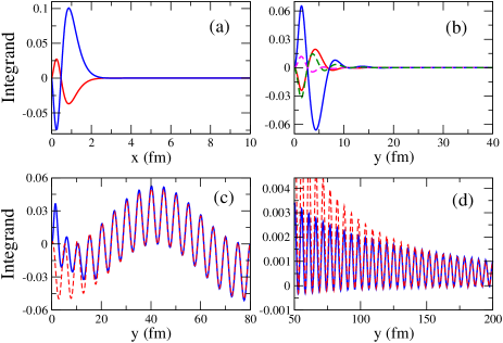
Figure 2: (Color online) Typical integrand of Eq.(51) obtained for the $n-d$ reaction and for the following different cases: (a) as a function of $x$ for two fixed values of $y$, (b) as a function of $y$ ($x$-coordinate integrated away) and $n$ being a 1+2 channel for the neutron-neutron potential (solid curves), and for the neutron-proton potential with $s_{x}=0$ (dashed curves), (c) as a function of $y$ ($x$-coordinate integrated away) and $n$ being a 1+2 channel for the neutron-proton potential and $s_{x}=1$, (d) as a function of $y$ ($x$-coordinate integrated away) for $n$ being a breakup channel. In (c) and (d) the dashed curves are the asymptotic matching given by Eq.(54) and (III.0.2), respectively.

The integral over $x$ is limited by the short-range character of the potential $V(x)$. Therefore the numerical computation of the integral does not present any particular difficulties. In Fig. 2a we show two examples of the typical behavior of the integrand as a function of $x$ for two arbitrary fixed values of $y$. The curves correspond to the $n-d$ breakup reaction whose details will be given later on. They have been obtained for two fixed values of the $y$-coordinate. As we can see, the function becomes basically zero for rather small values of $x$.

The integral over $y$ is however more complicated. In general, the integrand does not fall off exponentially at large distances, and its calculation is therefore more delicate. We can distinguish two different cases depending on the asymptotic behavior of the $f_{n1}(\rho)$ radial wave function, i.e., when $n$ is associated to the 1+2 channel or to a breakup channel. In the following we discuss the two cases.

III.0.1 Index $n$ corresponding to a 1+2 channel

When $n$ labels a 1+2 channel ($n=1$ in our case), the corresponding Faddeev amplitudes of the angular function $\Phi_{n}^{JM}(\rho,\Omega_{\rho})$ behave at large distances as given by Eq.(E), which reduces to

$$\Phi_{n}^{JM}(\rho,\Omega_{i})\rightarrow\rho^{3/2}\frac{1}{4\pi}\Psi_{d}|\chi_{s_{d}s_{y}}^{JM}\rangle,$$ (52)

when only $s$-waves are involved. In this expression $\Psi_{d}$ is the bound two-body wave function of the dimer associated to the 1+2 channel $n$ and $s_{d}$ is the spin of the dimer.

Having this in mind, we can observe that the sum on the HH index $K$ in Eq.(51) can be reconstructed for $n=1$ (1+2 channel) as

$$\frac{1}{4\pi}\sum_{K}C^{(n)}_{K,s_{x}}(\rho)N_{K}P_{\nu}^{(\frac{1}{2},\frac{1}{2})}(\cos 2\alpha)\langle\chi_{s_{x}s_{y}}^{JM}|V(x)|\chi_{s_{x}s_{y}}^{JM}\rangle=$$

$$\langle\Phi_{1}^{JM}(\rho,\Omega_{\rho})|V(x)|\chi_{s_{x}s_{y}}^{JM}\rangle=$$

$$\sum_{i}\langle\Phi_{1}^{JM}(\rho,\Omega_{i})|V(x)|\chi_{s_{x}s_{y}}^{JM}\rangle.$$ (53)

The last expression shows that, at large distances, the integrand in Eq.(51) contains explicitly the dimer wave function in the different Jacobi permutations. Two different possibilities appear: the potential and the dimer depend on Jacobi coordinates belonging to two different permutations, for example $\bm{x}_{i}$ and $\bm{x}_{j}$. In this case the integral in Eq.(51) has an exponential fall off in both coordinates, $x$ and $y$. In fact, when the two-body potential refers to the two particles that do not form the dimer (for instance the $V_{nn}(x)$ potential in the $n-d$ case), large values of $y$ would correspond to large distances between the third particle and the one with which that third particle forms the dimer (large neutron-proton distance in the $n-d$ case). Thus, for sufficiently large values of $y$ the integrand should be zero due to the presence of the bound dimer wave function, which is now basically associated to the $y$-coordinates at large distances. Taking again the $n-d$ case as an illustration, the solid curves in Fig.2b correspond to the integrand of Eq.(51) as a function of $y$ for two different values of the arclength $S$ (after integrating away the $x$-coordinate) for the case of the neutron-neutron potential. As shown in the figure, the integrand in the $y$ coordinate dies pretty fast, and it is negligible already at distances of even less than 40 fm.

A similar case arises when the interaction is the one giving rise to the dimer (the neutron-proton potential in the $n-d$ case) and $s_{x}$ is different to the spin of the bound dimer ($s_{x}=0$ in the $n-d$ case). The reason now is that the coefficients $C_{K,s_{x}\neq s_{d}}(\rho)$ in Eq.(51) go to zero for large values of the hyperradius (as shown in Eq.(52), asymptotically only the terms with $s_{x}=s_{d}$ survive). This case is illustrated in Fig.2b by the dashed lines, which correspond to the $n-d$ case, and which show that also in this case the integrand goes to zero rather fast. Therefore, in the particular cases shown in Fig.2b the numerical computation of the integral in the both variables, $x$ and $y$, do not present particular problems.

A different situation appears when the potential in Eq.(51) and the dimer depend on the same variable $\bm{x}$ and when $s_{x}=s_{d}$ (neutron-proton potential and $s_{x}=1$ in the $n-d$ case). In this case the the $y$-coordinate integrand in Eq.(51) does not vanish exponentially and a particular analysis of the integrand tail has to be performed.

It is well known gar12 that the large distance behavior of $f_{n1}(\rho)$, for $n$ being a 1+2 channel, is given by:

$$f_{n1}(\rho)\rightarrow C\sin(k_{y}^{(n)}y)+D\cos(k_{y}^{(n)}y),$$ (54)

where $C$ and $D$ are complex numbers (the $f_{n1}$-functions are complex), and $(k_{y}^{(n)})^{2}=2m(E-E_{n})/\hbar^{2}$, where $E_{n}$ is the binding energy of the dimer present in the 1+2 channel associated to the adiabatic term $n$.

Therefore, using Eqs.(54) and (52) it is clear that the integrand in Eq.(51) is asymptotically separable into $x$ and $y$ coordinates, and the integrand of the $y$ part goes like:

$$\mbox{Integrand}(y)\rightarrow$$

$$C\sin(k_{y}^{(n)}y)\sin(k_{y}y)+D\cos(k_{y}^{(n)}y)\sin(k_{y}y),$$

where $C$ and $D$ are complex constants, and where we have used that, since $x$ is restricted to small values, then $y/\rho\rightarrow 1$.

This behavior is shown in Fig.2c again for the $n-d$ case. The solid curve is the integrand in the $y$-coordinate obtained numerically for some value of the arclength $S$, and the dashed curve is the matching with the expression in Eq.(III.0.1). As shown in the figure the matching is pretty good for distances already of about 30-40 fm.

Therefore an easy way of computing the integral over $y$ in Eq.(51) (for the two-body potential giving rise to the dimer and $s_{x}=s_{d}$) is to do it numerically after subtracting the asymptotic behavior given in Eq.(III.0.1), i.e., integrating numerically the difference between the solid and the dashed curves in Fig.2c, which dies asymptotically sufficiently fast, and afterward add the analytical integral of Eq.(III.0.1) from $y=0$ to $\infty$. This analytical integral can be easily made by using that:

$$\int_{0}^{\infty}\sin(k_{y}^{(n)}y)\sin(k_{y}y)dy=\lim_{a\rightarrow 0}\left[\int_{0}^{\infty}e^{-ay}\sin(k_{y}^{(n)}y)\sin(k_{y}y)dy\right]=0;(a>0)$$ (56)

$$\int_{0}^{\infty}\cos(k_{y}^{(n)}y)\sin(k_{y}y)dy=\lim_{a\rightarrow 0}\left[\int_{0}^{\infty}e^{-ay}\cos(k_{y}^{(n)}y)\sin(k_{y}y)dy\right]=\frac{k_{y}}{(k_{y})^{2}-(k_{y}^{(n)})^{2}};(a>0)$$ (57)

where we have to remember that $k_{y}=\kappa\cos\alpha_{\kappa}$ and $k_{y}^{(n)}=\sqrt{2m(E-E_{n})/\hbar^{2}}$, which are always different ($E_{n}<0$).

III.0.2 Index $n$ corresponding to a breakup channel

Due to the short-range character of the potential, the $x$-values are in any case restricted to relatively small values, no matter the character of the channel $n$ in Eq.(51). For this reason, even if $n$ corresponds to a breakup channel, the large distance behavior of the integrand is given by contributions fulfilling that $y\gg x$ (or, in other words, $\rho\approx y$).

Also, for a breakup channel $n$, the coefficients $C_{K,s_{x}}^{(n)}(\rho)$ go to constant values (the angular eigenfunctions $\Phi_{n}^{J}$ become just a linear combination of hyperspherical harmonics, see Eq.(II.3)), and the Jacobi Polynomials $P_{\nu}^{(\frac{1}{2},\frac{1}{2})}(\cos 2\alpha)$ contained in the hyperspherical harmonics go also to the constant value $P_{\nu}^{(\frac{1}{2},\frac{1}{2})}(1)$.

Finally, the general behavior at large distances of the radial functions $f_{n1}(\rho)$ is given by a linear combination of the Hankel functions of first and second order gar12 , which means that their asymptotic behavior is given by:

$$f_{n1}(\rho)\rightarrow\sum_{m=0}^{M}\frac{C_{m}\sin(\kappa y)+D_{m}\cos(\kappa y)}{y^{m}},$$ (58)

where we have already replaced $\rho$ by $y$.

Therefore, when $n$ is associated to a breakup channel, the $y$-part of the integrand in Eq.(51) goes asymptotically as:

$$\mbox{Integrand}(y)\rightarrow$$

$$\sum_{m=0}^{M}\left(\frac{C_{m}\sin(\kappa y)\sin(k_{y}y)}{y^{m+3/2}}+\frac{D_{m}\cos(\kappa y)\sin(k_{y}y)}{y^{m+3/2}}\right),$$

where, again, the constants $C_{m}$ and $D_{m}$ are complex and $k_{y}=\kappa\cos\alpha_{\kappa}$. Obviously, the higher the value of $M$, the lower the value of $y$ at which the matching with the numerical integrand is obtained.

Thus, for outgoing breakup channels, the $y$-part of the integral in Eq.(51) goes to zero asymptotically as $1/y^{3/2}$. It could then seem that such integral could be done numerically without much trouble. However, the fall off is not fast enough, and at relatively large distances the integrand is not really negligible. Taking again the $n-d$ case as an example, this is shown in Fig.2d, where the blue curve is the integrand in Eq.(51) as a function of $y$ for some value of the arclength $S$ and for $n$ being one of the breakup channels ($n>1$). At a distance of about 200 fm the integrand is not at all negligible, in fact the amplitude of the oscillations shown in the figure are still about 10% of the maximum computed amplitude. The dashed curve shows the matching given by Eq.(III.0.2) and $M=0$. It is clear that this matching is less accurate than the one shown in Fig.2c, and the agreement now with the true integrand is observed much farther, at 150 fm at least.

Therefore, due to the too slow fall off of the integrand, it is convenient to integrate numerically up to some $y_{\mbox{\scriptsize max}}$ value at which the matching with the asymptotic behavior in Eq.(III.0.2) has already been achieved, and to perform analytically the integrand from $y_{\mbox{\scriptsize max}}$ up to $\infty$. These analytical integrations involve the so-called Fresnel integrals, and they can be performed as indicated in appendix F.

IV The $n-d$ case

In this section we shall compute the cross sections for neutron-deuteron breakup. This choice is made in order to compare to the benchmark calculations given in fri95 . Following this reference, we have chosen the Malfliet-Tjon-I-III model $s$-wave nucleon-nucleon potential fri90 , which for the triplet and singlet cases takes the form:

$$V_{t}(r)=\frac{1}{r}\left(-626.885e^{-1.55r}+1438.72e^{-3.11r}\right),$$ (60)

and

$$V_{s}(r)=\frac{1}{r}\left(-513.968e^{-1.55r}+1438.72e^{-3.11r}\right),$$ (61)

respectively, and where the $r$ is in fm, the potential in MeV, and $\hbar^{2}/m=41.47$ MeV fm². In our calculations $m$ is taken as the normalization mass in the definitions of the Jacobi coordinates given in Eqs.(3) to (6).

In the first part of this section we summarize the results obtained in Ref.gar12 for the ${\cal S}$-matrix after application of the integral relations. We continue with the cross sections obtained from the adiabatic expansion of the transition amplitude in Eq.(II.3), and the inaccuracies corresponding to some particular geometries are analyzed. In the last part of the section we show how the use of the transition amplitude given by Eq.(II.4) corrects the cross sections in the regions were the inaccuracies were observed.

IV.1 ${\cal S}$-matrix

The details concerning the integral relations formalism applied to the description of breakup 1+2 reactions are given in Ref.gar12 . This method permits to extract the ${\cal S}$-matrix of the reaction from the internal part of the wave function. When this wave function is obtained by means of the adiabatic expansion method, the pattern of convergence of the ${\cal S}$-matrix is similar to the one obtained with the same method for bound states.

In gar12 the integral relations method is applied to the $n-d$ reaction. Only $s$-waves are considered in the calculation, which implies that only two different total angular momenta are possible, the quartet case ($J$=3/2), for which only the triplet $s$-wave potential in Eq.(60) enters, and the doublet case ($J$=1/2), for which both the singlet and the triplet potentials contribute.

The unitarity of the ${\cal S}$- matrix implies that given an incoming channel, for instance, channel 1 ($n-d$ channel), we have that $\sum_{n=1}^{\infty}|{\cal S}_{1n}|^{2}=1$, or in other words:

$$\sum_{n=2}^{\infty}|{\cal S}_{1n}|^{2}=1-|{\cal S}_{11}|^{2},$$ (62)

which means that an accurate calculation of the elastic term ${\cal S}_{11}$ amounts to an accurate calculation of the infinite summation of the $|{\cal S}_{1n}|^{2}$ terms ($n>1$) corresponding to the breakup channels, and therefore allowing the calculation of the total breakup cross section given in Eq.(2).

The complex value of ${\cal S}_{11}$ can be written in terms of a complex phase shift $\delta$ as

$${\cal S}_{11}=e^{2i\delta}=e^{-2\mbox{\scriptsize Im}(\delta)}e^{2i\mbox{Re}(\delta)}=|{\cal S}_{11}|e^{2i\mbox{Re}(\delta)}.$$ (63)

The value of $|{\cal S}_{11}|^{2}$ gives the probability of elastic neutron-deuteron scattering, and $|{\cal S}_{11}|$ is what usually referred to as the inelasticity parameter (denoted by $\eta$ in fri95 ; fri90 ). Obviously, the closer the inelasticity to 1 the more elastic the reaction. In fact, for energies below the breakup threshold the phase-shift is real and $|{\cal S}_{11}|=1$.

Table 1: Inelasticity parameter $|{\cal S}_{11}|$ for the neutron-deuteron scattering for two different laboratory neutron beam energies (14.1 MeV and 42.0 MeV) for the doublet and quartet cases. The value of $K_{\mbox{\scriptsize max}}$ is the $K$-value associated to the last adiabatic potential included in the calculation. The last row gives the value quoted in Ref.fri95 .

$K_{\mbox{\scriptsize max}}$	Doublet		Quartet
	14.1 MeV	42.0 MeV	14.1 MeV	42.0 MeV
4	0.4662	0.4929	0.9794	0.8975
8	0.4637	0.4993	0.9784	0.9026
12	0.4640	0.5014	0.9783	0.9030
16	0.4643	0.5019	0.9782	0.9031
20	0.4644	0.5021	0.9782	0.9033
24	0.4645	0.5022	0.9782	0.9033
28	0.4645	0.5022	0.9782	0.9033
Ref.fri95	0.4649	0.5022	0.9782	0.9033

Table 2: The same as Table 1 for Re($\delta$).

$K_{\mbox{\scriptsize max}}$	Doublet		Quartet
	14.1 MeV	42.0 MeV	14.1 MeV	42.0 MeV
4	105.82	42.66	69.04	38.98
8	105.57	41.65	68.99	37.95
12	105.53	41.49	68.98	37.77
16	105.53	41.46	68.97	37.73
20	105.53	41.45	68.96	37.72
24	105.53	41.44	68.96	37.71
28	105.53	41.44	68.96	37.71
Ref.fri95	105.50	41.37	68.96	37.71

In tables 1 and 2 we quote the results given in gar12 for the inelasticity parameter $|{\cal S}_{11}|$ and the real part of the phase shift Re($\delta$), respectively. We have used the same two lab energies considered in Ref.fri95 , i.e., 14.1 MeV and 42.0 MeV. The value of $K_{\mbox{\scriptsize max}}$ given in the tables corresponds to the asymptotic grand-angular quantum number associated to the last adiabatic potential included in the adiabatic expansion.

As seen in the tables, the agreement with the results in Ref.fri95 is good. Actually, we obtain precisely the same result for the two incident energies in the quartet case, and a small difference clearly smaller than 0.1% in the doublet case. Furthermore, the pattern of convergence is rather fast, specially in the quartet case, for which already for $K_{\mbox{\scriptsize max}}=8$ we obtain a result that can be considered very accurate. In the doublet case the convergence is a bit slower, and a value of $K_{\mbox{\scriptsize max}}$ of about 16 is needed.

IV.2 Cross sections

Once the ${\cal S}$-matrix of the reaction has been computed, we can now obtain the transition matrix according to the expression in Eq.(II.3), and therefore also the expression Eq.(II.3) and the lab cross section in Eq.(14).

We shall consider an incident energy in the lab frame of $E_{in}^{(lab)}=14.1$ MeV and four different outgoing geometries specified by the polar angles $\theta_{1}$ and $\theta_{2}$ and the difference of azimuthal angles $\Delta\varphi=\varphi_{1}-\varphi_{2}$, where $(\theta_{1},\varphi_{1})$ and $(\theta_{2},\varphi_{2})$ describe the direction of the two outgoing neutrons. The four different cases are:

• Case 1: $\theta_{1}=45.0^{\circ}$, $\theta_{2}=53.56^{\circ}$, $\Delta\varphi=180^{\circ}$.

• Case 2: $\theta_{1}=35.0^{\circ}$, $\theta_{2}=44.0^{\circ}$, $\Delta\varphi=180^{\circ}$.

• Case 3: $\theta_{1}=60.06^{\circ}$, $\theta_{2}=53.10^{\circ}$, $\Delta\varphi=180^{\circ}$.

• Case 4: $\theta_{1}=51.02^{\circ}$, $\theta_{2}=51.02^{\circ}$, $\Delta\varphi=120^{\circ}$.

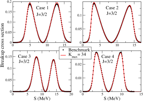
Figure 3: (Color online) Breakup cross sections, Eq.(14), as a function of the arclength $S$ for $n-d$ scattering in the quartet case ($J=3/2$) for a lab incident energy of 14.1 MeV. The cross sections are given in mb/(MeV sr²). The value of $K_{max}$ refers to the grand-angular quantum number $K$ associated to the last adiabatic term included in the expansion in Eq.(II.3). The four cases shown in the figure correspond to the four different directions of the outgoing neutrons specified in the text. The dotted curves are the result of the benchmark calculations given in Ref.fri95 .

The solid lines in Fig.3 show the computed cross section in Eq.(14) for the four cases given above for the quartet case ($J=3/2$). In the figure, $K_{max}$ refers to the asymptotic value of the grand-angular quantum number $K$ associated to last adiabatic term included in the expansion in Eq.(II.3). A value of $K_{max}=34$ amounts to including 18 adiabatic terms in the expansion. This is enough to reach convergence. In fact, the same calculation with $K_{max}=22$ (12 adiabatic terms) is basically indistinguishable from the curves shown in the figure. The cross sections given in the benchmark calculation in Ref.fri95 are shown by the dotted curves. As we can see, the results given in the benchmark calculation are nicely reproduced.

The corresponding cross sections for the doublet case ($J=1/2$) are shown by the dashed curves in the upper parts of Figs.4 and 5. When the contribution from the quartet state (Fig.3) is added, we get the total cross section given by the solid curves in the same figures. The doublet cross sections have been obtained with $K_{max}=34$, which for $J=1/2$ corresponds to inclusion of 35 adiabatic terms in the expansion of Eq.(II.3). Again, when $K_{max}$ is reduced to 22 (23 adiabatic terms) the computed curves can not be distinguished from the ones shown in the figure. As we can see, even if the computed cross sections have converged, there is a clear discrepancy with the benchmark calculation for Case 1, and, to a lower extent, for Case 2 (Fig.4). For Cases 3 and 4 (Fig.5) the agreement is reasonably good.

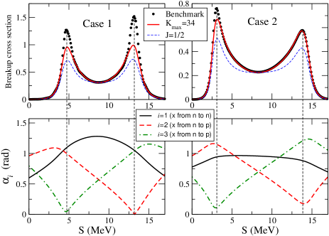
Figure 4: (Color online) Upper part: Total cross sections for the Cases 1 and 2 in the upper part of Fig.3. They are obtained by adding the quartet ($J=3/2$) contribution in Fig.3 and the doublet ($J=1/2$) contribution shown by the dashed curves. Lower part: For the same two cases, the corresponding values of $\alpha_{i}$ ($i=1,2,3$) as a function of the arclength $S$.

As anticipated in Section II.4, the discrepancy with the benchmark calculation appears in the $S$-regions corresponding to an outgoing kinematics where two of the particles have zero relative energy. This can be seen in Fig.4, where the lower part shows, as a function of the arclength $S$, the hyperangle $\alpha_{i}=\arctan(k_{x_{i}}/k_{y_{i}})$ for the Cases 1 and 2. The index $i=1$ corresponds to the Jacobi coordinates where $\bm{x}$ connects the two neutrons (solid curve), and the indices $i=2,3$ correspond to the Jacobi coordinates where $\bm{x}$ connects the proton and one of the neutrons (dashed and dot-dashed curves). For Case 1 (left part of the figure), we can see that $\alpha_{2}$ and $\alpha_{3}$ approach zero very much for $S$ slightly below 5 MeV and about 13 MeV. In these regions the proton and one of the neutrons move with relative zero (or very small) energy, and these are precisely the regions where the discrepancy with the benchmark calculation is observed. For Case 2, $\alpha_{2}$ and $\alpha_{3}$ do not approach zero as much as in Case 1, and the discrepancy with the benchmark calculation is now much smaller than in Case 1 (or even not visible, as it happens for the second peak of the cross section).

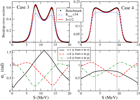
Figure 5: (Color online) The same as in Fig.4 for the Cases 3 and 4.

For completeness, we show in the lower part of Fig.5 the same as in Fig.4 but for Cases 3 and 4. Now the values of $\alpha_{i}$ do not reach zero for any $S$-value, and the agreement between our calculation and the benchmark is fine for all values of $S$.

As already mentioned, the problem is related to the fact that $\alpha_{i}\approx 0$ means two of the particles flying together with relative zero (or very small) energy, and the third particle moving far apart. The adiabatic expansion in Eq.(II.3) is then trying to reproduce the zero energy two-body wave function (which is proportional to $\sin\alpha$) in terms of a set of polynomials (the Jacobi polynomials) that have $\cos 2\alpha$ as argument. A correct description of the zero energy two-body wave function would require then infinitely many adiabatic terms.

As seen in Fig.3, the inaccuracy mentioned above for $\alpha_{i}\approx 0$ is not visible in the quartet case, where only triplet nucleon-nucleon components enter. However, as seen in Fig.4, where the contribution from the doublet has been added, the mismatch with the benchmark calculation becomes very significant. This is due to the fact that in the doublet case there is an important contribution from the singlet nucleon-nucleon components. This little difference is actually very relevant, because the singlet nucleon-nucleon potential has a rather large scattering length of about $-23$ fm, more than four times bigger (in absolute value) than the scattering length of the triplet nucleon-nucleon potential (of about $5$ fm). This means that the $s$-wave singlet nucleon-nucleon system has a pretty low-lying virtual state that favors the structure mentioned above of two nucleons flying together after the collision at a very low relative energy. For the case of the triplet nucleon-nucleon state the energy of the corresponding virtual state is about 20 times higher than in the singlet case (the virtual state energy is proportional to the inverse of the scattering length squared).

The solution suggested in order to solve the disagreement observed in Fig.4 is to skip the expansion of the outgoing wave in terms of the different adiabatic channels and compute instead the transition amplitude as given in Eq.(II.4), where the adiabatic expansion does not enter. The results obtained by using this alternative method are given in the following section.

IV.3 Corrections to the cross sections

The cross section in Eq.(15) is now computed making use of Eq.(II.4). The matrix element in this expression is given by Eq.(51), whose calculation requires using the techniques described is Sections III.0.1 and III.0.2 when integrating over the $y$-coordinate. For the case described in Fig.2c the integral over $y$ is made by integrating numerically the difference between the computed integrand and its analytic asymptotic behavior (difference between the solid and dashed curves in Figs.2c), and adding the analytical integral, from zero to $\infty$, of the asymptotic behavior. These analytical integrals can be made with the help of Eqs.(56) and (57). For the case described in Fig.2d the integral over $y$ is made by integrating numerically up to some $y_{\mbox{\scriptsize max}}$ at which the asymptotic behavior in Eq.(III.0.2) has already been reached, and the integral from $y_{\mbox{\scriptsize max}}$ to $\infty$ is made as described in appendix F.

The integral in Eq.(51) contains a summation over the adiabatic terms $n$ and the grand-angular quantum number $K$. This double summation comes from the expansion of the incident three-body wave function $\Psi_{1}$ given in Eq.(III). The convergence in terms of $n$ has been found to be fast, and use of around 20 adiabatic terms is enough to get a converged result. However, the summation over $K$ is much more delicate. In fact, in the $S$-regions where the discrepancy between the old calculation and the benchmark was found, the number of hyperspherical harmonics needed in Eq.(51) can be pretty high.

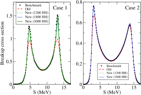
Figure 6: (Color online) Total cross sections (in mb/(MeV sr²)) for the Cases 1 and 2 shown in the upper part of Fig.4 ($E_{in}^{(lab)}=14.1$ MeV). The solid circles are the benchmark calculations in Ref.fri95 . The dashed curves are the results shown in Fig.4, which were computed using the expansion in Eq.(II.3). The cross sections obtained by means of Eq.(II.4) are shown by the dotted, thin-solid, and thick-solid curves, which correspond, respectively, to calculations including 1200, 1800, and 3000 hyperspherical harmonics when computing the integral in Eq.(51).

This is shown in Fig.6, where we show the same cross sections as in Fig.4 for the Cases 1 and 2. The benchmark result is given by the solid circles and the old computed cross sections, as shown in Fig.4, are given by the dashed curves. The cross sections obtained with the new procedure have been computed including 35 adiabatic terms in the expansion in Eq.(51), and the number of hyperspherical harmonics used in the same expansion are 1200 for the dotted curves, 1800 for the thin-solid curves, and 3000 for the thick-solid curve.

Needless to say, when the same procedure is used to compute the cross sections for the Cases 3 and 4, the same results as the ones shown for these two cases in Fig.5 are obtained.

As we can see, in the regions where the results shown in Fig.3 were matching the benchmark, the new calculations still reproduce the results equally well. However, in the peaks where the old calculation and the benchmark did not agree, the new calculation improves the agreement significantly. As already mentioned, the agreement is actually reached when a sufficiently high number of hyperspherical harmonics is included in the calculation. In fact, as we can see, 1200 hyperspherical harmonics are still not enough, and 1800 of them are at least needed in Case 2, and 3000 in Case 1.

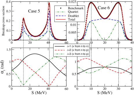
Figure 7: (Color online) Upper part: Total cross sections (in mb/(MeV sr²)) for the Cases 5 and 6 and $E_{in}^{(lab)}=42.0$ MeV (see text). The solid circles are the benchmark calculations in Ref.fri95 . The dot-dashed and dashed curves are the quartet ($J=3/2$) and doublet ($J=1/2$) contributions, respectively. The total cross sections are given by the solid curves. For Case 6 (right panel) the calculation using the expansion in Eq.(II.3) is accurate enough. For Case 5 (left panel) the expansion in Eq.(II.4) is required in order to obtain sufficient accuracy in the vicinity of the peaks. Lower part: For the same two cases, the corresponding values of $\alpha_{i}$ ($i=1,2,3$) as a function of the arclength $S$.

For completeness, we also show the results for the two benchmark calculations given in Ref.fri95 corresponding to an incident energy in the laboratory frame of 42.0 MeV. The angles describing the direction of the outgoing neutrons in these two cases are:

• Case 5: $\theta_{1}=45.0^{\circ}$, $\theta_{2}=60.54^{\circ}$, $\Delta\varphi=180^{\circ}$.

• Case 6: $\theta_{1}=53.61^{\circ}$, $\theta_{2}=53.61^{\circ}$, $\Delta\varphi=120^{\circ}$.

The results for Cases 5 and 6 ($E_{in}^{(lab)}=42.0$ MeV) are shown in Fig.7. As in Figs.4 and 5, the lower part shows the values of the hyperangle $\alpha_{i}$ as a function of the arclength $S$. As we can see, the Case 5 given above is analogous to the Cases 1 and 2 shown in Fig.4, where the hyperangles $\alpha_{2}$ and $\alpha_{3}$ approach zero for certain values of the arclength $S$. Now this happens for values of $S$ around 13 MeV and 40.5 MeV. For this reason, an accurate calculation of the cross section for Case 5 in the vicinity of these two $S$-values requires use of the expansion given in Eq.(II.4). For Case 6 the value of the hyperangle $\alpha$ is always far from zero (as in the Cases 3 and 4 shown in Fig.5), and use of the expansion in Eq.(II.3) is enough to get a sufficient accuracy in the calculations.

The upper part of Fig.7 shows the corresponding cross sections. The dot-dashed and dashed curves are the quartet ($J=3/2$) and doublet ($J=1/2$) contributions, respectively. The total cross section is given by the solid curves. As we can see, the agreement with the benchmark calculations (solid circles) given in Ref.fri95 is very good. In Case 5 the convergence in the vicinity of the two peaks, computed through Eq.(II.4), has required inclusion of up to 40 adiabatic terms in the expansion of the three-body wave function (see Eq.(II.3)). This number is higher than in the calculations for $E_{in}^{(lab)}=14.1$ MeV, where even less than 30 adiabatic channels were enough. This is because for a given value of the hyperradius $\rho$ only the adiabatic potentials whose value at $\rho$ is smaller than the incident energy (or close enough to the energy if they are above) contribute to the radial wave functions $f_{n1}(\rho)$ obtained through Eq.(21). Obviously, the higher the three-body energy $E$ the higher the number of adiabatic potentials contributing to the radial wave functions.

V Summary and conclusions

The description of three-body systems, and in particular of $1+2$ reactions, by use of the adiabatic expansion method has been proved to be efficient provided that the integral relations introduced in Ref.bar09b are used. Because of these two relations the ${\cal S}$-matrix of the reaction can be extracted from the internal part of the wave function, and subsequently the pattern of convergence of the adiabatic expansion is fast. Knowledge of the ${\cal S}$-matrix permits then to obtain accurate results for the total cross sections for the different open channels (elastic, inelastic, transfer, or breakup).

However, even if the ${\cal S}$-matrix and the total cross sections can be accurately computed, it is not obvious that the differential cross sections that one extracts from the ${\cal S}$-matrix are also accurate. In fact, the calculation of the differential cross sections requires knowledge of not only of the ${\cal S}$-matrix, but of the full transition amplitude. When the adiabatic expansion is applied to obtain the transition amplitude, the number of adiabatic terms necessary in order to achieve convergence strongly depends on the geometry of the outgoing particles, and under some circumstances this number can be exceedingly large.

In this work we have given the details of how to compute differential cross sections for 1+2 reactions above the threshold for breakup of the dimer. The expressions that permit to transform the cross sections from the center of mass frame to the laboratory frame have been derived. The three-body wave function describing the three-body system as well as the transition amplitude are computed by use of the adiabatic expansion method.

The case of neutron-deuteron breakup has been taken as a test, and our results have been compared with the benchmark calculations described in Refs.fri95 ; fri90 . Six different geometries have been considered for the three outgoing nucleons after the breakup.

In general, the agreement with the benchmark results has been found to be good. The only discrepancy appears in those cases corresponding to two outgoing particles flying away together after the breakup with zero relative energy. In this case the adiabatic expansion of the transition amplitude is not convenient, since the number of adiabatic terms needed to reproduce such structure is too large.

We have shown that this problem can be solved by skipping the partial wave expansion of the outgoing wave, and expressing the transition amplitude in terms of a full, non-expanded, outgoing plane wave. This calculation is much more demanding from the numerical point of view, and special care has to be taken with the number of hyperspherical harmonics used to describe the incoming wave function.

This study can be seen as a first step in the inclusion of the Coulomb interaction in the study of 1 + 2 nuclear processes. Preliminary studies using the HA expansion have been done in Ref. kie10 for the elastic channel of the $p-d$ reaction. In the breakup case, Eq.(51) can not be applied directly since the free plane wave was used in its derivation, and it should be replaced by a distorted wave due to the long range of the Coulomb potential. This study is at present underway following the analysis given in Ref.viv01 . However, it should be noticed that the configuration in which two protons move away together is suppressed and the one in which a neutron-proton pair moves away together far from the second proton shows tiny Coulomb effects (see Ref.del05 ). Hence, we expect to extend the analysis here presented to the $p-d$ case, and in general to $1+2$ nuclear processes allowing us to analyze several reactions of astrophysical interest in which the inclusion of the Coulomb interaction cannot be avoided.

Appendix A The outgoing flux

The time-dependent Schrödinger equation in hyperspherical coordinates is given by nie01 :

$$i\hbar\frac{\partial\Psi}{\partial t}=\frac{\hbar^{2}}{2m}\left(-\frac{\partial^{2}\Psi}{\partial\rho^{2}}-\frac{5}{\rho}\frac{\partial\Psi}{\partial\rho}\right)+\frac{\hbar^{2}}{2m}\frac{\hat{\Lambda}}{\rho^{2}}\Psi+\hat{V}\Psi,$$ (64)

where $\Psi$ is the three-body wave function, $\hat{\Lambda}$ is the grand-angular operator whose eigenfunctions are the hyperspherical harmonics, and $\hat{V}$ is the operator containing the two-body potentials.

The self-adjoint of the equation above is just:

$$-i\hbar\frac{\partial\Psi^{\dagger}}{\partial t}=\frac{\hbar^{2}}{2m}\left(-\frac{\partial^{2}\Psi^{\dagger}}{\partial\rho^{2}}-\frac{5}{\rho}\frac{\partial\Psi^{\dagger}}{\partial\rho}\right)+\frac{\hbar^{2}}{2m}\Psi^{\dagger}\frac{\hat{\Lambda}}{\rho^{2}}+\Psi^{\dagger}\hat{V},$$ (65)

Multiplying Eq.(64) by $\Psi^{\dagger}$ from the left and Eq.(65) by $\Psi$ from the right we get two expressions that after subtracting lead to:

$$\rho^{5}\frac{\partial|\Psi|^{2}}{\partial t}=-\frac{1}{i}\frac{\hbar}{2m}\frac{\partial}{\partial\rho}\left[\Phi^{\dagger}\frac{\partial\Phi}{\partial\rho}-\frac{\partial\Phi^{\dagger}}{\partial\rho}\Phi\right],$$ (66)

where $\Phi=\rho^{5/2}\Psi$.

Therefore, the number of particles per unit time through the unit of surface of a hypersphere of hyperradius $\rho$ is given by:

$$\frac{1}{i}\frac{\hbar}{2m}\frac{1}{\rho^{5}}\left[\Phi^{\dagger}\frac{\partial\Phi}{\partial\rho}-\frac{\partial\Phi^{\dagger}}{\partial\rho}\Phi\right].$$ (67)

Thus, the flux of particles through an element of hypersurface $d\Sigma$ is given by:

$$\mbox{outgoing flux}=\frac{1}{i}\frac{\hbar}{2m}\frac{1}{\rho^{5}}\left[\Phi^{\dagger}\frac{\partial\Phi}{\partial\rho}-\frac{\partial\Phi^{\dagger}}{\partial\rho}\Phi\right]d\Sigma$$ (68)

The asymptotic behavior of the three-body wave function in hyperspherical coordinates takes the form:

$$\Psi\stackrel{{\scriptstyle\rho\rightarrow\infty}}{{\longrightarrow}}\frac{1}{\rho^{5/2}}e^{i\kappa\rho}A,$$ (69)

where $\kappa=\sqrt{2mE}/\hbar$, $E$ is the total three-body energy, and $A$ is the transition amplitude.

Keeping in mind that $\Phi=\rho^{5/2}\Psi$, substituting Eq.(69) into Eq.(68), and using that the element of hypersurface is given by Eq.(8), we get the following final expression for the outgoing flux:

$$\mbox{outgoing flux}=\hbar\frac{\kappa}{m}|A|^{2}\left(\frac{m}{\mu_{x}}\right)^{3/2}\left(\frac{m}{\mu_{y}}\right)^{3/2}d\Omega_{\kappa},$$ (70)

where we have used that, asymptotically, $d\Omega=d\Omega_{\kappa}$.

Appendix B Phase space for three particles with equal mass.

The choice of three particles with equal mass is made just to simplify the notation and the expressions derived in the following subsections. The mass of the particles $m$ is also taken as the normalization mass in the definition of the Jacobi coordinates given in Eqs.(3) to (6). In any case the extension of the expressions below to particles with different mass is straightforward.

B.1 Center of mass frame

To write down the phase space in the center of mass frame we use the momentum coordinates $\{\bm{p}_{x},\bm{p}_{y},\bm{P}\}$, where $\bm{p}_{x}$ and $\bm{p}_{y}$ are defined in Eqs.(5) and (6), and $\bm{P}=\bm{p}_{i}+\bm{p}_{j}+\bm{p}_{k}$ is the momentum of the three-body center of mass. In these coordinates the phase space takes the form:

$$\Phi=\int d\bm{p}_{x}d\bm{p}_{y}d\bm{P}\delta(E-\frac{\hbar^{2}p_{x}^{2}}{2\mu_{x}}-\frac{\hbar^{2}p_{y}^{2}}{2\mu_{y}})\delta^{(3)}(\bm{P}-\bm{p}_{i}-\bm{p}_{j}-\bm{p}_{k}),$$ (71)

where the delta functions impose energy and momentum conservation ($E$ is the three-body energy in the center of mass frame).

The integration in (71) over $\bm{P}$ can be made trivially thanks to the momentum delta function, and the phase space can be rewritten as:

$$\Phi=\left(\frac{\mu_{x}}{m}\right)^{3/2}\left(\frac{\mu_{y}}{m}\right)^{3/2}\int\kappa^{5}d\kappa d\Omega_{\kappa}\delta\left(E-\frac{\hbar^{2}\kappa^{2}}{2m}\right),$$ (72)

where we have used that according to Eqs.(5) and (6)

$$d\bm{p}_{x}d\bm{p}_{y}=\left(\frac{\mu_{x}}{m}\right)^{3/2}\left(\frac{\mu_{y}}{m}\right)^{3/2}d\bm{k}_{x}d\bm{k}_{y}$$ (73)

and that $d\bm{k}_{x}d\bm{k}_{y}=\kappa^{5}d\kappa d\Omega_{\kappa}$, where $\Omega_{\kappa}$ represents the hyperangles in momentum space.

The delta function in Eq.(72) can be rewritten as:

$$\delta\left(E-\hbar^{2}\frac{\kappa^{2}}{2m}\right)=\frac{m}{\hbar^{2}\kappa}\delta\left(\kappa-\frac{\sqrt{2mE}}{\hbar}\right),$$ (74)

which means that, after integration over $\kappa$, the phase space (72) takes the final form:

$$d^{5}\Phi=\left(\frac{\mu_{x}}{m}\right)^{3/2}\left(\frac{\mu_{y}}{m}\right)^{3/2}\kappa^{4}\frac{m}{\hbar^{2}}d\Omega_{\kappa}.$$ (75)

B.2 Lab frame

Let us consider now the 1+2 reaction in the lab frame, where the momentum of the target (the dimer) is zero, and let us write the phase space $\Phi$ but using the momenta $\bm{p}_{i}$, $\bm{p}_{j}$, and $\bm{p}_{k}$ of the three particles after the breakup. Imposing energy and momentum conservation the phase space takes the form:

$$\Phi = \int d\bm{p}_{i}d\bm{p}_{j}d\bm{p}_{k}\delta\left(E_{lab}-\frac{\hbar^{2}p_{i}^{2}}{2m}-\frac{\hbar^{2}p_{j}^{2}}{2m}-\frac{\hbar^{2}p_{k}^{2}}{2m}\right)$$ (76)

$$\times\delta^{3}(\bm{p}_{y}^{(lab)}-\bm{p}_{i}-\bm{p}_{j}-\bm{p_{k}}),$$

where $\bm{p}_{y}^{(lab)}$ is the momentum of the incoming particle in lab frame, and $E_{lab}$ is the total three-body energy in the lab frame:

$$E_{lab}=E_{in}^{(lab)}+E_{d}=\frac{\hbar^{2}p_{y}^{(lab)2}}{2m}+E_{d},$$ (77)

where $E_{in}^{(lab)}$ is the energy of the projectile in the lab frame and $E_{d}$ is the binding energy of the dimer ($E_{d}<0$). For the particular case of three particles with equal mass, the incident momentum in the lab frame is related to the one in the center of mass frame, $\bm{p}_{y}$, by the simple relation $\bm{p}_{y}^{(lab)}=3\bm{p}_{y}/2$.

Making use of the momentum delta function we integrate now over $\bm{p}_{k}$, which leads to:

$$\Phi=\int d\bm{p}_{i}d\bm{p}_{j}\delta\left(f(\bm{p}_{i},\bm{p}_{j})\right)$$ (78)

where

$$f(\bm{p}_{i},\bm{p}_{j})=E_{lab}-\frac{\hbar^{2}p_{i}^{2}}{2m}-\frac{\hbar^{2}p_{j}^{2}}{2m}-\frac{\hbar^{2}(\bm{p}_{y}^{(lab)}-\bm{p}_{i}-\bm{p}_{j})^{2}}{2m}$$ (79)

Using Eq.(77) the function above can be written as:

$$f(\bm{p}_{i},\bm{p}_{j}) = E_{d}-\frac{\hbar^{2}p_{i}^{2}}{m}-\frac{\hbar^{2}p_{j}^{2}}{m}+$$

$$+\frac{\hbar^{2}}{m}\left(p_{y}^{(lab)}p_{i}\mu_{i}+p_{y}^{(lab)}p_{j}\mu_{j}-p_{i}p_{j}\mu\right)$$

with

$$\mu_{i} = \frac{\bm{p}_{y}^{(lab)}\cdot\bm{p}_{i}}{p_{y}^{(lab)}p_{i}}=\cos{\theta_{p_{i}}}$$ (81)

$$\mu_{j} = \frac{\bm{p}_{y}^{(lab)}\cdot\bm{p}_{j}}{p_{y}^{(lab)}p_{j}}=\cos{\theta_{p_{j}}}$$ (82)

$$\mu = \frac{\bm{p}_{i}\cdot\bm{p}_{j}}{p_{i}p_{j}}=\sin{\theta_{p_{i}}}\sin{\theta_{p_{j}}}\cos\Delta\varphi+\mu_{i}\mu_{j},$$ (83)

where $\theta_{p_{i}}$ and $\theta_{p_{j}}$ are the polar angles associated to the direction of $\bm{p}_{i}$ and $\bm{p}_{j}$, respectively, and $\Delta\varphi$ is the difference between the corresponding azimuthal angles. The $z$-axis is chosen along the momentum $\bm{p}_{y}^{(lab)}$.

We shall now exploit the well known property of the delta function:

$$\delta(g(x))=\sum_{i}\frac{1}{|g^{\prime}(x_{i})|}\delta(x-x_{i})$$ (84)

where the summation is over all the $x_{i}$ values satisfying $g(x_{i})=0$, and where $g^{\prime}(x_{i})$ is the value of the first derivative of $g(x)$ at the point $x_{i}$. Getting thus the derivative of Eq.(B.2) with respect to $p_{i}$, and using Eq.(84), it is then easy to rewrite $\delta(f(\bm{p}_{i},\bm{p}_{j}))$ in a more convenient form and integrate Eq.(78) over $p_{i}$, which leads to:

$$\Phi=\frac{m}{\hbar^{2}}\int p_{j}^{2}dp_{j}d\hat{\bm{p}}_{i}d\hat{\bm{p}}_{j}\frac{p_{i}^{2}}{|2p_{i}-p_{y}^{(lab)}\mu_{i}+p_{j}\mu|},$$ (85)

where for each value of $p_{j}$ and the directions $\hat{\bm{p}}_{i}$ and $\hat{\bm{p}}_{j}$, $p_{i}$ is obtained as the solution of

$$E_{d}-\frac{\hbar^{2}p_{i}^{2}}{m}-\frac{\hbar^{2}p_{j}^{2}}{m}+$$ (86)

$$+\frac{\hbar^{2}}{m}\left(p_{y}^{(lab)}p_{i}\mu_{i}+p_{y}^{(lab)}p_{j}\mu_{j}-p_{i}p_{j}\mu\right)=0.$$

In the same way it is possible to integrate Eq.(78) over $p_{j}$ instead of $p_{i}$, and get:

$$\Phi=\frac{m}{\hbar^{2}}\int p_{i}^{2}dp_{i}d\hat{\bm{p}}_{i}d\hat{\bm{p}}_{j}\frac{p_{j}^{2}}{|2p_{j}-p_{y}^{(lab)}\mu_{j}+p_{i}\mu|}.$$ (87)

From Eqs.(85) and (87) it is then clear that:

$$\frac{dp_{j}}{|2p_{i}-p_{y}^{(lab)}\mu_{i}+p_{j}\mu|}=\frac{dp_{i}}{|2p_{j}-p_{y}^{(lab)}\mu_{j}+p_{i}\mu|}$$ (88)

Since the energy $E_{i}$ of particle $i$ is given by $E_{i}=\hbar^{2}p_{i}^{2}/2m$ we have that $dE_{i}=\hbar^{2}p_{i}dp_{i}/m$ (and the same for particle $j$), and the expression above can be written as:

$$\frac{p_{i}dE_{j}}{|2p_{i}-p_{y}^{(lab)}\mu_{i}+p_{j}\mu|}=\frac{p_{j}dE_{i}}{|2p_{j}-p_{y}^{(lab)}\mu_{j}+p_{i}\mu|},$$ (89)

or, in other words:

$$dE_{j}=\frac{p_{j}|2p_{i}-p_{y}^{(lab)}\mu_{i}+p_{j}\mu|}{p_{i}|2p_{j}-p_{y}^{(lab)}\mu_{j}+p_{i}\mu|}dE_{i}.$$ (90)

We now define the arclength $S$ such that:

$$dS=\sqrt{(dE_{i})^{2}+(dE_{j})^{2}},$$ (91)

which from Eq.(90) leads to:

$$dE_{i}=$$

$$\frac{p_{i}|2p_{j}-p_{y}^{(lab)}\mu_{j}+p_{i}\mu|dS}{\left[p_{i}^{2}(2p_{j}-p_{y}^{(lab)}\mu_{j}+p_{i}\mu)^{2}+p_{j}^{2}(2p_{i}-p_{y}^{(lab)}\mu_{i}+p_{j}\mu)^{2}\right]^{1/2}}$$

Finally, keeping in mind that $E_{i}=\hbar^{2}p_{i}^{2}/2m$ and therefore $p_{i}dp_{i}=(m/\hbar^{2})dE_{i}$, we can write the phase space Eq.(87) as:

$$\Phi=\left(\frac{m}{\hbar^{2}}\right)^{2}\int p_{i}dE_{i}d\hat{\bm{p}}_{i}d\hat{\bm{p}}_{j}\frac{p_{j}^{2}}{|2p_{j}-p_{y}^{(lab)}\mu_{j}+p_{i}\mu|},$$ (93)

which by use of Eq.(B.2) leads to the final expression for the phase space in the lab frame:

$$d^{5}\Phi=\left(\frac{m}{\hbar^{2}}\right)^{2}K_{S}dSd\hat{\bm{p}}_{i}d\hat{\bm{p}}_{j},$$ (94)

where

$$K_{S}=$$

$$\frac{p_{i}^{2}p_{j}^{2}}{\left[p_{i}^{2}(2p_{j}-p_{y}^{(lab)}\mu_{j}+p_{i}\mu)^{2}+p_{j}^{2}(2p_{i}-p_{y}^{(lab)}\mu_{i}+p_{j}\mu)^{2}\right]^{1/2}}$$

Appendix C Calculation of $p_{i}$ and $p_{j}$ for a given input

In this work the $n-d$ breakup reaction is investigated taking as input the incident energy of the projectile in the lab frame $E_{in}^{(lab)}$, the polar angles $\theta_{p_{i}}$ and $\theta_{p_{j}}$ of the two neutrons observed after the breakup, and the difference between the corresponding two azimuthal angles $\Delta\varphi$.

From the energy $E_{in}^{(lab)}$ we can easily obtain the incident momentum of the projectile in the lab frame ($p_{y}^{(lab)}$), the incident momentum in the center of mass frame ($p_{y}^{(in)}$) and the three-body momentum $\kappa$ (see Eq.(16) and below).

The angles $\theta_{p_{i}}$, $\theta_{p_{j}}$, and $\Delta\varphi$ permit us to obtain $\mu_{i}$, $\mu_{j}$, and $\mu$, which are given by Eqs.(81), (82), and (83), respectively.

The remaining point is to determine for each value of the arclength $S$ the values of $p_{i}$ and $p_{j}$, such that we can obtain $K_{S}$ according to Eq.(B.2), and then obtain the cross section (15) as a function of $S$.

The momenta $p_{i}$ and $p_{j}$ are not independent. They are related through the expression (86), which can be written as:

$$\alpha^{2}+p_{i}^{2}+p_{j}^{2}-p_{y}^{(lab)}p_{i}\mu_{i}-p_{y}^{(lab)}p_{j}\mu_{j}+p_{i}p_{j}\mu=0,$$ (96)

where $\alpha^{2}=-mE_{d}/\hbar^{2}$ ($E_{d}<0$).

After some algebra the equation above can be seen to describe an ellipse, whose equation is given by:

$$\frac{(p^{\prime}_{i}-p^{C}_{i})^{2}}{a_{i}^{2}}+\frac{(p^{\prime}_{j}-p_{j}^{C})^{2}}{a_{j}^{2}}=1,$$ (97)

where

$$p^{C}_{i} = \frac{p_{y}^{(lab)}}{2\sqrt{2}}\frac{\mu_{i}-\mu_{j}}{1-\mu/2}$$ (98)

$$p^{C}_{j} = \frac{p_{y}^{(lab)}}{2\sqrt{2}}\frac{\mu_{i}+\mu_{j}}{1+\mu/2},$$ (99)

and $a_{i}$ and $a_{j}$ are given as

$$a_{i} = \frac{\beta}{\sqrt{1-\frac{\mu}{2}}},$$ (100)

$$a_{j} = \frac{\beta}{\sqrt{1+\frac{\mu}{2}}},$$ (101)

with

$$\beta^{2}=\frac{p_{y}^{(lab)2}}{8}\left[\frac{(\mu_{i}-\mu_{j})^{2}}{1-\frac{\mu}{2}}+\frac{(\mu_{i}+\mu_{j})^{2}}{1+\frac{\mu}{2}}\right]-\alpha^{2}$$ (102)

Note that given the input, $p_{i}^{C}$, $p_{j}^{C}$, $a_{i}$, and $a_{j}$ are just numbers.

Finally, $p^{\prime}_{i}$ and $p^{\prime}_{j}$ are such that:

$$p_{i} = \frac{p^{\prime}_{i}+p^{\prime}_{j}}{\sqrt{2}},$$ (103)

$$p_{j} = \frac{p^{\prime}_{j}-p^{\prime}_{i}}{\sqrt{2}}.$$ (104)

The equation of the ellipse (97) can be written in parametric form as:

$$p^{\prime}_{i}-p_{i}^{C} = a_{i}\cos{\tilde{\varphi}},$$ (105)

$$p^{\prime}_{j}-p_{j}^{C} = a_{j}\sin{\tilde{\varphi}},$$ (106)

which permit to write Eqs.(103) and (104) as:

$$p_{i} = \frac{a_{i}\cos{\tilde{\varphi}}+p_{i}^{C}+a_{j}\sin{\tilde{\varphi}}+p_{j}^{C}}{\sqrt{2}},$$ (107)

$$p_{j} = \frac{a_{j}\sin{\tilde{\varphi}}+p_{j}^{C}-a_{i}\cos{\tilde{\varphi}}-p_{i}^{C}}{\sqrt{2}},$$ (108)

from which we get:

$$dp_{i} = \frac{-a_{i}\sin{\tilde{\varphi}}+a_{j}\cos{\tilde{\varphi}}}{\sqrt{2}}d\tilde{\varphi},$$ (109)

$$dp_{j} = \frac{a_{j}\cos{\tilde{\varphi}}+a_{i}\sin{\tilde{\varphi}}}{\sqrt{2}}d\tilde{\varphi}.$$ (110)

Reminding now that $dE_{i}=\hbar^{2}p_{i}dp_{i}/m$, and making use of the two equations above, we can write the arclength $S$ given in Eq.(91) as:

$$dS=F(\tilde{\varphi})d\tilde{\varphi},$$ (111)

where

$$F(\tilde{\varphi})=$$

$$\frac{\hbar^{2}}{m}\frac{1}{\sqrt{2}}\left[p_{i}^{2}(a_{j}\cos{\tilde{\varphi}}-a_{i}\sin{\tilde{\varphi}})^{2}+p_{j}^{2}(a_{j}\cos{\tilde{\varphi}}+a_{i}\sin{\tilde{\varphi}})^{2}\right]^{1/2},$$

where $p_{i}$ and $p_{j}$ are given as a function of $\tilde{\varphi}$ by Eqs.(107) and (108), respectively.

Therefore, the arclength $S$ can be obtained as a function of $\tilde{\varphi}$ from the expression:

$$S(\tilde{\varphi})=\int_{\tilde{\varphi}_{0}}^{\tilde{\varphi}}F(\tilde{\varphi}^{\prime})d\tilde{\varphi}^{\prime},$$ (113)

where, for all the cases except case 3, $\tilde{\varphi}_{0}$ is defined such that for $\tilde{\varphi}=\tilde{\varphi}_{0}$ then $p_{j}=0$. For case 3, since the ellipse in Eq.(97) does not cross the $p_{j}=0$ axis, $\tilde{\varphi}_{0}$ is defined such that for $\tilde{\varphi}=\tilde{\varphi}_{0}$ then $p_{i}=0$.

In a practical case, given a value of $S$, one has to determine the angle $\tilde{\varphi}$ such that $S(\tilde{\varphi})=S$. With this value of $\tilde{\varphi}$ the values of $p_{i}$ and $p_{j}$ are immediately obtained from Eqs.(107) and (108).

Appendix D Adiabatic expansion of three-body continuum wave functions

In the appendix of Ref.dan04 the authors give the general solution of the coupled-channel problem for three-body continuum states in the presence of interaction potentials. Keeping the notation used in that reference, the continuum three-body wave function at a given three-body energy $E=\kappa^{2}\hbar^{2}/2m$ is written as:

$$\Psi = \sum_{JM}\frac{(2\pi)^{3}}{(\kappa\rho)^{5/2}}\sum_{K\gamma,K^{\prime}\gamma^{\prime}}\psi^{J}_{K\gamma,K^{\prime}\gamma^{\prime}}(\kappa\rho)\Upsilon_{JM}^{K\gamma}(\Omega_{\rho})$$ (114)

$$\times\sum_{M^{\prime}_{L}M^{\prime}_{S}}\langle L^{\prime}M^{\prime}_{L}S^{\prime}M^{\prime}_{S}|JM\rangle{\cal Y}_{K^{\prime}L^{\prime}M^{\prime}_{L}}^{\ell^{\prime}_{x}\ell^{\prime}_{y}}(\Omega_{\kappa})^{*},$$

where the functions ${\cal Y}_{K^{\prime}L^{\prime}M^{\prime}_{L}}^{\ell^{\prime}_{x}\ell^{\prime}_{y}}$ are the usual hyperspherical harmonics, the index $\gamma$ collects the quantum numbers $\{\ell_{x},\ell_{y},L,S\}$, and $\Upsilon_{JM}^{K\gamma}$ is defined as the coupling between the hyperspherical harmonic ${\cal Y}_{KLM_{L}}^{\ell_{x}\ell_{y}}$ and the three-body spin function $\chi_{SM_{S}}$:

$$\Upsilon_{JM}^{K\gamma}(\Omega_{\rho})=\sum_{M_{L}M_{S}}\langle LM_{L}SM_{S}|JM\rangle{\cal Y}_{KLM_{L}}^{\ell_{x}\ell_{y}}(\Omega_{\rho})\chi_{SM_{S}}.$$ (115)

It is convenient to write the total three-body wave function as $\Psi=\sum_{S^{\prime}M^{\prime}_{S}}\Psi_{S^{\prime}M^{\prime}_{S}}$, where:

$$\Psi_{S^{\prime}M^{\prime}_{S}} = \sum_{JM}\frac{(2\pi)^{3}}{(\kappa\rho)^{5/2}}\sum_{K\gamma}\sum_{K^{\prime}\ell^{\prime}_{x}\ell^{\prime}_{y}L^{\prime}}\psi^{J}_{K\gamma,K^{\prime}\gamma^{\prime}}(\kappa\rho)\Upsilon_{JM}^{K\gamma}(\Omega_{\rho})$$ (116)

$$\times\sum_{M^{\prime}_{L}}\langle L^{\prime}M^{\prime}_{L}S^{\prime}M^{\prime}_{S}|JM\rangle{\cal Y}_{K^{\prime}L^{\prime}M^{\prime}_{L}}^{\ell^{\prime}_{x}\ell^{\prime}_{y}}(\Omega_{\kappa})^{*},$$

which represents the continuum three-body wave function where the spin function of the incoming channel is described by the quantum numbers $S^{\prime}$ and $M^{\prime}_{S}$.

This can be easily seen because in the case of no interaction between the particles, the radial wave functions $\psi^{J}_{K\gamma,K^{\prime}\gamma^{\prime}}(\kappa\rho)$ reduce to $i^{K}\sqrt{\kappa\rho}J_{K+2}(\kappa\rho)\delta_{KK^{\prime}}\delta_{\gamma,\gamma^{\prime}}$, and the three-body wave function becomes:

$$\Psi_{S^{\prime}M^{\prime}_{S}}\stackrel{{\scriptstyle\mbox{\tiny no interaction}}}{{\longrightarrow}}e^{i(\bm{k}_{x}\cdot\bm{x}+\bm{k}_{y}\cdot\bm{y})}\chi_{S^{\prime}M^{\prime}_{S}},$$ (117)

which is a three-body plane wave multiplied by the three-body spin function in the incoming channel.

Using now the expression Eq.(115) the wave function in Eq.(116) can be written in a more compact way as:

$$\Psi_{S^{\prime}M^{\prime}_{S}} = \sum_{JM}\frac{(2\pi)^{3}}{(\kappa\rho)^{5/2}}\sum_{K\gamma}\sum_{K^{\prime}\ell^{\prime}_{x}\ell^{\prime}_{y}L^{\prime}}\psi^{J}_{K\gamma,K^{\prime}\gamma^{\prime}}(\kappa\rho)\Upsilon_{JM}^{K\gamma}(\Omega_{\rho})$$ (118)

$$\times\langle\chi_{S^{\prime}M^{\prime}_{S}}|\Upsilon_{JM}^{K^{\prime}\gamma^{\prime}}(\Omega_{\kappa})\rangle^{*}.$$

The transformation of the wave function $\Psi_{S^{\prime}M^{\prime}_{S}}$ from the HH basis to the basis formed by the hyperangular functions $\Phi^{JM}_{n}$ defined in Eq.(19) can be easily made through the relation

$$\Upsilon_{JM}^{K\gamma}=\sum_{n}\langle\Phi^{JM}_{n}|\Upsilon_{JM}^{K\gamma}\rangle\Phi^{JM}_{n},$$ (119)

which leads to:

$$\Psi_{S^{\prime}M^{\prime}_{S}} = \sum_{JM}\frac{(2\pi)^{3}}{(\kappa\rho)^{5/2}}$$

$$\times\sum_{nn^{\prime}}f_{nn^{\prime}}^{S^{\prime}J}(\kappa\rho)\Phi^{JM}_{n}(\rho,\Omega_{\rho})\langle\chi_{S^{\prime}M^{\prime}_{S}}|\Phi^{JM}_{n^{\prime}}(\kappa,\Omega_{\kappa})\rangle^{*},$$

and where we have defined:

$$f_{nn^{\prime}}^{S^{\prime}J}(\kappa\rho)=$$ (121)

$$\sum_{K\gamma}\sum_{K^{\prime}\ell^{\prime}_{x}\ell^{\prime}_{y}L^{\prime}}\psi^{J}_{K\gamma,K^{\prime}\gamma^{\prime}}(\kappa\rho)\langle\Phi^{JM}_{n}(\rho,\Omega_{\rho})|\Upsilon_{JM}^{K\gamma}(\Omega_{\rho})\rangle$$

$$\langle\Upsilon_{JM}^{K^{\prime}\gamma^{\prime}}(\Omega_{\kappa})|\Phi^{JM}_{n^{\prime}}(\kappa,\Omega_{\kappa})\rangle.$$

As shown in Eq.(117), the expansion in Eq.(114) has been written in such a way that in case of no interaction between the particles the wave function Eq.(116) reduces basically to a three-body plane. In fact, the way they are written, Eqs.(114) or (116) are appropriate to describe $3\rightarrow 3$ reactions, and would permit to extract the corresponding $3\rightarrow 3$ transition amplitude.

However, when dealing with 1+2 reactions, in case of no interaction between the projectile and the dimer, the three-body continuum wave function must reduce to

$$\Psi_{\sigma_{d}\sigma_{p}}\stackrel{{\scriptstyle\mbox{\tiny no interaction}}}{{\longrightarrow}}e^{i\bm{k}_{y}\cdot\bm{y}}\chi_{s_{d}\sigma_{d}}\chi_{s_{p}\sigma_{p}},$$ (122)

where $\chi_{s_{d}\sigma_{d}}$ is the dimer wave function (with spin $s_{d}$ and projection $\sigma_{d}$), and $\chi_{s_{p}\sigma_{p}}$ is the spin function of the projectile. As we can see, the three-body plane wave is now an ordinary two-body plane wave (describing the relative free motion between the projectile and the dimer center of mass). In order to obtain such two-body plane wave with the correct normalization the factor $(2\pi)^{3}$ in the expansion in Eq.(114), and therefore also in the following expressions of the continuum wave function, has to be replaced by $(2\pi)^{3/2}$.

Also, as seen from Eq.(122), if we want to describe the incoming spin state by $\chi_{s_{d}\sigma_{d}}\chi_{s_{p}\sigma_{p}}$ (instead of the total three-body spin and projection $S^{\prime}$ and $M^{\prime}_{S}$), the corresponding wave function $\Psi_{\sigma_{d}\sigma_{p}}$ can be obtained from $\Psi_{S^{\prime}M^{\prime}_{S}}$ through the simple relation:

$$\Psi_{\sigma_{d}\sigma_{p}}=\sum_{S^{\prime}M^{\prime}_{S}}\langle\chi_{S^{\prime}M^{\prime}_{S}}|\sigma_{p}\sigma_{d}\rangle\Psi_{S^{\prime}M^{\prime}_{S}},$$ (123)

where $|\sigma_{p}\sigma_{d}\rangle$ represents the spin state $|\chi_{s_{d}\sigma_{d}}\chi_{s_{p}\sigma_{p}}\rangle$, and from which we can write:

$$\Psi_{\sigma_{d}\sigma_{p}}=$$

$$\sum_{JM}\frac{(2\pi)^{3/2}}{(\kappa\rho)^{5/2}}\sum_{nn^{\prime}}f_{nn^{\prime}}^{J}(\kappa\rho)\Phi^{JM}_{n}(\rho,\Omega_{\rho})\langle\sigma_{d}\sigma_{p}|\Phi^{JM}_{n^{\prime}}(\kappa,\Omega_{\kappa})\rangle^{*},$$

where

$$f_{nn^{\prime}}^{J}(\kappa\rho)=\sum_{S^{\prime}M^{\prime}_{S}}\langle\chi_{S^{\prime}M^{\prime}_{S}}|\sigma_{d}\sigma_{p}\rangle f_{nn^{\prime}}^{S^{\prime}J}(\kappa\rho)\langle\sigma_{d}\sigma_{p}|\chi_{S^{\prime}M^{\prime}_{S}}\rangle,$$ (125)

and where we have assumed that the final radial wave functions do not depend on the spin projections, and that the interaction does not mix different spin states $|\sigma_{d}\sigma_{p}\rangle$.

As usual, in Eq.(D) the indices $n$ and $n^{\prime}$ refer to the outgoing and incoming channels, respectively, and Eq.(D) gives the full three-body wave function, where all the possible incoming and outgoing channels are contained. Only the spin projection in the incoming channel are specified. If we now consider a specific incoming channel, let us say channel 1, the summation over $n^{\prime}$ disappears, and $n^{\prime}=1$. Also, if we want to restrict ourselves to outgoing breakup channels, the summation over $n$ should run only over the adiabatic terms associated to breakup of the dimer. In particular, for the case in which only one 1+2 channel exist (the incoming channel 1), we have that the summation over $n$ runs over all $n>1$.

Finally, if we project over a specific spin state $|\sigma_{i}\sigma_{j}\sigma_{k}\rangle$ for the three particles after the breakup, we then get the final expression for the adiabatic expansion of the three-body wave function describing the breakup of the dimer, and it is given by:

$$\Psi_{\sigma_{d}\sigma_{p}}^{\sigma_{i}\sigma_{j}\sigma_{k}} = \sum_{JM}\frac{(2\pi)^{3/2}}{(\kappa\rho)^{5/2}}\sum_{n>1}f_{n1}^{J}(\kappa\rho)$$

$$\langle\sigma_{i}\sigma_{j}\sigma_{k}|\Phi^{JM}_{n}(\rho,\Omega_{\rho})\rangle\langle\sigma_{d}\sigma_{p}|\Phi^{JM}_{n^{\prime}}(\kappa,\Omega_{\kappa})\rangle^{*}.$$

Appendix E Asymptotic incoming angular eigenfunction in momentum space

In coordinate space, the angular eigenfunction $\Phi_{1}(\rho,\Omega_{\rho})$ associated to a 1+2 channel behaves for large values of $\rho$ as nie01 :

$$\Phi_{1}^{JM}(\rho,\Omega_{\rho})\stackrel{{\scriptstyle\rho\rightarrow\infty}}{{\rightarrow}}$$

$$\left(\frac{m}{\mu_{x}}\right)^{3/4}\rho^{3/2}\left[\psi_{d}^{j_{x}}(\bm{r}_{x})\otimes\left[Y_{\ell_{y}}(\Omega_{y})\otimes\chi_{s_{y}}\right]^{j_{y}}\right]^{JM},$$

where $\psi_{d}^{j_{x}}(\bm{r}_{x})$ is the dimer wave function, which is normalized to 1 in the relative coordinate $\bm{r}_{x}$ between the two particles in the dimer, and whose angular momentum is denoted by $j_{x}$. The projectile-dimer relative orbital angular momentum, $\ell_{y}$, and the spin of the projectile, $s_{y}$, couple to the total angular momentum $j_{y}$, which in turn couples to $j_{x}$ to provide the total angular momentum $J$ of the three-body system, whose projection is given by $M$. Finally, $\mu_{x}$ is the reduced mass of the two particles in the dimer.

After a Fourier transformation the dimer wave function becomes $\psi_{d}^{j_{x}}(\bm{p}_{x})$, also normalized to 1 in $\bm{p}_{x}$, where $\bm{p}_{x}$ is the relative momentum between the two particles in the dimer (Eq.(5)). Also, the polar and azimuthal angles $\Omega_{y}$ describing the direction of the Jacobi coordinate $\bm{y}$ become $\Omega_{k_{y}}$, which describe the direction of the incident Jacobi momentum $\bm{k}_{y}^{(in)}$ defined as in Eq.(6). Therefore, the Fourier transform of Eq.(E) must have the form:

$$\Phi_{1}^{JM}(\kappa,\Omega_{\kappa})\rightarrow C\left[\psi_{d}^{j_{x}}(\bm{p}_{x})\otimes\left[Y_{\ell_{y}}(\Omega_{k_{y}})\otimes\chi_{s_{y}}\right]^{j_{y}}\right]^{JM},$$ (128)

where $C$ is a normalization constant.

The value of $C$ can be obtained by imposing that:

$$\int d\Omega_{\kappa}\left|\Phi_{1}(\kappa,\Omega_{\kappa})\right|^{2}=1,$$ (129)

which after using the expansion

$$\Psi_{d}^{j_{x}m_{x}}(\bm{p}_{x})=\sum_{\ell_{x}s_{x}}\Psi^{j_{x}}_{\ell_{x}s_{x}}(p_{x})\left[Y_{\ell_{x}}(\Omega_{k_{x}})\otimes\chi_{s_{x}}\right]^{j_{x}m_{x}}$$ (130)

leads to:

$$\left|C\right|^{2}\int d\alpha_{\kappa}\sin^{2}\alpha_{\kappa}\cos^{2}\alpha_{\kappa}\sum_{\ell_{x}s_{x}}\left|\Psi^{j_{x}}_{\ell_{x}s_{x}}(p_{x})\right|^{2}=1.$$ (131)

Using now that $k_{x}=\kappa\sin\alpha_{\kappa}$ (and therefore $dk_{x}=\kappa\cos\alpha_{\kappa}d\alpha_{\kappa}$) and $k_{y}^{(in)}=\kappa\cos\alpha_{\kappa}$, the expression above can be rewritten as:

$$\left|C\right|^{2}\frac{k_{y}^{(in)}}{\kappa^{4}}\int dk_{x}k_{x}^{2}\sum_{\ell_{x}s_{x}}\left|\Psi^{j_{x}}_{\ell_{x}s_{x}}(p_{x})\right|^{2}=1,$$ (132)

which, after taking into account that $k_{x}^{2}dk_{x}=(m/\mu_{x})^{3/2}p_{x}^{2}dp_{x}$, and keeping in mind that $\psi_{d}^{j_{x}}(\bm{p}_{x})$ is normalized to 1 in $\bm{p}_{x}$, leads to:

$$\left|C\right|^{2}=\frac{\kappa^{4}}{k_{y}^{(in)}}\left(\frac{\mu_{x}}{m}\right)^{3/2},$$ (133)

and therefore:

$$\Phi_{1}^{JM}(\kappa,\Omega_{\kappa})\rightarrow$$

$$\frac{\kappa^{2}}{\sqrt{k_{y}^{(in)}}}\left(\frac{\mu_{x}}{m}\right)^{3/4}\left[\psi_{d}^{j_{x}}(\bm{p}_{x})\otimes\left[Y_{\ell_{y}}(\Omega_{k_{y}})\otimes\chi_{s_{y}}\right]^{j_{y}}\right]^{JM}.$$

In the particular case of only relative $s$-waves between the particles, the expression above reduces to:

$$\Phi_{1}^{JM}(\kappa,\Omega_{\kappa})\rightarrow$$

$$\frac{1}{\sqrt{4\pi}}\left(\frac{\mu_{x}}{m}\right)^{3/4}\frac{\kappa^{2}}{\sqrt{k_{y}^{(in)}}}\left[\psi_{d}^{s_{d}}(\bm{p}_{x})\otimes\chi_{s_{p}}\right]^{JM},$$

where we have recovered the notation of Section II.3, where $s_{d}$ represents the spin of the dimer and $s_{p}$ is the spin of the projectile.

From Eq.(E) it is now simple to see that the projection over the intrinsic states of projectile and target, the asymptotic incoming angular wave function in momentum space is given by:

$$\langle\sigma_{d}\sigma_{p}|\Phi_{1}^{*}(\kappa,\Omega_{\kappa})\rangle=\frac{1}{\sqrt{4\pi}}\left(\frac{\mu_{x}}{m}\right)^{3/4}\frac{\kappa^{2}}{\sqrt{k_{y}^{(in)}}}\langle s_{d}\sigma_{d}s_{p}\sigma_{p}|JM\rangle,$$ (136)

which is the expression given in Eq.(25).

Appendix F Fresnel integrals

The aim of this section is to compute analytically the integral:

$$\int_{y_{\mbox{\scriptsize max}}}^{\infty}dy\left(\frac{C_{m}\sin(\kappa y)\sin(k_{y}y)}{y^{m+3/2}}+\frac{D_{m}\cos(\kappa y)\sin(k_{y}y)}{y^{m+3/2}}\right),$$ (137)

which can also be written as:

$$\frac{C_{m}}{2}\int_{y_{\mbox{\scriptsize max}}}^{\infty}dy\frac{\cos((\kappa-k_{y})y)-\cos((\kappa+k_{y})y)}{y^{m+3/2}}-$$

$$\frac{D_{m}}{2}\int_{y_{\mbox{\scriptsize max}}}^{\infty}dy\frac{\sin((\kappa-k_{y})y)-\sin((\kappa+k_{y})y)}{y^{m+3/2}}.$$

Therefore, the calculation of the integrals above requires just the calculation of the integrals of the type:

$$\int_{y_{\mbox{\scriptsize max}}}^{\infty}dy\frac{\cos(ay)}{y^{m+3/2}}\mbox{ and }\int_{y_{\mbox{\scriptsize max}}}^{\infty}dy\frac{\sin(ay)}{y^{m+3/2}},$$ (139)

where $a$ can be either $(\kappa-k_{y})$ or $(\kappa+k_{y})$.

Taking now $t=ay$ the two integrals above take the form:

$$a^{m+1/2}\int_{t_{\mbox{\scriptsize max}}}^{\infty}dt\frac{\cos t}{t^{m+3/2}}\mbox{ and }a^{m+1/2}\int_{t_{\mbox{\scriptsize max}}}^{\infty}dt\frac{\sin t}{t^{m+3/2}},$$ (140)

where $t_{\mbox{\scriptsize max}}=ay_{\mbox{\scriptsize max}}$.

Let us now define:

$$\tilde{S}_{\nu}(z) = \int_{z}^{\infty}dx\frac{\sin x}{x^{\nu}}$$ (141)

$$\tilde{C}_{\nu}(z) = \int_{z}^{\infty}dx\frac{\cos x}{x^{\nu}},$$ (142)

such that the two integrals in Eq.(140) are $\tilde{C}_{3/2}(t_{\mbox{\scriptsize max}})$ and $\tilde{S}_{3/2}(t_{\mbox{\scriptsize max}})$, respectively.

If we now take into account that:

$$\frac{\sin x}{x^{\nu}}dx = \frac{1}{\nu-1}\frac{\cos x}{x^{\nu-1}}dx-\frac{1}{\nu-1}d\left(\frac{\sin x}{x^{\nu-1}}\right)$$ (143)

$$\frac{\cos x}{x^{\nu}}dx = -\frac{1}{\nu-1}\frac{\sin x}{x^{\nu-1}}dx-\frac{1}{\nu-1}d\left(\frac{\cos x}{x^{\nu-1}}\right),$$ (144)

we can the immediately get the recurrence relations:

$$\tilde{S}_{\nu}(z) = \frac{1}{\nu-1}\frac{\sin z}{z^{\nu-1}}+\frac{1}{\nu-1}\tilde{C}_{\nu-1}(z)$$ (145)

$$\tilde{C}_{\nu}(z) = \frac{1}{\nu-1}\frac{\cos z}{z^{\nu-1}}-\frac{1}{\nu-1}\tilde{S}_{\nu-1}(z),$$ (146)

Therefore, knowledge of $\tilde{S}_{1/2}(z)$ and $\tilde{C}_{1/2}(z)$ would permit, through the recurrence relations in Eqs.(145) and (146) to obtain the integrals in Eq.(139), and therefore the integral in Eq.(F) (or (137)).

The integrals $\tilde{S}_{1/2}(z)$ and $\tilde{C}_{1/2}(z)$ are known analytically, and they are given by:

$$\tilde{S}_{1/2}(z) = \sqrt{\frac{\pi}{2}}-\frac{\sqrt{\pi}}{2}\left(\sqrt{i}\mbox{ erf}(\sqrt{iz})+\sqrt{-i}\mbox{ erf}(\sqrt{-iz})\right)$$

$$\tilde{C}_{1/2}(z) = \sqrt{\frac{\pi}{2}}-\frac{\sqrt{\pi}}{2}\left(\sqrt{-i}\mbox{ erf}(\sqrt{-iz})+\sqrt{i}\mbox{ erf}(\sqrt{iz})\right),$$

where “erf” stands for the usual error function.

References

- (1) E. Nielsen, D.V. Fedorov, A.S. Jensen, and E. Garrido, Phys. Rep. 347, 373 (2001).
- (2) P. Barletta and A. Kievsky, Few-Body Syst. 45, 25 (2009).
- (3) P. Barletta, C. Romero-Redondo, A. Kievsky, M. Viviani, E. Garrido, Phys. Rev. Lett 103, 090402 (2009).
- (4) C. Romero-Redondo, E.Garrido, P. Barletta, A. Kievsky, M. Viviani, Phys. Rev. A 83, 022705 (2011).
- (5) A. Kievsky, M. Viviani, P. Barletta, C. Romero-Redondo, E. Garrido, Phys. Rev. C 81, 034002 (2010).
- (6) E. Garrido, C. Romero-Redondo, A. Kievsky, M. Viviani, Phys. Rev. A 86, 052709 (2012).
- (7) E. Garrido, M. Gattobigio, and A. Kievsky, Phys. Rev. A 88, 032701 (2013).
- (8) G.L. Payne, W. Glöckle, and J.L. Friar, Phys. Rev. C 61, 024005 (2000).
- (9) W. Glöckle, H.Witała, D. Hüber, H. Kamada and J. Golak Phys. Rep. 274, 107 (1996).
- (10) J. Carlson and R. Schiavilla, Rev. Mod. Phys. 70, 743 (1998).
- (11) J. Carbonell, A. Deltuva, A.C. Fonseca, and R. Lazauskas, Prog. Part. Nucl. Phys. 74, 55 (2014).
- (12) A. Kievsky, M. Viviani and S. Rosati, Phys. Rev. C 64, 024002 (2001).
- (13) A. Deltuva, A. C. Fonseca, and P. U. Sauer Phys. Rev. C 71, 054005 (2005).
- (14) A. Deltuva, A. C. Fonseca, A. Kievsky, S. Rosati, P. U. Sauer, and M. Viviani Phys. Rev. C 71, 064003 (2005).
- (15) A. Kievsky, M. Viviani, and S. Rosati, Phys. Rev. C 56, 2987 (1997).
- (16) A. Kievsky, S. Rosati, and M. Viviani, Phys. Rev. Lett. 82, 3759 (1999).
- (17) M. Viviani, A. Kievsky, and S. Rosati, Few-Body Syst. 30, 39 (2001).
- (18) J.L. Friar, G.L. Payne, W. Glöckle, D. Hüber, H. Witala, Phys. Rev. C 51, 2356 (1995).
- (19) A. Cobis, D.V. Fedorov, A.S. Jensen, Phys. Rev. C 58, 1403 (1998).
- (20) J.L. Friar et al., Phys. Rev. C 42, 1838 (1990).
- (21) A. Deltuva, A.C. Fonseca, and P.U. Sauer, Phy. Rev. C 72, 054004 (2005).
- (22) B.V. Danilin, T. Rogde, J.S. Vaagen, I.J. Thompson, M.V. Zhukov, Phys. Rev. C 69, 024609 (2004).