Probing Outflows in $z=1\sim 2$ Galaxies through Fe II/Fe II* Multiplets

Abstract

We report on a study of the $2300-2600\AA$ Fe II/Fe II^∗ multiplets in the rest–UV spectra of star–forming galaxies at $1.0<z<2.6$ as probes of galactic–scale outflows. We extracted a mass–limited sample of 97 galaxies at $z\sim 1.0-2.6$ from ultra–deep spectra obtained during the GMASS spetroscopic survey in the GOODS South field with the VLT and FORS2. We obtain robust measures of the rest equivalent width of the Fe II absorption lines down to a limit of $W_{r}>1.5$Å and of the Fe II^∗ emission lines to $W_{r}>0.5$Å. Whenever we can measure the systemic redshift of the galaxies from the [O II] emission line, we find that both the Fe II and Mg II absorption lines are blueshifted, indicative that both species trace gaseous outflows. We also find, however, that the Fe II gas has generally lower outflow velocity relative to that of Mg II. We investigate the variation of Fe II line profiles as a function of the radiative transfer properties of the lines, and find that transitions with higher oscillator strengths are more blueshifted in terms of both line centroids and line wings. We discuss the possibility that Fe II lines are suppressed by stellar absorptions. The lower velocities of the Fe II lines relative to the Mg II doublet, as well as the absence of spatially extended Fe II^∗ emission in 2D stacked spectra, suggest that most clouds responsible for the Fe II absorption lie close ($3\sim 4$ kpc) to the disks of galaxies. We show that the Fe II/Fe II^∗ multiplets offer unique probes of the kinematic structure of galactic outflows.

1 Introduction

Outflow winds are observed to be ubiquitous in star–forming galaxies at low and high redshift (e.g. Tremonti et al. 2007; Chen et al. 2010; Weiner et al. 2009; Steidel et al. 2010), and are thought to be an essential physical process to regulate galaxy formation and evolution. In theoretical models and simulations, appropriate treatment of the outflows is critical to recover the observed properties of galaxies over a wide range of cosmic time, mass and star formation activity: Feedback by outflows powered by the star formation, although in forms that still remain rather unclear, is traditionally introduced to prevent excessive star formed from cooling baryons and to explain the luminosity function of galaxies, especially at the bright and faint end (White & Frenk et al. 1991; Katz et al. 1996; Cole et al. 2000). Outflows might also be a key ingredient responsible for establishing the well documented relationship between stellar mass and gas metallicity at both low (Tremonti et al. 2004) and high redshift (Erb et al. 2006), as well as for enriching the Intergalactic Medium (IGM) (Madau et al. 2001; Adelberger et al. 2003).

In a cosmological sense, the critical parameter of galactic outflow is the mass loss rate as a function of the star formation history and halo mass, which is far from being accurately constrained. Theoretically, how outflow wind is launched remains poorly understood, especially the relative contribution by AGN and by star formation in powering cool (i.e. $T\sim 10^{4}$ K) outflows. Outflow wind is known to be present in post starburst galaxies and AGN (Rupke 2005, Tremonti et al. 2007, Cimatti et al. 2013), and while Sturm et al. (2011) have recently reported a positive relationship between high velocity ($\sim 1000$ km/s) molecular outflows and AGN activity (albeit in a limited sample), Krug et al. (2010) find small detection rate of cool outflows in infrared–faint Seyfert galaxies. Energy input from supernova is also expected to be a primary energy source for powering galaxy–scale outflows (Chevalier & Clegg 1985; Heckman et al. 2002), and theoretical studies suggest that radiation pressure could be a important mechanism to drive outflow wind (Murray et al. 2005, 2011; Krumoltz et al. 2011). Observationally, a scaling relationship between outflow velocity and star formation rate (SFR), $v\propto$ SFR^0.3, has also been reported in a number of studies (Martin 2005; Weiner et al. 2009; Banerji et al. 2011).

In the local universe, galactic outflows leave their spectral footprints across the whole electromagnetic spectrum (Veilleux et al. 2005 and reference therein), revealing a variety of gas phases associated with outflow wind, from plasma to molecular gas. As one moves to distant universe, however, blueshifted atomic absorption lines arising from cool gas remain almost the only probes of galactic outflow. At low and intermediate redshift, interstellar medium (ISM) absorption lines of Na  D $\lambda\lambda 5890,5896$ and Mg II $\lambda\lambda 2796,2803$ doublets are widely studied as probes of cool outflow. These lines are favored because of their high oscillator strength, moderate contamination from stellar photosphere and rich abundance in galaxies. The information carried by these absorption lines is unfortunately limited by the fact that they are usually saturated, thus line profiles are complicated by covering fraction and fail to provide accurate estimate of column density. Furthermore, as shown in Prochaska et al. (2011), photon scattering could substantially modify absorption line profiles and obscure information of wind structure. This effect, has been largely ignored in previous studies.

Ignoring dust extinction, the propagation of resonant photons in the ISM involves two types of processes: resonance scattering and fluorescence. If no fluorescence transition is included, a resonance photon simply undergoes random walk in a stationary system. For example, a typical resonant transition in near UV band is Mg II$2796,2800$. If a resonance transition is associated with fluorescence transition, the random walk of resonance photons could be terminated, as resonance photons are re-emitted as optically thin fluorescence photons and exit the nebula. In an outflow wind, since absorbing medium has multi velocity components, continuum photons are absorbed in only limited regions of the wind, namely those where the co-moving wavelength of photons are Doppler shifted to local resonance wavelength. This means that for a photon of wavelength $\lambda$, absorption is contributed only by parts of wind with velocity around $\frac{\lambda-\lambda_{0}}{\lambda_{0}}c$, where $\lambda_{0}$ is the default line center of resonance transition and $c$ is light speed. As a conclusion, the absorption and emission transitions associated with scattering and fluorescence can provide invaluable information about the distribution and dynamics of the wind.

Recently, a simple model of cool outflow has been developed by Prochaska et al. (2011, hereafter P11), which offers detailed insight into emission and absorption line profiles from observation. In this model:

1. The outflow wind is accelerated and it expands with increasing velocity and decreasing density as it propagate outwards from the inner regions.

2. The profiles of the absorption lines are re-shaped by re-emitted photons following absorption, up to $50\%$ absorbed photons could be filled by photons scattered from clouds that are located away from the line of sight.

3. Continuum fluorescence of UV photons in outflow wind gives rise to Fe II* emission lines, which could efficiently terminate “random walk” of resonance scattering.

In this work we investigate the Fe II multiplets located between $2344$ and $2600$Å as probes of outflow wind in a mass–limited sample of $\sim 100$ star–forming galaxies at $z=1.0-2.6$. After the Mg II $2796,2800$ Å doublet, the five Fe II absorption lines Fe II $2344.2$, Fe II $2374.5$, Fe II $2382.8$, Fe II $2586.7$ and Fe II $2600.2$ are the most prominent spectral features in the rest–frame mid UV of star–forming galaxies. The Fe II absorption lines are primarily generated in ISM, with minor stellar contamination (Leitherer et al. 2011). The Fe II multiplets, with their oscillator strengths spreading over an order of magnitude, show outstanding potential of deconstructing the physical structure of wind. Attempts have been made to incorporate Fe II into analysis of cool outflow wind in previous studies at intermediate redshift (Martin & Bouché 2009; Rubin et al. 2010, 2011, 2012; Kornei et al. 2012, 2013; Erb et al. 2012; Martin et al. 2012, 2013). These works show that Fe II lines are common features in the mid–UV spectra of galaxies with star–formation rates higher than a few $M_{\odot}/yr$, with equivalent widths (EWs) comparable to that of the Mg II doublet. The detection of Fe II* emission lines predicted by P11 has been reported by Rubin et al. (2011); Coil et al. (2011); Erb et al. (2012) and Kornei et al. (2013). More recently, Rubin et al. (2011, 2013) and Martin et al. (2012) reported redshifted Fe II and Mg II absorption line profiles and suggested that these features are evidence of inflow, further highlighting the capacity of these lines as probes of the kinematics of cool gas, i.e. $T\sim 10^{4}$ K. All these works have focused on star–forming galaxies around $z\sim~{}1$, with the exception of the sample by Erb et al. (2012), which consists of UV color-selected galaxies at $z\sim~{}1-2$. The primary objective of this work is an independent examination of the properties of galactic outflows of galaxies from a mass-selected sample around $z\sim~{}1-2$, similar to recent works by Erb et al. (2012). In this work we’ll include the entire set of Fe II/Fe II* and Mg II transitions into our study. Also, we’ll discuss possible effect of stellar absorption on Fe II* measurements.

This paper is organized as follows: In Section 2 we describe the sample and the method of averaging spectra. In Section 3 and Section 4 we study the observational properties of Fe II absorption lines and Fe II* emission lines, respectively, which are followed by discussion and conclusion in Section 5. We use cosmological parameters $H_{0}=70kms^{-1}Mpc^{-1}$, $\Omega_{M}=0.3$, $\Omega_{\Lambda}=0.7$ throughout this work.

2 The Data

2.1 Sample Selection

The sample of galaxies discussed here is extracted from the Galaxy Mass Assembly Spectroscopic Survey (GMASS) described by Kurk et al. (2013), a program of spectroscopic observations of a mid–IR magnitude–limited ($m_{AB}$ of IRAC4.5 $<23.0$) sample selected from a $6.8^{\prime}\times 6.8^{\prime}$ field in the GOODS-S Field (Giavalisco et al. 2004). The main scientific motivation of GMASS was to investigate the mass assembly and evolution of galaxies within the redshift range ($1.3<z<2.6$). The spectra were obtained at the ESO VLT Very Large Telescope with the FORS2 instrument using two grisms, a blue one (300V) covering the spectral range 3600–6000Å, and a red one (300I) for the range 6000–10000Å. A slit width of 1 arcsec yielded a spectral resolution $500km/s$ with both grisms. The observation are very deep, with typical exposure times on target of $>10$ hours for the blue masks and $20-30$ hours for the red masks.

The main flux–limit selection criterion results in a total of 221 sources in the footprint of the survey, of which 174 were assigned a slit with either the blue or red grism. Spectra were obtained for 102 galaxies in the 300V grism and 115 with the 300I one. The targets that satisfy the additional criteria $B\leq 26$, $z-K_{s}\leq 2.3$, and $z_{phot}>1.4$ have been included for observations in the blue masks and the 300V grism. Those with $I\leq 26$, $z-K_{s}>2.3$ and $z_{phot}<1.4$ in the red mask with the 300I grism. Additional information on the observations data reduction can be found in Kurk et al. (2012). As discussed by Cimatti et al. (2008), Talia et al. (2012) and Kurk et al. (2009, 2013) in the targeted redshift range the sample is essentially a mass–complete one.

Since the GMASS survey in entirely contained in the GOODS-S Field (Giavalisco et al. 2004), the full range of the GOODS deep multi–wavelength photometry is available, from UV to infrared, including VLT/VIMOS U-band, HST/ACS BViz, VLT/ISAAC JHK, and Spitzer/IRAC 3.6, 4.5, 5.8, and 8.0 $\mu m$. We use this panchromatic photometric catalog to measure the integrated parameters of the stellar populations by fitting the spectral energy distribution (SED) of each galaxy to the spectral population synthesis models by Chariot & Bruzual (2009; CB09 henceforth). We use the Salpeter IMF with the lower and upper mass limit of $0.1M_{\odot}$ and $100M_{\odot}$, respectively. We also used the Calzetti law (Calzetti et al. 1994, 2000) and the recipe of Madau et al. (1995) to model the dust extinction and the cosmic opacity of IGMs. The details of the multi-wavelength catalog and SED-fitting can be found in Guo et al. (2011). Since the peak of stellar emission of $z\sim 2$ galaxies, redshifted to around the IRAC $3.6\mu m$, is covered by our multi-wavelength data, our SED-fitting yields robust mass estimates, with a typical internal uncertainty of $\sim 0.1$ dex, comparable to the mass uncertainties of SED-fitting in literature.

Unlike the measure of stellar mass, the instantaneous rate of star-formation (SFR) and dust extinction, parametrized by the E(B-V), are not well constrained by SED fitting, because they critically depend on the assumption on the star formation history. We measured both these quantities for each GMASS galaxy through the slope and luminosity of the rest-frame far UV continuum. We use the Calzetti law to derive the E(B-V) parameter from the observed slope of the rest–frame UV continuum in the approximate range 1300–2000 Å, and derived the unobscured SFR from its dust-corrected rest-frame UV continuum using the formula by Kennicutt (1998). Compared with SED fitting, this method is less model-dependent and requires no prior information on the star-formation history of the galaxies (e.g., Lee et al. 2010; Maraston et al. 2010; Papovich et al. 2011). Comparing the SFR measured from the UV continuum to that from the UV+IR luminosity shows that the UV dust correction method provides a good measurement of SFR for galaxies with intermediate SFR, namely $10-100M_{\odot}/yr$ (Wuyts et al. 2011). Although the scatter between the $SFR_{UV,corr}$ and $SFR_{UV+IR}$ is $\sim 0.35$ dex, the systematic offset is essentially negligible (see also Nordon et al. 2010). For galaxies with $SFR_{UV,corr}>100M_{\odot}/yr$, however, both studies find that the UV dust correction method tends to overestimate the SFR by a factor of 1.5–2. In our sample, we have 16 galaxies ($~{}16\%$ of our sample) with $SFR_{UV,corr}>100M_{\odot}/yr$, whose SFRs should therefore be used with caution.

Uncertainties are estimated with Monte-Carlo re-sampling of the photometry of each band of a galaxy, assuming a Gaussian distribution with the mean and 1-sigma deviation equal to the flux and flux uncertainty of the band, and re-run the SED-fitting and UV SFR 100 times for the galaxy. Then the uncertainty of the mass, SFR, and E(B-V) is taken to be the standard deviation of the 100 runs.

2.2 Redshift Measurment

To explore the dynamic properties of cold/warm gas responsible for absorption/emission, such as outflows and inflows, an accurate determination of the systemic redshift of the galaxies is required. In the rest–frame wavelength probed by the GMASS spectra considered here and given the available S/N ratio, the doublet [O II]$3727$ emission line, unresolved at the available resolution, is the only useful spectral feature to determine the systemic redshift. We have first selected the galaxies in our sample which have [O II] detected at the $>5\sigma$ level in their spectra, for which the systemic redshift is measured from fitting a single Gaussian profile to the line, whose rest wavelength we set to $3727.30$ Å. This sub sample contains 43 galaxies, and in the following we will refer to it as “Sample [O II]”. The redshifts of the galaxies in Sample [O II] are expected to be the systemic ones. In all cases, the interpretation of the emission line as [O II] is confirmed by examining the alignments of UV absorption lines at shorter wavelengths. For the wavelength/redshift ranges covered by the GMASS sample, the most prominent UV absorption lines are FeII/MgII lines, plus C IV$1548/1550\AA$, Si II $1526\AA$, Fe II $1608\AA$ and Al II $1671\AA$. We estimate the S/N ratios of the individual spectra in two continuum bands, [1740-1820 Å] and [2680- 2760 Å]; typically, the blue band has S/N=7 and the red band has a typical S/N=4.

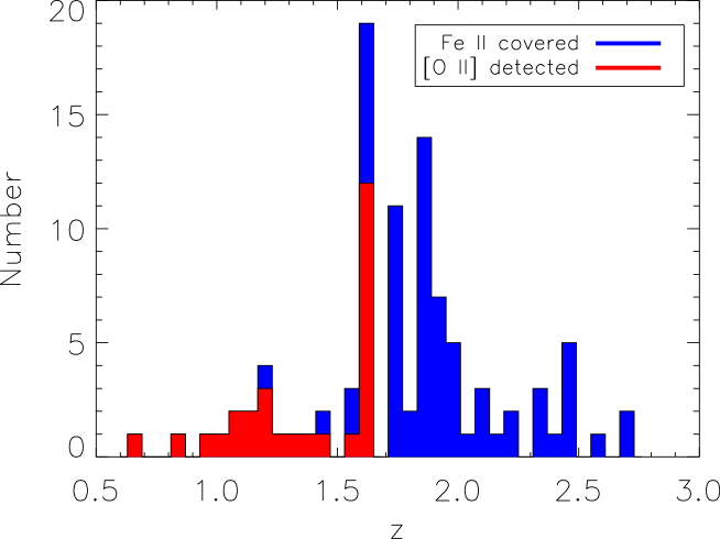
Figure 1: Distribution of redshifts of GMASS galaxies. Blue: all objects covering $2200-2700\AA$ in rest frame. Red: objects covering $2200-2700\AA$ and with [O II] $3727$ detection.

For the remaining galaxies in the sample the redshift of the [O II] could not be measured, either because the line is outside of the available spectral range or because the S/N ratio was poor (typically due to overlapping OH night sky emission lines). To measure their redshifts we have stacked the spectra from Sample [O II] to generate a high S/N template spectrum, and then we have used the IRAF task XCSAO to cross–correlate this template with the spectra with no [O II]. For these galaxies the cross–correlation determines the redshift primarily from interstellar absorption features, and since the velocity of winds in the individual galaxies is in general different from that of the template spectrum (which represents average wind properties), the redshifts measured in this way deviate from systemic by a random amount of the order of a few hundred km/s. We have visually inspected the spectra with cross-correlation redshift, and we have excluded low quality spectra, i.e. those with less than three identified features. The resulting sample of cross–correlation redshifts contains 98 galaxies, and we will refer to this sub sample as “Sample Abs” hereafter. Thus, in total, we have redshifts for 141 galaxies, and for 97 of them the spectra cover the Fe II multiplets at $2300-2600$ Å. These 97 galaxies form the final sample that we have used in our subsequent analysis. Their redshift distribution is shown in Figure 1. The clear spike shows that a large number of the galaxies belong to the large structure at $z=1.6$ studied by Kurk et al. (2009), who conclude that such an over-density of galaxies represents a proto–cluster.

The uncertainty in the measure of the redshift of Sample [O II] galaxies is dominated by the uncertainty in the determination of the line centroid, which is estimated from the covariance matrices during Gaussian fit. The corresponding errors are small, less than 25km/s. For the cross–correlated redshifts, we have followed Tonry and Davis(1979) and used the XCSAO package to calculate the error as a function of the r statistics of the correlation peak (Kurtz & Mink et al. 1998). Assuming sinusoidal noise with a half width of the sinusoid equal to the half-width of the correlation peak, the mean error in the estimation of the peak of the correlation function is: $err=\frac{3w}{8(1+r)}$, where $w$ is the FWHM of the correlation peak and r is the ratio of the correlation peak height to the amplitude of the antisymmetric noise. The effectiveness of this assumption has been discussed in detail by Kurtz & Mink (1998). In our case, the value of the uncertainty is $100\sim 200km/s$, but we also have to consider an additional source of uncertainty due to the variation in outflow velocities, which is also in the range $100\sim 200km/s$ (Erb et al. 2012).

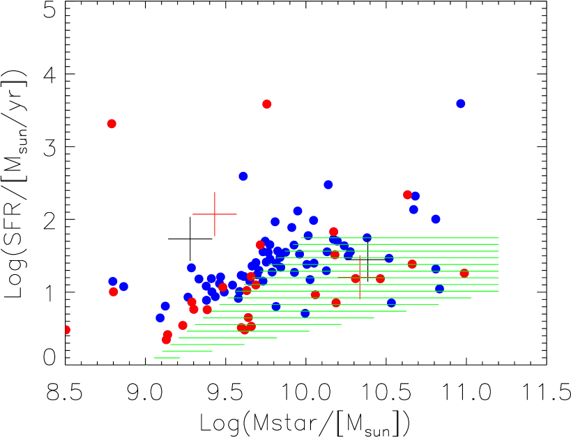
Figure 2: $SFR-M_{*}$ diagram. Red dots indicate detection of [O II] and blue dots indicate non-detection of [O II] . The green shadowed area defines the region of DEEP2 sample studied by Kornei et al. (2012) and Kornei et al. (2013). The black plus signs represent mean values of the low mass and high mass subsample defined in Erb et al. (2012), the red plus signs represent mean values of their low age and high age subsample.

In Figure 2, we show the SFR-M* diagram for the 97 GMASS galaxies in our sample overplotted with the region defined by the DEEP2 sample studied by Kornei et al. (2012, 2013). In this work SFR and $M_{*}$ are estimated based on the Salpeter IMF, therefore both are scaled down by a factor of 1.8 in order to be compared with previous results based on the Chabrier IMF. The mean locations of the low mass and high mass subsamples and low age and high age subsamples studied by Erb et al (2012) are also plotted in the figure for comparison. While the range of the GMASS galaxies overlaps with those of the other studies, for given stellar mass the GMASS sample appears to include larger numbers of galaxies with larger SFR relative to the DEEP2 ones, which is very likely due to the higher redshifts of the former.

The galaxies in the sample by Erb et al. (2012) cover a range of stellar mass that is lower than that of the GMASS galaxies, even if the redshifts of the two samples are similar. This is very likely the result of the UV selection of the former and of the mid–IR selection of the latter. At the low mass end the GMASS sample is sparse in the region covered by the Erb et al.’s sample.

2.3 Averaging Galaxy Spectra

We have averaged the spectra of both Sample [O II] and Sample Abs separately, and then combined both. Prior to averaging, the spectra are shifted back to their rest frame and are linearly interpolated to a uniform grid with $0.5\AA$/pixel. The rest frame wavelength coverage of each spectrum is recorded, after being trimmed of low S/N edges, for further selections of subsamples with constrained rest-wavelength coverage. To avoid being biased towards bright objects, which have higher S/N and higher flux density, individual spectra are normalized before averaging. In this study, we focus on Fe II and Mg II lines between $2300\AA$ and $2900\AA$. We extract three spectral windows from each individual spectrum, $2220-2460\AA$, $2505-2690\AA$ and $2740-2870\AA$ (band 1, 2 and 3, respectively). In each window, the individual spectrum is normalized by the continuum determined by fitting a straight line to the two spectral regions adjacent to the features: [$2220-2305\AA$, $2415-2460\AA$] for band 1, [$2505-2550$, $2640-2690$] for band 2 and [$2740-2780$, $2815-2840$] for band 3. Finally, we calculate the median for each pixel to derive a “representative” spectrum of our sample. Throughout this work, we have estimated the uncertainty of any measurement based on the “representative” or average spectra from the variance of 200 boostrap realizations of the data.

Figure 3 shows the extracted windows from the average spectra around the Fe II multiplets, and around the $2800\AA$ Mg II doublet. Blueshifted Fe II and Mg II are clearly present in both samples, with velocity of maximum absorption in the range $\sim 100-200$ km/s. The absorption lines are fairly separated, with slight blending for Fe II $2374,2382$ ($\Delta v=1050km/s$) and Mg II$2796,2803$ ($\Delta v=768km/s$). This is not simply due to the relatively low resolution of our spectra ($\sim 450$ km/s), but must be due to the broad blue wings of the absorption lines characterizing outflow kinematics.

Four emission features are clearly present around the wavelengths of Fe II absorption lines at $2365$, $2396$, $2612$ and $2626$ Å, as marked in Figure 3. The detection of these emission features in the spectra of star–forming galaxies has only been recently reported (Rubin et al. 2011; P11; Coil et al. 2011). As suggested by these authors, emission features around Fe II absorption lines could simply be explained as Fe II* fluorescence emissions, which are downward transitions to excited fine structure levels from the same upper levels of the observed Fe II absorptions. The high S/N achieved by averaging our spectra together offers an ideal chance to study the origin of these emission features, and in Section 4 we examine whether indeed photon scattering could be the primary excitation mechanism for Fe II* emissions.

3 Fe II Absorptions in GMASS Galaxies

3.1 Absorption and Continuum Fluorescence

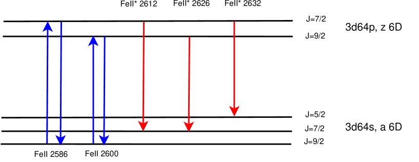
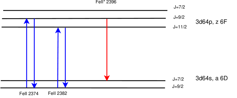
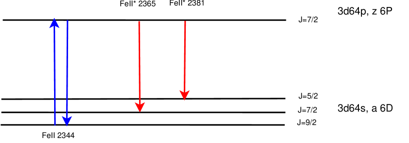
Figure 4: Energy level diagram of Fe II/Fe II* transitions. Resonance lines are shown in blue and fluorescence transitions are shown in Red.

Similarly to Figure 1 in P11, we show the energy level diagrams of Fe II and associated Fe II* lines in Figure 4. We use the atomic data from Morton (2003). The five observed Fe II resonance lines in absorption are associated with six downward permitted transitions to excited fine structure levels (also called fluorescence transitions), respectively. These transitions are :Fe II $2344.2$ $\rightarrow$ Fe II* $2365.6$/Fe II* $2381.5$; Fe II $2374.5$ $\rightarrow$ Fe II* $2396.4$; Fe II $2586.7$ $\rightarrow$ Fe II* $2612.7$/Fe II* $2632.1$; Fe II $2600.2$ $\rightarrow$ Fe II* $2626.5$. Note that for Fe II $2382.8$, no fluorescence downward transition is permitted. The transition Fe II* $2381$ is blended with Fe II $2382$, and the Fe II* $2632$ is undetected in our average spectra. The null-detection of Fe II* $2632$ could pose a potential challenge to the picture shown above, and we will come back to this point in Section 4.2.

Unless lower excited levels are significantly populated, the cold gas should be optically thin to the Fe II* emission, and once these photons are produced they can escape the interstellar medium or outflow winds. This suggests that the Fe II* lines should be observed at systemic velocity, since in a symmetric wind, the Fe II* lines from the advancing and receding parts of the wind are both received by the observer (Rubin et al. 2011).

3.2 Classification of Fe II Absorption Lines

In the following sections we discuss the dependence of the EW(Fe II) and EW(Mg II) on the location of Fe II absorbing medium and the wind kinematics and discuss the implications. We start by discussing the profile of the Fe II absorption lines.

Two parameters control the propagation of resonance photons through the ISM, namely the lower level oscillator strength of that transition, $f_{l}$, which determines how frequently a photon is absorbed, and the probability of fluorescence, which measures the likelihood that the random walk of resonant photons in the nebula is terminated by an absorption event. The probability of fluorescence is defined as:

$$P_{fluo}(FeII_{i})=\frac{\sum_{j}A_{ul}(FeII*_{j})}{\sum_{j}{A_{ul}(FeII*_{j})}+{A_{ul}(FeII_{i})}},$$ (1)

where $A_{ul}(FeII*_{j})$ and $A_{ul}(FeII_{i})$ are the Einstein coefficient for spontaneous emission of fluorescence transition Fe II*_j and resonance transition Fe II_j, respectively. Thus, $P_{fluo}(FeII_{i})$ is simply the possibility for a resonance photon Fe II_i to be re-emitted as a Fe II* photon after an absorption event.

$P_{fluo}$ and $f_{l}$ of Fe II transitions are listed in Table 2. For the Fe II absorption lines, line profiles are entirely controlled by $f_{l}$ and $P_{fluo}$. Before discussing how this is achieved, we first point out that there exists a monotonic decreasing relationship between $f_{l}$ and $P_{fluo}$ for the five Fe II transitions of concern in this study, which is shown in Figure 5. The Fe II transitions with higher oscillator strength always have lower $P_{fluo}$, and this relationship can be approximated as $f_{l}\times P_{fluo}\approx 0.03$.

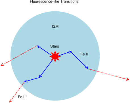
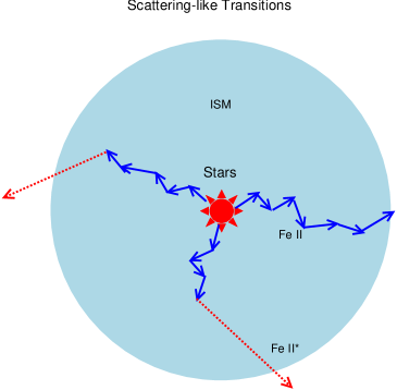
Figure 6: Illustration of two different types of radiative transfer: fluorescence-like and scattering-like.

Figure 5 shows that, Fe II transitions can be placed on a monotonic sequence: Transitions on the left-top corner have low $f_{l}$ and high $P_{fluo}$, resonance photons of these transitions are less absorbed, each absorption is likely followed by a re-emission of Fe II* photon. We refer to them hereafter as “fluorescence-like” transitions. At the opposite end, transitions on the right–bottom corner have high $f_{l}$ and low $P_{fluo}$ and thus resonance photons of these transitions are more frequently absorbed but less frequently or never give rise to fluorescence transitions. We refer to them hereafter as “scattering-like” transitions. In an homogeneous, dustless ISM, the propagation of these two types of resonance photons is illustrated by Figure 6. We note here again that Figure 6 only represents a special case in a static ISM. The propagation of photons in an outflow wind further depends on velocity gradient in the flowing fluid, as continuum photons are absorbed in regions those where the co-moving wavelength of photons are Doppler shifted to local resonance wavelength.

3.3 Equivalent widths of Absorption Lines

To measure the EWs of Fe II and Mg II absorption lines, we combined Sample [O II] and Sample Abs to achieve higher S/N ratio. We used only the 83 spectra with common coverage the rest frame spectral range $2200-2900$ Å. We fit a Gaussian profile to each absorption line, since several lines are slightly blended (Fe II $2586/2600$ and Mg II$2796/2803$) and can not be measured by direct integration of each line’s spectrum. Although the intrinsic line profile should be asymmetric due to the outflow, our spectral resolution is too low to observe this effect, and the absorption line profiles show small deviation from the Gaussian one. The bootstrap resamplings of the spectra show that internal errors of our measures are $\approx 10$% or less. The results are listed in Table 2.

The oscillator strengths of the five Fe II lines range over one order of magnitude, and including the Mg II doublet further extended this range by a factor of 2. In contrast, their EWs span a relatively narrow range from $1.5-2.2$. The line with the lowest EW, Fe II $2374$, also has the lowest oscillator strength $f_{l}=0.0313$. This has been interpreted in previous work as evidence that the lines are saturated. However, as shown in P11, Fig 5, in an expanding wind model the presence of scattered emission could mimic the effect of partial covering of the continuum source. This is because a) in an outflow wind, transitions with higher $f_{l}$ are associated with stronger redshifted P-cygni emission features from back-scattered photons, which are likely blended with absorption lines in our low resolution, average spectrum. We will show evidence of this effect in Section 3.7; b) absorption lines with high $f_{l}$ could be “re-filled” by scattered photons. According to the $P_{fluo}-f_{l}$ diagram, low $f_{l}$ lines are efficiently converted to fluorescence photons instead of being resonantly scattered.

It is unclear to us whether these effects can reproduce the narrow range of EWs that we observed, but it is important to keep in mind that that contributions from unsaturated absorption lines should not be ignored.

3.4 Modeling Line Profiles

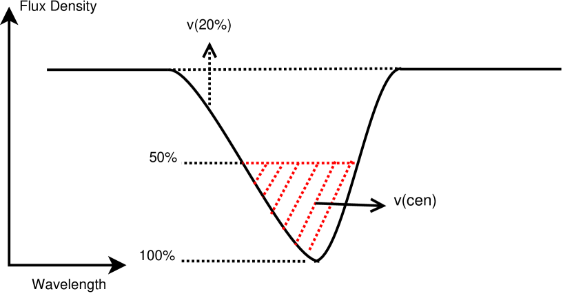
Figure 7: Illustration of how we quantify line profile: $v_{20\%}$ and $v_{cen}$.

In this work, we model line profiles by means of a two parameter representation. As illustrated by Figure 7, first we measure the extent of blue line wing by $v_{20\%}$, the velocity where $20\%$ of the continuum is absorbed. We then calculate the velocity centroid of absorption as:

$$\lambda_{cen}=\frac{\int_{\lambda_{(50\%blue)}}^{\lambda_{(50\%red)}}\tau(\lambda)\cdot\lambda\mathrm{d}\lambda}{\int_{\lambda_{(50\%blue)}}^{\lambda_{(50\%red)}}\tau(\lambda)\mathrm{d}\lambda}$$ (2)

$$v_{cen}=c\cdot\frac{\lambda_{cen}-\lambda_{rest}}{\lambda_{rest}},$$ (3)

where $\lambda_{(50\%blue)}$ and $\lambda_{(50\%red)}$ are the wavelengths at which the depth of absorption trough decrease to $50\%$ of the peak depth on the blue side and the red side, respectively. The wavelength centroid $\lambda_{cen}$ is calculated between $\lambda_{(50\%blue)}$ and $\lambda_{(50\%blue)}$, weighted by apparent optical depth $\tau(\lambda)$. $\tau(\lambda)=\log(1-\frac{F(\lambda)}{F_{c}(\lambda)})$, where $1-\frac{F(\lambda)}{F_{c}(\lambda)}$ is the depth of absorption trough at wavelength $\lambda$.

In the following sections, we discuss how $v_{20\%}$ and $v_{cen}$ depend on locations of Fe II in $P_{fluo}-{f_{l}}$ diagram.

3.5 Dependence of $v_{20\%}$ on Line Properties

Consider an expanding wind with increasing velocity and decreasing density moving away from the galactic center. To first order, $v_{20\%}$ increases with $f_{l}$, since lines with high $f_{l}$ can trace down to low density regions at large radii and hence higher velocities. The five Fe II absorption lines considered here span a factor of 10 in $f_{l}$, suggesting a substantial spread in the extent of line wing. On the other hand, at a fixed oscillator strength, low $P_{fluo}$ lines suffer more from scattered refilling and thus should be less extended in velocity to the blue. Therefore, to a certain degree, due to the inverse $P_{fluo}-f_{l}$ relationship, the increasing of the absorption EW at higher oscillator strengths is counter-blanced by the increasing of the scattered refilling. However, it is easy to perceive that the scattered refilling is still a secondary effect in shaping line profiles, since any scattering must be initiated by a resonance absorption.

3.6 Dependence of $v_{cen}$ on Line Properties

If the re-shaping of absorption lines by re-emitted photons is ignored, $v_{cen}$ simply traces the highest density region of the wind, which should be constant for different Fe II lines. However, P11 shows that the peak velocity of absorption lines could be severely blended with nearby, redshifted P-cygni emissions, which is built from photons scattered by receding part of wind. This effect could be even more significant in our low resolution data. “Scattering-like” transitions are associated with strong P-cygni emissions, as their corresponding resonance photons are more scattered and less fluoresced. For these transitions, the P-cygni emission is blended with absorption line and “pushes” the line centroid $v_{cen}$ toward shorter wavelengths. At the opposite, “Fluorescence-like” transitions suffer less contamination from P-cygni emission, as their corresponding photons have long mean free path and high $P_{fluo}$. Therefore $v_{cen}$ can also be positively correlated with $f_{l}$. This effect has been clearly demonstrated in P11, Figure 23.

3.7 Profiles of Fe II and Mg II Absorption Lines in Average Spectrum

Similar to previous analyses, we combined Sample [O II] and Sample Abs and selected galaxies with wavelength coverage $2200-2700$ Å. The average spectra are first smoothed using a boxcar of 3 pixels. Note that, although Sample Abs is characterized by large uncertainties in systematic redshifts, which are estimated from cross-correlation, since our primary interest is relative differences in line profiles, as long as our comparison is carried out on the same set of spectra, the uncertainty of the absolute systemic redshift, which shifts all lines by an equal amount, is canceled out.

At our spectral resolution, the Fe II $2382$ absorption line is blended with the Fe II* $2381$ emission. Since Fe II* $2381$ and Fe II* $2365$ share same upper level, we scale Fe II* $2365$ to remove Fe II* $2381$ component from Fe II $2382$. To do this, we first select a spectral window, $-700-600$ km/s wide, around Fe II* $2365$, then we scale the emission line profile in this window by the ratio of Einstein A Coefficient $A_{2381}/A_{2365}$, and subtract it from the spectra. Without this correction, $v_{cen}$ of Fe II $2382$ would be lower by $10-20$ km/s. We plot $v_{cen}$ and $v_{20\%}$ of Fe II in Figure 8 as a function of $f_{l}$. For lines of low $f_{l}$, such as Fe II $2374$, Fe II $2586$, FeII $2374$, the relationship between $v_{cen}$ and $v_{20\%}$ with $f_{l}$ is in agreement with the discussion above—assuming an accelerating, smooth wind, both increase with $f_{l}$. This trend starts to flatten at high velocities.

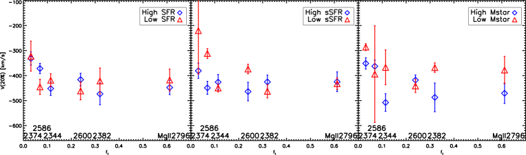
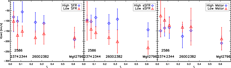
Figure 9: Comparing $v_{20\%}$ (top panel) and $v_{cen}$ (lower panel) of subsamples with high/low SFR, sSFR and stellar mass, only galaxies with [O II] 3727 detection are included. Red triangles represent low SFR/sSFR/stellar mass, blue diamonds represent high SFR/sSFR/stellar mass.

To further explore kinematic properties of Fe II, we selected galaxies from Sample [O II] that have common coverage of the spectral range $2200-2900$ Å. We have then divided these 28 galaxies, for which accurate system redshift is available, into two subsamples by their median star–formation rate (SFR), $18.95M_{\odot}yr^{-1}$, specific star formation rate (sSFR), $-8.62yr^{-1}$, and stellar mass, $10^{9.9}M_{\odot}$, respectively, and have averaged them. We compare the values of $v_{cen}$ and $v_{20\%}$ of each pair of subsamples in Figure 9, $v_{20\%}$ and $v_{cen}$ of Mg II 2796 are also plotted here. Note that since Mg II$2803$ is blended with Mg II$2796$, $v_{20\%}$ of Mg II$2803$ is not measurable in average spectra.

Similar to terminal velocity, $v_{20\%}$ strongly depends on the high–velocity components of ourflowing fluids. Several previous studies have found that $v_{terminal}$ scales roughly with the star–formation rate as SFR^0.3 for Mg II doublet (Martin et al. 2005; Weiner et al. 2009; Banerji et al. 2011), suggesting that outflow wind in more intensively star–forming galaxies are accelerated to higher speed. Using our subsample of 28 galaxies, however, we find that $v_{20\%}$ has a stronger dependence on stellar mass and on specific star–formation rate, as systematic offsets between high M_∗/sSFR and low M_∗/sSFR samples are higher than $1\sigma$ uncertainty of $v_{20\%}$, this might suggest that gravity also plays an important in the kinematics of the wind. On the other hand, $v_{cen}$ is possiblly related to sSFR, as indicated by systematic offsets between subsamples. Note that unlike $v_{20\%}$, $v_{cen}$ increases with decreasing sSFR.

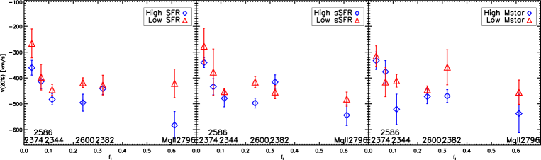
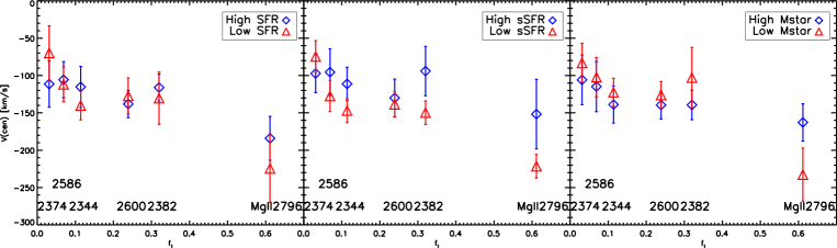
Figure 10: Similar to Figure 9, but include galaxies with redshifts determined from cross-correlation.

The velocities measured in the average spectra of Sample [O II] have large uncertainties due to the limited sample size. Therefore we have repeated the above analysis including another 55 galaxies from Sample Abs with coverage of the $2200-2900\AA$ spectral range. The results are shown in Figure 10. Distributions of $v_{20\%}$ and $v_{cen}$ are in agreement with Figure 9. Note that, since galaxies in Sample Abs do not have accurate systemic redshift estimates, only relative differences in $v_{20\%}$ and $v_{cen}$ measured from the same set of spectra are meaningful, vertical offsets between cross-correlated subsamples could be potentially dominated by transitions other than Fe II and Mg II.

We also find that, there is a trend of increasing EW(Mg II) and EW(Fe II) in massive and high–SFR galaxies observed in GMASS galaxies, and this is consistent with previous studies (Erb et al. 2012, Kornei et al. 2012, 2013, Martin et al.2012). To compare our results with that derived by Erb et al. (2012), which are based on a sample with similar redshift range, we use exactly the same criteria by Erb et al. (2012) to split galaxies into subsamples by their M_∗, SFR, E(B-V) and age. The sample of Erb et al. (2012) is selected based on the rest UV colors of the galaxies (the so–called “BM” color criteria) and $R$ magnitude. In their study, composite spectra are constructed based on galaxies properties of SFR, M*, Age and E(B-V). The trend between the profiles of absorption lines in the wind and the sSFR has not been directly studied by Erb et al. (2012). However, their comparison based on stellar age shows that EW(Mg II) is enhanced in old and massive galaxies, which also exhibit a mean sSFR 0.8 dex lower than the young and low–mass galaxies.

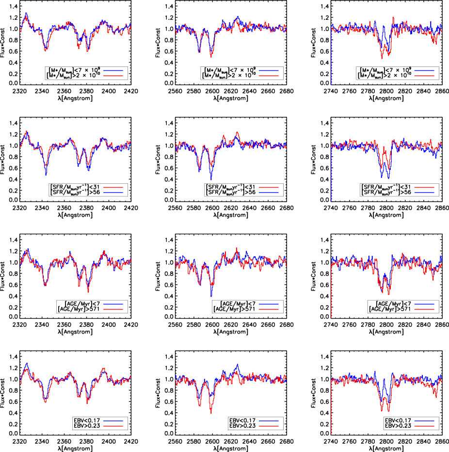
Figure 11: The galaxies are split into subsamples by $M_{*}$, SFR, age and E$(B-V)$, using the same criteria used by Erb et al. (2012). The composite spectra of each pair of subsamples with low/high $M_{*}$, SFR, age and E$(B-V)$ are plotted together for comparison.

The composite spectra of each pair of subsamples are plotted in comparison in Figure 11. The mean SFR/$M_{*}$/Age/E(B-V) of each subsample are listed in Table 6 and the EWs of Fe II and Mg II are listed in Table 7. Again, since Erb et al. use the Chabrier IMF, we scale up their criteria of SFR and M* by a factor of 1.8 since our measurements are based on the Salpeter IMF. The typical S/N of composite spectra is $17-27/pixel$. The general trends of Mg II are increasing EWs in massive/high SFR galaxies. Also, MgII absorption is slightly weaker in the young-age subsample than in the old-age subsample, both in agreement with Erb et al. (2012). On the other hand, EWs of the Fe II absorptions show smaller variation across subsamples. All these trends are similar to that found by Erb et al. (2012) and Kornei et al. (2012).

4 Fe II* Emissions in GMASS Galaxies

4.1 Relative Line Strengths of Fe II*

Since emission features around Fe II are not resolved in our low resolution data, the possibility can not be ruled out that the Fe II* emission features are blended with other Fe II transitions. The energy level configuration of Fe⁺ is among the most complex among ion species in astrophysical environments, as Fe⁺ has 6 valence electrons in its outermost shell and exhibit substantial fine structure splittings. If Fe⁺ is excited by mechanisms other than continuum fluorescence —which is true in AGN broad line regions— the emission features could be broad and could be associated with thousands of transitions (Vestergaard & Wilkes 2001, Sigut & Pradhan 2003). In this work, we are not trying to explore other possible excitation mechanisms (collision excitation, recombination, etc.), and we focus only on continuum fluorescence and examine whether this simple excitation mechanism offers a satisfactory explanation for the observed Fe II* emissions in $z=1.0-2.6$ galaxies.

Assuming a flat incident continuum between $2300-2700\AA$, the EW of an Fe II* emission line is proportional to the fraction of the incident resonance photons being eventually fluoresced through that particular Fe II* transition. For a transition Fe II*_i, we define the total conversion fraction as

$$F(FeII*_{i})=\frac{N_{fluo}(FeII*_{i})}{N_{resonance}(FeII_{i})},$$ (4)

where $N_{resonance}(FeII_{i})$ is the number of the incident resonance photons associated with the $FeII*_{i}$ transition, and $N_{fluo}(FeII*_{i})$ is the number of the Fe II$*_{i}$ photons being eventually produced. For a single absorption event, $F(FeII*_{i})$=$P_{abs,single}(FeII*_{i})\times P_{fluo,single}(FeII*_{i})$, where $P_{abs,single}$ is the probability of absorption and $P_{fluo,single}$ has been defined by Eq(1). For multiple absorption events, the $i_{th}$ absorption event and the ${i+1}_{th}$ absorption event are not independent, and $F(FeII*_{i})$ depends on the specific process of radiative transfer.

This problem could be simplified in two extreme cases: the optically thick limit and the optically thin limit. In the optically thick limit, after multiple absorption and re-mission, all resonance photons are eventually fluoresced. If, for instance, Fe II*_i is the only permitted fluorescence transition from its upper level, $F(FeII*_{i})=100\%$. Otherwise, decaying through other fluorescence transition must be accounted. Without loss of generality, the total conversion fraction for Fe II* in the optically thick limit is:

$$F_{thick}(FeII*_{i})=\frac{A_{ul}(FeII*_{i})}{\sum_{j}{A_{ul}(FeII*_{j})}},$$ (5)

where $A_{ul}(FeII*_{i})$ is the Einstein coefficient for spontaneous de-excitation to excited fine structure levels and $\sum_{j}{A_{ul}(FeII*_{j})}$ is the sum of $A_{ul}$ coefficients for all permitted Fe II* transitions decaying from the same upper level as $FeII*_{i}$.

In the optically thin limit, the total conversion fraction of Fe II*_i is

$$F_{thin}(FeII*_{i})=P_{abs,single}(FeII*_{i})\times P_{fluo,single}(FeII*_{i}).$$ (6)

Here $P_{abs,single}\propto f_{l}(FeII_{i})$, where $f_{l}(FeII_{i})$ is the oscillator strength of Fe II_i.

In Figure 12 we show the ratios $\frac{EW(FeII*_{i})}{F_{thin}(FeII*_{i})}$ and $\frac{EW(FeII*_{i})}{F_{thick}(FeII*_{i})}$ for all Fe II* transitions. The ratios are re-normalized such that the average ratio in each case equals 1 ($AVG(\frac{EW}{F_{thin}})=1$ and $AVG(\frac{EW}{F_{thick}})=1$). To measure EW(Fe II, we averaged all spectra which have common coverage of the range $2200-2700$ Å. The EWs are measured by integrating the line profile within specified wavelength ranges, as listed in Table 3. To avoid contamination from the neighboring Fe II absorption lines, each Fe II absorption line is fitted by a Gaussian profile and subtracted from the original spectra prior to the integration. For a flat continuum, the ratio between EW and conversion fraction $\frac{EW(FeII*_{i})}{F(FeII*_{i})}$ should be a constant.

The relative conversion fractions are $F(2365):F(2396):F(2612):F(2626)=0.66:1.0:0.66:1.0$ in the optically thick limit, and $F(2365):F(2396):F(2612):F(2626)=0.26:0.27:0.31:0.30$ in the optically thin limit. In the optically thin limit, the similar conversion fractions among Fe II* lines result from the inverse relationship between $P_{single}(FeII*_{j})$ and $f_{l}(FeII*_{j})$ as illustrated by Fig 5, $P_{single}(FeII*_{j})*f_{l}(FeII*_{j})\approx 0.03$, which basically states that lines that are more absorbed are less fluoresced. This effect leads to a roughly constant line ratio with varying optical depth. We find that in P11, all except two models predict the line ratio of Fe II*2612 and 2626 that fall between the two limits discussed here. These two exceptions have extreme physical conditions, namely a bipolar wind with small opening angle ($45^{\circ}$) and sharp edges, and a model which simply ignores resonant trapping. Since the relative strengths of Fe II* lines are nearly constant within a wide range of column density, they are poor diagnostics of density gradients. Nevertheless, since this test shows that the ratios of Fe II* lines agree with the scenario of continuum fluorescence, no other mechanism is really necessarily required to explain their excitation mechanism.

There is, however, an exception to this picture. As will be discussed in the next section, the Fe II* transition F(2632) is not detected in the average spectrum of the whole sample. And this null detection is not simply a result of low S/N ratio.

4.2 Null Detection of Fe II* 2632

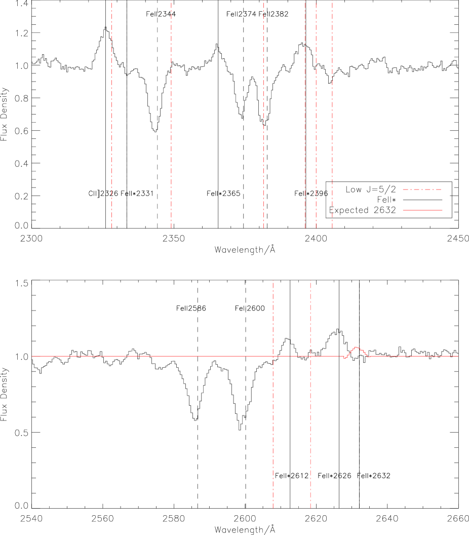
Figure 13: Same as Figure 3, with estimated Fe II* $2632$ emission being shown in solid red. Transitions with lower level J=5/2 are marked by red dash-dot line.

Considering the large EWs of Fe II resonance lines ($|EW|>1.3\AA$), one might expect that all Fe II* lines associated with resonance transitions should be present in the high S/N average spectrum, except Fe II* $2381$, which is blended with Fe II $2382$. The emission line Fe II* $2632$, however, is undetected in our average spectra. Since Fe II* $2632$ decays from the same upper level as Fe II* 2612, the expected strength of Fe II* 2632 can be estimated by scaling Fe II* $2612$ with the ratio of their Einstein A Coefficients. To do this, we have extracted the profile of Fe II* 2612 from a velocity window $[-550-400]$ km/s and multiplied it by $A_{ul}(2632)/A_{ul}(2612)$. The expected profile is shown in Figure 13, where we see that the 3-sigma detection limit of the EW of the 2632 emission is $0.1\AA$ while the expected EW estimated for the 2612 emission is $0.2\AA$.

One possibility for the lack of detection is that the lower level of Fe II* $2632$, $J=5/2$, is heavily populated through non-radiative excitations. If this is true, we should also detect other absorption lines arising from the same lower level. All transitions with lower level $J=5/2$ and $f_{l}$ $>0.02$ are marked in Figure 13. No isolated absorption line corresponding to these transitions is clearly detected. Especially, Fe II* $2405$ and Fe II* $2400$ have $f_{l}$ $2.7$ and $1.4$ times as that of Fe II* $2632$ and so one should expect obvious absorption features at these wavelengths if $J=5/2$ is significantly occupied. We conclude, therefore, that it is unlikely that the null detection is the result of heavily populated lower level.

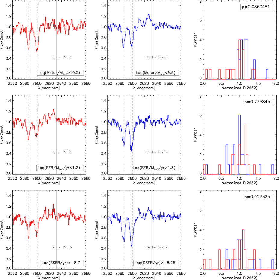
Figure 14: Comparing Fe II* 2632 in subsamples split by M_∗/SFR/sSFR. Left Panels show subsamples with high stellar mass, low SFR and low sSFR, from top to bottom, respectively. Right panels show low stellar mass, high SFR and high sSFR. We perform a K-S test on each pair of subsamples to examine if there is a significant segregation of F(2632). We see a possible separation of Fe II* 2632 only in M*-split subsamples, with a significance level of $8.6\%$ rejecting the null hypothesis that the two distributions are drawn from the same parent sample.

Fe II* $2632$ emission feature could also be obscured by underlying absorption features in stellar continuum. In passive galaxies, the most prominent stellar feature around Fe II* $2632$ is the B2640 continuum break (Spinrad 1997, Cimatti et al. 2004), which primarily reflects UV1 close spaced Fe II resonance multiplets on the shorter wavelength side of $2640\AA$ produced in photosphere of late F and G type stars. Stellar absorption is actually found to be significant for passive galaxies in the GMASS sample (Cimatti et al. 2008). To examine whether Fe II* $2632$ could be obscured by the absorption features in our average spectrum, we compare in Figure 14 the average spectra of galaxies in subsamples with the highest half and lowest half of stellar mass, SFR, and sSFR. In the last column of Figure 14, the distributions of single-pixel continuum-normalized flux densities measured in individual spectra at $2632\AA$ are also plotted for comparison. We perform a K-S test on each pair of subsamples to examine if there is a significant segregation of F(2632). We see a possible separation of Fe II* 2632 only in M*-split subsamples, with a significance level of $8.6\%$ rejecting the null hypothesis that the two distributions are drawn from the same parent sample. In SFR and sSFR divided subsamples, Fe II* 2632 show no statistically significant separation.

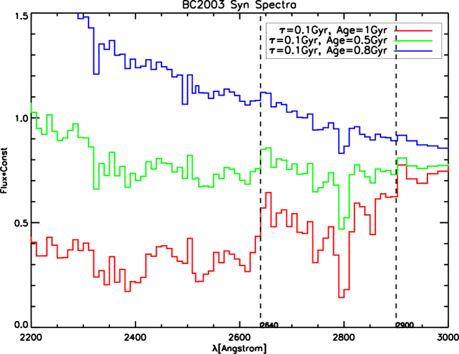
Figure 15: Synthesized spectra generated from BC03 model. An exponential decaying star-formation history with an e-folding time of 0.1 Gyr is assumed here. The spectra are shown for three different ages, $0.3,0.5$ and $1Gyr$. The stellar Fe II absorptions and 2632 break are less prominent in younger galaxies.

The intensity of the B2640 break should be related to the location of the galaxy in Color-Magnitude Diagram (Spinrad et al. 1997). For a subsample of passive GMASS galaxies, Cimatti et al. (2008) estimate a decrease of $59\%$ in the continuum level across the $2640$ Å break. Starforming galaxies, however, should have a less pronounced break. Nevertheless, it cannot be ruled out that stellar absorption responsible for this discontinuity is potentially sufficient to suppress the FeII* $2632$ emission. We show the synthesized spectra generated from the BC03 templates in Figure 15. For a galaxy with Age=0.3-0.5 Gyr, the continuum discontinuity is between a few to 10 percent. This is comparable to the expected intensity of Fe II* 2632 estimated from Fe II* 2612, which has a peak flux density lower than $10\%$ of the continuum level, as shown in Figure 13.

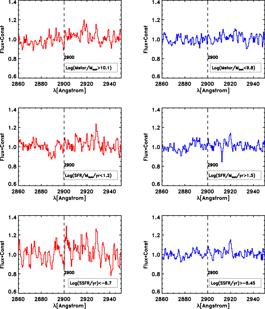
Figure 16: Comparing B2900 of subsamples with low/high M_∗/SFR/sSFR. Left Panels show subsamples with high stellar mass, low SFR and low sSFR, from top to bottom, respectively. Right panels show low stellar mass, high SFR and high sSFR.

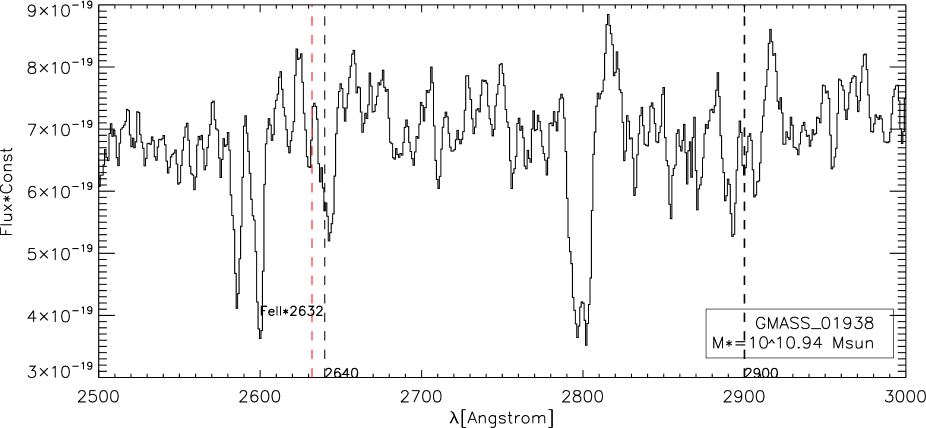
Figure 17: The spectrum of GMASS01938, which has a stellar mass of $10^{10.94}M_{\odot}$. Absorption features blueward of $2640\AA$ and $2900\AA$ are possibly present.

The S/N ratios and the spectral resolution of the GMASS data do not allow us to decompose the stellar absorption and the FeII* $2632$ emission. One way to further test this scenario is to examine the B2900 break, another continuum break caused by similar metal absorptions in F and G-type stars. (i.e. FeII, FeI etc. Heap et al. 1998). In Figure 16, we compare the strengths of B2900 break in the average spectra of the lowest half and the highest half sSFR, SFR and stellar mass subsamples. In order to retain this feature of continuum break, we simply normalized each individual spectrum by its median value over the wavelength range $2820-2970\AA$ prior to coaddition, instead of normalizing each spectrum by its continuum. The high stellar mass and the low sSFR spectra do show signs of absorption blueward of $2900$ Å, which is absent in the average spectrum of the bluest galaxies. We also show a high S/N spectrum of one massive galaxy, GMASS-01938, in Figure 17. In this single case, absorption features are possibly present blueward of $2640\AA$ and $2900\AA$.

Another important question is whether stellar absorption features could contaminate other Fe II/Fe II* lines. As shown in Spinrad et al. (1997) and Cimatti et al. (2008), the troughs of stellar-originated resonance FeII absorptions in passive galaxies are shallower than the B2640 and B2900 discontinuities. In our co-added spectra, if the absence of the Fe II*2632 emission were due to stellar absorption lines blueward of B2640, these stellar absorptions should have a integrated intensity roughly equal to EW(Fe II* 2632). By scaling EW(Fe II* 2612), we estimate that EW(Fe II*2632)$\approx 0.2$ Å. The EWs of other less-significant stellar resonance absorption features are unlikely to be higher than this. It is still possible, however, that Fe II*2612 and Fe II*2626 are also suppressed by stellar absorptions. We do see signs of this possibility in our result, as will be discussed later in Section 4.4.

4.3 Stacking 2D Spectral Images

To explore the spatial extent of Fe II* emission we have stacked the 2D spectral images of individual galaxies. Similar to 1D spectral stacking, each image is interpolated to a uniform grid with $0.5\AA$/pixel in the dispersion direction after being shifted to the rest frame. We cut out three windows around Fe II* emissions from the 2D spectrum of each individual source, namely: $2350-2450$, $2550-2650$ and $2765-2865$Å. For each cut-out, pixels are averaged along the dispersion axis to produce a 1D distribution of surface brightness in the spatial direction, The peak of this 1D surface brightness distribution is identified through a 4th order polynomial fitting. Each cut-out is then regridded by linear interpolation to be centered at the fitted peak. We assume that the curvature of object trace is negligible within each narrow band. The fitted peak of the bluest band $2350-2450\AA$ and that of the reddest band $2765-2865\AA$ are typically offset by less than 1 pixel ($0.126^{\prime\prime}$), in no case more than 2 pixels, indicating a slope of up to 0.005 pixel/$\AA$. For each regridded cut-out, a continuum intensity is calculated by summing up all pixels within +/0.5” (4 pixels) from the center. The 2D cut-out is normalized by this continuum intensity. We use mean stack to create the final composite 2D spectra.

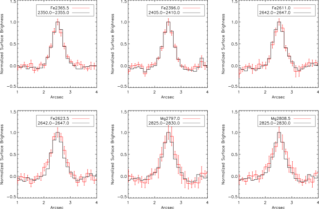
Figure 18: Top:Spatial distributions of Fe II* and MgII emissions (red) in stacked 2D spectral images comparing to that of continuum band (black). The final stacked image has a pixel scale of $0.5\AA$ along wavelength direction and a pixel of $0.126^{\prime\prime}$ along spatial direction. For each line, the plot corresponds to the wavelength with most extended distribution in a velocity range of approximately [$-500-500$] km/s around line center. Bottom: Residual signals of Fe II* and MgII emissions with continuum emission being subtracted.

Although in our average spectrum Fe II* lines peak approximately at systemic velocity, the velocities of spatially extended components of the Fe II* emission lines are necessarily systemic. To probe the most extended emission, we calculate FWHMs in spatial direction within a $-4$—$4\AA$ window around line center, pixel by pixel, and identify the wavelength with the highest FWHM, $\lambda_{ext}$. The spatial distribution of each Fe II* line at $\lambda_{ext}$ is overplotted with the average spatial distribution of a nearby continuum band in Figure 18. The uncertainties of each pixel are estimated from 200 bootstrap realsamplings of the 2D spectral images. No extended emission could be detected for any Fe II* lines. At the $1^{\prime\prime}$ spatial resolution of our data, this indicates that a large fraction of the Fe II* emission lines are within the central 4 kpc from the galactic center. Erb et al. (2012) report only marginal detections of extended Fe II* lines in stacked 2D spectral images, in agreement with our finding that the excess of extended Fe II* line is weak.

The compact Fe II* emission could be naturally explained by the low $f_{l}$ of resonance Fe II transitions. In P11, it is shown that the surface brightness of Fe II* line decreases by more than a order of magnitude to 4 kpc for a rapidly decreasing $r^{-2}$ density profile. This is also consistent with our previous result that Fe II resonance lines exhibit lower velocities than Mg II lines. For an accelerating wind, this could indicate that the Fe II absorption lines arise from an inner region. Recent studies (Rubin et al. 2011, Erb et al. 2012, Kornei et al. 2013, and Martin et al. 2013) show that in contrast with strong redshifted P-cygni emission lines usually seen for the Mg II doublet, Fe II transitions rarely present such feature, including Fe II $2382$, which, like Mg II, only involves pure scattering. A potential explanation for this absence of FeII scattered emission is that the Fe II absorptions and the Mg II absorptions originate from distinguishable regions of the ISM/wind. Such segregation could be caused by an evolution in ionization states of the Fe ions, as discussed by Martin et al. (2013), Fe irons are mainly in Fe⁺³ in low column density regions, while Mg ions could remain as Mg⁺⁺, since Mg III requires a much higher ionization potential.

Since the individual spectra are normalized by their continuum intensities before stacking, we cannot easily define a detection limit in terms of absolute surface brightness. Instead, we provide an upper limit relative to the continuum surface brightness in the co-added 2-D spectra. The 1-D continuum surface brightness is estimated from the mean of the central 9 pixels in the 1-D surface brightness distribution. The 3-sigma detection limit for Fe II* 2626 (usually the brightest Fe II* line) is $30\%$ of the continuum surface brightness over the entire profile.

4.4 Dependence of Fe II* Emission on Galaxy Properties

To further examine whether the intensities of Fe II* emission lines have any dependence on galaxy properties, such as stellar mass, SFR and sSFR, we split our 97 spectra into subsamples by their stellar population properties, and construct a median spectrum from each subsample. The intensity of the Fe II* emissions is quantified by their EWs, which are measured by integrating pixels within specified velocity ranges listed in Table 3. We average the spectra in the same way described in previous sections.

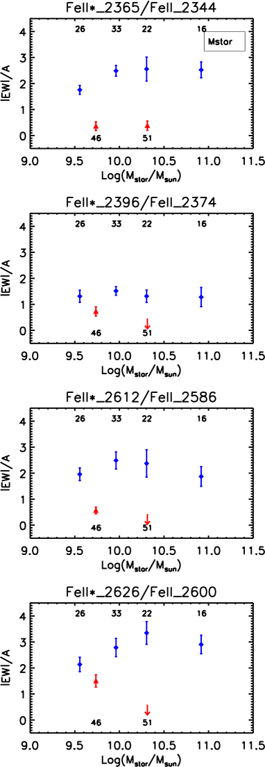
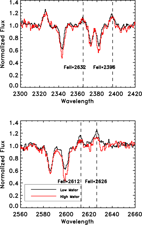
Figure 19: Left: EWs of Fe II (blue) and Fe II* lines (red) plotted as functions of M_∗, numbers of objects in each subsample are shown at bottom and top. Right: Comparing co-added spectra of low M_∗ (black) and that of high M_∗ (red).

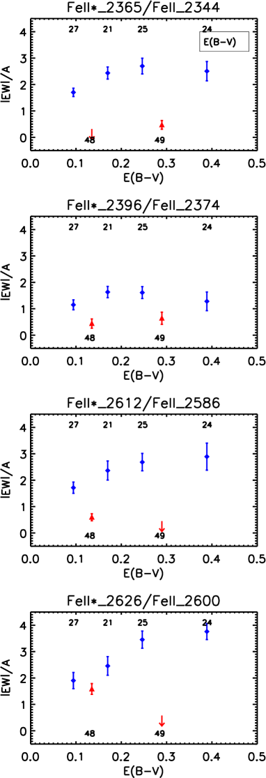
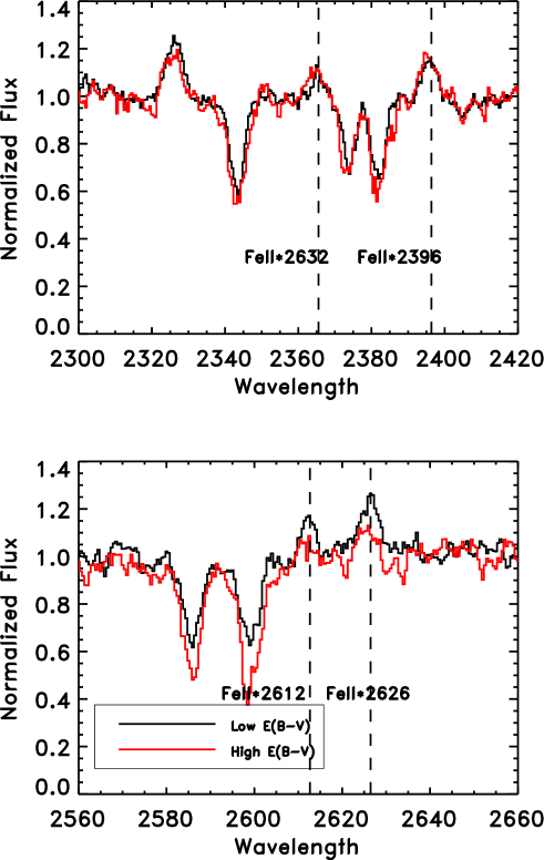
Figure 22: Left: EWs of Fe II (blue) and Fe II* lines (red) plotted as functions of E(B-V), numbers of objects in each subsample are shown at bottom and top. Right: Comparing co-added spectra of lower E(B-V) (black) and that of higher E(B-V) (red).

Specifically, the whole GMASS sample is split into 4 subsamples by each galaxy property (the stellar mass, SFR, sSFR and E(B-V)). We have chosen the subsamples to avoid spikes in the parameter distribution, and to assign each subsample with a roughly equal number of objects. For measuring the Fe II* emissions, which have smaller EWs and lower S/N ratios compared to the Fe II absorptions, the 4 subsamples are merged into 2. The EWs of the Fe II absorptions and the Fe II* emissions are plotted as a function of the median stellar mass/SFR/sSFR/E(B-V) in Figure 19 through Figure 22 (for the Fe II* emission lines the upper limit is $2\sigma$). In general, the dependence of both EW(Fe II) and EW(Fe II*) on galaxy properties is weak. For galaxies with increasing star formation activity, the strengths of Fe II* remains constant over more than one order of magnitude in SFR and sSFR. Coil et al. (2011), who report Fe II* detection in K+A galaxies with $|EW|>1\AA$, reach similar conclusions.

The EW of the Fe II* transitions, whenever detected, is $\sim 10\%-50\%$ of that of the associated Fe II absorption. For an ideal homologous, dustless wind, the conservation of the number of photons implies EW(em)$\approx$EW(abs). Since Fe II emission is not present in our average spectra, EW(Fe II*) should be approximately equal to EW(Fe II). A number of factors potentially capable of reducing the strength of emission lines have been discussed in P11, including bipolar morphology of the wind, dust extinction and slit losses. The null-detection of extended Fe II* casts doubt on slit losses as a reason for the attenuated emission. Dust extinction preferentially suppresses the red side of Fe II* emission, as photons scattered from the receding part of the wind travel longer paths to reach the observer. The flux-weighted line centroids, listed in Table 4, are consistently blueshifted in all Fe II* lines, although no blueshift velocity is significant above the $2\sigma$ level. This result is in agreement with Erb et al. (2012). On the other hand, high-z star-forming galaxies commonly have blueshifted centroids of absorption lines and this high frequency of outflowing absorbing material (Martin et al. 2012, Rubin et al. 2013) has been interpreted as an evidence of large opening angles of the winds and probably argues against simplified models with sharp-edged bipolar morphology. However, one should keep in mind that our flux-limited sample could be biased toward “face-on” objects such that we are facing a direction where the ISM column density is low, and the wind can most easily propagate out. When viewed from an edge-on direction, the strength of the Fe II absorptions is expected to be reduced relative to the Fe II* emissions, due to less covering fraction and scattered filling.

EW(Fe II* 2612) and EW(Fe II* 2626) appear to decrease with increasing SFR, E(B-V) and stellar mass. FeII*(2365) and FeII*(2396), however, show opposite trends, that is, increasing EWs with increasing SFR, E(B-V) and possibly stellar mass. This discrepancy among Fe II* lines has already been noted by Erb et al. (2012). Its origin is not understood. Erb et al. (2012) propose that the decreasing trends of the FeII*(2626) with increasing SFR, E(B-V) and stellar mass are mainly driven by slit loss. This is supported by their results that Fe II* emissions in massive objects are more extended than in low mass objects. Kornei et al. (2013) instead find that the strengths of the Fe II* emissions are primarily modulated by dust extinction, however, they use average equivalent width of Fe II* 2396 and Fe II* 2626 as a measure of the emission line strength, there is the possibility that this lack of correlation with galaxy properties other than dust extinction might be a result that the Fe II* 2396 and the Fe II* 2626 have different dependences on galaxy properties.

Trends of FeII*(2365/2396) seen both here and in Erb et al. (2012) are not statistically significant and require larger sample to be confirmed or rejected. However, if these trends are real, we should question the validity of the explanations given above for the variation of EWs(Fe II*). This discrepancy is hardly explained in terms of different geometrical factors or radiative transfer processes of the Fe II and Fe II* transitions. Geometrical factors (i.e. viewing angle, slit loss etc.) should affect all Fe II* lines in a similar way. On the other hand, note that in Figure 5, the Fe II* 2612/Fe II 2586 couple has a $P_{fluo}$ that is higher than that of the Fe II* 2396/Fe II 2374 couple and lower than that of the Fe II* 2365/Fe II 2344 couple. The radiative transfer properties of Fe II* 2612 should lie between Fe II* 2365 and Fe II* 2396, whereas Fe II* 2612 differs from both lines in terms of its scaling relationship with galaxy properties. It is true that dust extinction is likely observed in our co-added spectra, and it could cause varying degrees of suppression among the Fe II* lines, but simply dust extinction could not offer a solution to the observed opposite trends between transitions with similar scattering and fluorescence frequencies.

A candidate explanation for this complexity is that the Fe II* 2612 and the Fe II* 2626 features are suppressed by overlapped absorption. In Sedtion 4.2, we’ve shown that this could be a result of stellar absorption. Since we are using co-added spectra, Fe II* emitters are not necessarily the same objects that exhibit strong stellar absorption. In Figure 19 through Figure 22, we also provide a comparison of co-added spectra for each galaxy property of interest. We do see signs of absorption around Fe II* 2626 in subsamples with high $M_{*}$ and high E(B-V), and similar features is probably also shown in Erb et al. (2012) (Figure 10, top and bottom panel). With the S/N ratio and the resolution of the GMASS spectra a conclusive argument is not possible and shall be deferred to future improved observations.

5 Conclusion

We have discussed the power of interstellar medium Fe II/Fe II* multiplets as tracers of galactic outflow wind, based on a deep, rest near-infrared flux limited (i.e. stellar mass selected) sample of $97$ star–forming galaxies at $1.0\lesssim z\lesssim 2.6$ selected from the GMASS redshift survey. We average our data to create high S/N average spectra, which enables the identification of faint features, not otherwise visible in the individual spectra. Because the GMASS survey is contained in the GOODS South field, a full complement of panchromatic photometry is available to reliably estimate the integrated properties of the stellar populations of the galaxies such as star formation rate, stellar mass and dust extinction. These allow us to explore trends between the line profile and strength of the Fe II and Fe II* features as a function of the properties of the galaxies. In particular:

(a) We have studied the dependence of line profiles and EWs of Fe II/Fe II*/Mg II transitions on galaxy properties. In general, the dependencies of blueshifted velocities and EWs of these transitions on SFR/M_∗/Age/E(B-V) are similar to what have been observed in previous studies on $z=1\sim 2$ star-forming galaxies. We have also confirmed that fluorescence is a plausible excitation mechanism of the Fe II* lines, which are commonly observed in the spectra of star–forming galaxies at high redshift, such as those studied here. While other excitation mechanisms for this lines are possible, and have not been addressed here, the relative strengths of Fe II* are in agreement with the prediction from continuum fluorescence.

(b) We show that the intensity of Fe II* $2612$, Fe II* $2626$ Fe II* $2632$ is possibly suppressed by underlying stellar continua. This provides a potential explanation to the opposite trends between Fe II* $2612/2626$ and Fe II* $2365/2396$ with the integrated properties of the galaxies (SFR, E(B-V) and possibly stellar mass), as well as the absence of Fe II* $2632$ in the co-added spectra.

(c) By stacking 2D spectral images, we find that the region where the Fe II* emission is produced is compact and close to the galactic disks, as no extended emission of Fe II* is detected beyond $3\sim 4$ kpc in radius. Although no evidence is found that Mg II emissions are more extended than Fe II* in this study, the lower blueshifted velocities of Fe II lines relative to Mg II doublet, as well as the scarcity of scattered emission redward of Fe II 2382 in Mg II emitting systems, argue against that Fe II absorption/Fe II* transitions probe a region of outflow wind that is spatially and dynamically identical with that probed by Mg II.

This study confirms the unique diagnostic power of Fe II/Fe II* multiplets for probing the structure and kinematics of galactic outflows at $1.0\lesssim z\lesssim 2.6$. Our results are generally consistent with the simple model of outflow developed by Prochaska et al. (2011). Some important questions remains unsolved, such as whether the flattening of Fe II velocity distribution is associated with a phase change of wind, and if so, how. The answer to these questions might be directly linked to the kinematic profile of cool outflow wind, which is a crucial factor in constraining mass flow rate of wind.

6 References

Adelberger K. L., Steidel C. C., Shapley A. E., Pettini M., 2003, ApJ, 584, 45

Banerji M., Chapman S. C., Smail I., Alaghband-Zadeh S., Swinbank A. M., Dunlop J. S., Ivison R. J., Blain A. W., 2011, arXiv1108.0420

Calzetti D. 1997, AJ, 113, 162

Calzetti D., Armus L., Bohlin R. C., Kinney A. L., Koornneef J., Storchi-Bergmann T., 2000, ApJ, 533, 682

Chen Y. M., Tremonti C. A., Heckman T. M., Kauffmann G., Weiner B. J., Brinchmann J., Wang J., 2010, AJ, 140, 445

Chevalier R. A., Clegg, A. W., 1985, Natur, 317, 44

Cimatti A., Daddi E., Renzini A., Cassata P., Vanzella E., Pozzetti L., Cristiani S., Fontana A., Rodighiero G., Mignoli M., Zamorani G., 2004, Natur, 430, 184

Cimatti A., et al., 2008, A&A, 482, 21

Cimatti A., et al., 2013, ApJ, 779, 13

Coil A. L., Weiner B. J., Holz D. E., Cooper M. C., Yan R., Aird J., 2011, arXiv11040681

Cole S., Lacey C. G., Baugh C. M., Frenk C. S., 2000, MNRAS, 319, 168

Erb D. K., Steidel C. C., Shapley A. E., Pettini M., Reddy N. A., Adelberger K. L., 2006, ApJ, 646, 107

Erb, D. K., Quider A. M., Henry A. L., Martin C. L., 2012, ApJ, 759, 26

Heckman T. M., Norman C. A., Strickland D. K., Sembach, K. R., 2002, ApJ, 577, 691

Katz, N., Weinberg D. H., Hernquist L., 1996, ApJS, 105, 19

Kornei K. A., Shapley A. E., Martin C. L., Coil, A. L., Lotz J. M., Schiminovich D., Bundy K., Noeske K. G., 2012, ApJ, 758, 135

Krug H. B., Rupke D. S. N., Veilleux S., 2010, ApJ, 708, 1145

Kurk J., et al., 2009, A&A, 504, 331

Kurk J., et al., 2013, A&A, 549, 63star

Leitherer C., Tremonti C. A., Heckman T. M., Calzetti D., 2011, AJ, 141, 37

Madau P., Ferrara A., Rees M. J., 2001, ApJ, 555, 92

Martin, C. L. 2005, ApJ, 621, 227

Martin C. L. & Bouché, N., 2009, ApJ, 703, 1394

Martin C. L., Shapley A. E., Coil A. L., Kornei K. A., Bundy K., Weiner B. J., Noeske K. G., Schiminovich D., 2012, ApJ, 760, 127

Morton D. C., 2003, ApJS, 149, 205

Murray N., Quataert E., Thompson T. A., 2005, ApJ, 618, 569

Murray N., Ménard B., Thompson T. A., 2011, ApJ, 735, 66

Prochaska J. X., Kasen D., Rubin K., 2011, ApJ, 734, 24

Reddy et a. 2011, arXiv:1107.2653

Rubin K. H. R., Prochaska J. X., Ménard B., Murray N., Kasen D., Koo D. C., Phillips A. C., 2011, ApJ, 728, 55

Rubin K. H. R.; Prochaska J. X., Koo D. C., Phillips A. C., 2011, arXiv1110.0837

Rubin K. H. R., Weiner B. J., Koo D. C., Martin C. L., Prochaska J. X., Coil A. L., Newman J. A., 2010, ApJ, 719, 1503

Rupke D. S., Veilleux S., Sanders D. B., 2005, ApJ, 632, 751

Sigut T. A. A. & Pradhan A. K, 2003, ApJS, 145, 15

Sobolev V. V., 1960, ‘Moving envelopes of stars’, Cambridge: Harvard University Press

Spinrad H., Dey A., Stern D., Dunlop J., Peacock J., Jimenez R., Windhorst R., 1997, ApJ, 484, 581

Steidel C. C., Erb D. K., Shapley A. E., Pettini M., Reddy N., Bogosavljević M., Rudie G. C., Rakic O., 2010, ApJ, 717, 289

Sturm, E. et al., 2011, ApJ, 733, 16

Talia, M. et al., 2012, A&A, 539, 61

Tremonti C. A. et al., 2004, ApJ, 613, 898

Tremonti C. A., Moustakas J., Diamond-Stanic A. M., 2007, ApJ, 663, 77

Veilleux S., Cecil G., Bland-Hawthorn J., 2005, ARA&A, 43, 769767

Vestergaard M. & Wilkes B. J., 2001, ApJS, 134, 1

Weiner B. J., et al., 2009, ApJ, 692, 187

White Simon D. M., Frenk C. S. 1991, ApJ, 379, 52W

Table 1: Global Properties of Galaxies

GMASS ID	Alpha (J2000)	Delta (J2000)	z	SFR	$M_{*}$	E(B-V)
				$M_{\odot}/yr$	$M_{\odot}$
[O II] 3727 detected
428	53.076870	-27.799203	1.0800600	$10.35\pm 0.56$	$9.64\pm 0.06$	$0.12\pm 0.01$
773	53.067734	-27.784247	1.2193600	$4.00\pm 0.43$	$9.39\pm 0.02$	$0.03\pm 0.01$
774	53.068581	-27.783980	1.2179500	$13.17\pm 0.73$	$9.54\pm 0.02$	$0.12\pm 0.01$
793	53.191565	-27.782669	1.2943200	$29.51\pm 2.19$	$9.91\pm 0.02$	$0.21\pm 0.01$
795	53.178228	-27.783079	1.1194100	$10.47\pm 0.65$	$9.56\pm 0.04$	$0.11\pm 0.01$
983	53.065793	-27.774927	1.0212000	$18.21\pm 0.75$	$9.06\pm 0.27$	$0.15\pm 0.01$
1084	53.165465	-27.769767	1.5496700	$32.80\pm 5.92$	$11.24\pm 0.04$	$0.29\pm 0.02$
1227	53.088793	-27.765170	1.2231000	$5.47\pm 0.38$	$8.76\pm 0.19$	$0.07\pm 0.01$
1315	53.163594	-27.758956	1.0954100	$392.40\pm 42.24$	$10.89\pm 0.11$	$0.62\pm 0.01$
1567	53.100101	-27.751124	1.1103900	$6.29\pm 0.55$	$9.49\pm 0.05$	$0.13\pm 0.01$
1585	53.160802	-27.749997	0.97986000	$5.87\pm 0.55$	$9.85\pm 0.13$	$0.12\pm 0.01$
1592	53.107569	-27.750008	0.83184000	$3718.82\pm 2427.36$	$9.04\pm 0.04$	$1.09\pm 0.07$
1652	53.173198	-27.747988	1.3540000	$4.69\pm 0.44$	$9.39\pm 0.12$	$0.09\pm 0.01$
1920	53.138204	-27.737523	0.66454300	$6918.20\pm 52335.70$	$10.01\pm 0.03$	$1.52\pm 0.34$
2135	53.160803	-27.710286	1.2457500	$5.45\pm 0.69$	$9.87\pm 0.14$	$0.13\pm 0.01$
2484	53.157004	-27.705376	1.4362800	$16.59\pm 1.60$	$10.31\pm 0.10$	$0.11\pm 0.01$
1380	53.105219	-27.758084	1.6118400	$18.95\pm 1.79$	$9.89\pm 0.02$	$0.18\pm 0.01$
1399	53.173503	-27.757124	1.6133400	$8.07\pm 0.84$	$9.90\pm 0.11$	$0.08\pm 0.01$
1808	53.109013	-27.742556	1.6085300	$20.99\pm 1.60$	$9.74\pm 0.01$	$0.20\pm 0.01$
1979	53.102703	-27.735466	1.6123500	$58.86\pm 2.70$	$10.44\pm 0.01$	$0.19\pm 0.01$
2081	53.124437	-27.731926	1.6018900	$6.11\pm 0.43$	$9.91\pm 0.02$	$-0.00\pm 0.01$
2142	53.098082	-27.713721	1.6105300	$22.62\pm 1.82$	$9.94\pm 0.07$	$0.20\pm 0.01$
2180	53.123146	-27.715535	1.6088500	$121.85\pm 7.73$	$10.43\pm 0.01$	$0.36\pm 0.01$
2251	53.122828	-27.722800	1.6106400	$43.75\pm 3.28$	$10.92\pm 0.03$	$0.28\pm 0.01$
2368	53.071309	-27.728343	1.6131600	$12.86\pm 1.29$	$10.44\pm 0.11$	$0.13\pm 0.01$
2454	53.120374	-27.717612	1.6021500	$27.57\pm 3.81$	$10.72\pm 0.01$	$0.17\pm 0.02$
2540	53.126371	-27.711249	1.6133000	$80.29\pm 5.86$	$9.97\pm 0.03$	$0.23\pm 0.01$
1495	53.147337	-27.753514	1.6125900	$27.69\pm 2.51$	$10.56\pm 0.06$	$0.19\pm 0.01$
Cross Correlation
90	53.142081	-27.819914	1.9043547	$107.77\pm 17.07$	$10.27\pm 0.07$	$0.25\pm 0.02$
118	53.131508	-27.814948	1.8858988	$52.56\pm 19.73$	$10.77\pm 0.06$	$0.30\pm 0.05$
149	53.091466	-27.815463	2.0076380	$79.85\pm 6.56$	$10.18\pm 0.04$	$0.23\pm 0.01$
183	53.129829	-27.813320	1.8830679	$21.79\pm 4.34$	$9.63\pm 0.02$	$0.10\pm 0.03$
249	53.093552	-27.809294	2.3463069	$63.64\pm 20.03$	$10.13\pm 0.06$	$0.33\pm 0.04$
250	53.128797	-27.808940	1.8848784	$39.40\pm 4.68$	$10.10\pm 0.06$	$0.16\pm 0.01$
316	53.086721	-27.806217	1.7372309	$27.34\pm 1.68$	$9.59\pm 0.04$	$0.09\pm 0.01$
335	53.170742	-27.804676	1.7632293	$29.13\pm 3.53$	$9.72\pm 0.09$	$0.17\pm 0.01$
365	53.115873	-27.803383	1.6086395	$7.97\pm 0.50$	$9.35\pm 0.03$	$0.05\pm 0.01$
390	53.092122	-27.801855	1.7751231	$15.38\pm 1.07$	$9.52\pm 0.12$	$0.07\pm 0.01$
484	53.148588	-27.796941	1.7651899	$21.51\pm 2.05$	$9.12\pm 0.02$	$0.06\pm 0.01$
487	53.151612	-27.796397	1.7683409	$54.20\pm 4.34$	$10.09\pm 0.01$	$0.15\pm 0.01$
508	53.140589	-27.795611	1.9068955	$33.68\pm 4.23$	$10.18\pm 0.07$	$0.21\pm 0.01$
656	53.149308	-27.788523	1.9074457	$167.14\pm 15.65$	$10.06\pm 0.02$	$0.34\pm 0.01$
675	53.161668	-27.787455	1.8502673	$100.70\pm 14.07$	$10.64\pm 0.06$	$0.34\pm 0.02$
679	53.147983	-27.787692	1.8834080	$18.17\pm 2.96$	$9.67\pm 0.01$	$0.17\pm 0.02$
781	53.073845	-27.784159	1.6064388	$15.66\pm 0.60$	$9.69\pm 0.02$	$0.06\pm 0.01$
858	53.155652	-27.779271	1.8470163	$174.62\pm 17.96$	$10.30\pm 0.09$	$0.33\pm 0.01$
870	53.117363	-27.780112	1.9101266	$41.09\pm 5.11$	$9.92\pm 0.06$	$0.25\pm 0.01$
881	53.130519	-27.779689	2.1330983	$27.66\pm 6.25$	$9.67\pm 0.08$	$0.23\pm 0.03$
894	53.149218	-27.778804	1.8520979	$45.91\pm 7.37$	$9.94\pm 0.02$	$0.26\pm 0.02$
923	53.113614	-27.777461	1.8853886	$23.63\pm 3.19$	$9.72\pm 0.03$	$0.16\pm 0.02$
949	53.098763	-27.775833	2.0772103	$56.86\pm 26.21$	$10.52\pm 0.05$	$0.39\pm 0.06$
1020	53.102544	-27.772269	1.2216150	$539.89\pm 134.21$	$10.39\pm 0.13$	$0.76\pm 0.03$
1050	53.074550	-27.772420	1.5400175	$11.58\pm 0.80$	$9.38\pm 0.08$	$0.09\pm 0.01$
1133	53.095309	-27.768670	1.7253771	$29.59\pm 3.58$	$9.87\pm 0.02$	$0.22\pm 0.01$
1146	53.065654	-27.767868	1.5390371	$90.79\pm 6.43$	$10.45\pm 0.07$	$0.35\pm 0.01$
1224	53.073278	-27.764309	1.8441153	$235.02\pm 516.93$	$10.20\pm 0.21$	$0.71\pm 0.18$
1254	53.084079	-27.763688	1.6113404	$13.94\pm 0.61$	$9.64\pm 0.08$	$0.06\pm 0.01$
1314	53.111396	-27.761095	2.0080381	$30.65\pm 3.67$	$9.85\pm 0.06$	$0.20\pm 0.01$
1372	53.090509	-27.758247	2.0787758	$18.40\pm 3.08$	$9.84\pm 0.03$	$0.17\pm 0.02$
1427	53.138121	-27.756328	1.9204599	$18.07\pm 2.46$	$9.75\pm 0.11$	$0.25\pm 0.02$
1454	53.118947	-27.755366	1.7564771	$66.22\pm 28.81$	$10.08\pm 0.04$	$0.44\pm 0.06$
1464	53.117973	-27.755219	1.7562971	$35.53\pm 8.15$	$10.00\pm 0.14$	$0.35\pm 0.03$
1479	53.065364	-27.754235	2.6741525	$90.31\pm 23.54$	$10.79\pm 0.12$	$0.26\pm 0.03$
1485	53.075734	-27.754444	2.1907669	$12.80\pm 4.76$	$10.22\pm 0.06$	$0.26\pm 0.05$
1486	53.078047	-27.754012	1.8775161	$59.98\pm 3.71$	$9.54\pm 0.03$	$0.16\pm 0.01$
1489	53.121496	-27.754125	2.4325747	$38.90\pm 6.49$	$9.86\pm 0.08$	$0.17\pm 0.02$
1498	53.174572	-27.753371	1.8487168	$704.70\pm 390.63$	$11.06\pm 0.07$	$0.79\pm 0.07$
1624	53.075431	-27.748652	1.7174746	$37.50\pm 16.11$	$10.38\pm 0.11$	$0.32\pm 0.05$
1663	53.103062	-27.747278	2.0267741	$25.45\pm 3.84$	$9.91\pm 0.03$	$0.19\pm 0.02$
1691	53.132921	-27.745825	1.6124008	$64.62\pm 5.27$	$10.39\pm 0.01$	$0.29\pm 0.01$
1748	53.084140	-27.744149	1.8668226	$22.51\pm 3.81$	$9.80\pm 0.02$	$0.21\pm 0.02$
1789	53.132642	-27.743145	1.8841482	$51.18\pm 7.61$	$10.03\pm 0.01$	$0.34\pm 0.02$
1938	53.098832	-27.736580	1.7604884	$376.72\pm 40.12$	$10.94\pm 0.02$	$0.39\pm 0.02$
1980	53.062441	-27.735547	2.6734322	$44.92\pm 8.03$	$10.07\pm 0.10$	$0.13\pm 0.02$
1989	53.182840	-27.734914	2.4317344	$181.43\pm 14.57$	$11.06\pm 0.01$	$0.28\pm 0.01$
2018	53.186302	-27.733624	1.9631536	$63.53\pm 5.28$	$10.02\pm 0.03$	$0.19\pm 0.01$
2032	53.188276	-27.733722	1.9619132	$11.45\pm 1.92$	$10.07\pm 0.08$	$0.09\pm 0.02$
2043	53.174451	-27.733299	2.5777914	$139.54\pm 21.26$	$10.17\pm 0.11$	$0.36\pm 0.02$
2076	53.134028	-27.732173	1.7610586	$19.96\pm 31.85$	$11.09\pm 0.16$	$0.45\pm 0.16$
2099	53.131362	-27.730782	2.1959386	$31.26\pm 3.57$	$9.95\pm 0.09$	$0.15\pm 0.01$
2107	53.125361	-27.711908	1.8844583	$46.69\pm 7.24$	$10.01\pm 0.04$	$0.23\pm 0.02$
2219	53.165334	-27.718542	1.9661846	$64.62\pm 3.52$	$9.99\pm 0.02$	$0.12\pm 0.01$
2252	53.079421	-27.720914	2.4071565	$245.75\pm 190.56$	$10.93\pm 0.08$	$0.60\pm 0.08$
2275	53.071987	-27.724916	1.9072056	$35.88\pm 7.33$	$9.96\pm 0.08$	$0.27\pm 0.02$
2363	53.164153	-27.709907	2.4488600	$64.87\pm 11.56$	$10.53\pm 0.15$	$0.23\pm 0.02$
2381	53.161483	-27.705100	1.4309824	$9.23\pm 1.41$	$10.25\pm 0.07$	$0.17\pm 0.02$
2403	53.129007	-27.713420	1.7654200	$45.04\pm 10.31$	$10.31\pm 0.04$	$0.34\pm 0.03$
2445	53.176209	-27.712390	2.3697045	$26.83\pm 10.03$	$10.28\pm 0.08$	$0.24\pm 0.04$
2450	53.181805	-27.729937	2.3141566	$43.41\pm 5.77$	$10.26\pm 0.03$	$0.15\pm 0.02$
2471	53.134824	-27.713354	2.4313843	$80.81\pm 9.49$	$10.03\pm 0.01$	$0.16\pm 0.01$
2493	53.160438	-27.707745	1.6085995	$96.23\pm 5.13$	$10.43\pm 0.06$	$0.29\pm 0.01$
2526	53.157911	-27.704309	1.8130853	$7026.86\pm 15755.90$	$11.22\pm 0.02$	$1.07\pm 0.20$
2550	53.125400	-27.703382	1.6018674	$25.52\pm 1.90$	$9.99\pm 0.05$	$0.15\pm 0.01$
2562	53.138745	-27.700470	2.4511107	$78.26\pm 14.27$	$10.49\pm 0.04$	$0.25\pm 0.02$
2595	53.109119	-27.730173	2.0773904	$14.82\pm 5.43$	$9.83\pm 0.11$	$0.21\pm 0.05$
2603	53.116033	-27.718285	1.6131810	$33.99\pm 1.91$	$10.04\pm 0.04$	$0.20\pm 0.01$
8005	53.088924	-27.781955	1.9415367	$25.33\pm 1.25$	$9.05\pm 0.11$	$0.08\pm 0.01$

^a Global properties of 97 objects with wavelength coverage $2200-2700\AA$ in rest frame. 28 galaxies have [O II] $3727$ detection and therefore accurate determination of systemic redshift, the rest 69 galaxies have redshift determined from cross correlation.

Table 2: Absorption Line Properties

Abs Line	$f_{l}$ a	$P_{fluo}$ from Fe II $\rightarrow$ b Fe II*	$v_{cen}$ c	$v_{20\%}$ c	EW
			$(km/s)$	$(km/s)$	Å
Fe II $2344.21$	$0.114$	$33.9\%$	$-126.7\pm 9.5$	$-462.5\pm 12.8$	$2.23\pm 0.13$
Fe II $2374.46$	$0.0313$	$87.8\%$	$-92.8\pm 19.0$	$-322.0\pm 43.5$	$1.52\pm 0.10$
Fe II $2382.77$	$0.32$	$0$	$-122.4\pm 18.5$	$-428.5\pm 24.2$	$2.15\pm 0.17$
Fe II $2586.65$	$0.0691$	$68.3\%$	$-105.5\pm 16.7$	$-401.0\pm 5.9$	$1.90\pm 0.15$
Fe II $2600.17$	$0.239$	$12.6\%$	$-133.7\pm 11.2$	$-462.2\pm 16.5$	$2.22\pm 0.18$
Mg II $2796.35$	$0.6115$	$0$	$-193.8\pm 22.4$	$-499.2\pm 20.3$	$2.57\pm 0.23$
Mg II $2803.53$	$0.3058$	$0$	$-186.5\pm 25.1$	/ d	$2.13\pm 0.21$

^a Oscillator Strength
^b $P_{fluo}(FeII_{i})=\frac{\sum_{j}A_{ul}(FeII*_{j})}{\sum_{j}{A_{ul}(FeII*_{j})}+{A_{ul}(FeII_{i})}}$, using atomic data from Morton (2003).
^c $v_{cen}$ and $v_{20\%}$ are measured from the median spectrum of the 83 objects covering $2200-2900\AA$ in rest frame.
^d Mg II $2803.53$ is blended with Mg $2796.35$, $v_{20\%}$ not measurable.

Table 3: Emission Line Properties

Ems Line	Associated Abs	$P_{single}$ a	$\lambda_{range}$ b	EW	$v_{cen}(FeII*)$ e
			$\AA$	Å	$(km/s)$
Fe II* $2365.55$	Fe II $2344.21$	$22.5\%$	$2358.0-2371.0$	$-0.45\pm 0.10$	$-65\pm 63$
Fe II* $2381.49$	Fe II $2344.21$	$11.4\%$	/c	/	…
Fe II* $2396.36$	Fe II $2374.46$	$87.8\%$	$2390.0-2404.0$	$-0.71\pm 0.14$	$-60\pm 37$
Fe II* $2612.65$	Fe II $2586.65$	$45.4\%$	$2608.0-2617.0$	$-0.49\pm 0.12$	$-69\pm 42$
Fe II* $2626.45$	Fe II $2600.17$	$12.6\%$	$2620.0-2632.0$	$-1.04\pm 0.21$	$-71\pm 45$
Fe II* $2632.11$	Fe II $2586.65$	$22.9\%$	/d	/

EWs are measured from the median spectrum of all 97 objects covering $2200-2700\AA$ in rest frame.
^a $P_{single}(FeII*_{i})=\frac{A_{ul}(FeII*_{i})}{\sum_{j}{A_{ul}(FeII*_{j})}+{A_{ul}(FeII_{i})}}$. Note that if an Fe II line is associated with only one Fe II* lines, $P_{single}=P_{fluo}$.
^b Wavelength range for integrating Fe II* EW.
^c Blended with Fe II $2382.77$.
^d Undetected.
^e Flux-weighted velocity centroids.

Table 4: Velocities Shifting in Co-added Spectra divided by Global Properties, [O II] Detected Sample (Upper) and Cross-correlated Sample (Lower)

Abs Line	$v_{cen}$ (SFR low/high)	$v_{cen}$(sSFR low/high)	$v_{cen}$($M_{*}$ low/high)	$v_{\%20}$(SFR low/high)	$v_{\%20}$(sSFR low/high)	$v_{\%20}$($M_{*}$ low/high)
	$(km/s)$	$(km/s)$	$(km/s)$	$(km/s)$	$(km/s)$	$km/s$
Fe II $2344.21$	$-151\pm 26$/$-57\pm 50$	$-158\pm 30$/$-84\pm 46$	$-122\pm 39$/$-134\pm 54$	$-419\pm 26$/$-452\pm 27$	$-450\pm 16$/$-426\pm 30$	$-367\pm 70$/$-508\pm 35$
Fe II $2374.46$	$-102\pm 48$/$-82\pm 72$	$-101\pm 95$/$-97\pm 24$	$-76\pm 103$/$-150\pm 30$	$-323\pm 60$/$-332\pm 26$	$-220\pm 174$/$-381\pm 31$	$-286\pm 14$/$\pm 23$
Fe II $2382.77$	$-163\pm 52$/$-113\pm 38$	$-202\pm 57$/$-93\pm 51$	$-129\pm 91$/$-148\pm 50$	$-422\pm 52$/$-474\pm 43$	$-463\pm 26$/$-425\pm 27$	$-368\pm 19$/$\pm 57$
Fe II $2586.65$	$-171\pm 71$/$-102\pm 23$	$-141\pm 48$/$-104\pm 32$	$-97\pm 58$/$-136\pm 40$	$-445\pm 30$/$-372\pm 20$	$-312\pm 20$/$-449\pm 26$	$-394\pm 193$/$-363\pm 25$
Fe II $2600.17$	$-182\pm 32$/$-108\pm 48$	$-181\pm 35$/$-113\pm 43$	$-131\pm 25$/$-176\pm 57$	$-462\pm 35$/$-416\pm 25$	$-374\pm 19$/$-464\pm 37$	$-442\pm 26$/$\pm 20$
Mg II $2796.35$	$-183\pm 51$/$-192\pm 34$	$-232\pm 33$/$-144\pm 35$	$-188\pm 55$/$-209\pm 34$	$-418\pm 44$/$-448\pm 28$	$-433\pm 23$/$-425\pm 39$	$-378\pm 55$/$-471\pm 40$

Abs Line	$v_{cen}$ (SFR low/high)	$v_{cen}$(sSFR low/high)	$v_{cen}$($M_{*}$ low/high)	$v_{\%20}$(SFR low/high)	$v_{\%20}$(sSFR low/high)	$v_{\%20}$($M_{*}$ low/high)
	$(km/s)$	$(km/s)$	$(km/s)$	$(km/s)$	$(km/s)$	$km/s$
Fe II $2344.21$	$-140\pm 19$/$-115\pm 27$	$-147\pm 16$/$-111\pm 22$	$-122\pm 19$/$-139\pm 25$	$-446\pm 21$/$-483\pm 21$	$-453\pm 12$/$-479\pm 33$	$-411\pm 25$/$-521\pm 59$
Fe II $2374.46$	$-70\pm 36$/$-111\pm 31$	$\-75\pm 21$/$-97\pm 26$	$-83\pm 26$/$-106\pm 33$	$-266\pm 56$/$-360\pm 29$	$-277\pm 70$/$\-340pm19$	$-315\pm 40$/$-333\pm 34$
Fe II $2382.77$	$-130\pm 35$/$-116\pm 18$	$-150\pm 16$/$-94\pm 33$	$-103\pm 40$/$-139\pm 20$	$-428\pm 38$/$-441\pm 22$	$-455\pm 26$/-416$\pm 28$	$-358\pm 68$/$-470\pm 25$
Fe II $2586.65$	$-112\pm 23$/$-106\pm 24$	$-127\pm 21$/$-95\pm 31$	$-102\pm 26$/$-115\pm 34$	$-397\pm 49$/$-413\pm 28$	$-377\pm 90$/$-434\pm 31$	$-415\pm 57$/$-376\pm 43$
Fe II $2600.17$	$-127\pm 24$/$-138\pm 18$	$-139\pm 17$/$-130\pm 25$	$-126\pm 18$/$-140\pm 19$	$-418\pm 19$/$-496\pm 33$	$-416\pm 22$/$-497\pm 19$	$-445\pm 14$/$-472\pm 28$
Mg II $2796.35$	$-224\pm 45$/$-184\pm 29$	$-221\pm 16$/$-152\pm 47$	$-233\pm 36$/$-163\pm 25$	$-421\pm 55$/$-583\pm 53$	$-482\pm 28$/$-544\pm 40$	$-455\pm 47$/$-538\pm 74$

Table 5: Equivalent Widths of Fe II/Fe II* lines in Co-added Spectra

	$EW_{1}[\AA]$	$EW_{2}[\AA]$	$EW_{3}[\AA]$	$EW_{4}[\AA]$
$Log(M_{*}[M_{\bigodot}])$	9.56	9.96	10.31	10.92
Fe II 2344	$-1.76\pm 0.17$	$-2.49\pm 0.21$	$-2.56\pm 0.46$	$-2.52\pm 0.30$
Fe II 2374	$-1.31\pm 0.23$	$-1.52\pm 0.16$	$-1.31\pm 0.24$	$-1.28\pm 0.37$
Fe II 2586	$-1.96\pm 0.24$	$-2.49\pm 0.33$	$-2.37\pm 0.53$	$-1.87\pm 0.38$
Fe II 2600	$-2.14\pm 0.28$	$-2.79\pm 0.35$	$-3.35\pm 0.44$	$-2.90\pm 0.36$
$Log(M_{*}[M_{\bigodot}])$	9.74	10.31
Fe II* 2365	$0.36\pm 0.17$	$0.38\pm 0.18$
Fe II* 2396	$0.73\pm 0.18$	$0.29\pm 0.23$
Fe II* 2612	$0.56\pm 0.13$	$0.24\pm 0.21$
Fe II* 2626	$1.50\pm 0.23$	$0.31\pm 0.29$

	$EW_{1}[\AA]$	$EW_{2}[\AA]$	$EW_{3}[\AA]$	$EW_{4}[\AA]$
$Log(SFR[M_{*}/yr])$	1.02	1.40	1.66	2.22
Fe II 2344	$-1.55\pm 0.23$	$-2.21\pm 0.16$	$-2.46\pm 0.26$	$-2.79\pm 0.41$
Fe II 2374	$-0.93\pm 0.28$	$-1.42\pm 0.14$	$-1.58\pm 0.12$	$-1.44\pm 0.40$
Fe II 2586	$-1.81\pm 0.23$	$-2.31\pm 0.24$	$-2.45\pm 0.34$	$-2.76\pm 0.40$
Fe II 2600	$-1.79\pm 0.29$	$-2.63\pm 0.28$	$-3.41\pm 0.29$	$-3.41\pm 0.33$
$Log(SFR[M_{*}/yr])$	1.26	1.81
Fe II* 2365	$0.22\pm 0.15$	$0.49\pm 0.14$
Fe II* 2396	$0.39\pm 0.19$	$0.73\pm 0.19$
Fe II* 2612	$0.47\pm 0.13$	$0.39\pm 0.20$
Fe II* 2626	$1.34\pm 0.33$	$0.55\pm 0.20$

	$EW_{1}[\AA]$	$EW_{2}[\AA]$	$EW_{3}[\AA]$	$EW_{4}[\AA]$
$Log(sSFR[yr^{-1}])$	-9.08	-8.58	-8.34	-8.02
Fe II 2344	$-2.47\pm 0.42$	$-2.10\pm 0.27$	$-2.24\pm 0.27$	$-2.41\pm 0.34$
Fe II 2374	$-1.03\pm 0.30$	$-1.54\pm 0.16$	$-1.52\pm 0.17$	$-1.52\pm 0.30$
Fe II 2586	$-2.12\pm 0.44$	$-2.47\pm 0.41$	$-2.03\pm 0.18$	$-2.93\pm 0.41$
Fe II 2600	$-2.29\pm 0.51$	$-2.59\pm 0.31$	$-2.74\pm 0.28$	$-3.45\pm 0.32$
$Log(sSFR[yr^{-1}])$	-8.67	-8.28
Fe II* 2365	$0.49\pm 0.19$	$0.31\pm 0.13$
Fe II* 2396	$0.33\pm 0.21$	$0.71\pm 0.16$
Fe II* 2612	$0.37\pm 0.18$	$0.45\pm 0.16$
Fe II* 2626	$0.91\pm 0.30$	$1.01\pm 0.32$

	$EW_{1}[\AA]$	$EW_{2}[\AA]$	$EW_{3}[\AA]$	$EW_{4}[\AA]$
E(B-V)	0.09	0.17	0.25	0.39
Fe II 2344	$-1.70\pm 0.16$	$-2.44\pm 0.23$	$-2.70\pm 0.30$	$-2.51\pm 0.36$
Fe II 2374	$-1.15\pm 0.19$	$-1.63\pm 0.21$	$-1.61\pm 0.23$	$-1.28\pm 0.35$
Fe II 2586	$-1.72\pm 0.21$	$-2.37\pm 0.36$	$-2.68\pm 0.33$	$-2.89\pm 0.51$
Fe II 2600	$-1.90\pm 0.31$	$-2.46\pm 0.35$	$-3.45\pm 0.33$	$-3.76\pm 0.30$
E(B-V)	0.13	0.29
Fe II* 2365	$0.26\pm 0.16$	$0.47\pm 0.16$
Fe II* 2396	$0.44\pm 0.17$	$0.64\pm 0.23$
Fe II* 2612	$0.60\pm 0.13$	$0.07\pm 0.22$
Fe II* 2626	$1.58\pm 0.20$	$0.14\pm 0.29$

Table 6: Mean SFR/$M_{*}$/Age/E(B-V) of Subsamples ^a

Sample	$N$	$M_{*}$	E(B-V)	SFR	Age
		$10^{9}M_{\odot}$		$M_{\odot}/yr$	$Myr$
High $M_{*}$	26	32.6	0.38	227.3	850
Low $M_{*}$	20	1.9	0.17	111.8	300
High SFR	29	20.9	0.45	420.9	960
Low SFR	36	7.1	0.15	8.7	630
High Age	23	20.3	0.26	51.3	2390
Low Age	44	11.5	0.28	210.27	30
High E(B-V)	37	22.8	0.44	331.4	760
Low E(B-V)	32	5.1	0.12	12.2	950

^a Using exactly the same criteria used by Erb et al. (2012), all estimates are based on the Salpeter IMF.

Table 7: EW(Fe II) and EW(Mg II) of subsamples correspoinding to Table 6

Sample	EW(Fe II $2344$)	EW(Fe II $2374$)	EW(Fe II $2382$)	EW(Fe II $2586$)	EW(Fe II $2600$)	EW(Mg II $2796$)	EW(Mg II $2803$)
	Å	Å	Å	Å	Å	Å	Å
High $M_{*}$	$-2.62\pm 0.41$	$-1.49\pm 0.26$	$-2.13\pm 0.27$	$-1.99\pm 0.35$	$-2.94\pm 0.27$	$-3.84\pm 0.60$	$-2.06\pm 0.62$
Low $M_{*}$	$-1.69\pm 0.28$	$-1.17\pm 0.28$	$-1.26\pm 0.39$	$-2.08\pm 0.35$	$-2.34\pm 0.27$	$-1.11\pm 0.39$	$-1.51\pm 0.39$
High SFR	$-2.63\pm 0.34$	$-1.66\pm 0.28$	$-2.47\pm 0.24$	$-2.67\pm 0.30$	$-3.42\pm 0.26$	$-3.59\pm 0.56$	$-2.95\pm 0.34$
Low SFR	$-1.88\pm 0.19$	$-1.26\pm 0.19$	$-1.57\pm 0.24$	$-2.10\pm 0.32$	$-2.08\pm 0.27$	$-1.40\pm 0.37$	$-1.73\pm 0.31$
High Age	$-2.62\pm 0.39$	$-1.65\pm 0.31$	$-2.55\pm 0.39$	$-2.63\pm 1.06$	$-3.07\pm 0.55$	$-3.54\pm 0.61$	$-2.96\pm 0.64$
Low Age	$-2.32\pm 0.22$	$-1.26\pm 0.17$	$-1.76\pm 0.23$	$-2.02\pm 0.24$	$-2.39\pm 0.25$	$-2.52\pm 0.52$	$-1.80\pm 0.36$
High E(B-V)	$-2.77\pm 0.32$	$-1.52\pm 0.22$	$-2.29\pm 0.33$	$-2.71\pm 0.39$	$-3.46\pm 0.32$	$-4.01\pm 0.89$	$-2.60\pm 0.68$
Low E(B-V)	$-1.85\pm 0.20$	$-1.40\pm 0.22$	$-1.58\pm 0.31$	$-2.06\pm 0.23$	$-1.93\pm 0.28$	$-1.59\pm 0.31$	$-1.75\pm 0.32$

Figure 3: Median spectrum of 83 GMASS galaxies with rest frame $2200-2900\AA$ coverage. Absorption Lines are marked by dash lines and emission lines are marked by solid lines. Fe II* $2632$ is undetected in this median spectrum.

Figure 5: Fluorescence Probability from Fe II $\rightarrow$ Fe II* plotted as a function of line oscillator strength. $P_{fluo}(FeII_{i})=\frac{\sum_{j}A_{ul}(FeII*_{j})}{\sum_{j}{A_{ul}(FeII*_{j})}+{A_{ul}(FeII_{i})}}$.

Figure 8: Variation of $v_{20\%}$/$v_{cen}$ as a function of line oscillator strength. For this measurement, Fe II $2382$ is removed of contribution from Fe II* $2381$ emission.

Figure 12: Comparing EWs of Fe II* lines. The EW of each Fe II* line is divided by its conversion fraction from Fe II $\rightarrow$ Fe II*, the latter is proportional to $f_{thick}(FeII*_{i})=\frac{A_{ul}(FeII*_{i})}{\sum_{j}{A_{ul}(FeII*_{j})}}$ in optically thick limit (stars) and is proportional to $f_{l}(FeII_{j})\times P_{single}(FeII*_{i})$ in optically thin limit (open triangles), where $P_{single}(FeII*_{i})=\frac{A_{ul}(FeII*_{i})}{\sum_{j}{A_{ul}(FeII*_{j})}+{A_{ul}(FeII_{i})}}$, see text for details.

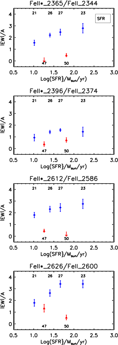
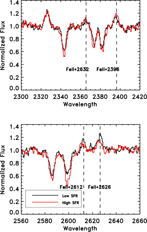
Figure 20: Left: EWs of Fe II (blue) and Fe II* lines (red) plotted as functions of SFR, numbers of objects in each subsample are shown at bottom and top. Right: Comparing co-added spectra of low SFR (black) and that of high SFR (red).

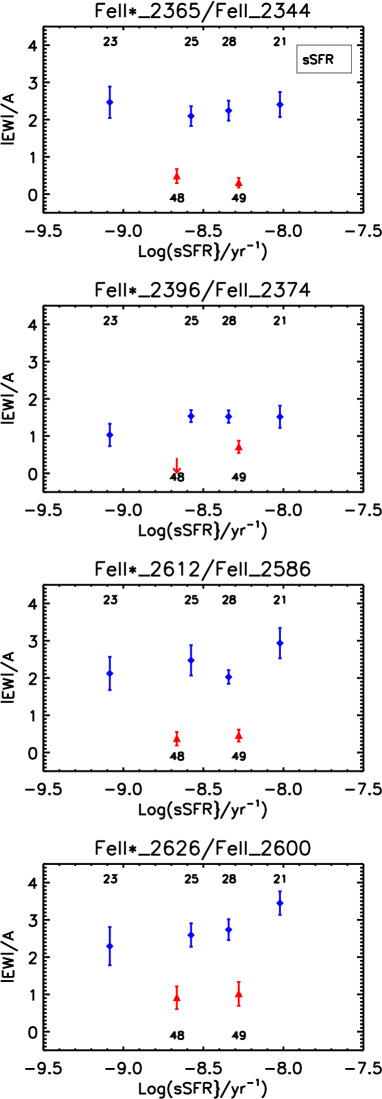
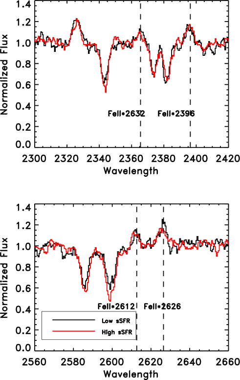
Figure 21: Left: EWs of Fe II (blue) and Fe II* lines (red) plotted as functions of sSFR, numbers of objects in each subsample are shown at bottom and top. Right: Comparing co-added spectra of lower sSFR (black) and that of higher sSFR (red).