Probing Beyond Standard Model via Hawking Radiated Gravitational Waves

Abstract

We propose a novel technique to probe the beyond standard model (BSM) of particle physics. The mass spectrum of unknown BSM particles can be scanned by observing gravitational waves (GWs) emitted by Hawking radiation of black holes. This is because information on the radiation of the BSM particles is imprinted in the spectrum of the GWs. We fully calculate the GW spectrum from evaporating black holes taking into account the greybody factor. As an observationally interesting application, we consider primordial black holes which evaporate in the very early universe. In that case, since the frequencies of GWs are substantially redshifted, the GWs emitted with the BSM energy scales become accessible by observations.

I I. Introduction

Last year, Higgs particle is discovered Aad:2012tfa and all particles in the standard model of particle physics are eventually identified. However, many phenomena which cannot be explained within the standard model have been found (e.g. dark matter, inflation, neutrino mass, etc). A number of hypothetical particles are introduced and supposed to be observed in the future. Since those beyond standard model (BSM) particles are assumed to be very heavy and/or weakly coupling to the standard model particles, to detect them is not a easy task. In fact, no evidence of a BSM particle is found in Large Hadron Collider, so far. Therefore it is very important to consider a novel technique to probe BSM particles.

In this paper, we propose a new way to scan the mass spectrum of the BSM particles by using gravitational waves (GWs) which are radiated by light black holes (BHs). It is well known that light BHs lose their masses by emitting particles through Hawking radiation and finally evaporate Page:1976df ; Hawking:1974sw . A BH emits only particles whose mass are smaller than Hawking temperature $T_{\rm BH}$,

$$M\lesssim T_{\rm BH}\equiv M_{\rm Pl}^{2}/M_{\rm BH},$$ (1)

where $M_{\rm Pl}$ is the reduced Planck mass and $M_{\rm BH}$ is the mass of the BH. $T_{\rm BH}$ increases as the BH loses its mass. Thus the BH begins to radiate a heavy particle with a mass $M_{\rm BSM}$ when the Hawking temperature reaches the mass, $T_{\rm BH}\simeq M_{\rm BSM}$. Since Hawking temperature goes up to the Planck scale right before the evaporation of a BH, any particles whose masses are less than $M_{\rm Pl}$ can be radiated by evaporating BHs.

The mass spectrum of BSM particles is imprinted in the power spectrum of GWs from evaporating BHs. Roughly speaking, this is because when a BH begins to emit a heavy particle, the number of degrees of freedom (DOF) radiated by the BH changes and the ratio between the energy going to GWs and the total radiative energy also changes. This drop of the energy fraction causes a step like feature in the GW spectrum. In eq. (2), the relationship between the BSM mass spectrum and the resultant GW spectrum is sketched,

$$\rho\left(M_{\rm BSM}\right)\rightarrow g(T_{\rm BH})\rightarrow T_{\rm BH}(t)\rightarrow\Omega_{\rm GW}(\nu_{0}).$$ (2)

The BSM mass spectrum, $\rho\left(M_{\rm BSM}\right)$, determines the DOF emitted by BHs as a function of Hawking temperature, $g(T_{\rm BH})$. The mass loss rate of a BH is proportional to it, $\partial_{t}M_{\rm BH}(t)\propto g(T_{\rm BH})$, and we can solve the time evolution of the BH mass, $M_{\rm BH}(t),$ or equivalently, that of the Hawking temperature $T_{\rm BH}(t)$. Then it is workable to compute the resultant spectrum of the GWs, $\Omega_{\rm GW}(\nu_{0})$, or any other particles. Note that the spectrum of photons or neutrinos can also be candidates for observational probe but we focus on the graviton case in this paper, because the interaction with other particles is negligible.

The imprinted feature of the BSM physics in the GW spectrum appears at the frequency which corresponds to the energy scale of the BSM. Such a high frequency GW is perhaps undetectable. However, if one identifies the BHs as primordial black holes (PBHs) PBHreview which evaporate in the very early universe, the emitted GWs are substantially redshifted and become accessible.

To obtain a proper spectrum form, we take into account the greybody factor which is often ignored but significantly alters the spectrum. Moreover, since we do not know the actual BSM theory, we assume that all the BSM particles live at the GUT scale to demonstrate a readable spectrum.

The rest of paper is organized as follows. In section 2, we briefly review Hawking radiation and greybody factor. In section 3, the spectrum of GWs emitted by a BH without cosmic expansion is calculated. In section 4, the spectrum of GWs produced by PBHs is computed and its observability is discussed. In section 5, we conclude.

II II. Hawking radiation

In this section, let us briefly review Hawking radiation and the greybody factor of gravitons. The energy spectrum of a graviton emitted by the Hawking radiation of a single BH per unit time is given by Hawking:1974sw

$$\frac{\mathrm{d}E_{\rm GW}}{\mathrm{d}t\mathrm{d}\omega}=\frac{1}{2\pi}\frac{\omega}{e^{\omega/T_{\rm BH}}-1}\times 2\Gamma(2GM_{\rm BH}\omega),$$ (3)

where $\omega$ is the energy of the graviton, $\Gamma$ denotes the greybody factor (or the absorption coefficient) and the factor 2 in front of $\Gamma$ reflects the two polarization of graviton. On the Black hole event horizon, particles are radiated with the thermal distribution (blackbody) while not all of them reach a distant observer because of the gravitational potential of the BH. The greybody factor, $\Gamma$, represent the probability that a particle with an energy $\omega$ travels to the infinite distance despite of the BH potential. The greybody factor is obtained by solving the equation of motion around the BH of the particle in interest. In the case of tensor perturbation around a Schwarzschild BH, it is written as Regge:1957td

$$\left[\frac{\mathrm{d}^{2}}{\mathrm{d}x^{2}}+\omega^{2}-V(r,l)\right]Q_{l}(r)=0,$$ (4)

$$V(r,l)=\frac{r-1}{r}\left[\frac{l(l+1)}{r^{2}}-\frac{3}{r^{3}}\right]=0,$$ (5)

where $r$ is the radial coordinate and $x$ is Tortoise coordinate, $x\equiv r+r\ln(r-1)$. Note that in this section, we set Schwarzschild radius as 1,

$$r_{s}\equiv 2GM_{\rm BH}=1.$$ (6)

Eq. (4) is called “Regge-Wheeler equation”. One can check the definition of $Q_{l}(r)$ in their paper Regge:1957td , but it is basically the $l$-mode of the graviton field whose polarization is odd. The even mode has more complicated potential while its greybody factor is identical to the odd mode Chandrasekhar:1985kt . Note that the label of the spherical harmonics should be $l\geq 2$ in the graviton case.

Since the potential $V(r,l)$ vanish at $r\to 1$ and $\infty$, the asymptotic solution of $Q_{l}$ is given by plane waves

$$Q_{l}\to e^{i\omega x}+R_{l}e^{-i\omega x}\quad(x\to-\infty;\ {\rm near\ horizon}),$$ (7)

$$Q_{l}\to T_{l}e^{i\omega x}\qquad\qquad(x\to+\infty;\ {\rm infinite\ distance}),$$ (8)

where $R_{l}$ and $T_{l}$ are the reflection, transmission coefficients, respectively. Eq. (4) has the same form as the Schrödinger equation and hence we can use the analogy with the tunneling problem in quantum mechanics. Then the greybody factor of graviton is given by

$$\Gamma(\omega)=\sum_{l=2}(2l+1)|T_{l}|^{2}.$$ (9)

The analytic expressions of $|T_{l}|^{2}$ in the low energy limit $\omega\ll 1$ and the greybody factor in the high energy limit $\omega\gg 1$ are known,

$$|T_{l}|^{2}\xrightarrow{\omega\ll 1}4\pi\left(\frac{\omega}{2}\right)^{2l+2}\left[\frac{\Gamma(l+3)\Gamma(l-1)}{\Gamma(2l+1)\Gamma(l+3/2)}\right]^{2},$$ (10)

$$\Gamma(\omega)\xrightarrow{\omega\gg 1}\frac{27}{4}\omega^{2}.$$ (11)

For general $\omega$, however, $T_{l}$ cannot be solved analytically and a numerical calculation is needed. We numerically obtain $\Gamma(\omega)$ and plot it in fig. 1. Our result is consistent with previous works MacGibbon:1991tj ; Page:1976df . Therefore by integrating eq. (3) with respect to time $t$, the GW spectrum produced by a single BH can be obtained.

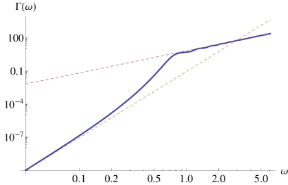
Figure 1: The blue solid line is the greybody factor of graviton introduced in eq. (3) and numerically obtained based on eq. (9)). The yellow and red dashed line represent the asymptotic behaviors in $\omega\ll 1$ (eq. 10) and $\omega\gg 1$ (eq. 11), respectively.

Before finishing this section, let us mention the effective DOF emitted by a BH. If one ignores greybody factor and consider a BH as a black-body radiator, the Stefan-Boltzmann law yields

$$\frac{\mathrm{d}E}{\mathrm{d}t}=\frac{\pi^{2}}{120}gT_{\rm BH}^{4}A_{\rm BH}=g\frac{\pi}{480}T_{\rm BH}^{2}$$ (12)

where $A_{\rm BH}\equiv 4\pi r_{s}^{2}$ is the area of the BH and $g$ denotes the number of emitted DOF. Comparing eqs. (3) and (12), Anantua et al. Anantua:2008am have introduced the following effective DOF $g_{s}$ including the effect of greybody factors:

$$\frac{\mathrm{d}E_{s}}{\mathrm{d}t}=\int^{\infty}_{0}\frac{\mathrm{d}\omega}{2\pi}\frac{\omega\Gamma_{s}(\omega)}{e^{\omega/T_{\rm BH}}-1}\equiv g_{s}\frac{\pi}{480}T_{\rm BH}^{2},$$ (13)

where $s$ is the spin of the particle in interest. The values of $g_{s}$ are given by MacGibbon:1991tj

$$g_{s=0}\approx 7.26,\quad g_{s=1/2}^{\rm uncharged}\approx 4.00,\quad g_{s=1/2}^{\rm charged}\approx 3.86,\quad$$

$$g_{s=1}\approx 1.63,\quad g_{s=2}\approx 0.185\,,$$ (14)

where “(un)charged” denotes the electric charge of the emitted spinor. One obtains the total DOF in the standard model as comment1

$$g_{\rm SM}\approx 4\times 10^{2}\,.$$ (15)

Therefore after all the standard model particles are begun to radiate, less than $0.1\%$ of the total emitted energy is radiated as gravitons. Note that this result is different by a order of magnitude from the naive estimation by the effective DOF in thermal equilibrium, $2/106.75\approx 2\%$.

III III. GW spectrum from evaporating BH

In this section, we calculate the GW spectrum produced by a single BH without cosmic expansion. For simplicity, we consider that the total effective DOF changes instantly and only once at a BSM mass scale,

$$g_{\rm tot}(T_{\rm BH})=\left\{\begin{array}[]{ll}g_{1}&\ (T_{\rm BH}<M_{{\rm BSM}})\\ g_{2}&\ (T_{\rm BH}>M_{{\rm BSM}})\end{array}\right..$$ (16)

Then solving the evolution equation of a BH mass,

$$\frac{\mathrm{d}M_{\rm BH}}{\mathrm{d}t}=-g_{\rm tot}(T_{\rm BH})\frac{\pi}{480}T_{\rm BH}^{2},$$ (17)

one can obtain the time evolution of $T_{\rm BH}$ as Fujita:2013bka

$$T_{\rm BH}(t)=\left\{\begin{array}[]{ll}T_{0}(1-\frac{t}{\tau_{1}})^{-1/3}&\,(0<t<t_{c})\\ M_{\rm BSM}(1-\frac{t-t_{c}}{\tau_{2}})^{-1/3}&\,(t_{c}<t<\tau_{\rm tot})\end{array}\right.,$$ (18)

where $T_{0}\equiv T_{\rm BH}(0)$ is the initial Hawking temperature, $\tau_{1}\equiv 160M_{\rm Pl}^{2}/\pi g_{1}T_{0}^{3}$ is the lifetime of the BH if $g_{\rm tot}=g_{1}$ regardless of $T_{\rm BH}$, $t_{c}\equiv\tau_{1}(1-T_{0}^{3}/M_{\rm BSM}^{3})$ is the time when $g_{\rm tot}$ changes, $\tau_{2}\equiv 160M_{\rm Pl}^{2}/\pi g_{2}M_{\rm BSM}^{3}$ is the lifetime after $t=t_{c}$ and $\tau_{\rm tot}\equiv t_{c}+\tau_{2}$ is the total lifetime of the BH.

Substituting eq. (18) into eq. (3), we obtain the time derivative of the graviton spectrum, $\mathrm{d}E_{\rm GW}/\mathrm{d}t\mathrm{d}\omega$, as a function of time. Nonetheless, it is important to notice that if the BSM scale $M_{\rm BSM}$ is much higher than the experimentally accessible scale, we cannot resolve the time variability of $\mathrm{d}E_{\rm GW}/\mathrm{d}t\mathrm{d}\omega$. For example, provided $M_{\rm BSM}\gg T_{0}=10^{-5}M_{\rm Pl}$ and $g_{1}=g_{\rm SM}$, the BH lifetime is $\tau_{\rm tot}\approx 10^{14}M_{\rm Pl}^{-1}\approx 3\times 10^{-29}$sec. Therefore, in practice, the BH evaporates instantaneously and the observed spectrum is the time integral of eq. (3). Then we find

$$\frac{\mathrm{d}E_{\rm GW}}{\mathrm{d}\omega} =\frac{\omega}{\pi}\int_{0}^{\tau_{\rm tot}}\mathrm{d}t\frac{\Gamma(\omega/4\pi T_{\rm BH}(t))}{e^{\omega/T_{\rm BH}(t)}-1},$$ (19)

$$=\frac{480}{\pi^{2}g_{1}}\frac{M_{\rm Pl}^{2}}{\omega^{2}}\left[\int^{\omega/T_{0}}_{\omega/M_{\rm BSM}}\mathrm{d}X\frac{X^{2}\Gamma(X/4\pi)}{e^{X}-1}\right.$$

$$\qquad\ \ \ +\left.\frac{g_{1}}{g_{2}}\int^{\omega/M_{\rm BSM}}_{0}\mathrm{d}X\frac{X^{2}\Gamma(X/4\pi)}{e^{X}-1}\right],$$ (20)

where we define $X\equiv\omega/T_{\rm BH}(t)$. The integrand in eq. (20) has a peak at $X\approx 10$ since the greybody factor $\Gamma(x)$ is suppressed for $x\lesssim 0.8$ (see fig. 1). Therefore gravitons with energy $\omega$ are mostly emitted when $\omega\approx 10T_{\rm BH}(t)$. This GW spectrum is numerically evaluated and plotted in fig. 2.

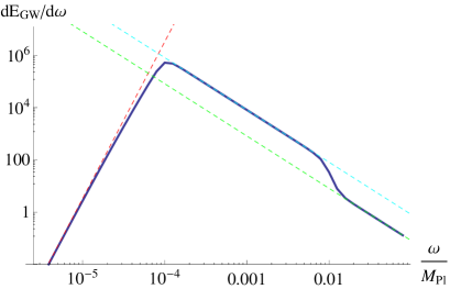
Figure 2: The blue solid line is the GW spectrum produced by a single BH (see eq. (19)). We set parameters as $T_{0}=10^{-5}M_{\rm Pl},M_{\rm BSM}=10^{-3}M_{\rm Pl}$ (GUT scale), $g_{1}=g_{\rm SM}$ and $g_{2}=10g_{\rm SM}$. The step like feature appears at $\omega\approx 10M_{\rm BSM}$ and the amplitude drops there by the factor of $g_{1}/g_{2}$. The red, cyan and green dashed lines represent the asymptotic behaviors given by eqs. (21) and (23).

Let us derive asymptotic expressions of eq. (20). For $\omega\ll T_{0}$, the first line in eq. (20) has the main contribution. Using eq. (10) with $l=2$, namely $\Gamma(x)\sim 4x^{6}/45$, and the Taylor expansion in the denominator, one can show

$$\frac{\mathrm{d}E_{\rm GW}}{\mathrm{d}\omega}\xrightarrow{\omega\ll T_{0}}\frac{\pi^{-8}}{768g_{1}}\frac{\omega^{6}M_{\rm Pl}^{2}}{T_{0}^{8}}.$$ (21)

On the other hand, for $\omega\gg T_{0}$, $\omega$ is greater than $T_{\rm BH}(t)$ at the beginning while $T_{\rm BH}(t)$ finally becomes much larger than $\omega$. Thus the integration interval can be approximated by $X=[0,\infty]$. The numerical evaluation yields

$$\int^{\infty}_{0}\mathrm{d}X\frac{X^{2}\Gamma(X/4\pi)}{e^{X}-1}\approx 0.07\,,$$ (22)

and one finds

$$\frac{\mathrm{d}E_{\rm GW}}{\mathrm{d}\omega}\xrightarrow{\omega\gg T_{0}}\frac{3.4}{g_{1,2}}\frac{M_{\rm Pl}^{2}}{\omega^{2}},$$ (23)

where $g_{1,2}$ is $g_{1}$ for $\omega\lesssim 10M_{\rm BSM}$ and $g_{2}$ for $\omega\gtrsim 10M_{\rm BSM}$. These approximated spectra, which are plotted in fig. 2 as dashed lines, clearly explain that the step like feature appears at $\omega\approx 10M_{\rm BSM}$ and the amplitude drops there by the factor of $g_{1}/g_{2}$. The reason of the drop of the amplitude can be understood that the energy ratio going to gravitons decreases as the total DOF of the Hawking radiation increases.

The GW spectrum, fig. 2, can be realized if a single BH evaporates in our neighborhood in which the cosmic expansion is negligible. Although $T_{0}$ should be taken much lower in that case, it does not affect the step like feature. Thus if we could observe such spectrum, it is possible to know the mass scale and the DOF, namely the mass spectrum, of BSM particles. Unfortunately, however, it is difficult to observe the step in this case because its frequency is around $M_{\rm BSM}$ and is probably too high to be detected even in the future.

In the next section, we consider primordial black holes (PBHs) which evaporate in very early universe. The frequency of a graviton which was emitted by a PBH gets substantially redshifted before coming to the earth and hence its frequency can be low enough to be observed.

IV IV. GW spectrum from PBH

In this section, we calculate the GW spectrum produced by PBHs. The GW spectrum from PBHs has been computed in previous works Dolgov:2011cq ; Anantua:2008am but neither the greybody factor nor the change of the DOF are taken into account (however the latter is discussed in ref. Fujita:2014hha ). In the case of PBHs, two additional effect should be considered; cosmic expansion and the number density of PBHs.

PBHs are formed at

$$t_{\rm form}\simeq(8\pi\gamma T_{0})^{-1}$$ (24)

where the initial mass of a PBH is given by $M_{0}=4\pi\gamma\rho/3H^{3}(t_{\rm form})$ and $T_{0}\equiv M_{\rm Pl}^{2}/M_{0}$. Provided that PBHs are formed at the radiation dominant era, the PBH energy fraction increases, $\Omega_{\rm BH}\equiv\rho_{\rm BH}/3M_{\rm Pl}^{2}H^{2}\propto a$. Therefore if the initial energy fraction, $\beta\equiv\Omega_{\rm BH}(t_{\rm form})$, is large enough, $\beta\gtrsim\sqrt{g_{1}}M_{\rm Pl}/36\sqrt{\gamma}M_{0}$, PBHs dominate the universe before their evaporation at $t_{\rm evap}\equiv t_{\rm form}+\tau_{\rm tot}\simeq t_{c}$. In that case, from the onset of the PBH domination until the evaporation, the universe is in matter dominant era and the total energy density at the evaporation is given by

$$\rho_{\rm evap}\simeq\frac{4M_{\rm Pl}^{2}}{3t_{c}^{2}}.$$ (25)

Ignoring the change of the DOF in the thermal bath, one finds the scale factor at the evaporation is

$$a_{\rm evap}\simeq a_{\rm eq}\left(\frac{\rho_{\rm eq}}{\rho_{\rm evap}}\right)^{1/4}\simeq\left(\frac{3a_{\rm eq}t_{c}^{2}\rho_{\rm now}}{4M_{\rm Pl}^{2}}\right)^{1/4},$$ (26)

where the subscript “eq” denotes the time of matter-radiation equality and $\rho_{\rm now}$ is the energy density at present. Using the scaling, $a\propto t^{1/2}$ during radiation dominant era and $a\propto t^{2/3}$ during matter dominant era, one can obtain the scale factor $a(t)$ from the PBH formation until the evaporation.

Remembering $\omega(t)=2\pi\nu_{0}/a(t)$ where $\nu_{0}$ is the comoving frequency, we find that $\Omega_{\rm GW}\equiv\rho_{\rm now}^{-1}\mathrm{d}\rho_{\rm GW}/\mathrm{d}\ln\nu_{0}$ of the Hawking radiated gravitons at present is written by

$$\Omega_{\rm GW}(\nu_{0})=\frac{4\pi\nu_{0}^{2}}{\rho_{\rm now}}\int^{t_{\rm evap}}_{t_{\rm form}}\mathrm{d}t\,\frac{a^{2}n_{\rm BH}\Gamma(\nu_{0}/2aT_{\rm BH})}{e^{2\pi\nu_{0}/aT_{\rm BH}}-1},$$ (27)

where $n_{\rm BH}$ is the PBH number density with the initial value, $n_{\rm BH}(t_{\rm form})=3\beta M_{\rm Pl}^{2}/4M_{0}t_{\rm form}^{2}$. We numerically evaluate this equation and plot it in fig. 3.

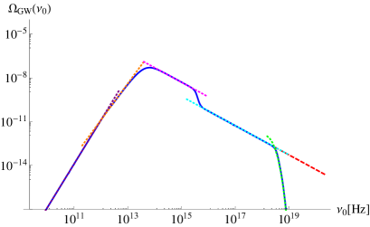
Figure 3: The blue solid line is $\Omega_{\rm GW}(\nu_{0})$ produced by evaporating PBHs (see eq. (27)). The parameters are same as fig. 2 with $\gamma=0.2$ and $\beta=10^{-4}$. The step like feature appears at $\nu_{0}\approx 10^{15}$Hz and the amplitude drops there by the factor of $g_{1}/g_{2}$. The cutoff at $\nu_{0}\approx 10^{18}$Hz is introduced by hand because the contribution from $T_{\rm BH}\geq M_{\rm Pl}$ is not reliable. The red dashed line show the case without the cutoff. The colorful dotted lines represent approximated spectra derived in appendix and confirm the validity of the numerical calculation.

Again one can see the step like feature in the GW spectrum. Furthermore, in the case of fig. 3, the frequency of the step is redshifted by the factor of $a_{\rm evap}\approx 10^{-24}$, and given by

$$\frac{2\pi\nu_{\rm step}}{a_{\rm evap}}\approx 10M_{\rm BSM}\ \Longleftrightarrow\ \nu_{\rm step}\approx 10^{15}{\rm Hz}.$$ (28)

Thus the frequency of the step is now accessible (remember $(4-8)\times 10^{14}$Hz is the frequency of visible light). In fact, the GW detector built by the group in university of Birmingham has sensitivity at $\nu_{0}\approx 10^{15}$Hz Cruise:2012zz . Although the sensitivity is not enough at present, it is expected to increase significantly in the future Li:2008qr .

It should be noted that the step frequency $\nu_{\rm step}$ depend on the initial mass of the PBHs. Here we consider that the PBHs are formed right after inflation due to the preheating Suyama:2004mz while PBHs can be formed by many other processes PBHreview . Then $M_{0}\simeq 10^{5}M_{\rm Pl}$ is obtained from the Hubble parameter right after inflation, $H_{f}\simeq 10^{13}$GeV, which is favored based on the BICEP2 result Ade:2014xna .

The Hawking radiation, eq. (3), is derived based on the quasi-classical treatment and is no longer reliable for $\omega\gtrsim M_{\rm Pl}$. Therefore we introduce the cutoff in the integral range of eq.(27) by replacing $t_{\rm evap}$ by $t_{p}\equiv t_{\rm evap}-160/\pi g_{2}M_{\rm Pl}$ at which the Hawking temperature reaches $M_{\rm Pl}$. Because of this artificial cutoff, $\Omega_{\rm GW}(\nu_{0})$ in fig.3 rapidly falls at $\nu_{\rm cut}\approx 10^{18}$Hz while the red dashed line shows the case without the cutoff.

V V. Summary and Discussion

In this paper, we demonstrate that if the DOF of Hawking radiation increases at a BSM scale, a step like feature is imprinted in the GW spectrum produced by evaporating BHs. Since the step height and the frequency of the feature indicate the number of additional DOF and the energy scale of BSM particles, respectively, we can scan the mass spectrum of the actual BSM theory by observing the GW spectrum. We assume that all BSM particles live at $10^{-3}M_{\rm Pl}$ for simplicity, set the initial mass of the PBH as $10^{5}M_{\rm Pl}$ inspired by the BICEP2 result, and calculate the GW spectrum from the PBHs (see fig. 3). It is found that the frequency of the spectrum feature is substantially redshifted due to cosmic expansion and enters the observable range.

In reality, the BSM mass spectrum may be distributed over many different energy scales. In that case, a lot of steps appear in the GW spectrum while our methodology is still useful. Note that BHs can radiate even “dark particles” which couple to the standard model sector very weakly. Therefore our technique is sensitive to these dark particles and can be complementary to particle accelerators or direct detection experiments.

VI Acknowledgements

We would like to thank Teruaki Suyama for useful discussions. This work is supported by World Premier International Research Center Initiative (WPI Initiative), MEXT, Japan. The author acknowledges JSPS Research Fellowship for Young Scientists, No.248160.

Appendix A APPENDIX: approximated analytic spectra

In this appendix, we derive the approximated analytic spectra plotted in fig. 3 as the dotted lines in order to cross-check our numerical result. Calculational procedures are almost same as eqs. (21) and (23).

A.1 1. $\omega(t_{\rm form})\ll 10T_{0}$

For this range of $\omega$, the peak contribution from $\omega\simeq 10T_{\rm BH}$ is never gained. Using the low energy approximations, $\Gamma(x)\simeq 4x^{6}/45$ and $e^{x}\simeq 1+x$, one finds

$$\Omega_{\rm GW}(\nu_{0})\simeq\frac{\nu_{0}^{7}}{360\rho_{\rm now}}\int^{t_{\rm evap}}_{t_{\rm form}}\mathrm{d}t\frac{n_{\rm BH}}{a^{3}T_{\rm BH}^{5}}.$$ (29)

Since the biggest contribution comes from $t\sim t_{\rm form}$, $T_{\rm BH}$ is approximated by $T_{0}$ and the above equation reads

$$\Omega_{\rm GW}(\nu_{0})\simeq\frac{\nu_{0}^{7}n_{{\rm BH},0}}{360\rho_{\rm now}a_{\rm form}^{3}T_{0}^{5}}\int^{t_{\rm evap}}_{t_{\rm form}}\mathrm{d}t\left(\frac{t_{\rm form}}{t}\right)^{3},$$ (30)

where $n_{{\rm BH},0}\equiv n_{\rm BH}(t_{\rm form})$ which can be rewritten as $n_{{\rm BH},0}=3M_{\rm Pl}^{3}\beta/4t_{\rm form}^{2}M_{0}$. Then we obtain

$$\Omega_{\rm GW}(\nu_{0})\simeq\frac{\pi\beta\gamma}{120}\frac{a_{\rm form}^{-3}\nu_{0}^{7}}{\rho_{\rm now}T_{0}^{3}}.$$ (31)

In fig. 3, this region of $\nu_{0}$ is too small to be plotted.

A.2 2. $\omega(t_{\rm form})\gg 10T_{0}\gg\omega(t_{c})$

In this range, $\omega$ becomes comparable to $10T_{\rm BH}$ because $\omega\ (\propto a^{-1})$ decreases while $T_{\rm BH}$ remains almost constant at $T_{0}$. Approximating $T_{\rm BH}(t)$ by $T_{0}$ and ignoring the contribution from $t>t_{c}$, one can show

$$\Omega_{\rm GW}(\nu_{0}) \simeq\frac{4\pi\nu_{0}^{2}}{\rho_{\rm now}}a_{\rm form}^{3}n_{\rm BH}(t_{\rm form})$$

$$\times\left[\frac{4\pi\nu_{0}t_{\rm form}}{a_{\rm form}^{2}T_{0}}\int^{\frac{2\pi\nu_{0}}{a_{\rm form}T_{0}}}_{\frac{2\pi\nu_{0}}{a_{\rm dom}T_{0}}}\mathrm{d}Y\frac{Y^{-2}\Gamma(Y/4\pi)}{e^{Y}-1}\right.$$

$$+ \left.3t_{c}\sqrt{\frac{\pi\nu_{0}}{2a_{\rm evap}^{3}T_{0}}}\int^{\frac{2\pi\nu_{0}}{a_{\rm dom}T_{0}}}_{\frac{2\pi\nu_{0}}{a_{\rm c}T_{0}}}\mathrm{d}Z\frac{Z^{-3/2}\Gamma(Z/4\pi)}{e^{Z}-1}\right],$$ (32)

where the subscript “dom” denotes the time when the PBHs dominate the universe. Two integrand have the peak at $Y\approx 9$ and $Z\approx 8$, and the numerical integral with the approximated interval $[0,\infty]$ yield,

$$\int^{\infty}_{0}\mathrm{d}Y\frac{Y^{-2}\Gamma(Y/4\pi)}{e^{Y}-1}\approx 1.4\times 10^{-5},$$ (33)

$$\int^{\infty}_{0}\mathrm{d}Z\frac{Z^{-3/2}\Gamma(Z/4\pi)}{e^{Z}-1}\approx 3.8\times 10^{-5}.$$ (34)

Therefore eq. (32) reads

$$\Omega_{\rm GW}(\nu_{0})\simeq 4\times 10^{-2}\frac{a_{\rm form}\gamma\beta T_{0}}{\rho_{\rm now}}\nu_{0}^{3}$$

$$~{}~{}~{}~{}~{}~{}~{}~{}~{}~{}~{}~{}~{}~{}~{}~{}~{}~{}~{}~{}~{}~{}~{}~{}~{}~{}~{}(a_{\rm dom}\gg\frac{2\pi\nu_{0}}{9T_{0}}\gg a_{\rm form}),$$ (35)

$$\Omega_{\rm GW}(\nu_{0})\simeq 2\times 10^{-3}\frac{a_{\rm form}^{3}n_{{\rm BH},0}t_{c}}{\rho_{\rm now}a_{\rm evap}^{3/2}T_{0}^{1/2}}\nu_{0}^{5/2}$$

$$~{}~{}~{}~{}~{}~{}~{}~{}~{}~{}~{}~{}~{}~{}~{}~{}~{}~{}~{}~{}~{}~{}~{}~{}~{}~{}~{}(a(t_{c})\gg\frac{2\pi\nu_{0}}{8T_{0}}\gg a_{\rm dom}).$$ (36)

They are shown as the purple and orange dotted lines in fig. 3.

A.3 3. $\omega(t_{c})\gg 10T_{0}$

For $t\gtrsim 0.1t_{c}$, the time variation of $T_{\rm BH}$ is significant while the cosmic expansion is negligible. One can show

$$\Omega_{\rm GW}(\nu_{0}) \simeq\frac{4\pi\nu_{0}^{2}}{\rho_{\rm now}}a_{\rm form}^{3}n_{{\rm BH},0}a_{\rm evap}^{-1}$$

$$\times\left[3\tau_{1}\left(\frac{a_{\rm evap}T_{0}}{2\pi\nu_{0}}\right)^{3}\int^{\frac{2\pi\nu_{0}}{a_{\rm evap}T_{0}}}_{\frac{2\pi\nu_{0}}{a_{\rm evap}M_{\rm BSM}}}\mathrm{d}X\frac{X^{2}\Gamma(X/4\pi)}{e^{X}-1}\right.$$

$$+ \left.3\tau_{2}\left(\frac{a_{\rm evap}M_{\rm BSM}}{2\pi\nu_{0}}\right)^{3}\int^{\frac{2\pi\nu_{0}}{a_{\rm evap}M_{\rm BSM}}}_{0}\mathrm{d}X\frac{X^{2}\Gamma(X/4\pi)}{e^{X}-1}\right].$$ (37)

Here, the time integral is split into the two parts because of the time dependence of $T_{\rm BH}(t)$ (see eq. (18)). Using eq. (22), we obtain

$$\Omega_{\rm GW}(\nu_{0})\simeq 10^{-2}a_{\rm form}^{3}a_{\rm evap}^{2}\frac{T_{0}^{3}n_{{\rm BH},0}\tau_{1}}{\rho_{\rm now}}\nu_{0}^{-1}$$

$$~{}~{}~{}~{}~{}~{}~{}~{}~{}~{}~{}~{}~{}~{}~{}~{}~{}~{}~{}~{}~{}~{}~{}~{}~{}~{}~{}~{}~{}(T_{0}\ll\frac{2\pi\nu_{0}}{10a_{\rm evap}}<M_{\rm BSM}),$$ (38)

$$\Omega_{\rm GW}(\nu_{0})\simeq 10^{-2}a_{\rm form}^{3}a_{\rm evap}^{2}\frac{M_{\rm BSM}^{3}n_{{\rm BH},0}\tau_{2}}{\rho_{\rm now}}\nu_{0}^{-1}$$

$$~{}~{}~{}~{}~{}~{}~{}~{}~{}~{}~{}~{}~{}~{}~{}~{}~{}~{}~{}~{}~{}~{}~{}~{}~{}~{}~{}~{}~{}(M_{\rm BSM}\ll\frac{2\pi\nu_{0}}{10a_{\rm evap}}<M_{\rm Pl}).$$ (39)

They are the magenta and cyan dotted lines in fig. 3. The ratio between two spectra is

$$\frac{\Omega_{\rm GW}(\nu_{\rm high})}{\Omega_{\rm GW}(\nu_{\rm low})}\simeq\frac{M_{\rm BSM}^{3}\tau_{2}}{T_{0}^{3}\tau_{1}}=\frac{g_{1}}{g_{2}},$$ (40)

and it reflects the change of the DOF.

A.4 4. $\omega(t_{\rm evap})\geq M_{\rm Pl}$

For the sake of completeness, let us obtain the analytic expression for $\nu_{0}>\nu_{\rm cut}$. Considering the contribution from $t\geq t_{p}$, one can find

$$\Omega_{\rm GW}(\nu_{0}) \simeq\frac{3}{2\pi^{2}}a_{\rm form}^{3}a_{\rm evap}^{2}\frac{n_{{\rm BH},0}\tau_{2}M_{\rm BSM}^{3}}{\rho_{\rm now}\nu_{0}}$$

$$\times\int^{\infty}_{\frac{2\pi\nu_{0}}{a_{\rm evap}M_{\rm Pl}}}\mathrm{d}X\frac{X^{2}\Gamma(X/4\pi)}{e^{X}-1}.$$ (41)

In this region, one see $X\gg 1$ and the high energy approximation, $\Gamma(x)\simeq 27x^{2}/4$, can be used. Then it reads

$$\Omega_{\rm GW}\simeq\frac{1620}{\pi}\frac{a_{\rm form}^{3}}{a_{\rm evap}^{2}}\frac{n_{{\rm BH},0}\nu_{0}^{3}}{g_{2}\rho_{\rm now}M_{\rm Pl}^{2}}\exp\left[-\frac{2\pi\nu_{0}}{a_{\rm evap}M_{\rm Pl}}\right].$$ (42)

It is shown as the green dotted line in fig. 3. Note that in this region, a graviton physical energy at the emission exceeds the Planck scale and no reliable treatment is established.

References

- (1) G. Aad et al. [ATLAS Collaboration], Phys. Lett. B 716, 1 (2012) S. Chatrchyan et al. [CMS Collaboration], Phys. Lett. B 716, 30 (2012)
- (2) S. W. Hawking, Commun. Math. Phys. 43, 199 (1975) [Erratum-ibid. 46, 206 (1976)];
- (3) D. N. Page, Phys. Rev. D 13, 198 (1976); D. N. Page, Phys. Rev. D 14, 3260 (1976). D. N. Page, Phys. Rev. D 16, 2402 (1977).
- (4) M.Y. Khlopov, Res. Astron. Astrophys. 10, 495 (2010); B.J. Carr, K. Kohri, Y. Sendouda, and J.’i. Yokoyama, Phys. Rev. D 81, 104019 (2010), and references therein.
- (5) T. Regge and J. A. Wheeler, Phys. Rev. 108, 1063 (1957).
- (6) S. Chandrasekhar, “The mathematical theory of black holes,” (Oxford University, New York, 1983).
- (7) J. H. MacGibbon, Phys. Rev. D 44, 376 (1991).
- (8) R. Anantua, R. Easther and J. T. Giblin, Phys. Rev. Lett. 103, 111303 (2009) [arXiv:0812.0825 [astro-ph]].
- (9) Following ref. MacGibbon:1991tj , one finds . Nevertheless, since the electric charges of the quarks are approximated by in ref. MacGibbon:1991tj , this may be underestimated by a few % level.
- (10) T. Fujita, K. Harigaya and M. Kawasaki, Phys. Rev. D 88, 123519 (2013) [arXiv:1306.6437 [astro-ph.CO]].
- (11) A. D. Dolgov and D. Ejlli, Phys. Rev. D 84, 024028 (2011) [arXiv:1105.2303 [astro-ph.CO]].
- (12) T. Fujita, M. Kawasaki, K. Harigaya and R. Matsuda, Phys. Rev. D 89, 103501 (2014)
- (13) A. M. Cruise, Class. Quant. Grav. 29, 095003 (2012).
- (14) F. Li, R. M. L. Baker, Jr., Z. Fang, G. V. Stephenson and Z. Chen, Eur. Phys. J. C 56, 407 (2008) [arXiv:0806.1989 [gr-qc]].
- (15) T. Suyama, T. Tanaka, B. Bassett and H. Kudoh, Phys. Rev. D 71, 063507 (2005) [hep-ph/0410247].
- (16) P. A. R. Ade et al. [BICEP2 Collaboration], Phys. Rev. Lett. 112, 241101 (2014) [arXiv:1403.3985 [astro-ph.CO]].