New Nonequilibrium-to-Equilibrium Dynamical Scaling and
Stretched-Exponential Critical Relaxation in Cluster Algorithms

Abstract

Nonequilibrium relaxation behaviors in the Ising model on a square lattice based on the Wolff algorithm are totally different from those based on local-update algorithms. In particular, the critical relaxation is described by the stretched-exponential decay. We propose a novel scaling procedure to connect nonequilibrium and equilibrium behaviors continuously, and find that the stretched-exponential scaling region in the Wolff algorithm is as wide as the power-law scaling region in local-update algorithms. We also find that relaxation to the spontaneous magnetization in the ordered phase is characterized by the exponential decay, not the stretched-exponential decay based on local-update algorithms.

Introduction. In Monte Carlo study of phase transitions, the critical slowing down has been a serious problem. As long as local-update algorithms are used, equilibration at the critical temperature $T_{\rm c}$ is practically impossible for fairly large systems because of a large dynamical critical exponent $z$. In order to overcome this difficulty, two kinds of approaches have been proposed. One is the cluster algorithms,[1, 2] in which global update based on a percolation theory is introduced and the exponent $z$ is considered to be greatly reduced. The other is the nonequilibrium relaxation (NER) method,[3] in which the critical relaxation in local-update algorithms is analyzed with the dynamical scaling theory[4] and equilibration is avoided.

The initial aim of the present study was to integrate the two approaches and to develop a more efficient scheme. However, when early-time relaxation in cluster algorithms at $T_{\rm c}$ is precisely investigated, we find that the standard NER method based on the dynamical scaling theory no longer holds. That is, early-time relaxation is not described by the power-law decay but by the stretched-exponential decay in cluster algorithms. The NER method has been used to estimate the exponent $z$, and the results of a study of Ising models starting from the all-up state based on cluster algorithms[5] can be compared with the present results, even though a size dependence of the relaxation time $\tau$ of the energy was observed in the former. The previously-revealed logarithmic size dependence of $\tau$, which suggests $z=0$, might be consistent with our finding, although a stretched-exponential time dependence of physical quantities was not explicitly shown previously.

The outline of the present Letter is as follows. After a brief overview of the formulation of numerical analyses, we first exhibit the stretched-exponential decay at $T_{\rm c}$. In order to confirm this nontrivial behavior, we propose a new nonequilibrium-to-equilibrium scaling analysis and compare this behavior with the established power-law decay using the Metropolis algorithm at $T_{\rm c}$. We also investigate the relaxation behavior using the Wolff algorithm below $T_{\rm c}$. The background of the stretched-exponential decay and the relation with previous studies of the dynamical critical exponent $z$ are discussed, and future tasks of the present framework are proposed.

Figure 1: Magnetization profile for a typical sweep in the Ising model on a $64,000\times 64,000$ square lattice using the Wolff algorithm at $T=2.269J/k_{\rm.B}$.

Formulation. In the present Letter, we concentrate on the two-dimensional Ising model on a square lattice. Numerical calculations are started from the all-up state using the Wolff algorithm,[2] in which a single cluster is grown from a randomly chosen site up to a maximum size and is always flipped for the Ising model. The magnetization profile for a typical Monte Carlo sweep is shown in Fig. 1, where a $64,000\times 64,000$-spin system is calculated at $T=2.269\ [J/k_{\rm B}]<T_{\rm c}=2/\log(1+\sqrt{2})\ [J/k_{\rm B}]=2.2691853\cdots[J/k_{\rm B}]$. In conventional Monte Carlo algorithms, all the spins are updated once in each Monte Carlo step (MCS), whereas only a single spin cluster is updated in each step in the Wolff algorithm. Then, the definition of a MCS in one step comparable to that in conventional algorithms is “(updated spin number) / (total spin number)”.

The ordered region is characterized by a spin cluster as large as the system size, and the bulk magnetization only originates from this cluster. Other spin clusters are much smaller and the magnetization after spatial averaging vanishes. Then, as shown in Fig. 1, the value of magnetization is almost reversed when the updated cluster is of the system size. On the other hand, the value is almost unchanged when the updated cluster is not so huge. The magnetization profile is completely governed by such a system-size cluster, and the absolute value of magnetization changes continuously. Therefore, magnetization profiles for different random-number sequences (RNSs) can be averaged in the following manner.

1. Take the absolute value $|m(t)|$ for each RNS.

2. Extract data obtained from system-size-cluster update.

3. Divide relaxation time with a small enough window $\Delta t$.

4. Average data for each time window $n\Delta t\leq t<(n+1)\Delta t$ ($n=0,1,2,\ldots$) to obtain $\langle|m(t)|\rangle$.

Figure 2: Fitting curve of average magnetization at $T=T_{\rm c}$ based on the stretched-exponential scaling form (1). Data points plotted by filled circles or crosses are not used for fitting. In the inset, the optimal number of omitted data points (from the two ends of the data sequence) is determined at the minimum residue per data $\chi^{2}/N$, as represented by the arrow.

Simulation-time scaling for the largest system. We first analyze the average magnetization $\langle|m(t)|\rangle$ for the $64,000\times 64,000$-spin system and $800$ RNS with $\Delta t=0.5$ MCS. We test various physical $2$-parameter scaling forms such as the power-law or exponential decay, and find that none of these forms can explain the present relaxation data very well. Then, it would be natural to consider $3$-parameter scaling forms, even though the use of fitting functions with many free parameters is dangerous; wide degrees of freedom may result in ambiguous fitting regardless of functional form. Taking these things into account, we test the stretched-exponential form

$$\langle|m(t)|\rangle\sim C\exp\left[-(t/\tau)^{\sigma}\right],\ 0<\sigma<1,$$ (1)

which is already established in local-update algorithms below $T_{\rm c}$,[6, 7] where $\langle|m(t)|\rangle$ converges to the spontaneous magnetization $m_{\rm s}$. Equation (1) is a special case with $m_{\rm s}=0$.

When we adopt a sufficiently long simulation time, $\langle|m(t)|\rangle$ obtained in the present framework is expected to diverge from the scaling form (1) and converge to the critical magnetization $m_{\rm c}(L)$, which vanishes as $m_{\rm c}(L)\sim L^{-\beta/\nu}$ for $L\to\infty$, with the critical exponents of spontaneous magnetization $\beta$ and correlation length $\nu$. Fitting the data with Eq. (1), we have

$$\sigma=0.342\pm 0.003,\ \tau=9.3\pm 0.3,\ C=1.43\pm 0.02.$$ (2)

The fitting curve is displayed in Fig. 2, where the data points plotted by filled circles (initial ones) or crosses (longer-time ones) are not used for fitting. Since this calculation starts from $\langle|m(t=0)|\rangle=1$, which corresponds to $C=1$ in Eq. (1), several initial data points should be omitted to obtain a better fitting curve. As explained above, longer-time data points deviate from Eq. (1) and converge to $m_{\rm c}(L)$, and therefore should also be omitted. The number of omitted data points can be optimized systematically by minimizing the residue per data $\chi^{2}/N$, as shown in the inset of Fig. 2. Since systematic or statistical errors are dominant for smaller or larger number of omitted data points, respectively, the quantity $\chi^{2}/N$ is generally expected to have a minimum in between.

Figure 3: (a) Time dependence of the average magnetization based on the Metropolis algorithm for $100\times 100$- (triangles), $200\times 200$- (squares), and $400\times 400$- (circles) spin systems in a log-log plot. Tangent of the broken line corresponds to $-\beta/(z\nu)$. (b) The scaling plot explained in the text. Data in the off-scaling region are enlarged in the inset, where the broken lines represent the power-law decay and equilibrium value and act as guides for the eyes.

New nonequilibrium-to-equilibrium dynamical scaling. The above results may be insufficient as evidence of the critical scaling form (1), because even the system with $64,000\times 64,000$ spins may not be sufficiently large and the power-law region may appear for larger system sizes. Hence, we propose a new procedure to represent nonequilibrium and equilibrium regions in a panoramic manner and show that the relaxation behavior in Fig. 2 is not a small-size effect.

This procedure is first explained in the relaxation process in the Metropolis algorithm, a representative local-update algorithm. The time dependence of the average magnetization relaxed from the all-up state is displayed in Fig. 3(a) on a log-log scale for $100\times 100$-, $200\times 200$-, and $400\times 400$-spin systems represented by triangles, squares, and circles, respectively. Each data point is obtained from 6,400 RNS, where the number of RNS remains unchanged while the system size increases, because the fluctuating nonequilibrium region expands simultaneously. The power-law behavior $\langle m(t)\rangle\sim t^{-\beta/(z\nu)}$ is clearly observed even in such a small system as for the standard NER analysis. Namely, the tangent of the broken line is $-\beta/(z\nu)$, with the exact exponent $\beta/\nu=1/8$ and the dynamical exponent $z\approx 2.13$ evaluated from these data.

In order to put all the data on a single curve, the size dependence of $\langle m(t)\rangle$ in equilibrium should be cancelled by multiplying $L^{\beta/\nu}$. Since this factor violates the size independence of data in the power-law region, the simulation time should be multiplied by $L^{-z}$ for compensation, i.e. $(tL^{-z})^{-\beta/(z\nu)}=t^{-\beta/(z\nu)}L^{\beta/\nu}$. Then, we have a new scaling plot as shown in Fig. 3(b), where the tangent of the scaled data in the power-law region is the same as that in Fig. 3(a) as visualized by the broken line, and the scaled data in equilibrium fall on a horizontal line. It is interesting that the data between these two regions are also scaled on a single curve, and that such an intermediate region is quite narrow, as emphasized in the inset.

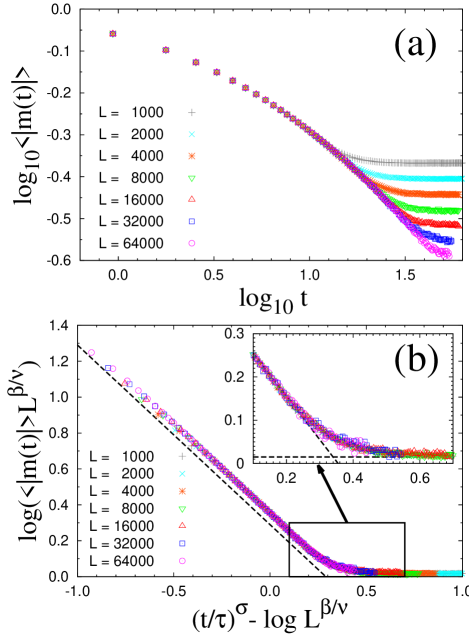
Figure 4: (Color online) (a) Time dependence of the average magnetization based on the Wolff algorithm for $1,000\times 1,000$- (crosses), $2,000\times 2,000$- (X-marks), $4,000\times 4,000$- (stars), $8,000\times 8,000$- (reverse-triangles), $16,000\times 16,000$- (triangles), $32,000\times 32,000$- (squares), and $64,000\times 64,000$- (circles) spin systems on a log-log scale. (b) Scaling plot explained in the text. The tangent of the broken line is $-1$. Data in the off-scaling region are enlarged in the inset, where the broken lines represent the stretched-exponential decay and equilibrium value and act as guides for the eyes.

Next, the average magnetization based on the Wolff algorithm for various system sizes is analyzed similarly. In Fig. 4(a), the data for $1,000\times 1,000$- (409,600 RNS), $2,000\times 2,000$- (102,400 RNS), $4000\times 4000$- (51,200 RNS), $8,000\times 8,000$- (12,800 RNS), $16,000\times 16,000$- (6,400 RNS), $32,000\times 32,000$- (1,600 RNS), and $64,000\times 64,000$- (800 RNS) spin systems are displayed on a log-log scale to enable comparison with Fig. 3(a). Apparently, the data do not exhibit a power-law decay, and the equilibration time is much shorter.

The scaling plot corresponding to Fig. 3(b) can be derived as follows: (i) Multiply $L^{\beta/\nu}$ with $\langle|m(t)|\rangle$, because the equilibrium state does not depend on the relaxation process. (ii) In accordance with Eq. (1), $\exp[-(t/\tau)^{\sigma}]$ should be replaced by $\exp[-(t/\tau)^{\sigma}]L^{\beta/\nu}$ for compensation, or by $(t/\tau)^{\sigma}\rightarrow(t/\tau)^{\sigma}-\log L^{\beta/\nu}$, as displayed in Fig. 4(b) with the estimates given in Eq. (2). Data for a wide range of system sizes are scaled well with the parameters obtained from the largest system. In this case, the off-scaling region is also quite narrow, as shown in the inset, which strongly suggests that no intermediate (i.e. power-law) region would exist between the stretched-exponential and equilibrium regions.

Figure 5: Time dependence of the average magnetization using the Wolff algorithm at $T=2.269J/k_{\rm B}$, which is slightly below $T_{\rm c}$, for $16,000\times 16,000$- (triangles), $32,000\times 32,000$- (squares), and $64,000\times 64,000$- (circles) spin systems. Convergence to the exact spontaneous magnetization $m_{\rm s}$ is almost independent of system size, and the average magnetization subtracted by $m_{\rm s}$ decays exponentially, as shown in the inset (almost-linear semilog plot).

Relaxation behavior slightly below $T_{\rm c}$. Finally, results in the ordered phase are briefly reported. In simulations based on local-update algorithms, the stretched-exponential decay with $\sigma=1/2$ was confirmed[8, 9] in the Ising model on a square lattice. Then, similar calculations based on the Wolff algorithm are performed at $T=2.269J/k_{\rm B}$, which is slightly below $T_{\rm c}$ and the same as that in Fig. 1. The average magnetization is plotted versus simulation time for $16,000\times 16,000$- (800 RNS), $32,000\times 32,000$- (100 RNS), and $64,000\times 64,000$- (100 RNS) spin systems in Fig. 5. These data rapidly converge to the exact value of the spontaneous magnetization $m_{\rm s}$, and the size dependence is negligible in this figure. In the inset, the average magnetization subtracted by $m_{\rm s}$ is plotted versus simulation time on a semilog scale. All the data fall on a straight line, that is, this quantity decays exponentially.

Discussion. In the stretched-exponential decay in the Ising model below $T_{\rm c}$ based on local-update algorithms, the exponent is expressed as $\sigma=(d-1)/2$ with the spatial dimension $d$ in terms of the droplet picture,[6] and a similar analytic relation is also expected in the present case. According to our preliminary calculations for the Ising model on a cubic lattice at $T_{\rm c}$ based on the Wolff algorithm, the stretched-exponential decay with the exponent $\sigma\approx 0.45\sim 0.5$ is observed. Our estimate for $d=2$ in Eq. (2) and this value for $d=3$ might be consistent with $\sigma=(d-1)/(d+1)$,[7] which was originally proposed for the region below $T_{c}$ but was not consistent with numerical studies.[8, 9] Further investigations are still necessary.

The scaling plot in Figs. 3(b) and 4(b) reveals that each axis of the plot is scale-invariant. That is, Fig. 3(b) shows that the simulation time in local-update algorithms is scaled as $t\sim L^{z}$ at $T=T_{\rm c}$. Similarly, Fig. 4(b) indicates that the simulation time in cluster algorithms is scaled as $t\sim(\log L)^{1/\sigma}$ at $T=T_{\rm c}$.

Studies of the dynamical critical exponent $z$ in cluster algorithms based on the equilibrium autocorrelation function of various quantities have a long history. Swendsen and Wang[1] and Wolff[10] already made such calculations using their own algorithms and obtained $z$ much smaller than that obtained with local-update algorithms. That is, the autocorrelation function in a finite system of linear size $L$ decays exponentially with the correlation time $\tau(L)$, and the exponent $z$ is evaluated from the power-law scaling $\tau(L)\propto L^{z}$. Several studies followed along this line,[11, 12, 13, 14, 15] and it was found to be difficult to distinguish between the weak power-law and logarithmic size dependences of $\tau(L)$.[13, 14] Such a logarithmic scaling means $z=0$, namely, the breakdown of standard dynamical critical behaviors.

Then, NER was introduced to investigate larger systems. Gündüc et al.[16] studied NER from the completely disordered state in the SW and Wolff algorithms, and reported $z=0$ in both cases. Du et al.[5] studied much larger systems, and found that NER from the completely ordered state gave $z=0$ for the SW and Wolff algorithms, whereas NER from the completely disordered state resulted in $z=0$ for the SW algorithm and $z\approx 1.19$ for the Wolff algorithm. Recently, Liu et al.[17] studied $z$ for the SW and Wolff algorithms using the Kibble-Zurek ansatz,[18, 19, 20] which is a kind of scaling theory based on the annealing process from a disordered state to $T_{\rm c}$. Critical exponents can be directly obtained from the size dependence of $\langle m^{2}(L)\rangle$, and they gave a small but finite $z$ comparable to that derived using equilibrium autocorrelation functions.

In a word, the exponent $z$ in cluster algorithms is not yet established even today. Although our results in this Letter appear to be consistent with Ref. 5, we do not intend to claim $z=0$. Rather, we consider that the stretched-exponential decay from the perfectly ordered state is a specific property of cluster algorithms, and that this property would be useful when $z$ is still large even in cluster algorithms. Once the scaling form is established, NER analyses similar to the power-law case can be constructed.

Summary and future tasks. We have investigated early-time nonequilibrium relaxation behaviors based on the Wolff algorithm numerically in the two-dimensional Ising model on a square lattice, and found that they are totally different from those based on local-update algorithms. That is, the average magnetization decays in a stretched-exponential law at the critical temperature $T_{\rm c}$ and in an exponential law below $T_{\rm c}$ in cluster algorithms, whereas it decays in a power law at $T_{\rm c}$ and in a stretched-exponential law below $T_{\rm c}$ in local-update algorithms. We have proposed a new scaling procedure to draw nonequilibrium and equilibrium data for various system sizes on a single curve, and found that this scheme holds well for the power-law decay in the Metropolis algorithm and the stretched-exponential decay in the Wolff algorithm. Crossover regions between the scaling and equilibrium regions appear narrow in both cases, which suggests the absence of an intermediate region.

There are many future tasks within the present framework. First, a scheme comparable to the standard NER method should be established. A procedure for evaluating $T_{\rm c}$ should be obtained, and a formalism for evaluating critical exponents without equilibrium data is required. Second, the formalism should be generalized for the first-order or BKT phase transitions. Third, essential applications for the present framework should be specified. For example, relaxation in random spin systems is too slow to evaluate by the standard NER method based on local-update algorithms, but the present approach based on cluster algorithms might be effective.

Finally, extension to the quantum Monte Carlo (QMC) method is promising. Although modern QMC algorithms based on the continuous imaginary-time formalism[21] have naturally been coupled with the cluster-update scheme,[22] NER analyses so far have been based on the world-line local update[23] or on a special algorithm with cluster update only in imaginary time[24] in order to retain the power-law decay. The present scheme enables NER analyses of QMC algorithms with cluster update, the code for which is faster and simpler than previous ones.

Investigations along these lines are now in progress.

Acknowledgement. Y. N. would like to thank Y. Tomita for stimulating discussion. He also thanks M. Kohno, S. Todo and Y. Ozeki for helpful comments. The random-number generator MT19937[25] was used for numerical calculations.

References

- [1] R. H. Swendsen and J.-S. Wang, Phys. Rev. Lett. 58, 86 (1987).
- [2] U. Wolff, Phys. Rev. Lett. 62, 361 (1989).
- [3] As a recent review, Y. Ozeki and N. Ito, J. Phys. A 40, R149 (2007).
- [4] M. Suzuki, Phys. Lett. A 58, 435 (1976), Prog. Theor. Phys. 58, 1142 (1977).
- [5] J. Du, B. Zheng, and J.-S. Wang, J. Stat. Mech. (2006), P05004.
- [6] D. A. Huse and D. S. Fisher, Phys. Rev. B 35, 6841 (1987). See also C. Tang, H. Nakanishi, and J. S. Langer, Phys. Rev. A 40, 995 (1989).
- [7] H. Takano, H. Nakanishi, and S. Miyashita, Phys. Rev. B 37, 3716 (1988).
- [8] N. Ito, Physica A 192, 604 (1993), 196, 591 (1993).
- [9] P. Grassberger and D. Stauffer, Physica A 232, 171 (1996); D. Stauffer, Physica A 244, 344 (1997).
- [10] U. Wolff, Nucl. Phys. B 322, 759 (1989).
- [11] W. Klein, T. Ray, and P, Tamayo, Phys. Rev. Lett. 62, 163 (1989).
- [12] P. Tamayo, R. C. Brower, and W. Klein, J. Stat. Phys. 58, 1083 (1990).
- [13] D. W. Heermann and A. N. Burkitt, Physica A 162, 210 (1990).
- [14] C. F. Baillie and P. D. Coddington, Phys. Rev. B 43, 10617 (1991).
- [15] P. D. Coddington and C. F. Baillie, Phys. Rev. Lett. 68, 962 (1992).
- [16] S. Gündüç, M. Dilaver, M. Aydin, and Y. Gündüç, Comp. Phys. Commun. 166, 1 (2005).
- [17] C.-W. Liu, A. Polkovnikov, and A. W. Sandvik, Phys. Rev. B 89, 054307 (2014).
- [18] T. W. B. Kibble, J. Phys. A: Math. Gen. 9, 1387 (1976).
- [19] W. H. Zurek, Nature 317, 505 (1985).
- [20] A. Chandran, A. Erez, S. S. Gubser, and S. L. Sondhi, Phys. Rev. B 86, 064304 (2012).
- [21] B. B. Beard and U.-J. Wiese, Phys. Rev. Lett. 77, 5130 (1996).
- [22] H. G. Evertz, G. Lana, and M. Marcu, Phys. Rev. Lett. 70, 875 (1993).
- [23] Y. Nonomura, J. Phys, Soc. Jpn. 67, 5 (1998), J. Phys. A : Math. Gen. 31, 7939 (1998).
- [24] T. Nakamura and Y. Ito, J. Phys. Soc. Jpn. 72, 2405 (2003).
- [25] M. Matsumoto and T. Nishimura, ACM TOMACS 8, 3 (1998). Further information is available from the Mersenne Twister Home Page, currently maintained by M. Matsumoto.