Multiscale Empirical Interpolation for Solving Nonlinear PDEs using Generalized Multiscale Finite Element Methods

Abstract

In this paper, we propose a multiscale empirical interpolation method for solving nonlinear multiscale partial differential equations. The proposed method combines empirical interpolation techniques and local multiscale methods, such as the Generalized Multiscale Finite Element Method (GMsFEM). To solve nonlinear equations, the GMsFEM is used to represent the solution on a coarse grid with multiscale basis functions computed offline. Computing the GMsFEM solution involves calculating the residuals on the fine grid. We use empirical interpolation concepts to evaluate the residuals and the Jacobians of the multiscale system with a computational cost which is proportional to the coarse scale problem rather than the fully-resolved fine scale one. Empirical interpolation methods use basis functions and an inexpensive inversion which are computed in the offline stage for finding the coefficients in the expansion based on a limited number of nonlinear function evaluations. The proposed multiscale empirical interpolation techniques: (1) divide computing the nonlinear function into coarse regions; (2) evaluate contributions of nonlinear functions in each coarse region taking advantage of a reduced-order representation of the solution; and (3) introduce multiscale proper-orthogonal-decomposition techniques to find appropriate interpolation vectors. We demonstrate the effectiveness of the proposed methods on several examples of nonlinear multiscale PDEs that are solved with Newton’s methods and fully-implicit time marching schemes. Our numerical results show that the proposed methods provide a robust framework for solving nonlinear multiscale PDEs on a coarse grid with bounded error.

1 Introduction

Solving nonlinear Partial Differential Equations (PDEs) with multiple scales and/or high-contrast in media properties is computationally expensive because of the disparity between scales that need to be represented and the inherent nonlinearities. For this reason, coarse-grid computational models are often used. These include Galerkin multiscale finite elements [3, 8, 10, 15, 16, 17, 22], mixed multiscale finite element methods [1, 2, 4, 25], the multiscale finite volume method [26], mortar multiscale methods [5, 27], and variational multiscale methods [24]. The coarse-grid models for nonlinear PDEs can be divided into several classes. One of them includes constructing nonlinear operators that allow downscaling from coarse-grid functions to fine-grid functions [18, 19]. Other types of approaches involve designing linear multiscale basis functions (which are constructed using nonlinear PDEs) on the coarse grid and using these basis functions for approximating the solution [11].

One of the challenges in these coarse-grid models is evaluating nonlinear functionals for computing the residual and the Jacobian of the operator. Some of the widely used techniques are based on Empirical Interpolation Methods (EIM) [6, 7, 9]. In the offline stage, the response of the nonlinear function is evaluated to yield solution snapshots and interpolation vectors are constructed using the Proper Orthogonal Decomposition (POD). Evaluating a few components of the nonlinear function allows performing rapid evaluation of the nonlinear function in the online stage with sufficient accuracy [7]. This procedure allows for rapid evaluations of the nonlinear function’s response in the online stage. When solving multiscale equations, these empirical interpolation techniques can be expensive because of the large problem sizes. In this paper, we design an efficient multiscale empirical interpolation framework.

Our proposed empirical interpolation techniques are based on multiscale finite element approximations that are often used for solving multiscale problems on coarse grids. The main idea of these methods is to construct local multiscale basis functions for approximating the solution over each coarse patch. Constructing these basis functions uses offline coarse-grid spaces. These spaces are constructed via judicious choices of snapshot spaces and local spectral problems that are motivated by the analysis [11]. The main objective of this paper is to design efficient local multiscale empirical interpolations that can be used in conjunction with Generalized Multiscale Finite Element Method (GMsFEM) to solve nonlinear multiscale problems with a computational cost proportional to the number of coarse-scale degrees of freedom rather than the fully resolved mesh.

When GMsFEM is used for nonlinear problems, we evaluate the residual and Jacobian in each Newton iteration which require fine-grid calculations and incur a high computational cost. We use POD-based empirical interpolation and follow the Discrete Empirical Interpolation Method (DEIM) introduced in [7]. For this reason, we refer to our method as multiscale DEIM. The main ingredients of the proposed multiscale DEIM are:

• The evaluation of the nonlinear functions is performed on the subregions associated with those of the local multiscale basis functions and the global coupling of these local representations is performed.

• In each subregion, an empirical interpolation is used as a representation of the nonlinear function which is computed based on a small dimensional multiscale representation of the solution space.

• For multiscale high-contrast problems, interpolation vectors are computed using appropriate spectral problems which involve local multiscale basis functions and ensure convergence of the method. This modified spectral problems are constructed using bounds provided by the numerical analysis of the system.

In this paper, we investigate these issues and show that one can design efficient empirical interpolation techniques in conjunction with GMsFEM. We provide error estimates and the derivations of new spectral problems for computing empirical interpolation vectors.

Representative numerical results are presented in the paper. We consider three examples: (1) nonlinear function evaluations using GMsFEM basis functions; (2) steady-state multiscale elliptic equation with nonlinear forcing; and (3) nonlinear multiscale parabolic equations with nonlinear diffusion coefficients. In all examples, we show that, by using a multiscale empirical interpolation, we can obtain an accurate solution approximation at a cost that scales with the coarse-grid size and is independent of the fine-grid size. In particular, a few interpolation modes are needed in all these examples.

The paper is organized as follows. In Section 2, we discuss empirical interpolation methods and local multiscale techniques. In Section 3, we introduce a multiscale empirical interpolation and discuss its convergence. In Section 4, applications of the multiscale empirical interpolation techniques to nonlinear PDEs are studied. In this section, we discuss GMsFEM and the use of multiscale interpolation techniques in Newton methods. Numerical results are presented in Section 5.

2 Review of basic concepts

2.1 Discrete Empirical interpolation method

In this paper, we use the Discrete Empirical Interpolation Method (DEIM) [7] for the local approximation of nonlinear functions though other empirical interpolation methods can also be used [6]. DEIM approximates a nonlinear function by means of an interpolatory projection of a few selected global snapshots of the function. The idea is to represent a function over the domain while using empirical snapshots and information in some locations (or components).

We briefly review DEIM following [7]. First, we give some motivation for using DEIM. Let ${f}(\tau)\in\mathbb{R}^{n}$ denote a nonlinear function, where $\tau$ refers to any control parameter. In a reduced-order modeling, the state vector $\tau$ is typically assumed to have a reduced-order representation, i.e., $\tau\in\mathbb{R}^{\widehat{n}}$ can be represented by fewer basis vectors, $\zeta_{1}$,…, $\zeta_{l}$, where $l\ll\widehat{n}$. Here, in general, $\widehat{n}$ can be different from $n$, though we can assume $\widehat{n}=n$. The reduced-order representation of $\tau$ usually leads us to look for a reduced-order representation of the nonlinear functions $f(\tau)$. The procedure of finding the reduced-order representation of $f(\tau)$ consists of two steps. In the first step, we would like to find $m$ basis vectors (where $m$ is much smaller than $n$), $\psi_{1}$,…, $\psi_{m}$, such that $f(\tau)$ can be approximated in the space spanned by these vectors. The error of this approximation is given by POD error which represents approximation of all possible $f(\tau_{i})$’s in the space spanned by $\psi_{1}$,…, $\psi_{m}$ [7]. In the second step, we identify a reduced-dimensional linear system that allows finding the representation of $f(\tau)$ in the space without involving $n$ operations. In this step, we typically identify $m$ equations that allow finding the coordinates of $f(\tau)$ in the space spanned by $\psi_{1}$,…, $\psi_{m}$.

We assume an approximation of the function ${f}$ obtained by projecting it into a subspace spanned by the basis functions (snapshots) $\Psi=(\psi_{{}_{1}},\cdots,\psi_{{}_{m}})\in\mathbb{R}^{n\times m}$ which are obtained by forward simulations. We write

$${f}(\tau)\approx\Psi{d}(\tau).$$ (1)

To compute the coefficient vector $d$, we select $m$ rows of (1) and invert a reduced system to compute $d(\tau)$. This can be formalized using the matrix P

$$\mbox{P}=[{e}_{\wp_{1}},\cdots,{e}_{\wp_{m}}]\in\mathbb{R}^{n\times m},$$

where ${e}_{\wp_{i}}=[0,\cdots,0,1,0,\cdots,0]^{T}\in\mathbb{R}^{n}$ is the $\wp_{i}^{\mbox{th}}$ column of the identity matrix $\mbox{I}_{n}\in\mathbb{R}^{n\times n}$ for $i=1,\cdots,m$. Multiplying Equation (1) by ${P}^{T}$ and assuming that the matrix $\mbox{P}^{T}\Psi$ is nonsingular, we obtain

$${f}(\tau)\approx\Psi d(\tau)=\Psi(\mbox{P}^{T}\Psi)^{-1}\mbox{P}^{T}{f}(\tau).$$ (2)

To summarize, approximating the nonlinear function ${f}(\tau)$, as given by Equation (2), requires the following:

• computing the projection basis $\Psi=(\psi_{{}_{1}},\cdots,\psi_{{}_{m}}).$

• identifying the indices $\{\wp_{1},\cdots,\wp_{m}\}.$

To determine the projection basis $\Psi=(\psi_{{}_{1}},\cdots,\psi_{{}_{m}})$, we collect function evaluations in an $n\times n_{s}$ matrix $\mbox{F}=[{f}(\tau_{1}),\cdots,{f}(\tau_{n_{s}})]$ and employ the POD technique to select the most energetic modes. This selection uses the eigenvalue decomposition of the square matrix $\mbox{F}^{T}\mbox{F}$ and selects the important modes using the dominant eigenvalues. These modes are used as the projection basis in the approximation given by Equation (1). In Equation (2), the term $\Psi(\mbox{P}^{T}\Psi)^{-1}\in\mathbb{R}^{n\times m}$ is computed once and stored. The $d(\tau)$ is computed using the values of the function $f(\tau)$ at $m$ points with the indices $\wp_{1},\cdots,\wp_{m}$ (identified using the DEIM algorithm). The computational saving is due to fewer evaluations of $f(\tau)$. We refer to [7] for further details.

Remark 1 (Inclusion of a priori multiscale information on the POD selection procedure).

In this paper, we explore ways to include the information about heterogeneities in the POD selection process. POD selects the dominant eigenpairs of $(\mbox{F}^{T}\mbox{F})z_{i}=\lambda_{i}z_{i}$, where $z_{i}$ are coordinates in the space $\text{Span}\{{f}(\tau_{1}),\cdots,{f}(\tau_{n_{s}})\}$. In multiscale high-contrast problems, one needs to take into account the heterogeneities when calculating the POD modes. Depending on the application in mind and on a priori information on the space of functions $u$ for which $f(u)$ needs to be computed, it is possible to improve the approximation using different inner products, say, represented by $M_{1}$ and $M_{2}$, and perform a spectral selection based on the eigenvalues of the modified eigenvalue problem $\mbox{F}^{T}M_{1}\mbox{F}=\lambda\mbox{F}^{T}M_{2}\mbox{F}z$.

2.2 Local multiscale interpolation

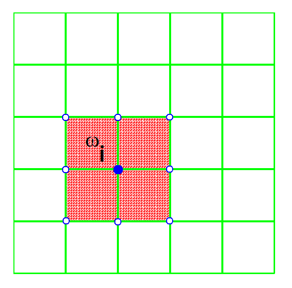
Figure 1: A coarse-grid decomposition of a two-dimensional square domain. We highlight the $i$-th coarse-node (blue circle), its neighborhood $\omega_{i}$ and all other coarse nodes in $\omega_{i}$ (white circles). The fine-mesh is depicted only for coarse-grid blocks forming the highlighted support $\omega_{i}$ of the $i$-th coarse basis.

In multiscale problems, one needs to construct local approximations of the solution using appropriately designed multiscale basis functions. We use GMsFEM, a general local multiscale strategy [11]. These methods construct local multiscale basis functions to approximate the solution over each coarse patch. Constructing these basis functions uses local offline spaces. These spaces are constructed via judicious choices of snapshot spaces and local spectral problems that are motivated by the analysis. Local multiscale basis functions are defined on a coarse grid where each coarse-grid block is a union of fine-grid blocks (see Figure 1 for a schematic representation of the coarse and fine grids).

Next, we discuss the coarse-grid projection operators without going into details. A detailed construction is presented in Section 4.2. Assume that the fine-scale problem has $n_{f}$ degrees of freedom and that the coarse-scale problem has $n_{c}$ degrees of freedom. We design a matrix $\Phi$ of size $n_{f}\times n_{c}$ whose transpose $\Phi^{T}$ of size $n_{c}\times n_{f}$ maps the fine-grid vectors to vectors of coarse degrees of freedom (coarse vectors). We refer to $\Phi$ as downscaling (or coarse-to-fine) operator and to $\Phi^{T}$ as upscaling (or fine-to-coarse projection) operator. This construction depends on several ingredients, such as the snapshot space and the eigenvalues of the offline and online problems (see Section 4.2 for details).

Locality is key to the design of the new class of DEIM techniques proposed herein. Each column of $\Phi$ is a multiscale basis function supported locally on a coarse region (see Figure 2 for an example of a basis in a coarse region). One usually has several multiscale basis functions per coarse-grid block. In the design of our multiscale DEIM, we identify multiscale basis functions (columns of $\Phi$) which have support in $\omega_{i}$. Only these selected multiscale basis functions are used in obtaining the local DEIM approximation of $f(u)$.

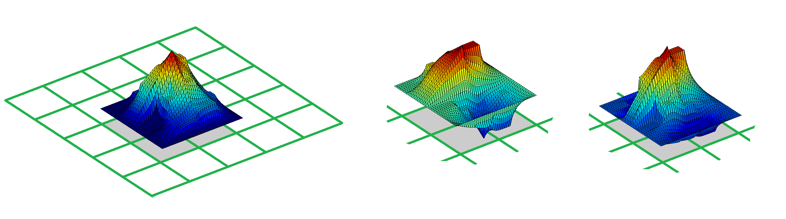
Figure 2: Illustration of three basis functions supported in the highlighted neighborhood.

When solving nonlinear PDEs, one writes the residual on the fine grid as

$$R(u)=0,$$ (3)

where $R(u)$ is the residual of nonlinear PDE and $u$ is the fine-grid solution. For instance, in a nonlinear flow problem we may have a nonlinear partial differential equation (in strong form) given by $R(u)=\alpha(x){\partial u\over\partial t}-\mbox{div}\big{(}\kappa(x,u,\mu_{\kappa})\,\nabla u\big{)}-g(u,x,\mu)$; see Sections 4.3 and 5 for further details and examples. Here, both $u$ and $R(u)$ are $n$-dimensional vectors defined on a fine grid. Using the projection operator $\Phi$, we project (3) onto the coarse degrees of freedom (noting that $\Phi z$ is an approximation of the fine-grid solution, that is, $u\approx\Phi z$)

$$\Phi^{T}R(\Phi z)=0.$$ (4)

This equation is formulated on the coarse degrees of freedom constructed on the coarse-grid; however, computing the residual $R(\Phi z)$ requires fine-grid evaluations. Moreover, computing the Jacobians for each Newton iteration, defined as

$$J(z)=\nabla_{z}R(\Phi z),$$

also requires fine-grid evaluations. Here, our main goal is to use the multiscale DEIM to compute $R(\Phi z)$ and $J(z)$ efficiently. In particular, using the multiscale DEIM approximation similar to (1), we can write

$$R(\Phi z)\approx\Psi d(z).$$

Consequently, the residual computation involves

$$\Phi^{T}\Psi d(z),$$ (5)

which can be efficiently computed by pre-computing $\Phi^{T}\Psi$. A similar procedure can be applied to compute the Jacobian $J(z)$.

3 Multiscale Discrete Empirical Interpolation Methods

3.1 Algorithm

We detail the multiscale Discrete Empirical Interpolation Methods (multiscale DEIM). A key idea is that, instead of solving the fine-grid problem (3), we solve the coarse problem (4). An important issue in the solution of the coarse problem (4) is the evaluation of the nonlinear terms. In order to fix ideas, in this paper we consider scalar problems and the evaluation of the nonlinear terms of the from $f(u)$ where (the fine-grid finite element function) $u:D\to\mathbb{R}$ and $f:\mathbb{R}\to\mathbb{R}$. In our approach we use the DEIM procedure to efficiently evaluate the nonlinear terms. We stress the following main observations that are explored and ultimately motivate the design of the multiscale DEIM procedure presented below.

• In applications to multiscale PDEs (where one solves (4) instead of the fine-grid problem (3)) the nonlinear functional $f$ needs to be evaluated with vectors of the form $u=\Phi z$ that are the downscaling of solutions obtained by reduced-order models. Thus, $f(\Phi z)$ needs to be computed in the span of coarse-grid snapshot vectors which has a reduced dimension.

• Due to the fact that multiscale basis functions are supported on a coarse-grid neighborhood, it is sufficient to obtain the DEIM approximation in each coarse-node neighborhood.

• More elaborate spectral selections may be needed to identify the elements of empirical interpolation vectors such that the resulting multiscale DEIM approximation is accurate in adequate norms that depend on physical parameters such as the contrast and small scales.

We recall that each column of $\Phi$ is the vector representation of a (fine grid) finite element function with local support so we can identify columns of $\Phi$ with locally supported basis functions. Let us introduce the notation $I^{\omega_{i}}$ which represents the set of indexes of coarse basis functions (which correspond to the columns of $\Phi$) such that these basis functions have support on $\omega_{i}$ (see Figures 1 and 2). Furthermore, we introduce partition of unity diagonal matrices defined on $\omega_{i}$ denoted by $\mathcal{D}_{i}$ and such that

$$\sum_{i}\mathcal{D}_{i}=\mbox{I}_{n},$$ (6)

where $\mbox{I}_{n}$ is the identity matrix of size $n\times n$. Here, for each node $i$, the $\mathcal{D}_{i}$ is a diagonal matrix with the main diagonal that consists of a partition of unity vector $\chi_{i}$, i.e., $\mathcal{D}_{i}=\chi_{i}(x_{j})\delta_{ji}$, where $x_{j}$ are nodal points and $\delta_{ji}$ is the Kronecker symbol.

We note that $f(u)$ can be written as

$$f(u)=\sum_{i}\mathcal{D}_{i}f(u).$$

Observe that $\mathcal{D}_{i}f(u)$ is defined only on the fine-grid nodes of $\omega_{i}$. Since $f:\mathbb{R}\to\mathbb{R}$, and thus only a few basis functions (with indices from $I^{\omega_{i}}$ ) contribute to it since for $u=Rz=\sum_{j=1}^{n_{c}}z_{j}\phi_{j}$ and $x\in\omega_{i}$ we have $u(x)=\sum_{j\in I^{\omega_{i}}}z_{j}\phi_{j}(x)$. Thus, we have that

$$f(\Phi z)=\sum_{i}\mathcal{D}_{i}f(\Phi z)=\sum_{i}\mathcal{D}_{i}f(\sum_{j\in I^{\omega_{i}}}z_{j}\phi_{j}),$$

where $\phi_{j}$ are basis vectors ($j$-th columns of $\Phi$).

Next, in each neighborhood $\omega_{i}$, we can perform an empirical interpolation locally since we can write

$$\sum_{i}\mathcal{D}_{i}f(\sum_{j\in I^{\omega_{i}}}z_{j}\phi_{j})=\sum_{i}\mathcal{D}_{i}f^{\omega_{i}}(\sum_{j\in I^{\omega_{i}}}z_{j}\phi_{j}^{\omega_{i}})=\sum_{i}\mathcal{D}_{i}f^{\omega_{i}}(\Phi^{\omega_{i}}z^{\omega_{i}}),$$

where $f^{\omega_{i}}$ is the restriction of $f$ to $\omega_{i}$, $\phi_{j}^{\omega_{i}}$ are the components of $\phi_{j}$ in $\omega_{i}$, $\Phi^{\omega_{i}}$ is the matrix with columns $\phi_{j}^{\omega_{i}}$, and $z^{\omega_{i}}$ represents a vector containing only entries $z_{j}$ with $j\in I^{\omega_{i}}$. Therefore, noting that $f^{\omega_{i}}$ depends on a few $z$’s, we perform an empirical interpolation using DEIM. For each coarse region $\omega_{i}$ we apply DEIM as introduced in Section 2.1 to construct an approximation of the type (1) for the function $\tau\mapsto f^{\omega_{i}}(\Phi^{\omega_{i}}\tau)$ with $\tau=z^{\omega_{i}}$. According to (1) we obtain $\Psi^{\omega_{i}}$ and $d^{\omega_{i}}$ such that the following approximation holds,

$$f^{\omega_{i}}(\sum_{j\in I^{\omega_{i}}}z_{j}\phi_{j}^{\omega_{i}})\approx\widetilde{f}^{\omega_{i}}(\sum_{j\in I^{\omega_{i}}}z_{j}\phi_{j}^{\omega_{i}}):=\Psi^{\omega_{i}}d^{\omega_{i}}(z^{\omega_{i}}).$$ (7)

With this empirical interpolation, we have

$$f(\Phi z)\approx\widetilde{f}(\Phi z):=\sum_{i}\mathcal{D}_{i}\widetilde{f}^{\omega_{i}}(\sum_{j\in I^{\omega_{i}}}z_{j}\phi_{j}^{\omega_{i}})=\sum_{i}\mathcal{D}_{i}\Psi^{\omega_{i}}d^{\omega_{i}}(z^{\omega_{i}}).$$ (8)

In simulation, $\mathcal{D}_{i}\Psi^{\omega_{i}}$ can be pre-computed and thus approximating $f(\Phi z)$ can be done at a lower cost.

DEIM Algorithm	Multiscale Discrete Empirical Interpolation Method
Input:	Coarse grid, partition of unity matrices $\mathcal{D}_{i}$, multiscale basis matrix $\Phi^{\omega_{i}}$,
	a projection basis matrix $\Psi^{\omega_{i}}$ obtained by applying POD on a sequence of
	$n_{s}$ function evaluations
	For each $\omega_{i}$
	1. Set $[\mid\rho\mid,\wp_{1}^{\omega_{i}}]=\max\{\mid\psi_{{}_{1}}^{\omega_{i}}\mid\}$
	2. Set $\Psi^{\omega_{i}}=(\psi_{{}_{1}}^{\omega_{i}})$, $\mbox{P}=({e}_{\rho_{1}})$, , and $\overrightarrow{\wp}^{\omega_{i}}=(\wp_{1}^{\omega_{i}})$
	3. for $\ell=2,\cdots,m$ do
	Solve $((\mbox{P}^{\omega_{i}})^{T}\Psi^{\omega_{i}}){d}^{\omega_{i}}=(\mbox{P}^{\omega_{i}})^{T}\psi_{{}_{\ell}}^{\omega_{i}}$
	Compute ${r}=\psi_{{}_{\ell}}^{\omega_{i}}-\Psi^{\omega_{i}}{d}^{\omega_{i}}$
	Compute $[\mid\rho\mid,\wp_{\ell}^{\omega_{i}}]=\max\{\mid{r}\mid\}$
	Set $\Psi^{\omega_{i}}=(\Psi^{\omega_{i}}\;\psi_{{}_{\ell}}^{\omega_{i}})$, $\mbox{P}^{\omega_{i}}=(\mbox{P}^{\omega_{i}}\;{e}_{\rho_{\ell}^{\omega_{i}}})$, and $\wp^{\omega_{i}}=\left(\begin{array}[]{c}\wp^{\omega_{i}}\\ \wp_{\ell}^{\omega_{i}}\\ \end{array}\right)$
	end for
	$d^{\omega_{i}}=((P^{\omega_{i}})^{T}\Psi^{\omega_{i}})^{-1}\Psi^{\omega_{i}}$
Output:	the interpolation indices $\overrightarrow{\wp}^{\omega_{i}}=(\wp_{1}^{\omega_{i}},\cdots,\wp_{m}^{\omega_{i}})^{T}$ and
	$f(\Phi z)\approx\sum_{i}\mathcal{D}_{i}\Psi^{\omega_{i}}d^{\omega_{i}}(z^{\omega_{i}})$

Table 1: Multiscale Discrete Empirical Interpolation Method.

The algorithm for multiscale DEIM, used to compute the approximation in (7) for each coarse region, is presented in Table 1.

3.2 Analysis

In the rest of the section, we present the analysis of the multiscale DEIM designed above. In order to simplify the expressions, we use the notation $A\preceq B$ to signify that there is a constant $C$ such that $A\preceq CB$, where this constant $C$ is independent of the vectors involved and of dimension $n$.

We start by using the definition of $\widetilde{f}(\Phi z)$ in (8) to get,

$$\|f(\Phi z)-\widetilde{f}(\Phi z)\|^{2} = \|\sum_{i}\mathcal{D}_{i}f(\Phi z)-\widetilde{f}(\Phi z)\|^{2}$$ (9)

$$= \|\sum_{i}\mathcal{D}_{i}(f(\Phi z)-\widetilde{f}^{\omega_{i}}(\Phi^{\omega_{i}}z^{\omega_{i}}))\|^{2}$$

$$\preceq \sum_{i}\|f(\Phi^{\omega_{i}}z^{\omega_{i}})-\widetilde{f}^{\omega_{i}}(\Phi^{\omega_{i}}z^{\omega_{i}})\|^{2}$$

$$= \sum_{i}\|f^{\omega_{i}}(\Phi^{\omega_{i}}z^{\omega_{i}})-\Psi^{\omega_{i}}d^{\omega_{i}}(z^{\omega_{i}})\|_{\omega_{i}}^{2}.$$

Here, we have applied a triangle inequality and the fact that the entries of the diagonal matrices $\mathcal{D}_{i}$ are less than one. The hidden constant is the maximum number of coarse nodes in $I^{\omega_{i}}$, that is, $\max_{i}\#(I^{\omega_{i}})$, where $\#$ is the cardinality of the set. This number is finite, is independent of the fine-grid parameter $n$ and depends only on the coarse triangulation configuration.

Following DEIM estimates in [7] (see Lemma 3.2.), we can write

$$\|f^{\omega_{i}}(\Phi^{\omega_{i}}z^{\omega_{i}})-\Psi^{\omega_{i}}d^{\omega_{i}}(z^{\omega_{i}})\|_{\omega_{i}}^{2}\leq\|((P^{\omega_{i}})^{T}\Psi^{\omega_{i}})^{-1}\|^{2}\|f^{\omega_{i}}-\mathcal{P}_{\Psi^{\omega_{i}}}f^{\omega_{i}}\|_{\omega_{i}}^{2}.$$ (10)

Here $((P^{\omega_{i}})^{T}\Psi^{\omega_{i}})^{-1}$ is assumed invertible and $\|f^{\omega_{i}}-\mathcal{P}_{\Psi^{\omega_{i}}}f^{\omega_{i}}\|_{\omega_{i}}^{2}$ is the projection of the error onto the space spanned by $\Psi^{\omega_{i}}$ (where $\mathcal{P}_{\Psi^{\omega_{i}}}$ is the orthogonal projection in the vector norm $\|\cdot\|_{\omega_{i}}$ to the space spanned by $\Psi^{\omega_{i}}$ ).

To estimate $\|f^{\omega_{i}}-\mathcal{P}_{\Psi^{\omega_{i}}}f^{\omega_{i}}\|_{\omega_{i}}^{2}$, we can consider an error estimate that is typical for POD estimates. The error over all snapshots is given by

$$\sum_{j=1}^{n^{\omega_{i}}}\|f^{\omega_{i},j}-\mathcal{P}_{\Psi^{\omega_{i}}}f^{\omega_{i},j}\|_{\omega_{i}}^{2}=\sum_{j=L_{i}+1}^{n^{\omega_{i}}}\lambda^{\omega_{i}}_{j},$$

where ${n^{\omega_{i}}}$ are the number of snapshots in the region $\omega_{i}$: $\{f^{\omega_{i},j}\}_{j=1}^{n^{\omega_{i}}}$. The $\lambda^{\omega_{i}}_{j}$ are eigenvalues (in the decreasing order) of $\Psi^{\omega_{i}}(\Psi^{\omega_{i}})^{T}$, and $L_{i}$ is the number of selected eigenvalues whose corresponding eigenvectors are used in the empirical interpolation. This estimate requires that the snapshots used in the above estimate appear in the local POD. One can also show that, for an arbitrary element $f^{\omega_{i}}$ in the span of snapshots, we have

$$\|f^{\omega_{i}}-\mathcal{P}_{\Psi^{\omega_{i}}}f^{\omega_{i}}\|_{\omega_{i}}^{2}\preceq\lambda^{\omega_{i}}_{L_{i}+1}\|f^{\omega_{i}}\|_{\omega_{i}}^{2}.$$

With this latter estimate, we can write

$$\sum_{i}\|f^{\omega_{i}}(\Phi^{\omega_{i}}z^{\omega_{i}})-\Psi^{\omega_{i}}d^{\omega_{i}}(z^{\omega_{i}})\|_{\omega_{i}}^{2} \preceq \sum_{i}\|((P^{\omega_{i}})^{T}\Psi^{\omega_{i}})^{-1}\|^{2}\|f^{\omega_{i}}-\mathcal{P}_{\Psi^{\omega_{i}}}f^{\omega_{i}}\|_{\omega_{i}}^{2}$$ (11)

$$\preceq \sum_{i}\|((P^{\omega_{i}})^{T}\Psi^{\omega_{i}})^{-1}\|^{2}\|f^{\omega_{i}}-\mathcal{P}_{\Psi^{\omega_{i}}}f^{\omega_{i}}\|_{\omega_{i}}^{2}$$

$$\preceq \sum_{i}\|((P^{\omega_{i}})^{T}\Psi^{\omega_{i}})^{-1}\|^{2}\lambda^{\omega_{i}}_{L_{i}+1}\|f^{\omega_{i}}\|_{\omega_{i}}^{2}.$$

By inserting (11) into (9), we obtain the estimate

$$\|f(\Phi z)-\widetilde{f}(\Phi z)\|^{2}=\max_{i}\{\|((P^{\omega_{i}})^{T}\Psi^{\omega_{i}})^{-1}\|^{2}\lambda^{\omega_{i}}_{L_{i}+1}\}\|f\|^{2}.$$ (12)

One may need a special inner product for multiscale high-contrast equations to ensure an appropriate bound, as discussed in Section 4.4.

4 Applications to multiscale PDEs

In this section, we describe the offline-online computational procedure that is used to solve the forward problem on a coarse grid. We elaborate on possible choices for the associated bilinear forms to be used in the coarse space construction. Below we offer a general outline of the multiscale procedure. For details on the constructions and further considerations we refer to [11, 14, 12, 13].

• Offline computations:

  • 1.0. Coarse grid generation.

  • 1.1. Construction of snapshot space used to compute the offline space.

  • 1.2. Construction of a small dimensional offline space by dimensional reduction in the space of local snapshots.

• Online computations:

  • 2.1. For each input parameter set, compute multiscale basis functions.

  • 2.2. Solution of a coarse-grid problem for given forcing term and boundary conditions.

4.1 Problem setup

We consider various non-linear elliptic equations of the form

$$\alpha(x){\partial u\over\partial t}-\mbox{div}\big{(}\kappa(x,u,\mu_{\kappa})\,\nabla u\big{)}=g(u,x,\mu)\,\,\text{in}\,D,$$ (13)

where $u=0$ on $\partial D$. Performing multiscale simulations requires appropriate local multiscale basis functions. We discuss this procedure next. The procedure below identifies local basis functions. Denoting these basis functions by $\phi_{j}$, we seek the solution

$$u(x,t_{n})=\sum_{i}z_{i}^{n}\phi_{i}$$ (14)

that solves (13). We employ an implicit time discretization and use the Newton method to solve the resulting nonlinear system at each time level. In this case, the residual form of problem (13) can be written as

$$R_{m}(z^{n+1}) =\sum_{j}(z_{j}^{n+1}-z_{j}^{n})\int_{D}\alpha(x)\phi_{j}\phi_{m}$$

$$+\sum z_{j}^{n+1}\int_{D}\kappa(x,\sum_{l}z_{l}^{n+1}\phi_{l},\mu_{\kappa})\nabla\phi_{j}\nabla\phi_{m}$$

$$-\int_{D}g(\sum_{l}z_{l}^{n+1}\phi_{l},x,\mu)=0,$$ (15)

where $z^{n}$ is the solution at the previous time step and $z^{n+1}$ is the value of the solution at the latest iteration level.

4.2 Multiscale spatial discretization via GMsFEM

In the offline computation, we first construct a snapshot space $V_{\text{snap}}^{\omega_{i}}$. Constructing the snapshot space may involve solving various local problems for different choices of input parameters or different fine-grid representations of the solution in each coarse region. We denote each snapshot vector (listing the solution at each node in the domain) using a single index and create the following matrix

$$\Phi_{\text{snap}}=\left[\phi_{1}^{\text{snap}},\ldots,\phi_{M_{\text{snap}}}^{\text{snap}}\right],$$

where $\phi_{j}^{\text{snap}}$ denotes the snapshots and $M_{\text{snap}}$ denotes the total number of functions to keep in the local snapshot matrix construction.

In order to construct an offline space $V_{\text{off}}$, we perform a dimension reduction process in the space of snapshots using an auxiliary spectral decomposition. The main objective is to use the offline space to efficiently (and accurately) construct a set of multiscale basis functions to be used in the online stage. More precisely, we seek for a subspace of the snapshot space such that it can approximate any element of the snapshot space in the appropriate sense which is defined via auxiliary bilinear forms. At the offline stage the bilinear forms are chosen to be parameter-independent, such that there is no need to reconstruct the offline space for each $\nu$ value, where $\nu$ is assumed to be a parameter that represents $u$ and $\mu_{\kappa}$ in $\kappa(x,u,\mu_{\kappa})$. For constructing the offline space, we use the average of over the coarse region $\omega_{i}$ in $\kappa(x,\nu)$. Thus, $\nu$ represents both the average of $u$ and $\mu$. We consider the following eigenvalue problem in the space of snapshots:

$$A^{\text{off}}\Phi_{k}^{\text{off}} = \lambda_{k}^{\text{off}}S^{\text{off}}\Phi_{k}^{\text{off}},$$ (16)

where

$$\displaystyle A^{\text{off}} =[a^{\text{off}}_{mn}]=\int_{\omega_{i}}\overline{\kappa}(x,\nu)\nabla\phi_{m}^{\text{snap}}\cdot\nabla\phi_{n}^{\text{snap}}=\Phi_{\text{snap}}^{T}\overline{A}\Phi_{\text{snap}},$$ (17)

$$\displaystyle S^{\text{off}} =[s^{\text{off}}_{mn}]=\int_{\omega_{i}}\widetilde{\overline{\kappa}}(x,\nu)\phi_{m}^{\text{snap}}\phi_{n}^{\text{snap}}=\Phi_{\text{snap}}^{T}\overline{S}\Phi_{\text{snap}}.$$ (18)

In the definitions of $A^{\text{off}}$ and $S^{\text{off}}$ above, the coefficient $\overline{\kappa}(x,\nu)$ is defined as a parameter-averaged coefficient. The coefficient $\widetilde{\overline{\kappa}}(x,\nu)$ can be chosen simply as $\widetilde{\overline{\kappa}}(x,\nu)=\overline{\kappa}(x,\nu)$ or in more sophisticated manners that include information about multiscale finite element basis functions; we refer to [11] for details and examples. In Equation (17), $\overline{A}$ (similarly for $\overline{S}$ in (18)) denotes a fine-scale matrix, except that parameter-averaged coefficients are used in its construction, and also that $\overline{A}$ is constructed by integrating only on $\omega_{i}$. To generate the offline space, we then choose the smallest $M_{\text{off}}$ eigenvalues from Equation (16) and form the corresponding eigenvectors in the respective space of snapshots by setting $\phi_{k}^{\text{off}}=\sum_{j}\Phi_{kj}^{\text{off}}\phi_{j}^{\text{snap}}$ (for $k=1,\ldots,M_{\text{off}}$), where $\Phi_{kj}^{\text{off}}$ are the coordinates of the vector $\Phi_{k}^{\text{off}}$. See [11, 15] for further details. We then create the offline matrices

$$\Phi_{\text{off}}=\left[\phi_{1}^{\text{off}},\ldots,\phi_{M_{\text{off}}}^{\text{off}}\right]$$

to be used in the online space construction.

The online coarse space is used within the finite element framework to solve the original global problem, where continuous Galerkin multiscale basis functions are used to compute the global solution. In particular, we seek a subspace of the respective offline space such that it can approximate well any element of the offline space in an appropriate metric. At the online stage, the bilinear forms are chosen to be parameter-dependent. The following eigenvalue problems are posed in the offline space:

$$A^{\text{on}}(\nu)\Phi_{k}^{\text{on}} = \lambda_{k}^{\text{on}}S^{\text{on}}(\nu)\Phi_{k}^{\text{on}},$$ (19)

where

$$\displaystyle A^{\text{on}}(\nu) =[a^{\text{on}}(\nu)_{mn}]=\int_{\omega_{i}}\kappa(x,\nu)\nabla\phi_{m}^{\text{off}}\cdot\nabla\phi_{n}^{\text{off}}=\Phi_{\text{off}}^{T}A(\nu)\Phi_{\text{off}},$$

$$\displaystyle S^{\text{on}} =[s^{\text{on}}_{mn}]=\int_{\omega_{i}}\widetilde{{\kappa}}(x,\nu)\phi_{m}^{\text{off}}\phi_{n}^{\text{off}}=\Phi_{\text{off}}^{T}{S}(\nu)\Phi_{\text{off}},$$

and $\kappa(x,\nu)$ and $\widetilde{{\kappa}}(x,\nu)$ are now parameter dependent. As before, the coefficient $\widetilde{{\kappa}}(x,\nu)$ can be chosen simply as $\widetilde{{\kappa}}(x,\nu)={\kappa}(x,\nu)$ or can include the multiscale finite element basis functions. The choice of $\widetilde{\kappa}$ has implications on the dimensions of the resulting coarse spaces; see [11]. To generate the online space, we then choose the smallest $M_{\text{on}}$ eigenvalues from (19) and form the corresponding eigenvectors in the offline space by setting $\phi_{k}^{\text{on}}=\sum_{j}\Phi_{kj}^{\text{on}}\phi_{j}^{\text{off}}$ (for $k=1,\ldots,M_{\text{on}}$), where $\Phi_{kj}^{\text{on}}$ are the coordinates of the vector $\Phi_{k}^{\text{on}}$. If $\kappa(x,u)=k_{0}(x)b(u)$, then one can use the parameter-independent case of GMsFEM. In this case, there is no need to construct the online space (or the online space is the same as the offline space). From now on, we denote the online space basis functions by $\phi_{i}$.

4.3 Newton method and Newton-DEIM

We consider a time-dependent nonlinear flow governed by the following parabolic partial differential equation

$$\frac{\partial u}{\partial t}-\mbox{div}\big{(}\kappa(x,u,\mu)\,\nabla u\big{)}=h(x)\,\,\text{in}\,D.$$ (20)

The finite element discretization of Equation (20) yields a system of ordinary differential equations given by

$$\mbox{M}\dot{\mbox{U}}+\mbox{F}(\mbox{U})=\mbox{H},$$ (21)

where

$$\mbox{U}=\left(\begin{array}[]{cccc}u_{1}&u_{2}&\cdots&u_{n_{f}}\\ \end{array}\right)^{T}$$

is the vector collecting the pressure values at the fine-scale nodes with $n_{f}$ being the total number of fine-scale nodes and H is the right-hand-side vector obtained by discretization. In our derivations and simulations, we assume that

$$\kappa(x,u,\mu)=\sum_{q=1}^{Q}\kappa_{q}(x)b_{q}(u,\mu)$$ (22)

for some $Q$. In general, $\kappa(x,u,\mu)$, can be approximated as in (22) using the offline basis functions (see [6, 11] for dealing with the nonlinearity in $u$ within each coarse region). This results in

$$\mbox{F}(\mbox{U},\mu)=\sum_{q=1}^{Q}\mbox{A}_{q}\Lambda_{1}^{q}(\mbox{U},\mu)\mbox{U},$$

where we have

$$\mbox{A}_{ij}^{q} =\int_{D}\kappa_{q}\nabla\phi^{0}_{i}\cdot\nabla\phi^{0}_{j},\;\;\;\mbox{M}_{ij}=\int_{D}\phi^{0}_{i}\phi^{0}_{j}\;,\;\;\;\mbox{H}_{i}=\int_{D}\phi^{0}_{i}h\;,$$

$$\Lambda_{1}^{q}(\mbox{U},\mu) =\mbox{diag}\left(\begin{array}[]{cccc}b_{q}(u_{1},\mu)&b_{q}(u_{2},\mu)&\cdots&b_{q}(u_{N_{f}},\mu)\\ \end{array}\right),$$

and $\phi^{0}_{i}$ are piecewise linear basis functions defined on a fine triangulation of $D$.

Employing the backward Euler scheme for the time marching process, we obtain

$$\mbox{U}^{n+1}+\Delta t\;\mbox{M}^{-1}\mbox{F}(\mbox{U}^{n+1})=\mbox{U}^{n}+\Delta t\;\mbox{M}^{-1}\mbox{H},$$ (23)

where $\Delta t$ is the time-step size and the superscript $n$ refers to the temporal level of the solution. We let

$$\mbox{R}(\mbox{U}^{n+1})=\mbox{U}^{n+1}-\mbox{U}^{n}+\Delta t\;\mbox{M}^{-1}\mbox{F}(\mbox{U}^{n+1})-\Delta t\;\mbox{M}^{-1}\mbox{H}$$ (24)

with derivative

$$\mbox{J}(\mbox{U}^{n+1})=D\mbox{R}(\mbox{U}^{n+1}) =I+\Delta t\;\mbox{M}^{-1}D\mbox{F}(\mbox{U}^{n+1})$$

$$=I+\sum_{q=1}^{Q}\Delta t\;\mbox{M}^{-1}\mbox{A}_{q}\Lambda_{1}^{q}(\mbox{U}^{n+1})+\sum_{q=1}^{Q}\Delta t\;\mbox{M}^{-1}\mbox{A}_{q}\Lambda_{2}^{q}(\mbox{U}^{n+1}),$$ (25)

where

$$\Lambda_{2}^{q}(\mbox{U},\mu)=\mbox{diag}\left(\begin{array}[]{cccc}\frac{\partial b_{q}(u_{1},\mu)}{\partial u}&\frac{\partial b_{q}(u_{2},\mu)}{\partial u}&\cdots&\frac{\partial b_{q}(u_{N_{f}},\mu)}{\partial u}\end{array}\right),$$

and $D$ is the multi-variate gradient operator defined as $D\mbox{R}(\mbox{U})=\partial\mbox{R}_{i}/\partial\mbox{U}_{j}$. The scheme involves, at each time step, the following iterations

$$\mbox{J}(\mbox{U}^{n+1}_{(k)})\Delta\mbox{U}^{n+1}_{(k)} =-\Big{(}\mbox{U}^{n+1}_{(k)}-\mbox{U}^{n}+\Delta t\;\mbox{M}^{-1}\mbox{F}(\mbox{U}^{n+1}_{(k)})-\Delta t\;\mbox{M}^{-1}\mbox{H}\Big{)}$$

$$\mbox{U}^{n+1}_{(k+1)} =\mbox{U}^{n+1}_{(k)}+\Delta\mbox{U}^{n+1}_{(k)},$$

where the initial guess is $\mbox{U}^{n+1}_{(0)}=\mbox{U}^{n}$ and $k$ is the iteration counter. The above iterations are repeatedly applied until $\parallel\Delta\mbox{U}^{n+1}_{(k)}\parallel$ is less than a specific tolerance.

In our simulations, we use $Q=1$ (see (22)) for the definition of $Q$) as our focus is on localized multiscale interpolation of nonlinear functionals that arise in discretization of multiscale PDEs. With this choice, we do not need to compute the online multiscale space (i.e., the online space is the same as the offline space).

We use the solution expansion given by Equation (14) and employ the multiscale framework to obtain a set of $n_{c}$ ordinary differential equations that constitute a reduced-order model; that is,

$$\dot{z}=-(\Phi^{T}\mbox{M}\Phi)^{-1}\Phi^{T}\mbox{F}(\Phi z)+(\Phi^{T}\mbox{M}\Phi)^{-1}\Phi^{T}\mbox{H}.$$ (26)

Thus, the original problem with $n_{f}$ degrees of freedom is reduced to a dynamical system with $n_{c}$ dimensions where $n_{c}\ll n_{f}$.

The nonlinear term $(\Phi^{T}\mbox{M}\Phi)^{-1}\Phi^{T}\mbox{F}(\Phi z)$ in the reduced-order model, given by Equation (26), has a computational complexity that depends on the dimension of the full system $n_{f}$. This nonlinear term requires matrix multiplications and full evaluation of the nonlinear function F at the $n_{f}$-dimensional vector $\Phi z(t)$. As such, solving the reduced system still requires extensive computational resources and time. To reduce this computational requirement, we use multiscale DEIM as described in the previous section. In this case, computational savings can be obtained in a forward run of the nonlinear model.

To solve the reduced system, we employ the backward Euler scheme; that is,

$$z^{n+1}+\Delta t\;\widetilde{\mbox{M}}^{-1}\widetilde{\mbox{F}}(z^{n+1})=z^{n}+\Delta t\;\widetilde{\mbox{M}}^{-1}\widetilde{\mbox{H}},$$ (27)

where $\widetilde{\mbox{M}}=\Phi^{T}\mbox{M}\Phi$, $\widetilde{\mbox{F}}(z)=\Phi^{T}\mbox{F}(\Phi z)$, and $\widetilde{\mbox{H}}=\Phi^{T}\mbox{H}$. We let

$$\widetilde{\mbox{R}}(z^{n+1})=z^{n+1}-z^{n}+\Delta t\;\widetilde{\mbox{M}}^{-1}\widetilde{\mbox{F}}(z^{n+1})-\Delta t\;\widetilde{\mbox{M}}^{-1}\widetilde{\mbox{H}}$$ (28)

with derivative

$$\widetilde{\mbox{J}}(z^{n+1})=D\widetilde{\mbox{R}}(z^{n+1}) =I+\Delta t\;\widetilde{\mbox{M}}^{-1}D\widetilde{\mbox{F}}(z^{n+1})$$

$$=I+\sum_{q=1}^{Q}\Delta t\;\widetilde{\mbox{M}}^{-1}\Phi^{T}\mbox{A}_{q}\Lambda_{1}^{q}(\Phi z^{n+1})\Phi+\sum_{q=1}^{Q}\Delta t\;\widetilde{\mbox{M}}^{-1}\Phi^{T}\mbox{A}_{q}\Lambda_{2}^{q}(\Phi z^{n+1})\Phi.$$

The scheme involves, at each time step, the following iterations

$$\widetilde{\mbox{J}}(z^{n+1}_{(k)})\Delta z^{n+1}_{(k)} =-\Big{(}z^{n+1}_{(k)}-z^{n}+\Delta t\;\widetilde{\mbox{M}}^{-1}\widetilde{\mbox{F}}(z^{n+1}_{(k)})-\Delta t\;\widetilde{\mbox{M}}^{-1}\widetilde{\mbox{H}}\Big{)}$$ (29)

$$z^{n+1}_{(k+1)} =z^{n+1}_{(k)}+\Delta z^{n+1}_{(k)},$$ (30)

where the initial guess is $z^{n+1}_{(0)}=z^{n}$. The above iterations are repeated until $\parallel\Delta z^{n+1}_{(k)}\parallel$ is less than a specific tolerance. We use multiscale DEIM as detailed in Section 3 to approximate the nonlinear functions that appear in the residual $\widetilde{\mbox{R}}$ and the Jacobian $\widetilde{\mbox{J}}$ and, therefore, reduce the number of function evaluations.

4.4 The use of multiscale POD for DEIM

When designing empirical interpolation methods for high-contrast problems, it is important to take into account heterogeneities and perform an interpolation using special weighted norms. These norms are derived based on the analysis discussed next.

Consider the approximation of

$$\sum_{i}c_{i}\int_{D}\kappa(x)b(\sum_{l}z_{l}\phi_{l})\nabla\phi_{i}\nabla\phi_{j}$$ (31)

that appears in the residual function (28). For multiscale DEIM, we split this integral using partition of unity matrices as discussed earlier in (6) and re-write it for the discretization of the stiffness matrix. We introduce the partition of unity $\{\chi^{\omega_{k}}\}$ subordinated to the coarse regions $\{\omega_{k}\}$. The relation with the partition of unity matrices $\mathcal{D}_{k}$ is that the action of $\mathcal{D}_{k}$ is the multiplication of the corresponding finite element function by the partition of unity function $\chi^{\omega_{k}}$. We obtain,

$$\sum_{i}c_{i}\int_{D}\kappa(x)b(\sum_{l}z_{l}\phi_{l})\nabla\phi_{i}\nabla\phi_{j} =\sum_{i,k}c_{i}\int_{\omega_{k}}\chi^{\omega_{k}}(x)\kappa(x)b\left(\sum_{l}z_{l}\phi_{l}^{\omega_{k}}\right)\nabla\phi_{i}^{\omega_{k}}\nabla\phi_{j}^{\omega_{k}}$$

$$=\sum_{i,k}c_{i}\int_{\omega_{k}}\chi^{\omega_{k}}(x)\kappa(x)b\left(\sum_{l\in I^{\omega_{k}}}z_{l}\phi_{l}^{\omega_{k}}\right)\nabla\phi_{i}^{\omega_{k}}\nabla\phi_{j}^{\omega_{k}}.$$ (32)

The interpolation for $b(\sum_{l\in I^{\omega_{k}}}z_{l}\phi_{l}^{\omega_{k}})$ is performed in the region $\omega_{k}$. Each term in the sum (4.4) can be written as

$$\int_{\omega_{k}}m_{ij}^{\omega_{k}}(x)b(\sum_{l\in I^{\omega_{k}}}z_{l}\phi_{l}^{\omega_{k}}),$$ (33)

where $m_{ij}^{\omega_{k}}(x)=\chi^{\omega_{k}}(x)\kappa(x)\nabla\phi_{i}^{\omega_{k}}\nabla\phi_{j}^{\omega_{k}}$.

To evaluate (33), one needs to take into account the weight $m_{ij}^{\omega_{k}}(x)$ for high-contrast multiscale problems, where $m_{ij}^{\omega_{k}}(x)$ can have very high values in some subregions within $\omega_{k}$. Otherwise, the accuracy of the method substantially deteriorates. However, the weighting function is not uniquely defined and depends on particular basis functions that are involved in the integration. We propose the use of a weight function that is computed by summing over all indices $i,j$ (which provides an upper bound for every $m_{ij}^{\omega_{k}}(x)$) and using only a few dominant modes. For high-contrast problems, $m_{ij}^{\omega_{k}}(x)$ is very high in the regions of high conductivity and this high value can be estimated using only the first basis function. We propose using

$$\widetilde{m}^{\omega_{k}}=\sum_{i}\kappa(x)|\nabla\phi_{1}^{\omega_{i}}|^{2}$$

which is defined in the entire domain. Here, $\phi_{1}^{\omega_{k}}$ is the first basis function (associated to the first dominant mode in the online GMsFEM selection procedure). One can also use additional basis functions to construct the weight $\widetilde{m}^{\omega_{k}}$. For implementing this procedure, we need to define $\Psi^{\omega_{i}}$ in (7) using weighted POD modes. This can simply be done using the matrix corresponding to the mass matrix $\widetilde{m}^{\omega_{k}}$ as $M_{1}$ in Remark 1 ($M_{2}$ is the identity matrix of appropriate size).

Using the above argument, one can write the error in the residuals of multiscale DEIM $\widetilde{R}^{D}$ and $R(z)$.

$$\begin{split}R(z)-\widetilde{R}^{D}(z)=\sum_{i,k}c_{i}\int_{\omega_{k}}\chi^{\omega_{k}}(x)\kappa(x)(b(\sum_{l\in I^{\omega_{k}}}z_{l}\phi_{l}^{\omega_{k}})-\sum_{l}d_{l}(z)\psi_{l}^{\omega_{k}})\nabla\phi_{i}^{\omega_{k}}\nabla\phi_{j}^{\omega_{k}}.\end{split}$$ (34)

Using an appropriate weight function in POD, we can control the error $R(z)-\widetilde{R}^{D}(z)$ independently of the physical parameters such as the contrast and small scales. This error can be related, under some conditions, to the error between the solution obtained using multiscale DEIM and the solution obtained without DEIM. If a standard (instead of multiscale) POD is used for the selection of empirical modes, then the error depends on the contrast and, in particular, the error is proportional to the contrast. Similarly, the error in the Jacobians corresponding to multiscale DEIM and without DEIM can be controlled independently of the contrast if we choose the weighted POD modes properly. Large errors in the Jacobians may lead to a poor convergence of the Newton method as its convergence rate is related to the quality of approximating the inverse of the Jacobians. We have observed this in our numerical simulations.

The weighted POD procedure allows minimizing the residual error between the snapshots of $b$’s (nonlinear function) and their projections in the weighted norm. Consequently, the residual is mainly minimized in the high-conductivity regions which can constitute a small portion of the coarse block.

5 Representative numerical experiments

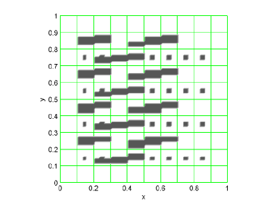
(a) Case I

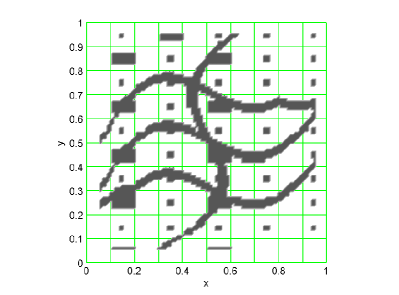
(b) Case II

Figure 3: Different permeability fields considered in the numerical experiments. Each permeability field has a different structures that model high conductivity channels within a homogeneous domain. The minimum (background) conductivity is taken to be $\kappa_{min}=1$, and the high-conductivity (gray regions) with value of $\kappa_{max}=10^{\eta}$ ($\eta$ = $4$ or $6$).

In this section, we present numerical examples to illustrate the applicability of the multiscale empirical interpolation method for solving nonlinear multiscale partial differential equations. Before presenting the individual examples, we review the computational domain used in constructing the GMsFEM basis functions. This computation is performed during the offline stage. We discretize with finite elements a nonlinear PDE posed on the computational domain $D=[0,1]\times[0,1]$. For constructing the coarse grid, we divide $[0,1]\times[0,1]$ into $10\times 10$ squares. Each square is divided further into $10\times 10$ squares each of which is divided into two triangles. Thus, the discretization parameters are $1/100$ for the fine-grid mesh and $1/10$ for the coarse-mesh. The fine-scale finite element vectors introduced in this section are defined on this fine grid. We recall that the fine-grid representation of a coarse-scale vector $z$ is given by $\Phi z$, which is a fine-grid vector.

Using the two grids, we construct the GMsFEM coarse space as described in Section 4. In the simulations, we consider two different permeability fields. These permeability fields, denoted by $\kappa$, contain channels of high conductivity and are shown in Figure 3. This figure shows fields with different structures that model high-conductivity channels within a homogeneous domain. The minimum conductivity value for this case is taken to be $\kappa_{min}=1$, and the high conductivity varies from channel to channel with a maximum value of $\kappa_{max}=10^{\eta}$ ($\eta$ = 4 or 6). Both permeability fields are represented by the fine mesh.

5.1 Nonlinear functions

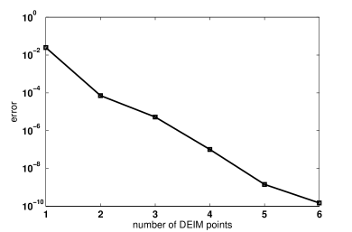
(a) $F_{1}$

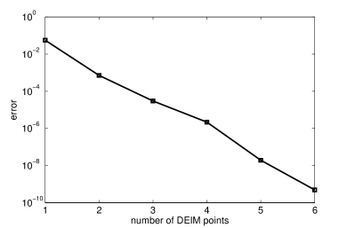
(b) $F_{2}$

Figure 4: Variations of the relative error between the approximate and the original nonlinear functions with the number of DEIM points.

To demonstrate the applicability of the multiscale empirical interpolation method in approximating nonlinear functions when using the multiscale framework, we consider two parametrized functions $F_{1}:\mathbb{R}^{n_{f}}\times[0,1]\mapsto\mathbb{R}^{n_{f}}$ and $F_{2}:\mathbb{R}^{n_{f}}\times[0,1]\mapsto\mathbb{R}^{n_{f}}$ given by

$$F_{1}(\Phi z;\mu) =\Big{(}\sin(2\pi\mu\Phi z)\cos(2\pi\mu\Phi z)\Big{)}^{2}e^{-2\pi\mu\Phi z}$$

$$F_{2}(\Phi z;\mu) =\frac{1}{1+\sin(2\pi\mu\Phi z)},$$ (35)

where $\mu\in[0,1]$. We follow the multiscale DEIM approach described in Section 3 to approximate the nonlinear function on the fine grid while evaluating at few selected points.

To check the capability of the multiscale DEIM to properly approximate the nonlinear function, we compute the relative error as the L₂-norm of the difference between the original and approximate functions: i.e.,

$$\|E\|_{2}=\frac{\|F-\widetilde{F}\|_{2}}{\|\widetilde{F}\|_{2}},$$ (36)

where $\widetilde{F}$ is obtained from the DEIM approximation. We consider $\Phi z$ as a multiscale solution of the elliptic problem obtained from a fine mesh of dimension 10201 (i.e., $N_{x}=N_{y}=n_{x}=n_{y}=$10) by solving $-\mbox{div}(\kappa\nabla u)=1$ in $D$ and $u=0$ on $\partial D$, where $\kappa$ is defined as in Case I with $\eta=4$ (see Figure 3). In Figure 4, we plot the relative error variations with the number of DEIM points. As expected, the error decreases as the number of DEIM points is increased. For instance, the relative error $\|E\|_{2}$ is equal to 7.18 10${}^{\mbox{-3}}$ and 7.14 10${}^{\mbox{-3}}$ when using only 2 DEIM points per region to approximate the nonlinear functions $F_{1}$ and $F_{2}$, respectively, defined on a fine mesh of dimension 10201. These results show the capability of the multiscale DEIM to reproduce the fine-scale representation of the nonlinear function while gaining in terms of computational cost through evaluating at only a few selected points.

In Figure 5, we compare the approximate functions obtained from DEIM using two points per region against the original function of dimension $n_{f}=10201$. The good agreement observed between the two sets of data shows the capability of DEIM to approximate the nonlinear function using a few selected points per region.

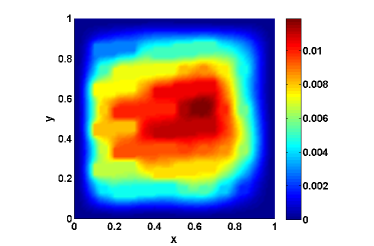
(a) $F_{1}$ - exact function

(b) $\widetilde{F}_{1}$ - approximate function

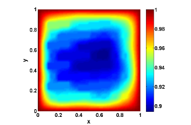
(c) $F_{2}$ - exact function

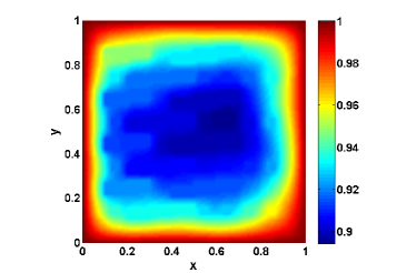
(d) $\widetilde{F}_{2}$ - approximate function

Figure 5: Comparison of the DEIM approximation with the original nonlinear function of dimension $n_{f}=10201$.

5.2 Nonlinear steady PDE

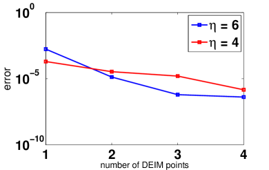
(a) Case I

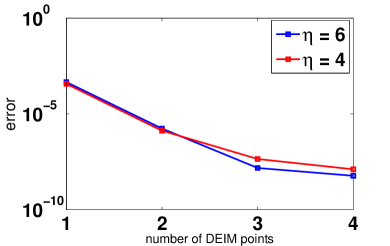
(b) Case II

Figure 6: Variations of the relative energy error between the multiscale and multiscale DEIM solutions with the number of DEIM points.

In this section, we consider a steady non-linear elliptic equation of the form

$$\mbox{div}\big{(}\kappa(x)\,\nabla u\big{)}=g(u,x,\mu)\,\,\,\,\text{in}\,\,\,\,D,$$ (37)

where

$$g(u,x,\mu)=(1+\sin(2\pi\mu u))e^{-2\pi\mu u}.$$ (38)

We consider permeability fields $\kappa$ that contain high-conductivity channels as shown in Figure 3. We use GMsFEM with Newton’s method to discretize and solve Equation (37) and employ the multiscale DEIM to approximate the nonlinear forcing term.

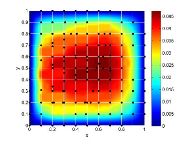
(a) Case I

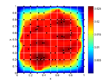
(b) Case II

Figure 7: Coarse grid and approximated solutions obtained from the multiscale DEIM approach using two DEIM points per region. Black dots denote the location of the DEIM points.

We define the relative energy error as

$$\|E\|_{\mbox{A}}=\sqrt{\frac{(\mbox{U}-\widetilde{\mbox{U}})^{T}{\mbox{A}}(\mbox{U}-\widetilde{\mbox{U}})}{\mbox{U}^{T}{\mbox{A}}\mbox{U}}},$$ (39)

where A is the fine-scale stiffness matrix that corresponds to (37). The errors are plotted in Figure 6 with respect to the number of DEIM points. Clearly, the use of a few DEIM points yields good approximation of the nonlinear forcing term and, consequently, the nonlinear PDE solution. Our numerical experiments show that the error does not depend on the contrast and it decreases as we increase the number of DEIM points. We refer to [21, 20, 15] for theoretical results on the error analysis of high-contrast problems.

For illustration purposes, in Figure 7, we show the approximate solutions obtained from the multiscale DEIM approach using two DEIM points per coarse region. The black dots denote the location of the DEIM points. These DEIM points show high absolute values of the modes representing the forcing terms in (37).

5.3 Nonlinear unsteady PDE

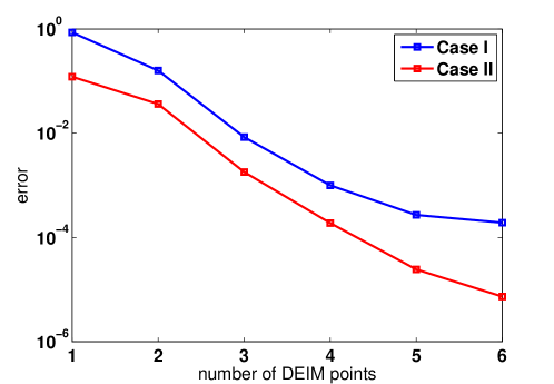
Figure 8: Variations of the relative energy error between the multiscale and multiscale DEIM solutions with the number of DEIM points.

As an example of a nonlinear unsteady problem, we consider the following time-dependent parabolic equation

$$\frac{\partial u}{\partial t}-\mbox{div}\big{(}\kappa(x;u,\mu)\,\nabla u\big{)}=h(x)\,\,\text{in}\,D,$$ (40)

where

$$\kappa(x;u,\mu)=\kappa_{q}(x)b_{q}(u,\mu),\;\;\;b_{q}(u,\mu)=e^{\mu u},\;\;\;h(x)=1+\sin(2\pi x_{1})\sin(2\pi x_{2}),$$

and the structure of the permeability fields $\kappa_{q}$ is shown in Figure 3. We employ the GMsFEM for space discretization and the Newton method to solve the nonlinear algebraic system at each time step as detailed in Section 4.3. Furthermore, we use multiscale DEIM, described in Section 3, to approximate the nonlinear functions and use multiscale POD (see Section 4.4) to identify the modes in the empirical interpolation. Without multiscale POD, the Newton method may converge slowly or may not converge when using $l_{2}$-inner-product-based POD [23]. In Figure 8, we plot the variation of the relative energy error between the multiscale and multiscale DEIM solutions with the number of DEIM points for the two configurations of the permeability field. The results are obtained for $\mu=10$. Multiscale DEIM approximates well the multiscale solutions as indicated by the small error values while significantly reducing the number of function evaluations.

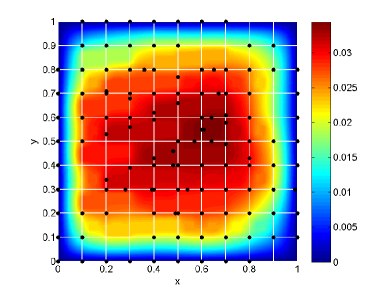
(a) Case I

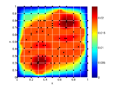
(b) Case II

Figure 9: Approximate solutions obtained from the multiscale DEIM approach using two DEIM points per region. Black dots denote the location of the DEIM points.

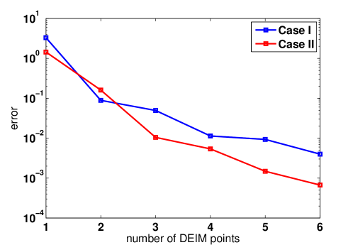
Figure 10: Variations of the relative energy error between the multiscale and multiscale DEIM solutions with the number of DEIM points.

In Figure 9, we show the approximate solutions obtained from the multiscale DEIM approach using two DEIM points per region. The black dots denote the location of the DEIM points.

We investigate the robustness of the multiscale DEIM approach with respect to moderate variations in the nonlinearity of the permeability field. As such, we run the forward problem while uniformly varying the value of the parameter $\mu$ of the nonlinear function $b_{q}$ over the interval $[5,10]$ with a step equal to one and store the snapshots of the nonlinear functions for each case. Then, we use all snapshots to compute the DEIM points and the index matrices of each region as described in Section 3. Next, we consider a nonlinear function $b_{q}(u,\mu)=e^{\mu u}$ with $\mu=8.5$ and show in Figure 10 the relative energy error variations with the number of DEIM points. Note that $\mu=8.5$ is not among the samples considered to compute the global DEIM points. Using a few DEIM points yields a good approximation. We mention that the simulation time of the final reduced order model is about $4\%$ of the computational time of running the fine-grid model. For instance, the relative energy error $\|E\|_{\mbox{A}}$ is equal to 4.96 10${}^{\mbox{-2}}$ and 1.05 10${}^{\mbox{-2}}$ when using only three DEIM points per region to approximate the nonlinear functions that appear in the residual $\widetilde{\mbox{R}}$ and the Jacobian $\widetilde{\mbox{J}}$ for the two configurations of the permeability field. Considering more DEIM points results in smaller error values. These results demonstrate the robustness of the model reduction approach based on combining the multiscale framework and DEIM. We have also tested this approach with different right-hand-sides and observed similar results.

6 Conclusions

In this paper, we propose a multiscale empirical interpolation for solving nonlinear multiscale partial differential equations. The proposed method uses the Generalized Multiscale Finite Element Method (GMsFEM) which constructs multiscale basis functions on a coarse grid to solve the nonlinear problem. To approximate inexpensively nonlinear functions that arise in the residual and Jacobians, we design multiscale empirical interpolation techniques that use empirical modes constructed based on local approximations of the nonlinear functions using weighted POD techniques. The proposed multiscale empirical interpolation techniques (1) divide the computation of the nonlinear function into coarse regions, (2) evaluate the contributions of the nonlinear functions in each coarse region taking advantage of a reduced-order solution representation, and (3) introduce multiscale Proper Orthogonal Decomposition techniques to find appropriate interpolation vectors. We demonstrate the applicability of the proposed methods on several examples of nonlinear multiscale PDEs that are solved with Newton methods. Our numerical results show that the proposed methods provide an accurate and robust framework for solving nonlinear multiscale PDEs on coarse grids while providing significant computational cost savings..

References

- [1] J.E. Aarnes. On the use of a mixed multiscale finite element method for greater flexibility and increased speed or improved accuracy in reservoir simulation. SIAM J. Multiscale Modeling and Simulation, 2:421–439, 2004.
- [2] J.E. Aarnes and Y. Efendiev. Mixed multiscale finite element for stochastic porous media flows. SIAM J. Sci. Comput., 30 (5):2319–2339, 2008.
- [3] T. Arbogast. Analysis of a two-scale, locally conservative subgrid upscaling for elliptic problems. SIAM J. Numer. Anal., 42(2):576–598 (electronic), 2004.
- [4] T. Arbogast and K.J. Boyd. Subgrid upscaling and mixed multiscale finite elements. SIAM J. Numer. Anal., 44(3):1150–1171 (electronic), 2006.
- [5] T. Arbogast, G. Pencheva, M.F. Wheeler, and I. Yotov. A multiscale mortar mixed finite element method. Multiscale Model. Simul., 6(1):319–346, 2007.
- [6] Maxime Barrault, Yvon Maday, Ngoc Cuong Nguyen, and Anthony T. Patera. An ‘empirical interpolation’ method: application to efficient reduced-basis discretization of partial differential equations. C. R. Math. Acad. Sci. Paris, 339(9):667–672, 2004.
- [7] S. Chaturantabut and D.C. Sorensen. Nonlinear model reduction via discrete empirical interpolation. SIAM J. Sci. Comput., 32(5):2737–2764, 2010.
- [8] C.-C. Chu, I. G. Graham, and T.-Y. Hou. A new multiscale finite element method for high-contrast elliptic interface problems. Math. Comp., 79(272):1915–1955, 2010.
- [9] Martin Drohmann, Bernard Haasdonk, and Mario Ohlberger. Reduced basis approximation for nonlinear parametrized evolution equations based on empirical operator interpolation. SIAM J. Sci. Comput., 34(2):A937–A969, 2012.
- [10] W. E and B. Engquist. Heterogeneous multiscale methods. Comm. Math. Sci., 1(1):87–132, 2003.
- [11] Y. Efendiev, J. Galvis, and T. Hou. Generalized multiscale finite element methods. Journal of Computational Physics, 251:116–135, 2013.
- [12] Y. Efendiev, J. Galvis, G. Li, and M. Presho. Generalized multiscale finite element methods. oversampling strategies. International Journal for Multiscale Computational Engineering, accepted, 2013.
- [13] Y. Efendiev, J. Galvis, M. Moon, R. Lazarov, and M. Sarkis. Generalized multiscale finite element method. symmetric interior penalty coupling. Journal of Computational Physics, accepted, 2013.
- [14] Y. Efendiev, J. Galvis, and F. Thomines. A systematic coarse-scale model reduction technique for parameter-dependent flows in highly heterogeneous media and its applications. Multiscale Model. Simul., 10:1317–1343, 2012.
- [15] Y. Efendiev, J. Galvis, and X.H. Wu. Multiscale finite element methods for high-contrast problems using local spectral basis functions. Journal of Computational Physics, 230:937–955, 2011.
- [16] Y. Efendiev and T. Hou. Multiscale Finite Element Methods: Theory and Applications, volume 4 of Surveys and Tutorials in the Applied Mathematical Sciences. Springer, New York, 2009.
- [17] Y. Efendiev, T. Hou, and V. Ginting. Multiscale finite element methods for nonlinear problems and their applications. Comm. Math. Sci., 2:553–589, 2004.
- [18] Y. Efendiev and A. Pankov. Numerical homogenization and correctors for nonlinear elliptic equations. SIAM J. Appl. Math., 65(1):43–68, 2004.
- [19] Y. Efendiev and A. Pankov. On homogenization of almost periodic nonlinear parabolic operators. Int. J. Evol. Equ., 1(3):203–209, 2005.
- [20] Juan Galvis and Yalchin Efendiev. Domain decomposition preconditioners for multiscale flows in high-contrast media. Multiscale Model. Simul., 8(4):1461–1483, 2010.
- [21] Juan Galvis and Yalchin Efendiev. Domain decomposition preconditioners for multiscale flows in high contrast media: reduced dimension coarse spaces. Multiscale Model. Simul., 8(5):1621–1644, 2010.
- [22] M. Ghommem, M. Presho, V. M. Calo, and Y. Efendiev. Mode decomposition methods for flows in high-contrast porous media. global?-local approach. Journal of Computational Physics, Vol. 253., pages 226?–238.
- [23] M. Hinze and S. Volkwein. Proper orthogonal decomposition surrogate models for nonlinear dynamical systems: error estimates and suboptimal control. In P. Benner, V. Mehrmann, and D.C. Sorensen, editors, Dimension Reduction of Large-Scale Systems, volume 45 of Lecture Notes in Computational Science and Engineering, pages 261–306. Springer Berlin Heidelberg, 2005.
- [24] T. Hughes, G. Feijoo, L. Mazzei, and J. Quincy. The variational multiscale method - a paradigm for computational mechanics. Comput. Methods Appl. Mech. Engrg., 166:3–24, 1998.
- [25] O. Iliev, R. Lazarov, and J. Willems. Variational multiscale finite element method for flows in highly porous media. Multiscale Model. Simul., 9(4):1350–1372, 2011.
- [26] P. Jenny, S.H. Lee, and H. Tchelepi. Multi-scale finite volume method for elliptic problems in subsurface flow simulation. J. Comput. Phys., 187:47–67, 2003.
- [27] M.F. Wheeler, G. Xue, and I. Yotov. A multiscale mortar multipoint flux mixed finite element method. ESAIM Math. Model. Numer. Anal., 46(4):759–796, 2012.