PROBING QUBIT BY QUBIT: PROPERTIES OF THE POVM AND THE INFORMATION/DISTURBANCE TRADEOFF

Abstract

We address the class of positive operator-valued measures (POVMs) for qubit systems that are obtained by coupling the signal qubit with a probe qubit and then performing a projective measurement on the sole probe system. These POVMs, which represent the simplest class of qubit POVMs, depends on $3+3+2=8$ free parameters describing the initial preparation of the probe qubit, the Cartan representative of the unitary coupling, and the projective measurement at the output, respectively. We analyze in some details the properties of the POVM matrix elements, and investigate their values for given ranges of the free parameters. We also analyze in details the tradeoff between information and disturbance for different ranges of the free parameters, showing, among other things, that i) typical values of the tradeoff are close to optimality and ii) even using a maximally mixed probe one may achieve optimal tradeoff.

1 Introduction

A common task in quantum technology is that of extracting information about the state of a physical system without destroying the information itself, i.e. possibly leaving part of it for another users. This is usually accomplished through indirect measurement, i.e. coupling the system of interest with a probe system and performing measurements on the probe [1]. The information on the system is thus provided by the probe and the system is not destroyed, though its state may be changed after the measurement. This measurement strategy may be described in terms of the sole system, neglecting the probe, by tracing out the probe degrees of freedom. This procedure returns a positive operator-valued measure (POVM) on the Hilbert space of the system, which describes both the statistics of the outcomes and the state reduction due to the measurement.[2, 3, 4, 5, 6] For qubit systems the simplest class of POVMs involves another qubit as probe and depends on $3+3+2=8$ free parameters, which describe the initial preparation of the probe qubit, the unitary operator coupling the two qubits, and the projective measurement at the output, respectively.

In this paper, we address the properties of this class of POVMs as a function of the free parameters. In particular, in order to obtain information about their typical values, the distribution of POVMs’ matrix elements is analyzed for random choices of the free parameters in different ranges. Besides, we analyze in some details the tradeoff between information and disturbance, showing that typical values of the tradeoff are close to optimality and that even using a maximally mixed probe one may still achieve optimal tradeoff.

The paper is structured as follow. In Section 2 we describe in details the measurement scheme and the range of variation of the free parameters. In doing this we review the Cartan decomposition of two-qubit unitaries and provide the characterization of the POVM elements, the so-called effects [7, 8, 9]. In Section 3 we analyze the distribution of the POVM matrix elements as a function of the free parameters. In Section 4 the quantification of information and disturbance is briefly reviewed and the corresponding distribution of fidelities is studied as a function of the free parameters. Section 5 closes the paper with some concluding remarks.

2 The measurement scheme

Let us consider the following scheme of measurement, which exploits a probe qubit in order to gain information on a signal qubit. In the first stage the probe qubit is prepared in a known state and then the signal and the probe are coupled by a unitary operator. Finally, a projective measurement is performed on the sole probe system (see Fig. 1).

Figure 1: (Color online) Schematic diagram of a general measurement scheme exploiting a probe qubit in order to gain information on a signal qubit prepared in an unknown state $\rho_{S}$. In the first step the probe qubit is prepared in a known state $\rho_{P}$, then the signal and the probe are coupled by the two-qubit unitary $U$ and, finally, a projective measurement described by the projection-valued measure $\{P,\mathbb{I}-P\}$ is performed on the sole probe qubit.

The unitary operator $U$ works on $\mathbb{C}^{2}\otimes\mathbb{C}^{2}$, and we assume its determinant to be equal to $1$, in order to have $U\in SU(4)$. We refer to the Hilbert space of the system as ${H}_{S}$, while the Hilbert space of the probe is ${H}_{P}$. The state of the probe $\rho_{P}\in\mathit{S}({H}_{P})$ in the Bloch representation may be written as

$$\rho_{P}=\frac{1}{2}(\mathbb{I}+\boldsymbol{r}\cdot\boldsymbol{\sigma})$$

where the Bloch vector $\boldsymbol{r}=(r_{1},r_{2},r_{3})$ is given by

$$r_{1}=\sqrt{2\mu-1}\sin\theta\cos\phi\,,\quad r_{2}=\sqrt{2\mu-1}\sin\theta\sin\phi\,,\quad r_{3}=\sqrt{2\mu-1}\cos\theta$$

where $\mu\in[1/2,1]$ is the purity of the probe system, and $\theta\in[0,\pi]$, $\phi\in[0,2\pi)$.

The projective measurement, performed on the probe system, is described by $P=\left|{\xi}\right\rangle\left\langle{\xi}\right|$, where $\left|{\xi}\right\rangle=\cos\frac{\alpha}{2}\left|{0}\right\rangle+e^{i\beta}\sin\frac{\alpha}{2}\left|{1}\right\rangle$ and $\alpha\in[0,\pi]$ and $\beta\in[0,2\pi)$. Since the probe is a qubit, then the projective measurement is composed by $P$ and $\mathbb{I}-P$.

The unitary operator $U\in SU(4)$ depends on $15$ parameters. In order to reduce this number, we use the Cartan decomposition, which allows us to replace $U$ with the operator $V$, working on both system and probe, depending on just 3 parameters, plus four local unitary operators, namely $R_{1},R_{2},S_{1},S_{2}\in SU(2)$:[9]

$$U=(R_{1}\otimes R_{2})V(S_{1}\otimes S_{2})$$

The operator $V$ is given by:

$$V=\mathrm{exp}\left\{-i\left[\frac{1}{2}(\alpha_{1}-\alpha_{2})\,\Sigma_{1}+\frac{1}{2}(\alpha_{1}+\alpha_{2})\,\Sigma_{2}+\alpha_{3}\,\Sigma_{3}\right]\right\}$$

where $\Sigma_{i}=1/2\ \sigma_{i}\otimes\sigma_{i}$ and the parameters $\alpha_{i}$ should satisfy the following constraints:

$$-\pi\leq\alpha_{1}\leq 0$$ (1a)

$$0\leq\alpha_{2}\leq-\alpha_{1}$$ (1b)

$$\alpha_{1}+\alpha_{2}\leq 2\alpha_{3}\leq 0$$ (1c)

Moreover, if $\alpha_{3}=0$, then $\alpha_{1}-\alpha_{2}\geq-\pi$. Clearly, the Cartan decomposition does not reduce the number of parameter of $U$, since each local operator depends on 3 parameters. However, as we will see, for our purposes, the local operators could be neglected.

The measurement scheme given above can be described by a POVM on the Hilbert space ${H}_{S}$. The operators which compose a POVM are often referred to as effects. An effect represents an apparatus with dicotomic outcome (yes$/$no). Therefore, each effect of a POVM is connected to a single outcome of the apparatus, and gives the probability that its outcome occurs.[10, 11]. The effects composing this POVM are given by the following equation (Naimark Theorem): [12]

$$\Pi=\mathrm{Tr}_{P}\left[{(\mathbb{I}\otimes\rho_{P})\ U^{\dagger}\ (\mathbb{I}\otimes P)\ U}\right]$$ (2)

Notice that, since the PVM on the probe system is $\{P,\mathbb{I}-P\}$, then the POVM on ${H}_{S}$ is composed by two effects, i.e. $\{\Pi,\mathbb{I}-\Pi\}$, and it is fully characterized by the matrix elements of $\Pi$. The Cartan decomposition of $U$ may be exploited to rewrite Eq. (2) as follows $\Pi=S_{1}^{\dagger}\ \mathrm{Tr}_{P}\left[{(\mathbb{I}\otimes S_{2}\,\rho_{P}\,S_{2}^{\dagger})\ V^{\dagger}\ (\mathbb{I}\otimes R_{2}^{\dagger}\,P\,R_{2})\,V}\right]S_{1}\,.$ The local operators $R_{2}$ and $S_{2}$ are rotations in the qubit space ${H}_{P}$ and may be easily eliminated by a suitable reparametrization of the probe state $\rho_{P}$ and the projector $P$. The rotation $S_{1}$ corresponds to an operation performed on the system qubit before the measurement, and it does not affect the properties of the POVM itself [13]. We thus assume, without loss of generality, to have $S_{1}=\mathbb{I}$. Overall, the effect $\Pi\in\mathit{B}({H}_{S})$ may be written as

$$\Pi=\mathrm{Tr}_{P}\left[{(\mathbb{I}\otimes\rho_{P})\ V^{\dagger}\ (\mathbb{I}\otimes P)\ V}\right]$$ (3)

In the Pauli basis we have $\Pi=a_{0}\ \mathbb{I}+\boldsymbol{a}\cdot\boldsymbol{\sigma}$, with $\boldsymbol{a}=(a_{1},a_{2},a_{3})$, where $a_{0}=\frac{1}{2}\mathrm{Tr}\left[{\Pi}\right]$ and $\boldsymbol{a}=\frac{1}{2}\mathrm{Tr}\left[{\Pi\,\boldsymbol{\sigma}}\right]$. These coefficients depend on the eight free parameters $\alpha_{1}$, $\alpha_{2}$, $\alpha_{3}$, $\mu$, $\theta$, $\phi$, $\alpha$ and $\beta$. The analytic expression of the coefficients of $\Pi$ is given in the A, and will be used in Section 3 to characterize the properties of the POVM as a function of the free parameters.

3 Characterization of $\Pi$

As mentioned above, the operator $\Pi$ fully describes the POVM and, in turn, the measurement scheme. $\Pi$ is an effect, i.e. a bound operator, which is positive, and hence selfadjoint, and with eigenvalues smaller that 1. Sometimes these conditions are synthetically expressed as $0\leq\Pi\leq\mathbb{I}$ which, after straightforward calculations, may be shown equivalent to the following constraints:

$$0\leq|a|\leq 1/2$$ (4a)

$$|a|\leq a_{0}\leq 1-|a|$$ (4b)

where $|a|=\sqrt{a_{1}^{2}+a_{2}^{2}+a_{3}^{2}}$ and $(a_{0},\boldsymbol{a})\in\mathbb{R}^{4}$. If $a_{0}=|a|=1/2$, then $\Pi$ is a projector, i.e. an extremal point of the set of effects.

We now study in some details the distribution of the parameters $a_{0}$ and $|a|$ within the physical region determined by Eq. (4). First of all, we check whether, taking at random the values of the free parameters in their whole ranges, we obtain a uniform distribution in the physically allowed region. This is indeed the case, as it can be seen by looking at the medium gray points in the three panels of Fig. 2.

Let us now analyze how the purity $\mu$ of the probe system affects the properties of the POVMs: in the left panel of Fig. 2 light gray points are obtained by selecting $\mu$ in the range $[0.5,0.7]$, while the black ones are obtained using a range $[0.5,0.51]$. As it is apparent from the plot, the coefficient $a_{0}$ is quite sensitive to the purity and its range is narrowing for decreasing purity. This behaviour can be understood by the analytic form of coefficient $a_{0}$, we have

$$a_{0}=\frac{1}{4}(2+\sqrt{2\mu-1}\ f(\alpha_{1},\alpha_{2},\alpha_{3},\theta,\phi,\alpha,\beta))$$

where $f(\alpha_{1},\alpha_{2},\alpha_{3},\theta,\phi,\alpha,\beta)\in[-2,2]$. When $\mu=1$, $a_{0}\in[0,1]$, while for $\mu=1/2$ the only allowed value is in fact $a_{0}=1/2$.

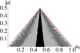
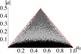
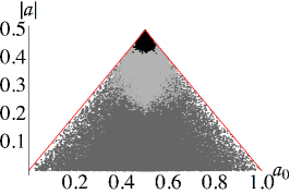
Figure 2: (Color online) The distributions of $\{a_{0},|a|\}$ inside the allowed region given by Eq. (4) (individuated by the red line) for different ranges of the free parameters. In all the plots the medium gray points correspond to the POVMs obtained with all the free parameters chosen at random in their whole ranges of variation. The light gray points and the black ones corresponds to POVMs obtained choosing the free parameters at random in restricted ranges. In the left panel, we show the POVMs corresponding to different ranges for $\mu$: light gray points are for $\mu\in[0.5,0.7]$, while the black ones corresponds to $\mu\in[0.5,0.51]$. The center panel describes both the situations in which the range of all the parameters $\alpha_{i}$ tends to 0 and in which the range of $\alpha_{1}$ tends to $-\pi$, the range of $\alpha_{2}$ tends to $\pi$ and the one of $\alpha_{3}$ tends to 0 (see text). The right panel shows the case in which the range of $\alpha_{1}$ tends to $-\pi$, the range of $\alpha_{2}$ tends to 0 and the one of $\alpha_{3}$ tends to $-\pi/2$.

The distribution of the coefficients of $\Pi$ also depends on the parameters $\alpha_{1}$, $\alpha_{2}$ and $\alpha_{3}$ of the unitary operation. Looking at the central panel of Fig. 2, medium gray points are again obtained for the free parameters randomly chosen in their whole range, whereas light gray points are given for $\alpha_{1}\in[-\pi/3,0]$ and black ones for $\alpha_{1}\in[-\pi/10,0]$. Notice that any constraint on $\alpha_{1}$ is also limiting the ranges of the other two parameters $\alpha_{2}$ and $\alpha_{3}$, through the conditions given in (1). As it is apparent from the plot by shrinking the range of the parameter $\alpha_{1}$ the range of $|a|$ is also shrinking. The limiting case is $\alpha_{1}\rightarrow 0$ (and thus $\alpha_{2},\alpha_{3}\rightarrow 0$), corresponding to $|a|\rightarrow 0$ and $a_{0}\in[0,1]$, i.e. to the trivial case $V=\mathbb{I}\otimes\mathbb{I}$ and $\Pi=\mathrm{Tr}_{P}\left[{\rho_{P}\ P}\right]\mathbb{I}_{S}$.

Consider now the case in which the range of $\alpha_{2}$ is narrowed up to the point $\pi$: the constraints given for the $\alpha_{i}$’s force the range of $\alpha_{1}$ to $-\pi$ and the range of $\alpha_{3}$ to 0. This case is again described by the central panel Fig. 2, but now the light gray points are obtained taking $\alpha_{1}\in[-\pi,-3/4\pi]$, $\alpha_{2}\in[3/4\pi,-\alpha_{1}]$ (notice that the ranges of $\alpha_{1}$ and $\alpha_{2}$ are chosen in order to always keep $\alpha_{3}\leq 0$). The black points now correspond to $\alpha_{1}\in[-\pi,-9/10\pi]$ and $\alpha_{2}\in[9/10\pi,-\alpha_{1}]$. It is worth noting that, when $\alpha_{1}=-\pi$, $\alpha_{2}=\pi$ and $\alpha_{3}=0$, then $V=i\,\sigma_{x}\otimes\sigma_{x}$ and $\Pi=i\,\mathrm{Tr}_{P}\left[{\rho_{P}\ \sigma_{x}P\sigma_{x}}\right]\mathbb{I}_{S}$.

Let us now consider the right panel Fig. 2. Here, we analyze the distribution of the coefficients $\{a_{0},|a|\}$ when the range of $\alpha_{3}$ is narrowed to the point $-\pi/2$. Due to the constraints, we have that also the ranges of $\alpha_{1}$ and $\alpha_{2}$ tend to a single point $\alpha_{1}=-\pi$ and $\alpha_{2}=0$. The light gray points correspond to $\alpha_{1}\in[-\pi,-3/4\pi]$, $\alpha_{2}\in[0,-\alpha_{1}/3]$ and $\alpha_{3}\in[(\alpha_{1}+\alpha_{2})/2,-\pi/6]$, whereas black points are for $\alpha_{1}\in[-\pi,-9/10\pi]$, $\alpha_{2}\in[0,-\alpha_{1}/9]$ and $\alpha_{3}\in[(\alpha_{1}+\alpha_{2})/2,-\pi/3]$. It is clear that the distribution of the coefficients tends to shrink to the region close to $a_{0}=1/2$ and $|a|=1/2$. We remark that an effect with $a_{0}=|a|=1/2$ is a projector. In fact, for $\alpha_{1}=-\pi$, $\alpha_{2}=0$ and $\alpha_{3}=-\pi/2$, the operator $V$ is the swap operator and $\Pi$ reduces to $\left|{\xi}\right\rangle\left\langle{\xi}\right|$.

Finally, we mention that the parameters $\theta$, $\phi$, $\alpha$ and $\beta$ modify the range of the coefficients $a_{i}$’s, but their changes do not influence neither $a_{0}$ nor $|a|$.

4 Tradeoff between information and disturbance

If we perform the measurement of an observable on a system prepared in a state which is not an eigenstate of the measured observable, the post-measurement state is different from the initial state of the system, i.e. the system has been disturbed. At the same time, the outcome of the measurement provides some amount of information about the state of the system under investigation before the measurement. A question thus arises on whether one may quantify the overall information that can be extract from a measurement as well as the disturbance introduced by the same measurement[1, 14, 15, 16, 17, 18, 19, 20].

Consider the case in which a system in a generic pure state $\left|{\psi}\right\rangle$ undergoes a measurement described by a POVM, composed by the effects $E_{k}$’s. The post-measurement state conditioned on the occurrence of the outcome $k$ is given by

$$\left|{\psi_{k}}\right\rangle=\frac{\sqrt{E_{k}}}{\sqrt{p_{k}}}\left|{\psi}\right\rangle$$

where $p_{k}$ is the probability distribution of the outcomes $k$’s for the state $\left|{\psi}\right\rangle$. Therefore, the disturbance introduced from the measurement is given by the fidelity of disturbance $F=\int\!d\psi\,\sum_{k}\,p_{k}\,|\langle{\psi_{k}}|{\psi}\rangle|^{2}$ where the integral is made on all the possible initial state (e.g. for qubit, giving a parametrization on the Bloch sphere, we have $d\psi=d\theta d\phi\sin\theta$). Notice that, if $F$ is equal to 1, then the measurement is not disturbing the system. When the outcome of the measurement is $k$, we may infer that the initial state was $\left|{\phi_{k}}\right\rangle$, where $\{|\phi_{h}\rangle\}$ is an arbitrary set of states. Therefore, measuring the observable, we obtain some information. The gained information is given by the fidelity of information $G=\int\!d\psi\,\sum_{k}\,p_{k}\,|\langle{\psi}|{\phi_{k}}\rangle|^{2}$. For the qubit POVM of Eq. (2) the above expressions reduce to

$$F =\frac{1}{6}\left(2+\left|\mathrm{Tr}\left[{\sqrt{\Pi}}\right]\,\right|^{2}+\left|\mathrm{Tr}\left[{\sqrt{\mathbb{I}-\Pi}}\right]\,\right|^{2}\right)$$

$$G =\frac{1}{6}\Bigg{(}2+\langle{\phi_{0}}|\Pi|\phi_{0}\rangle+\langle{\phi_{1}}|\mathbb{I}-\Pi|\phi_{1}\rangle\Bigg{)}$$

The ostensible freedom in the choice of the set of states $\left|{\phi_{k}}\right\rangle$’s is removed by maximizing the fidelity of information $G$. Then, each state $\left|{\phi_{k}}\right\rangle$ has to be the eigenstate of the effect $E_{k}$ with the maximum eigenvalue. Upon exploiting Eq. (2), one may show that $F$ and $G$ have to satisfy the following relation[1]

$$(F-\frac{2}{3})^{2}+4(G-\frac{1}{2})^{2}\leq\frac{1}{9}\,$$ (5)

which expresses quantitatively the tradeoff between information and disturbance in quantum measurement on a qubit. A POVM leading to fidelities $F$ and $G$ saturating the above inequality is said to be optimal.

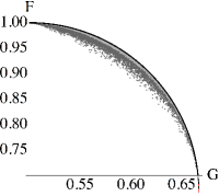
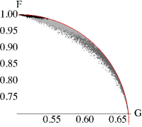
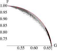
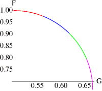
Figure 3: (Color online) Tradeoff between the information fidelity $G$ and the disturbance fidelity $F$ for different ranges of the free parameters. In the three panels on the left, the medium gray points correspond to POVM obtained by choosing the free parameters in their whole range, whereas the light gray points and the black ones to POVMs for restricted ranges of some parameters. The solid red line denotes the optimal tradeoff, i.e. the values saturating the inequality in Eq. (5). In the most left panel, we show the distribution of $G$ and $F$ for different ranges of the probe purity: light gray points correspond to $\mu\in[0.5,0.7]$ and the black ones to $\mu\in[0.5,0.51]$. The second plot shows results for different ranges of $\alpha_{1}$: the light gray points corresponds to $\alpha_{1}\in[-\pi/3,0]$ and the black ones for $\alpha_{1}\in[-\pi/10,0]$. The same distributions are obtained for $\alpha_{1}\in[-\pi,-3/4\pi]$, and $\alpha_{2}\in[3/4\pi,-\alpha_{1}]$ (light gray points), and $\alpha_{1}\in[-\pi,-9/10\pi]$ and $\alpha_{2}\in[9/10\pi,-\alpha_{1}]$ (black points). In the third panel the light gray points corresponds to $\alpha_{1}\in[-\pi,-3/4\pi]$, $\alpha_{2}\in[0,-\alpha_{1}/3]$ and $\alpha_{3}\in[(\alpha_{1}+\alpha_{2})/2,-\pi/6]$, whereas black points are for $\alpha_{1}\in[-\pi,-9/10\pi]$, $\alpha_{2}\in[0,-\alpha_{1}/9]$ and $\alpha_{3}\in[(\alpha_{1}+\alpha_{2})/2,-\pi/3]$. The last panel on the right shows the fidelities obtained using a $C_{not}$ gate to couple signal and probe, as a function of the population parameter $\theta$ of the probe.

In order to understand whether there is some typical value of the tradeoff we have performed a study of the distribution of the pairs $\{G,F\}$ for POVMs obtained for different distributions of the free parameters. In particular, we have considered the same ranges used in the previous Section for $\mu$ and the $\alpha_{k}$’s. The results are shown in Fig. 3, where again, the medium gray points are obtained by taking at random the free parameters into their whole range of variation.

In the left panel of Fig. 3, the distribution of $\{G,F\}$ is shown for different ranges of the purity $\mu$ of the probe system. In particular, light gray points are taken for $\mu\in[0.5,0.7]$, while the black ones are taken for $\mu\in[0.5,0.51]$. As it is apparent from the plot, by narrowing the range of $\mu$ the resulting POVMs become closer and closer to the optimal ones. In the limiting case of $\mu=\frac{1}{2}$ all the resulting POVMs have a tradeoff falling on the optimal curve of Eq. (5), i.e. all the POVMs are optimal. In order to have a more detailed picture, the histograms of their distribution are shown in Fig. 4: in the left panel, the POVMs are generated by choosing at random the parameters into their whole ranges. The histogram displays a distribution with a maximal value at the point $G=1/2$ and $F=1$, i.e. POVMs that neither gain information, nor disturb the state of the system. Moreover, it is apparent that not all the produced POVMs are optimal. The second histogram is obtained by taking at random $\mu$ between $0.5$ and $0.75$; in this case the distribution is different from zero for values of $F$ and $G$ near the optimal limit. In the right histogram, the distribution is taken for $\mu=1/2$: all the POVMs are optimal, but the distribution has a peak at the point $G=1/2$, $F=1$. Overall, the emerging picture is that even using a maximally mixed probe it is possible to saturate the optimal tradeoff. On the other hand, in this case the typical POVM is the non-informative one $\Pi=\mathbb{I}$. Still, it is possible to find POVMs with $G=F=2/3$, that is a measurement which extracts maximal information from the system and introduces a maximal disturbance. The two-qubit operator that gives this kind of POVMs is the swap operator $V(-\pi,0,-\pi/2)$.

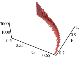
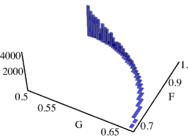
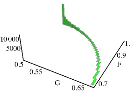
Figure 4: (Color online) The distribution of the POVMs as a function of $G$ and $F$. The first histogram is obtained by taking $\mu$ into its whole range. The second one for $\mu\in[0.5,0.75]$. The last one for $\mu=1/2$.

In the other panels of Fig. 3, we show how the distribution of the fidelities $\{G,F\}$ is affected by the ranges of $\alpha_{1}$, $\alpha_{2}$ and $\alpha_{3}$. In particular, the second panel refers to the case in which the range of the parameter $\alpha_{1}$ is progressively shrinking to the single point $\alpha_{1}=0$. As previously said, the constraints on the parameters $\alpha_{i}$’s force the other two parameters $\alpha_{2}$ and $\alpha_{3}$ to narrow their ranges into the single point $\alpha_{2}=\alpha_{3}=0$. The light gray points are taken for $\alpha_{1}\in[-\pi/3,0]$ and black ones for $\alpha_{1}\in[-\pi/10,0]$. The behavior of the distribution is quite clear: it collapses into the point $G=1/2$ and $F=1$, when $\alpha_{i}$’s $\rightarrow 0$. We recall that the corresponding POVMs are proportional to the identity $\mathbb{I}_{S}$.

The second panel of Fig. 3 also describes the trend of the distribution when the range of $\alpha_{2}$ is narrowed to the point $\pi$. Again, the constraints force the range of $\alpha_{1}$ to $-\pi$ and the range of $\alpha_{3}$ to 0. In this case, the light gray points are obtained taking $\alpha_{1}\in[-\pi,-3/4\pi]$, $\alpha_{2}\in[3/4\pi,-\alpha_{1}]$, while the black ones are taken for $\alpha_{1}\in[-\pi,-9/10\pi]$ and $\alpha_{2}\in[9/10\pi,-\alpha_{1}]$.

The third panel of Fig. 3 refers to the case in which the range of $\alpha_{3}$ is gradually reduced to the point $-\pi/2$, and therefore $\alpha_{1}\rightarrow-\pi$ and $\alpha_{2}\rightarrow 0$. The light gray points are taken for $\alpha_{1}\in[-\pi,-3/4\pi]$, $\alpha_{2}\in[0,-\alpha_{1}/3]$ and $\alpha_{3}\in[(\alpha_{1}+\alpha_{2})/2,-\pi/6]$, while black points stay for $\alpha_{1}\in[-\pi,-9/10\pi]$, $\alpha_{2}\in[0,-\alpha_{1}/9]$ and $\alpha_{3}\in[(\alpha_{1}+\alpha_{2})/2,-\pi/3]$. The distribution of $\{G,F\}$ collapses into the point $F=G=2/3$. In fact, for $\alpha_{1}=-\pi$, $\alpha_{2}=0$ and $\alpha_{3}=-\pi/2$, we obtain a projective measurement, giving as more information as possible about the system, at the price of introducing a considerable disturbance.

Finally, in the right panel of Fig. 3, we show the fidelities obtained by using a $C_{not}$ gate to couple the system and the probe qubit and then measuring $\sigma_{3}$ on the probe. In particular, we have considered the fidelities obtained by varying the $\theta$ parameter of the probe: the red portion of the curve corresponds to $\theta\in[0,\pi/8]$, the blue one to $\theta\in[\pi/8,\pi/4]$, green is for $\theta\in[\pi/4,3/8\pi]$, and magenta for $\theta\in[3/8\pi,\pi/2]$. As it is apparent from the plot, we confirm the known optimality[14, 15] of the resulting POVMs. Notice that, since the Cartan decomposition has been used to obtain the coefficients of the effect $\Pi$, we need to find the operator $V(\alpha_{1},\alpha_{2},\alpha_{3})$ connected to the $C_{not}$ gate. After straightforward calculation we find that $C_{not}=(R_{1}\otimes R_{2})\ V(-\frac{\pi}{2},\frac{\pi}{2},0)\ (S_{1}\otimes S_{2})$ where, as shown before, the local operators do not modify neither $F$ nor $G$.

5 Conclusions

In this paper, we have addressed the properties of the class of two-value qubit POVMs $\{\Pi,\mathbb{I}-\Pi\}$ that are obtained by coupling the signal qubit with a probe qubit and then performing a projective measurement on the sole probe system. These POVMs represent the simplest class of qubit POVMs and depends on $3+3+2=8$ free parameters describing the initial preparation of the probe qubit, the Cartan representative of the unitary coupling, and the projective measurement at the output, respectively. We have obtained the analytic expression of the coefficients $(a_{0},a_{1},a_{2},a_{3})$ of the effect $\Pi$ in the Pauli basis and have used these expressions to understand which parameters are relevant to specific properties of the POVMs. In particular, for the distribution of $\{a_{0},|a|\}$ we found that the relevant parameters are the purity $\mu$ of the probe system and the parameters defining the Cartan representative of the unitary coupling. We have also analyzed in details the tradeoff between information and disturbance for different ranges of the free parameters, showing, among other things, that i) typical values of the tradeoff are close to optimality and ii) even using a maximally mixed probe one may achieve optimal tradeoff (using a swap gate to couple the signal and the probe qubit), though the typical POVM is the non-informative one $\Pi=\mathbb{I}$.

Appendix A The matrix elements the effect $\Pi$ in the Pauli basis

The effect $\Pi=a_{0}\ \mathbb{I}+\boldsymbol{a}\cdot\boldsymbol{\sigma}$ has the following coefficient:

$$a_{0}= \frac{1}{4}(2+\sqrt{2\mu-1}\,(\cos\alpha\cos\theta\,(\cos\alpha_{1}+\cos\alpha_{2})+2\cos\alpha_{3}\sin\alpha\sin\theta$$

$$(\cos(\frac{\alpha_{1}+\alpha_{2}}{2})\cos\beta\cos\phi+\cos(\frac{\alpha_{1}-\alpha_{2}}{2})\sin\beta\sin\phi)))$$

$$a_{1}= \frac{1}{4}(2\cos\beta\sin\alpha\sin(\frac{\alpha_{1}+\alpha_{2}}{2})\sin\alpha_{3}$$

$$+\sqrt{2\mu-1}\,(\cos\alpha\,(\sin\alpha_{1}-\sin\alpha_{2})\sin\theta\sin\phi-2\cos\alpha_{3}\cos\theta\sin\alpha\sin(\frac{\alpha_{1}-\alpha_{2}}{2})\sin\beta))$$

$$a_{2}= \frac{1}{4}(2\sin\alpha\sin(\frac{\alpha_{1}-\alpha_{2}}{2})\sin\alpha_{3}\sin\beta$$

$$+\sqrt{2\mu-1}\,(2\cos\alpha_{3}\cos\beta\cos\theta\sin\alpha\sin(\frac{\alpha_{1}+\alpha_{2}}{2})-\cos\alpha\cos\phi\,(\sin\alpha_{1}+\sin\alpha_{2})\sin\theta))$$

$$a_{3}= \frac{1}{4}(\cos\alpha\,(\cos\alpha_{2}-\cos\alpha_{1})$$

$$+2\sqrt{2\mu-1}\sin\alpha\sin\alpha_{3}\sin\theta\,(\cos(\frac{\alpha_{1}-\alpha_{2}}{2})\cos\phi\sin\beta-\cos(\frac{\alpha_{1}+\alpha_{2}}{2})\cos\beta\sin\phi))$$

References

- [1] K. Banaszek, Phys. Rev. Lett. 86 (2001) 1366
- [2] C. W. Helstrom, Int. J. Theor. Phys. 8 (1973) 361
- [3] C. W. Helstrom, Quantum Detection and Estimation Theory (Academic Press, New York, 1976)
- [4] A. S. Holevo, Statistical Structure of Quantum Theory, Lect.Not. Phys 61, (Springer, Berlin, 2001)
- [5] J. Bergou, J. Mod. Opt. 57 (2010) 160
- [6] M. G. A. Paris, Eur. Phys. J. ST 203 (2012) 61
- [7] B. Kraus and J. I. Cirac, Phys. Rev. A 63 (2001) 062309
- [8] J. Zhang, J. Vala, S. Sastry and K. B. Whaley, Phys. Rev. A 67 (2003) 042313
- [9] R. R. Tucci, ArXiv quant-ph/0507171
- [10] G. Ludwig, Foundation of Quantum Mechanics I (Springer-Verlag, New York, 1983)
- [11] K. Kraus, States, Effects, and Oprations (Springer-Verlag, Berlin, 1983)
- [12] M. A. Naimark, Iza. Akad. Nauk USSR, Ser. Mat. 4 (1940) 277; C.R. Acad. Sci. URSS 41 (1943) 359
- [13] C. Sparaciari, M. G. A. Paris, Phys. Rev. A 87 (2013) 012106
- [14] M. G. Genoni, M. G. A. Paris, Phys. Rev. A 71 (2005) 052307.
- [15] L. Mita, R. Filip, Phys. Rev. A 72 (2005) 034307
- [16] J. Fiurek, Phys. Rev. A 70 (2004) 032308
- [17] M. G. Genoni, M. G. A. Paris, Phys. Rev. A 74 (2006) 012301
- [18] M. G. Genoni, M. G. A. Paris, J. Phys. CP 67 (2007) 012029
- [19] S. Olivares, M. G. A. Paris, J. Phys. A 40 (2007) 7945
- [20] K. Banaszek, Open Syst. Inf. Dyn. 13, 1 (2006).