Chemical and kinematical properties of Galactic bulge stars surrounding the stellar system Terzan 5

Abstract

As part of a study aimed at determining the kinematical and chemical properties of Terzan 5, we present the first characterization of the bulge stars surrounding this puzzling stellar system. We observed 615 targets located well beyond the tidal radius of Terzan 5 and we found that their radial velocity distribution is well described by a Gaussian function peaked at $<v_{{\rm rad}}>=+21.0\pm 4.6$ km s^-1 and with dispersion $\sigma_{v}=113.0\pm 2.7$ km s^-1. This is the one of the few high-precision spectroscopic survey of radial velocities for a large sample of bulge stars in such a low and positive latitude environment (b=+1.7°). We found no evidence for the peak at $<v_{{\rm rad}}>\sim+200$ km s^-1 found in Nidever et al. (2012). The strong contamination of many observed spectra by TiO bands prevented us from deriving the iron abundance for the entire spectroscopic sample, introducing a selection bias. The metallicity distribution was finally derived for a sub-sample of 112 stars in a magnitude range where the effect of the selection bias is negligible. The distribution is quite broad and roughly peaked at solar metallicity ([Fe/H]$\simeq+0.05$ dex) with a similar number of stars in the super-solar and in the sub-solar ranges. The population number ratios in different metallicity ranges agree well with those observed in other low-latitude bulge fields suggesting ($i$) the possible presence of a plateau for $|$b$|<4$°  for the ratio between stars in the super-solar ($0<$[Fe/H]$<0.5$ dex) and sub-solar ($-0.5<$[Fe/H]$<0$ dex) metallicity ranges; ($ii$) a severe drop of the metal-poor component ([Fe/H]$<-0.5$) as a function of Galactic latitude.

1 INTRODUCTION

Terzan 5 is a stellar system located in the bulge of our Galaxy, at a distance of 5.9 kpc (Valenti et al. 2007, 2010). Because of the large and spatially varying extinction (Massari et al. 2012) critically affecting any optical observation of the system, its true nature remained hidden until near infrared (NIR) observations revealed its peculiar properties. In fact, by using J and K band data acquired with the Multi-conjugate Adaptive optics Demonstrator (MAD) mounted at the Very Large Telescope, Ferraro et al. (2009) discovered the presence of two distinct stellar populations. The analysis of high-resolution IR spectra (Origlia et al. 1997) obtained with NIRSPEC at the Keck II telescope, demonstrated that the two populations have different metallicities, the metal-poor component being sub-solar with [Fe/H]$=-0.25$ dex and the metal-rich one having [Fe/H]$=+0.27$ dex (Ferraro et al. 2009; Origlia et al. 2011). Recently, we discovered even a third, more metal-poor population with [Fe/H]$\simeq-0.8$ dex (Origlia et al. 2013; Davide Massari et al. in preparation). The analysis of the $\alpha$-elements also revealed that the two metal-poor populations are $\alpha$-enhanced, and therefore formed from gas mainly enriched by type II supernovae (SNII). Instead the metal-rich component has a solar [$\alpha$/Fe] ratio and thus we infer that it formed from gas further polluted by type Ia supernovae (SNIa). This abundance pattern, with the $\alpha$-elements being enhanced up to solar metallicity and then progressively decreasing towards solar values (see Origlia et al., 2011), is strikingly similar to what is typically observed for the bulge field stars (see for instance McWilliam & Rich 1994; Fulbright et al. 2007; Hill et al. 2011; Rich et al. 2012; Johnson et al. 2013; Ness et al. 2013). However it must be noticed that the precise metallicity at which the knee in the [$\alpha$/Fe] vs [Fe/H] trend occurs is still controversial, since measurements are quite scattered, and different elements as well as different studies provide somewhat different answers.

In order to investigate the kinematical and chemical properties of Terzan 5, we have collected spectra for more than 1600 stars in its direction. In this paper we focus on the properties of the bulge field population surrounding the system, with the aim of providing crucial information for future studies of both Terzan 5 and the bulge itself. In fact, this is a statistically significant sample of field stars which can be used for the purpose of decontaminating Terzan 5 population from non-members. Moreover, it is one of the few large samples of bulge stars spectroscopically investigated at low and positive latitudes (b$=+1.7$°), thus allowing interesting comparisons with other well studied bulge regions.

The paper is organized as follows. In Section 2 we present the spectroscopic sample analyzed in this work. In Section 3 we describe the analysis and the results concerning the radial velocities. In Section 4 we describe the chemical analysis and the metallicity distribution of the sub-sample of stars for which we determined iron abundances, and in Section 5 we summarize the results obtained.

2 THE SAMPLE

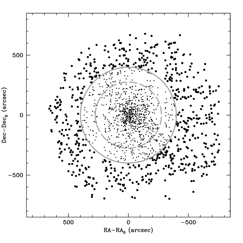
Figure 1: Spatial distribution of all the targets in our spectroscopic survey in the direction of Terzan 5. The center of gravity and tidal radius ($r_{t}\simeq 300\arcsec$) of Terzan 5 (from Lanzoni et al. 2010) are marked with a gray cross and a gray dashed circle, respectively. The targets discussed in the paper (shown as filled black circles) are all located at more than 400″ from the center (gray solid circle), well beyond the Terzan 5 tidal radius.

This study is based on a sample of 1608 stars within a radius of 800″from the center of Terzan 5 ($\alpha_{{\rm J}2000}=17^{\rm h}:48^{\rm m}:4^{\rm s\!.}85$, $\delta_{{\rm J}2000}=-24^{\circ}:46\arcmin:44\farcs 6$; see Ferraro et al. 2009; Lanzoni et al. 2010). While the overall survey will be described in a forthcoming paper (Francesco Ferraro et al. in preparation), in this work we focus on a sub-sample of stars representative of the field population surrounding Terzan 5. Given the value of the tidal radius of the system (r${}_{t}\simeq 300\arcsec$; Lanzoni et al. 2010; Miocchi et al. 2013), we conservatively selected as genuine field population members all the targets more distant than $400\arcsec$ from the center of Terzan 5. This sub-sample is composed of $615$ stars belonging to two different datasets obtained with FLAMES (Pasquini et al., 2002) at the ESO Very Large Telescope (VLT) and with DEIMOS (Faber et al. 2003) at the Keck II Telescope. Each target has been selected from the ESO-WFI optical catalog described in Lanzoni et al. (2010), along the brightest portion of the red giant branch (RGB), with magnitudes brighter than $I<18.5$. In order to avoid contamination from other sources, in the selection process of the spectroscopic targets we avoided stars with bright neighbors (I${}_{neighbor}<{\rm I_{star}}+1.0$) within a distance of 2″. The spatial distribution of the entire sample is shown in Figure 1, where the selected field members are shown as large filled circles.

The FLAMES dataset was collected under three different programs: 087.D-0716(B), PI: Ferraro; 087.D-0748(A), PI: Lovisi; and 283.D-5027(A), PI: Ferraro. All the spectra were acquired in the GIRAFFE/MEDUSA mode, allowing the allocation of 132 fibers across a $25\arcmin$ diameter field of view (FoV) in a single pointing. We used the GIRAFFE setup HR21, with a resolving power of 16200 and a spectral coverage ranging from 8484 Å to 9001 Å. This grating was chosen because it includes the prominent Ca II triplet lines, which are excellent features to measure radial velocities also in relatively low signal-to-noise ratio (SNR) spectra. Other metal lines (mainly Fe I) lie in this spectral range, thus allowing a direct measurement of the iron abundance. Multiple exposures (with integration times ranging from 1500 to 3000 s, according to the magnitude of the targets) were secured for the majority of the stars, in order to reach SNR$\sim$30 even for the faintest ($I\sim 18.5$) targets. The data reduction was performed with the FLAMES-GIRAFFE pipeline, including bias-subtraction, flat-field correction, wavelength calibration with a standard Th-Ar lamp, re-sampling at a constant pixel-size and extraction of one-dimensional spectra. Since a correct sky subtraction is particularly crucial in this spectral range (because of the large number of O₂ and OH emission lines), 15-20 fibers were used to measure the sky in each exposure. Then a master sky spectrum was obtained from the median of these spectra and it was subtracted from the target spectra. Finally, all the spectra were shifted to zero-velocity and in the case of multiple exposures they were co-added.

The DEIMOS dataset was acquired using the 1200 line/mm grating coupled with the GG495 and GG550 order-blocking filters, covering the $\sim$6500-9500 Å spectral range at a resolution of R$\sim$7000 at $\sim$8500 Å. The DEIMOS FoV is $16$′$\times 5$′, allowing the allocation of more than 100 slits in a single mask. The observations were performed with an exposure time of 600 s, securing SNR$\sim$50-60 spectra for the brightest targets and achieving SNR$\sim$15-20 for the faintest ones (I$\sim 17$). The spectra have been reduced by means of the package developed for an optimal reduction and extraction of DEIMOS spectra and described in Ibata et al. (2011).

3 RADIAL VELOCITIES

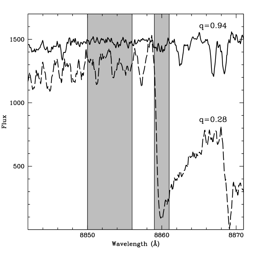
Figure 2: Examples of spectra poorly (solid line) and severely (dashed line) affected by the TiO molecular bands ($\lambda>8860$ Å). The gray regions highlight the wavelength ranges adopted to compute the $q$-parameter defined in the text (Section 4). For these two spectra very different values of $q$ have been obtained: $q=0.94$ and $q=0.28$ for the solid and dashed spectrum, respectively. According to the adopted selection criterion (q$>0.6$), the iron abundance has not been computed from the latter.

Radial velocities ($v_{\rm rad}$) for the target stars were measured by cross-correlating the observed spectra with a template of known velocity, following the procedure described in Tonry & Davis (1979) and implemented in the FXCOR software under IRAF. As templates we adopted synthetic spectra computed with the SYNTHE code (Sbordone et al., 2004). For most of the stars the cross-correlation procedure is performed in the spectral region $\sim$8490-8700 Å, including the prominent Ca II triplet lines that can be well detected also in noisy spectra. For some very cool stars, strong TiO molecular bands dominate this spectral region, preventing any reliable measurement of the Ca features (Figure 2 shows the comparison between two FLAMES spectra, with and without strong molecular bands). In these cases, the radial velocity was measured from the TiO lines by considering only the spectral region around the TiO bandhead at $\sim$8860 Å and by using as template a synthetic spectrum including all these features. Because several stars show both the Ca II triplet lines and weak TiO bandheads, for some of them the radial velocity has been measured independently using the two spectral regions. We always found an excellent agreement between the two measurements, thus ruling out possible offsets between the two $v_{\rm rad}$ diagnostics.

For the FLAMES dataset, where multiple exposures were secured for most of the stars, radial velocities were obtained from each exposure independently. The final radial velocity is computed as the weighted mean of the individual velocities (each corrected for its own heliocentric velocity), by using the formal errors provided by FXCOR as weights. For the DEIMOS spectra, we checked for possible velocity offsets due to the mis-centering of the target within the slit (see the discussion about this effect in Simon & Geha, 2007), through the cross-correlation of the A telluric band (7600-7630 Å). We found these offsets to be of the order of few km s^-1. The uncertainty on the determination of this correction (always smaller than 1 km s^-1) has been added in quadrature to that provided by FXCOR. The typical final error on our measured v_rad is $\sim 1.0$ km s^-1.

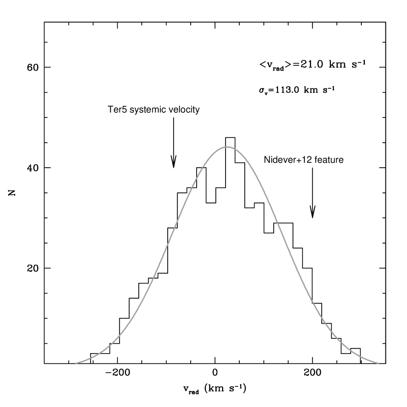
Figure 3: Radial velocity distribution for the 615 spectroscopic targets at $r>400\arcsec$. The mean value and dispersion are indicated. The bin size (20 km s^-1) is the same as that adopted by Nidever et al. (2012), but in our case no high velocity sub-components are found. The systemic velocity of Terzan 5 (v${}_{{\rm rad}}\simeq-83$ km s^-1) and the location of the subcomponent found in Nidever et al. (2012) (v${}_{{\rm rad}}\simeq 200$ km s^-1) are also marked with the black arrows for sake of comparison.

The distribution of the measured $v_{\rm rad}$ for the 615 targets is shown in Figure 3. It ranges from $-264.0$ km s^-1 to $+303.9$ km s^-1. By using a Maximum-Likelihood procedure, we find that the Gaussian function that best describes the distribution has mean $\langle v_{\rm rad}\rangle=21.0\pm 4.6$ km s^-1 and $\sigma_{v}=113.0\pm 2.7$ km s^-1. We converted radial velocities to Galactocentric velocities ($v_{\rm GC}$) by correcting for the Solar reflex motion (220 km s^-1; Kerr & Lynden-Bell 1986) and assuming as peculiar velocity of the Sun in the direction (l,b)$=$(53°,25°) $v=18.0$ km s^-1 (Schönrich et al., 2010). The conversion equation is then:

$$v_{{\rm GC}}=v_{{\rm rad}}+220[\sin(l)\cos(b)]+18[\sin(b)\sin(25)+\cos(l)\cos(25)\cos(l-53)],$$ (1)

where velocities are in km s^-1, and (l,b)=(3.8°, 1.7°) is the location of Terzan 5. The Galactocentric velocity distribution estimated in this way peaks at $<v_{{\rm GC}}>=47.7\pm 4.6$ km s^-1.

This value turns out to be in good agreement with the values found in the context of three recent kinematic surveys of the Galactic bulge: the BRAVA survey (Rich et al. 2007), the ARGOS survey (Freeman et al. 2013) and the GIBS survey (Zoccali et al. 2014). In fact, in fields located close to the Galactic Plane and with Galactic longitude as similar as possible to ours, Howard et al. (2008, see also Kunder et al. 2012) found $<v_{{\rm GC}}>=53.0\pm 10.3$ km s^-1 at (l,b)=(4°,-3.5°) for BRAVA, Ness et al. (2013) found $<v_{{\rm GC}}>=44.4\pm 3.8$ km s^-1 at (l,b)=(5°,-5°) for ARGOS and Zoccali et al. (2014) obtained $<v_{{\rm GC}}>=55.9\pm 3.9$ km s^-1 at (l,b)=(3°,-2°) for GIBS. Thus, all the measurements agree within the errors with our result. As for the velocity dispersion, our estimate ($\sigma_{v}=113\pm 2.7$ km s^-1) agrees well with the result of Kunder et al. (2012), who found $\sigma_{v}=106$ km s^-1, and with that of Zoccali et al. (2008) who measured $\sigma_{v}=112.5\pm 6.4$ km s^-1. Instead, it is larger than that quoted in Ness et al. (2013) $\sigma_{v}=92.2\pm 2.7$ km s^-1. Since their field is the farthest from ours among those selected for the comparison, we ascribe such a difference to the different location in the bulge. As a further check, we used the Besançon Galactic model (Robin et al. 2003) to simulate a field with the same size of our photometric sample (i.e., the WFI FoV) around the location of Terzan 5, and we selected all the bulge stars lying within the same color and magnitude limits of our sample. The velocity dispersion for these simulated stars is $\sigma_{v}=119$ km s^-1, in agreement with our estimate.

It is worth mentioning that Nidever et al. (2012) identified a high velocity ($v_{{\rm rad}}\sim$200 km s^-1) sub-component that accounts for about 10% of their entire sample of $\sim 4700$ bulge stars. Such a feature has been found in eight fields located at -4.3°$<$b$<2$°and 4°$<$l$<14$°. Nidever et al. (2012) suggest that such a high-velocity feature may correspond to stars in the Galactic bar which have been missed by other surveys because of the low latitude of the sampled fields. However, as is evident in Figure 3 (where we adopted the same bin-size used in Fig. 2 of Nidever et al. (2012) for sake of comparison), we do not find neither high-velocity peak nor isolated substructures in our sample, despite its low latitude. In fact, the skewness calculated for our distribution is $-0.02$, clearly demonstrating its symmetry. Also Zoccali et al. (2014) did not find any significant peak at such large velocity in the recent GIBS survey.

4 METALLICITIES

For a sub-sample of $284$ stars we were able to also derive metallicity. As already pointed out in Section 3, spectra of cool giants are affected by the presence of prominent TiO molecular bands. These bands make particularly uncertain the determination of the continuum level. While this effect has no consequences on the determination of radial velocities, it could critically affects the metallicity estimate. Therefore we limited the metallicity analysis only to stars whose spectra suffer from little contamination from the TiO bands. In order to properly evaluate the impact of the TiO bands in the considered wavelength range, we performed a detailed analysis of a large set of synthetic spectra and we defined a parameter $q$ as the ratio between the flux of the deepest feature of the TiO bandhead at 8860 Å (computed as the minimum value in the spectral range 8859.5 Å$<\lambda<$8861 Å) and the continuum level measured with an iterative 3 $\sigma$-clipping procedure in the adjacent spectral range, 8850Å$<\lambda<$8856 Å (see the shaded regions of Figure 2).

We found that the continuum level of synthetic spectra for stars with $q>0.8$ is slightly ($<2\%$) affected by TiO bands over the entire spectral range, while for stars with $0.6<q<0.8$ the region marginally ($<5\%$) affected by the contamination is confined between 8680 Å and 8850 Å. Instead, stars with $q<0.6$ have no useful spectral ranges (where at least one of the Fe I in our linelist falls) with TiO contamination weak enough to allow a reliable chemical analysis. We therefore analyzed targets with $q>0.8$ (counting 126 objects) using the full linelist (see Section 4.2), while for targets with $0.6<q<0.8$ (158 objects) only a sub-set of atomic lines lying in the safe spectral range $8680-8850$ Å has been adopted. All targets with $q<0.6$ (329 stars) have been excluded from the metallicity analysis. Hence the metallicity analysis is limited to 284 stars (corresponding to $\sim 46\%$ of the entire sample observed in the spectroscopic survey). In Section 4.5 we discuss the impact of this selection on the results of the paper.

4.1 Atmospheric parameters

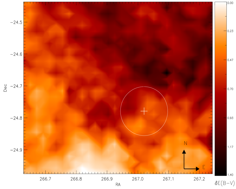
Figure 4: Reddening map in the direction of Terzan 5 covering the entire $\sim 25$′$\times 25$′ FoV. Dark colors correspond to regions of large extinction (see the color bar on the right). The center and tidal radius of Terzan 5 are marked for sake of comparison.

We derived effective temperatures (T_eff) and gravities ($\log$ $g$) photometrically. In order to minimize the effect of differential reddening we used the 2MASS catalog, correcting the (K, J-K) CMD for differential extinction according to our new wide-field reddening map, shown in Figure 4. This was obtained by applying to the optical WFI catalog the same procedure described in Massari et al. (2012). Because of the large incompleteness at the Main Sequence (MS) level we were forced to use red clump stars as reference. Since these stars are significantly less numerous than MS stars, the spatial resolution of the computed reddening map ($60\arcsec\times 60\arcsec$) is coarser than that ($8\arcsec\times 8\arcsec$) published in Massari et al. (2012) for the HST ACS field of view. However, despite this difference in resolution, the WFI reddening map agrees quite well with that for ACS in the overlapping region. Indeed for the stars in common between the two catalogs, the average difference between the differential reddening estimates is $\langle\Delta E(B-V)\rangle=0.01$ mag with a dispersion $\sigma=0.1$ mag. This latter value is also the uncertainty that we conservatively adopt for our color excess estimates.

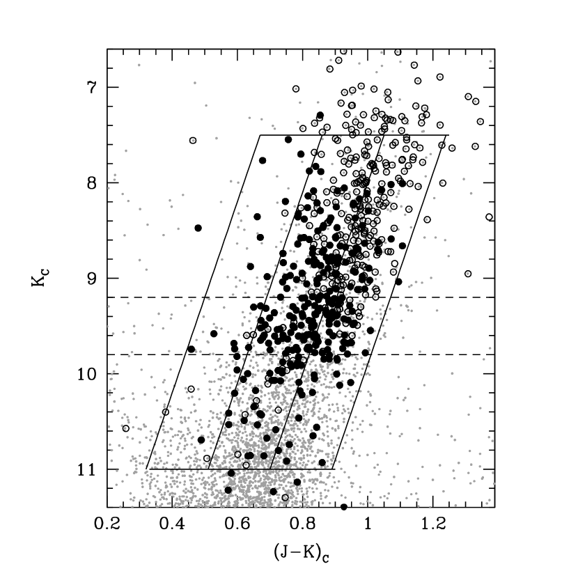
Figure 5: (K, J-K) CMD corrected for internal differential extinction, for all the stars located at $400\arcsec<r<800\arcsec$ from the center of Terzan 5, in our ESO-WFI photometric sample (small dots). The spectroscopic targets are shown with large symbols. The targets for which iron abundance could be estimated are highlighted as large filled circles. The three strips adopted to evaluate the impact of the selection bias discussed in the text (Section 4.5) are shown. The horizontal dashed lines delimit the bias-free sample adopted to derive the metallicity distribution shown as a grey histogram in Figure 6.

Figure 5 shows the IR color-magnitude diagram (CMD) after the internal reddening correction, with the positions of the spectroscopic targets highlighted. To determine T_eff, we adopted the (J-K)${}_{0}-$T_eff empirical relation quoted by Montegriffo et al. (1998). Since the relation is calibrated onto the SAAO photometric system, we previously converted our 2MASS magnitudes following the prescriptions in Carpenter (2001). To estimate photometric gravities, we used the relation:

$$\log g=\log g_{\odot}+4\log(T_{{\rm eff}}/T_{\odot})+\log(M/M_{\odot})+0.4(M_{{\rm bol}}-M_{{\rm bol},\odot})$$ (2)

adopting $\log$ $g_{\odot}$=4.44 dex, T_⊙=$5770$ K, M${}_{{\rm bol},\odot}=4.75$, M$=0.8$ M_⊙ and a distance of 8 kpc. Such a distance is the average value predicted by the Besançon model for a simulated field with the size of the FoV covered by our observations and centered around Terzan 5. This value is also normally adopted when bulge stars are analyzed (Zoccali et al. 2008; Alves-Brito et al. 2010; Hill et al. 2011, see also Sect. 4.5 for a discussion on the impact of distance on our results). Bolometric corrections were taken from Montegriffo et al. (1998). The small number (about 10) of Fe I lines available in the spectra prevents us to derive reliable values of microturbulent velocity ($v_{turb}$; see Mucciarelli 2011 for a review of the different methods to infer this parameter). We therefore referred to the works of Zoccali et al. (2008) and Johnson et al. (2013) on large samples of bulge giant stars characterized by metallicities and atmospheric parameters similar to those of our targets. Since no specific trend between $v_{turb}$ and the atmospheric parameters is found in these samples, we adopted their median velocity $v_{turb}=$1.5 km s^-1 ($\sigma=0.16$ km s^-1) for all the targets.

4.2 Chemical analysis

The Fe I lines used for the chemical analysis were selected from the latest version of the Kurucz/Castelli dataset of atomic data. We included only Fe I transitions found to be unblended in synthetic spectra calculated with the typical atmospheric parameters of our targets and at the resolutions provided by the GIRAFFE and DEIMOS spectrographs. These synthetic spectra were calculated with the SYNTHE code, including the entire Kurucz/Castelli line-list (both for atomic and molecular lines) convolved with a Gaussian profile at the resolution of the observed spectra. Due to the different spectral resolution of the two datasets, we used two different techniques to analyze the spectral lines and determine the chemical abundances.

(1) FLAMES spectra— The chemical analysis was performed using the package GALA (Mucciarelli et al., 2013), an automatic tool to derive the chemical abundances of single, unblended lines by using their measured equivalent widths (EWs). The adopted model atmospheres were calculated with the ATLAS9 code (Castelli & Kurucz, 2004). In our analysis, we run GALA fixing all the atmospheric parameters estimated as described above and leaving only the metallicity of the model atmosphere free to vary iteratively in order to match the iron abundance derived from EWs. EWs were obtained with the code 4DAO (Mucciarelli 2013), aimed at running DAOSPEC (Stetson & Pancino, 2008) for a large set of spectra, tuning automatically the main input parameters used by DAOSPEC and providing graphical outputs to visually inspect the quality of the fit for each individual spectral line. The EWs were measured adopting a Gaussian function that is a reliable approximation for the line profile at the resolution of our spectra. EW errors were estimated by DAOSPEC from the standard deviation of the local flux residuals (see Stetson & Pancino, 2008) and lines with EW errors larger than 10% were rejected.

(2) DEIMOS spectra— Due to the low resolution of the DEIMOS spectra, the high degree of line blending and blanketing makes the derivation of the abundances through the method of the EWs quite complex and uncertain. Thus, the iron abundances were measured by comparing the observed spectra with a grid of synthetic spectra, following the procedure described in Mucciarelli et al. (2012). Each Fe I line was analyzed independently by performing a $\chi^{2}$-minimization between the normalized observed spectrum and a grid of synthetic spectra (computed with the code SYNTHE, convolved at DEIMOS resolution and resampled at the pixel-size of the observed spectra). Then, the normalization is readjusted locally in a region of $\sim$50-60 Å in order to improve the quality of the fit. Uncertainties in the fitting procedure for each spectral line were estimated by using Monte Carlo simulations: for each line, Poissonian noise was added to the best-fit synthetic spectrum in order to match the observed SNR, and then the fit was re-computed with the same procedure described above. A total of 1000 Monte Carlo realizations has computed for each line, and the dispersion of the derived abundance distribution was adopted as the abundance uncertainty. Typical values are of about $\pm$0.2 dex.

4.3 Calibration stars

Because of its prominence, the Ca II triplet is commonly used as a proxy of the metallicity. However, several Fe I lines fall in the spectral range of the adopted FLAMES and DEIMOS setups and we therefore decided to measure the iron abundance directly from these lines. To demonstrate the full reliability of the atomic data adopted to derive the metallicity we performed the same analysis on a set of high-resolution, high-SNR spectra of the Sun and of Arcturus. For the Sun we adopted the solar flux spectrum quoted by Neckel & Labs (1984), while for Arcturus we used the high-resolution spectrum of Hinkle et al. (2000). Both spectra were analyzed by adopting the same linelist used for the targets of this study. For the Sun, the solar model atmosphere computed by F. Castelli was used (T_eff=5777 K, $\log$ $g$=4.44 dex), and v_turb=1.2 km s^-1 (Andersen et al. 1999) was adopted. For Arcturus we calculated a suitable ATLAS9 model atmosphere with the atmospheric parameters (T_eff=5286 K, $\log$ $g$=1.66 dex, v_turb=1.7 km s^-1) listed by Ramirez & Allende Prieto (2011). The resulting iron abundance for the Sun is A(Fe I)_Sun=7.49$\pm$0.03 dex, in very good agreement with that listed by Grevesse & Sauval (1998, A(Fe)$=7.50$). For Arcturus we obtained A(Fe I)_Arcturus=7.00$\pm$0.02, corresponding to [Fe/H]$=-0.50\pm 0.02$ dex, in excellent agreement with the measure of Ramirez & Allende Prieto (2011) who quote [Fe/H]$=-0.52\pm 0.02$. Thus, we conclude that the adopted atomic lines provide a reliable estimate of the iron abundance.

As discussed in Section 4, for the 158 stars with $0.6<q<0.8$ we limited the metallicity analysis to the iron lines in a restricted wavelength range ($8680-8850$ Å) poorly affected by the TiO bands. In order to properly check for any possible systematic effect due to the different line list adopted, we re-performed the metallicity analysis of the 126 stars with $q>0.8$ using only the reduced line list. We found a very small off-set in the derived abundance ($\delta[Fe/H]=$[Fe/H]_full-[Fe/H]${}_{reduced}=-0.06\pm 0.01$ dex), that was finally applied to the iron abundance obtained for the 158 low-$q$ targets.

4.4 Uncertainties

The global uncertainty of our iron abundance estimates (typically $\sim 0.2$ dex) is computed as the sum in quadrature of two different sources of error. The first one is the error arising from the uncertainties on the atmospheric parameters. Since they have been derived from photometry, the formal uncertainty on these quantities depends on all those parameters which can affect the location of the targets in the CMD, such as photometric errors, uncertainty on the absolute and differential reddening and errors on the distance modulus (DM). In order to evaluate the uncertainties on $T_{eff}$ and $\log$ $g$ we therefore repeated their estimates for every single target assuming $\sigma_{K}=0.04$, $\sigma_{J-K}=0.05$, $\sigma_{\delta[E(B-V)]}=0.1$ (see Section 4.1), $\sigma_{[E(B-V)]}=0.05$ (Massari et al. 2012) and a conservative value $\sigma_{\rm DM}=0.3$ (corresponding to $\pm 1$ kpc) for the DM. Following this procedure we found uncertainties of $\pm 160$ K in T_eff and $\pm 0.2$ dex in $\log$ $g$. For $v_{turb}$ we adopted a conservative uncertainty of 0.2 km s^-1 (see Section 4.1). To estimate the impact of these uncertainties on the iron abundance, we repeated the chemical analysis assuming, each time, a variation by 1$\sigma$ of any given parameter (keeping the other ones fixed).

The second source of error comes from the internal abundance estimate uncertainty. For each target this was estimated as the dispersion around the mean of the abundances derived from the used lines, divided by the root square of the number of lines. It is worth noticing that for any given star the dispersion is calculated by weighting the abundance of each line by its own uncertainty (as estimated by DAOSPEC for the FLAMES targets, and from Monte Carlo simulations for the DEIMOS targets).

4.5 Results

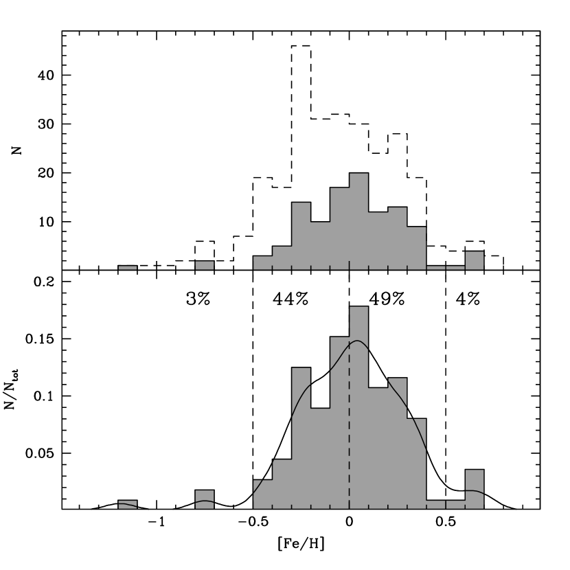
Figure 6: Top panel: Metallicity distribution of the bulge field around Terzan 5 for the entire sample of 284 stars (dashed histogram) and for the sub-set of 112 targets selected at $9.2<K_{c}<9.8$ (grey histogram), free from the bias introduced by the TiO bands (which preferentially affects the spectra of the most metal-rich objects). Bottom panel: Metallicity distribution observed in the unbiased sub-set of stars (the same grey histogram as above), compared to the generalized distribution (solid line) obtained from 1000 realization described in the text (Section 4.5). The dashed lines delimit the metallicity ranges adopted to define the R_l/h parameter (see text). The percentage of stars in each metallicity range is also marked.

The iron abundances and their total uncertainties for each of the 284 targets analyzed are listed in Table 1, together with the adopted atmospheric parameters. The [Fe/H] distribution for the entire sample is shown as a dashed-line histogram in Figure 6. The distribution is quite broad, extending from [Fe/H]$\simeq-1.2$ dex, up to [Fe/H]$\simeq 0.8$ dex, with a pronounced peak at [Fe/H]$=-0.25$ dex. However, the exclusion of a significant fraction of stars with spectra seriously contaminated by TiO bands (see Setc. 4), possibly introduced a selection bias on the derived metallicity distribution. In fact prominent TiO bands are preferentially expected in the coolest and reddest stars. This is indeed confirmed by Figure 5, showing that the targets for which no abundance measure was feasible (open circles) preferentially populate the brightest and coolest portion of the RGB. Since this is also the region were the most metal-rich stars are expected to be found, in order to provide a meaningful metallicity distribution, representative of the bulge population around Terzan 5, we restricted our analysis to a sub-sample of targets likely not affected by such a bias. To this purpose, in the CMD corrected for internal reddening we selected only stars in the magnitude range $9.2<K_{c}<9.8$ (see dashed lines in Figure 5), where metallicity measurements have been possible for 82% of the surveyed stars (i.e., 112 objects over a total of 136). The metallicity distribution for this sub-sample is shown as a grey histogram in the top panel of Figure 6. The distribution is still quite broad, extending from [Fe/H]$\simeq-1.2$ dex up to [Fe/H]$\simeq 0.7$ dex, but the sub-solar component (with $-0.5<$[Fe/H]$<0$ dex) seems to be comparable in size to the super-solar component (with $0<$[Fe/H]$<0.5$ dex).

In order to properly evaluate the existence of any residual bias, we followed the method described in Zoccali et al. (2008). We considered three strips in the CMD roughly parallel to the slope of the bulge RGB (Figure 5). In each strip, we computed the fraction $f$ defined as the ratio between the number of stars with measured metallicity and the number of targets observed in the spectroscopic surveys. In the selected sub-sample, the $f$ parameter ranges from 0.75 up to 0.90, with the peak in the central bin and with the reddest bin being the less sampled. In order to evaluate the impact of this residual inhomogeneity on the derived metallicity distribution we randomly subtracted from the bluest and central bins a number of stars (2 and 18, respectively) suitable to make the $f$ ratio constant in all the strips. We repeated such a procedure $1000$ times, and for each iteration a new metallicity distribution has been computed. The bottom panel of Figure 6 shows the generalized distribution obtained from the entire procedure, overplotted to the observed one. As can be seen, the two distributions are fully compatible, thus providing the final confirmation that the observed distribution is not affected by any substantial residual bias. Hence it has been adopted as representative of the metallicity distribution of the bulge population around Terzan 5.

In order to compare our results with previous studies, in Figure 7 we show the metallicity distribution obtained in the present work and those derived in different regions of the Galactic bulge: $-6$°$<$b$<-2$°(for a sub-sample of micro-lensed dwarfs Bensby et al., 2013), the Baade’s window (for a sub-sample of giants; Hill et al., 2011 and Zoccali et al., 2008), l$=-5.5$°, b$=-7$°(for a sample of giants; Johnson et al., 2013), and the Ness et al. (2013) field closest to the Galactic disk, at b$=-5$°. The distributions appear quite different. However a few common characteristics can be noted and deserve a brief discussion. Apart from the presence of more or less pronounced peaks, all the distributions show: ($i$) a major sub-solar ([Fe/H]$\simeq-0.2$ dex) component; ($ii$) a super-solar component ([Fe/H]$\simeq 0.2$ dex); ($iii$) a quite extended tail towards low metallicities (reaching [Fe/H]$\simeq-1.5$ dex). However, the relative percentage in the two prominent components appears to be different from one field to another. In order to properly quantify this feature, we defined the ratio R${}_{l/h}=$N${}_{l}/$N_h, where N_l is the number of stars in the sub-solar component (with $-0.5<$[Fe/H]$<0$ dex) and N_h is the number of stars in the super-solar component (with $0<$[Fe/H]$<0.5$ dex). The value of R_l/h is labelled in each panel of Figure 7.

In Figure 8 we plot the value of R_l/h for 13 bulge regions at different latitudes published in the literature (see e.g. Bensby et al. 2013, Hill et al. 2011, Zoccali et al. 2008, Johnson et al. 2011, 2013, Gonzalez et al. 2011, Ness et al. 2013). The value obtained for the bulge field around Terzan 5 is shown as a large filled circle. It is interesting to note how the populations observed in the 13 reference fields define a clear trend, suggesting that the super-solar component tends to be dominant at latitudes below $|$b$|<5$°. The field around Terzan 5 is located at the lowest latitude observed so far. It nicely fits into this trend, and it suggests the presence of a plateau at R${}_{l/h}\sim 0.8$ for $|$b$|<4$°(see also Rich et al. 2012). On the other hand, the Galactic location of the field can possibly be the reason for the small amount of stars detected with [Fe/H]$<-0.5$. Figure 9 shows the fraction (f_MP) of metal-poor objects (with [Fe/H]$<-0.5$) with respect to the total number of stars for each of the samples described in Figure 8, as a function of $|$b$|$. Also in this case a clear trend is defined: the percentage of metal-poor stars drops from $\sim 40$% at $|$b$|\sim 10$°  to a few percent at the latitude of Terzan 5, the only exception being the most external field of Zoccali et al. (2008). Our findings are in good agreement with several recent results about the general properties of the Galactic bulge. Indeed, metal-rich stars are dominant at low Galactic latitudes, that is closer to the Galactic plane (see e.g. Ness et al., 2014, and references therein). Also, we checked the impact on these findings of the assumption of a $8$ kpc distance. We repeated the chemical analysis by adopting distances of $6$ and $10$ kpc. The change of the surface gravity (on average $+0.25$ dex and $-0.2$ dex, respectively) leads to only small differences in the measured [Fe/H], with the stellar metallicities differing on average by $0.06$ dex ($\sigma=0.04$ dex) and $-0.05$ dex ($\sigma=0.02$ dex), in the two cases. Such a tiny difference moves the value of R_l/h from $0.89$ to $0.58$ and $1.26$, respectively, leaving it fully compatible with a flat behavior for $|$b$|<4$° in both cases, while it does not change significantly (less than 1%) the value of f_MP. We underline that this is the first determination of the spectroscopic metallicity distribution for a significant sample of stars at these low and positive Galactic latitudes. Other spectroscopic surveys at low latitudes are needed to confirm the existence of these features.

Finally it is worth commenting on the velocity dispersion obtained for the two main metallicity components in the field surrounding Terzan 5. We found two similar values, $\sigma_{v}=108\pm 8$ km s^-1 and $\sigma_{v}=111\pm 11$ km s^-1 for the sub-solar and the super-solar component, respectively. The two measured values are in agreement with those observed in the fields at b$=-5$° and at low longitudes (l$<5$°) by Ness et al. (2013, see the red diamonds in the lower panels of their Figure 7) in the same metallicity range (-0.5$<$[Fe/H]$<0.5$ dex).

5 SUMMARY

We determined the radial velocity distribution for a sample of 615 stars at (l,b)=(3.7°,1.8°), representative of the bulge field population surrounding the peculiar stellar system Terzan 5. We found that the distribution is well fitted by a Gaussian function with $<v_{\rm rad}>=21.0\pm 4.6$ km s^-1 and $\sigma_{v}=113.0\pm 2.7$ km s^-1. Once converted to Galactocentric velocities, these values are in agreement with the determinations obtained in other bulge fields previously investigated. We did not find evidence for the high-velocity sub-component recently identified in Nidever et al. (2012).

Because of the strong contamination of TiO bands, we were able to measure the iron abundance only for a sample of 284 stars (corresponding to $\sim 46\%$ of the entire sample) and we could derive an unbiased metallicity distribution only from a sub-sample of 112 stars with $9.2<K_{c}<9.8$. Statistical checks have been used to demonstrate that this is a bias-free sample representative of the bulge population around Terzan 5. The metallicity distribution turns out to be quite broad with a peak at [Fe/H]$\simeq+0.05$ dex and it follows the general metallicity-latitude trend found in previous studies, with the number of super-solar bulge stars systematically increasing with respect to the number of sub-solar ones for decreasing latitude. Indeed the population ratio between the sub-solar and super solar components (quantified here by the parameter R_l/h) measured around Terzan 5 nicely agrees with that observed in other low latitude bulge fields, possibly suggesting the presence of a plateau for $|$b$|<4$°. Moreover, also the fraction of stars with [Fe/H]$<-0.5$ measured around Terzan 5 fits well into the correlation with $|$b$|$ found from previous studies.

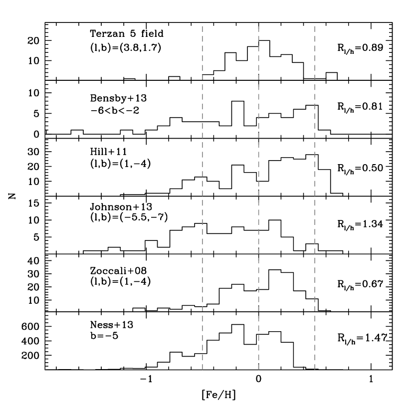
Figure 7: Comparison of the iron distribution in a few bulge fields at different Galactocentric locations. The corresponding references and Galactic coordinates are indicated in each panel. Vertical dashed lines delimitate the metallicity ranges defining the sub- and super-solar metallicity components. The value of the R_l/h parameter defined in the text (Section 4.5) is also reported in each panel.

Figure 8: R_l/h parameter as a function of the Galactic latitude (absolute value). The 13 fields taken from the literature nicely describe a metallicity gradient, suggesting that the super-solar component increases with decreasing Galactic latitude. The field measured around Terzan 5 is highlighted with a large filled circle and possibly suggests the presence of a “plateau” at R${}_{l/h}\simeq 0.8$ for $|$b$|<4$°.

Figure 9: Fraction of metal-poor stars with [Fe/H]$<-0.5$ dex (f_MP) as a function of the absolute value of the Galactic latitude. The considered bulge fields are the same as those in Fig. 8 and also in this case they describe a clear trend, with the only exception of the survey at the largest latitude (from Zoccali et al. 2008). The field measured around Terzan 5 is highlighted with a large filled circle and fits very well into the correlation.

Table 1: Identification number, coordinates, atmospheric parameters, iron abundances and their uncertainties for the Terzan 5 field stars in our sample.

ID	RA	Dec	Teff	log $g$	[Fe/H]	$\sigma_{[Fe/H]}$	Dataset
			(K)	(dex)	(dex)	(dex)
1030711	267.1829348	-24.6923402	3922	0.6	-0.22	0.22	FLAMES
1052484	267.1470436	-24.6830821	4220	0.8	-0.19	0.19	FLAMES
1071029	267.1182806	-24.6825530	3971	1.9	0.39	0.18	FLAMES
1071950	267.1169145	-24.6630493	3832	0.9	0.24	0.19	FLAMES
1072160	267.1165783	-24.6588856	4111	0.9	0.63	0.20	FLAMES
2009060	267.0686838	-24.6638585	4434	0.9	-0.34	0.17	FLAMES
2029939	267.0366131	-24.6637204	4366	1.4	0.69	0.15	FLAMES
2065353	266.9816844	-24.6414183	4013	0.9	-0.04	0.26	FLAMES
2066891	266.9791962	-24.6560448	4371	1.1	0.22	0.19	FLAMES
2068105	266.9771994	-24.6119254	3888	0.9	0.04	0.22	FLAMES

Note. — The entire table is available in the online version of the journal.

References

- Andersen et al. (1999) Andersen, J., et al. 1999, Transactions of the International Astronomical Union, Series A, 24, 36
- Alves-Brito et al. (2010) Alves-Brito, A., Meléndez, J., Asplund, M., Ramírez, I., & Yong, D. 2010, A&A, 513, A35
- Bensby et al. (2013) Bensby, T., Yee, J. C., Feltzing, S., et al. 2013, A&A, 549, A147
- Castelli & Kurucz (2004) Castelli, F., & Kurucz, R. L. 2004, arXiv:astro-ph/0405087
- Carpenter (2001) Carpenter, J. M. 2001, AJ, 121, 2851
- D’Odorico et al. (2006) D’Odorico, S., Dekker, H., Mazzoleni, R., et al. 2006, Proc. SPIE, 6269
- Faber et al. (2003) Faber, S. et al., 2003, SPIE, 4841, 1657
- Ferraro et al. (2009) Ferraro, F. R., Dalessandro, E., Mucciarelli, A., et al. 2009, Nature, 462, 483
- Freeman et al. (2013) Freeman, K., Ness, M., Wylie-de-Boer, E., et al. 2013, MNRAS, 428, 3660
- Fulbright et al. (2007) Fulbright, J. P., McWilliam, A., & Rich, R. M. 2007, ApJ, 661, 1152
- Gonzalez et al. (2011) Gonzalez, O. A., Rejkuba, M., Zoccali, M., et al. 2011, A&A, 530, A54
- Grevesse & Sauval (1998) Grevesse, N. & Sauval, A. J., 1998, SSRv, 85, 161
- Hill et al. (2011) Hill, V., Lecureur, A., Gómez, A., et al. 2011, A&A, 534, A80
- Hinkle et al. (2000) Hinkle, K., Wallace, L., Valenti, J., Harmer, D., 2000, Visible and Near Infrared Atlas of the Arcturus Spectrum 3727-9300 A ed. Kenneth Hinkle, Lloyd Wallace, Jeff Valenti, and Dianne Harmer. (San Francisco: ASP)
- Howard et al. (2008) Howard, C. D., Rich, R. M., Reitzel, D. B., et al. 2008, ApJ, 688, 1060
- Ibata et al. (2011) Ibata, R., Sollima, A., Nipoti, C., Bellazzini, M., Chapman, S. C., & Dalessandro, E., 2011, ApJ, 738, 186
- Johnson et al. (2011) Johnson, C. I., Rich, R. M., Fulbright, J. P., Valenti, E., & McWilliam, A. 2011, ApJ, 732, 108
- Johnson et al. (2013) Johnson, C. I., Rich, R. M., Kobayashi, C., et al. 2013, ApJ, 765, 157
- Kerr & Lynden-Bell (1986) Kerr, F. J., & Lynden-Bell, D. 1986, MNRAS, 221, 1023
- Kunder et al. (2012) Kunder, A., Koch, A., Rich, R. M., et al. 2012, AJ, 143, 57
- Lanzoni et al. (2010) Lanzoni, B., Ferraro, F. R., Dalessandro, E., et al. 2010, ApJ, 717, 653
- Massari et al. (2012) Massari, D., Mucciarelli, A., Dalessandro, E., et al. 2012, ApJ, 755, L32
- McLean et al. (1998) McLean, I. S., Becklin, E. E., Bendiksen, O., et al. 1998, Proc. SPIE, 3354, 566
- McWilliam & Rich (1994) McWilliam, A., & Rich, R. M. 1994, ApJS, 91, 749
- Miocchi et al. (2013) Miocchi, P., Lanzoni, B., Ferraro, F. R., et al. 2013, ApJ, 774, 151
- Montegriffo et al. (1998) Montegriffo, P., Ferraro, F. R., Origlia, L. & Fusi Pecci, F., 1998, MNRAS, 297, 872
- Mucciarelli (2011) Mucciarelli, A., 2011, A&A, 528, 44
- Mucciarelli et al. (2012) Mucciarelli, A., Bellazzini, M., Ibata, R., Merle, T., Chapman, S. C., Dalessandro, E., & Sollima, A., 2012, MNRAS, 426, 2889
- Mucciarelli et al. (2013) Mucciarelli, A., Pancino, E., Lovisi, L., Ferraro, F. R., & Lapenna, E. 2013, ApJ, 766, 78
- Mucciarelli (2013) Mucciarelli, A. 2013, arXiv:1311.1403
- Neckel & Labs (1984) Neckel, H., & Labs, D., 1984, SoPh, 90, 205
- Ness et al. (2013) Ness, M., Freeman, K., Athanassoula, E., et al. 2013, MNRAS, 430, 836
- Ness et al. (2013) Ness, M., Freeman, K., Athanassoula, E., et al. 2013, MNRAS, 432, 2092
- Ness et al. (2014) Ness, M., Debattista, V. P., Bensby, T., et al. 2014, ApJ, 787, L19
- Nidever et al. (2012) Nidever, D. L., Zasowski, G., Majewski, S. R., et al. 2012, ApJ, 755, L25
- Origlia et al. (1997) Origlia, L., Ferraro, F. R., Fusi Pecci, F., & Oliva, E. 1997, A&A, 321, 859
- Origlia et al. (2011) Origlia, L., Rich, R. M., Ferraro, F. R., et al. 2011, ApJ, 726, L20
- Origlia et al. (2013) Origlia, L., Massari, D., Rich, R. M., et al. 2013, arXiv:1311.1706
- Pasquini et al. (2002) Pasquini, L., Avila, G., Blecha, A., et al. 2002, The Messenger, 110, 1
- Ramirez & Allende Prieto (2011) Ramirez, I., & Allende Prieto, C., 2011, ApJ, 743, 135
- Rich et al. (2007) Rich, R. M., Reitzel, D. B., Howard, C. D., & Zhao, H. 2007, ApJ, 658, L29
- Rich et al. (2012) Rich, R. M., Origlia, L., & Valenti, E. 2012, ApJ, 746, 59
- Robin et al. (2003) Robin, A. C., Reylé, C., Derrière, S., & Picaud, S. 2003, A&A, 409, 523ù
- Sbordone et al. (2004) Sbordone, L., Bonifacio, P., Castelli, F., & Kurucz, R. L., MSAIS, 5, 93
- Schönrich et al. (2010) Schönrich, R., Binney, J., & Dehnen, W. 2010, MNRAS, 403, 1829
- Simon & Geha (2007) Simon, J. D., & Geha, M., 2007, ApJ, 670, 313
- Stetson & Pancino (2008) Stetson, P. B., & Pancino, E. 2008, PASP, 120, 1332
- Tonry & Davis (1979) Tonry, J. & Davis, M., 1979, AJ, 84, 1511
- Valenti et al. (2007) Valenti, E., Ferraro, F. R., & Origlia, L. 2007, AJ, 133, 1287
- Valenti et al. (2010) Valenti, E., Ferraro, F. R., & Origlia, L. 2010, MNRAS, 402, 1729
- Zoccali et al. (2008) Zoccali, M., Hill, V., Lecureur, A., et al. 2008, A&A, 486, 177
- Zoccali et al. (2014) Zoccali, M., Gonzalez, O. A., Vasquez, S., et al. 2014, A&A, 562, A66