2014 \jmlrworkshopNeural Connectomics Workshop
Simple connectome inference from partial correlation statistics in calcium imaging
Abstract
In this work, we propose a simple yet effective solution to the problem of connectome inference in calcium imaging data. The proposed algorithm consists of two steps. First, processing the raw signals to detect neural peak activities. Second, inferring the degree of association between neurons from partial correlation statistics. This paper summarises the methodology that led us to win the Connectomics Challenge, proposes a simplified version of our method, and finally compares our results with respect to other inference methods.
keywords:
Connectomics - Network inference - Partial correlation1 Introduction
The human brain is a complex biological organ made of about 100 billion of neurons, each connected to, on average, 7,000 other neurons (Pakkenberg et al., 2003). Unfortunately, direct observation of the connectome, the wiring diagram of the brain, is not yet technically feasible. Without being perfect, calcium imaging currently allows for real-time and simultaneous observation of neuron activity from thousands of neurons, producing individual time-series representing their fluorescence intensity. From these data, the connectome inference problem amounts to retrieving the synaptic connections between neurons on the basis of the fluorescence time-series. This problem is difficult to solve because of experimental issues, including masking effects (i.e., some of the neurons are not observed or confounded with others), the low sampling rate of the optical device with respect to the neural activity speed, or the slow decay of fluorescence.
Formally, the connectome can be represented as a directed graph , where is a set of nodes representing neurons, and is a set of edges representing direct synaptic connections between neurons. Causal interactions are expressed by the direction of edges: indicates that the state of neuron might be caused by the activity of neuron . In those terms, the connectome inference problem is formally stated as follows: Given the sampled observations of neurons for time intervals, the goal is to infer the set of connections in .
In this paper, we present a simplified - and almost as good - version of the winning method111Code available at https://github.com/asutera/kaggle-connectomics of the Connectomics Challenge222http://connectomics.chalearn.org, as a simple and theoretically grounded approach based on signal processing techniques and partial correlation statistics. The paper is structured as follows: Section 2 describes the signal processing methods applied on fluorescent calcium time-series; Section 3 then presents the proposed approach and its theoretical properties; Section 4 provides an empirical analysis and comparison with other network inference methods, while finally, in Section 5 we discuss our work and provide further research directions. Additionally, Appendix A further describes, in full detail, our actual winning method which gives slightly better results than the method presented in this paper, at the cost of parameter tuning. Appendix B provides supplementary results on other datasets.
2 Signal processing
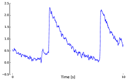
Under the simplifying assumption that neurons are on-off units, characterised by short periods of intense activity, or peaks, and longer periods of inactivity, the first part of our algorithm consists of cleaning the raw fluorescence data. More specifically, time-series are processed using standard signal processing filters in order to : (i) remove noise mainly due to fluctuations independent of calcium, calcium fluctuations independent of spiking activity, calcium fluctuations in nearby tissues that have been mistakenly captured, or simply by the imaging process ; (ii) to account for fluorescence low decay ; and (iii) to reduce the importance of high global activity in the network. The overall process is illustrated in Figure 1.
[Raw signal]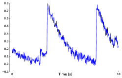 \subfigure[Low-pass filter ]
 \subfigure[High-pass filter ]
\subfigure[Hard-threshold filter ]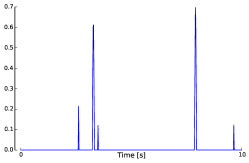 \subfigure[Global regularization ]
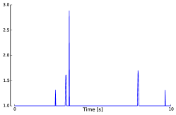
As Figure 1 shows, the raw fluorescence signal is very noisy due to light scattering artifacts that usually affect the quality of the recording (Lichtman and Denk, 2011). Accordingly, the first step of our pipeline is to smoothe the signal, using one of the following low-pass filters for filtering out high frequency noise:
| (1) | ||||
| (2) |
These filters are standard in the signal processing field (Kaiser and Reed, 1977; Oppenheim et al., 1983). For the purposes of illustration, the effect of the filter on the signal is shown in Figure 1.
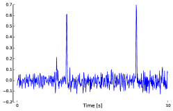
Furthermore, short spikes, characterized by a high frequency, can be seen as an indirect indicator of neuron communication, while low frequencies of the signal mainly correspond to the slow decay of fluorescence. To have a signal that only has high magnitude around instances where the spikes occur, the second step of our pipeline transforms the time-series into its backward difference
| (3) |
as shown in Figure 1.
To filter out small variations in the signal obtained after applying the function , as well as to eliminate negative values, we use the following hard-threshold filter
| (4) |
yielding Figure 1 where is the threshold parameter and is the indicator function. As can be seen, the processed signal only contains clean spikes.
The objective of the last step of our filtering procedure is to decrease the importance of spikes that occur when there is high global activity in the network with respect to spikes that occur during normal activity. Indeed, we have conjectured that when a large part of the network is firing, the rate at which observations are made is not high enough to be able to detect interactions, and that it would therefore be preferable to lower their importance by changing their magnitude appropriately. Additionally, it is well-known that neurons may also spike because of a high global activity (Stetter et al., 2012). In such context, detecting pairwise neuron interactions from the firing activity is meaningless. As such, the signal output by is finally applied to the following function
| (5) |
whose effect is to magnify the importance of spikes that occur in cases of low global activity (measured by ), as observed, for instance, around in Figure 1. Note the particular case where there is no activity, i.e., , is solved by setting .
3 Connectome inference from partial correlation statistics
Our procedure to infer connections between neurons first assumes that the (filtered) fluorescence concentrations of all neurons at each time point can be modelled as a set of random variables that are independently drawn from the same time-invariant joint probability distribution . As a consequence, our inference method does not exploit the time-ordering of the observations (although time-ordering is exploited by the filters).
Given this assumption, we then propose to use as a measure of the strength of the connection between two neurons and , the Partial correlation coefficient between their corresponding random variables and , defined by:
| (6) |
where , known as the precision or concentration matrix, is the inverse of the covariance matrix of . Assuming that the distribution is a multivariate Gaussian distribution , it can be shown that is zero if and only if and are independent given all other variables in , i.e., where . Partial correlation thus measures conditional dependencies between variables ; therefore it should naturally only detect direct associations between neurons and filter out spurious indirect effects. The interest of partial correlation as an association measure has already been shown for the inference of gene regulatory networks (De La Fuente et al., 2004; Schäfer and Strimmer, 2005). Note that the partial correlation statistic is symmetric (i.e. ). Therefore, our approach cannot identify the direction of the interactions between neurons. We will see in Section 4 why this only slightly affects its performance, with respect to the metric used in the Connectomics Challenge.
Practically speaking, the computation of all coefficients using Equation 6 requires the estimation of the covariance matrix and then computing its inverse. Given that typically we have more samples than neurons, the covariance matrix can be inverted in a straightforward way. We nevertheless obtained some improvement by replacing the exact inverse with an approximation using only the first principal components (Bishop, 2006) (with in our experiments, see Appendix C).
Finally, it should be noted that the performance of our simple method appears to be quite sensitive to the values of parameters (e.g., choice of or or the value of the threshold ) in the combined function of the filtering and inferring processes. One approach, further referred to as Averaged Partial correlation statistics, for improving its robustness is to average correlation statistics over various values of the parameters, thereby reducing the variance of its predictions. Further details about parameter selection are provided in Appendix A.
4 Experiments
Data and evaluation metrics.
We report here experiments on the normal-1,2,3, and 4 datasets provided by the organisers of the Connectomics Challenge (see Appendix B for experiments on other datasets). Each of these datasets is obtained from the simulation (Stetter et al., 2012) of different neural networks of 1,000 neurons and approximately 15,000 edges (i.e., a network density of about 1.5%). Each neuron is described by a calcium fluorescence time-series of length . All inference methods compared here provide a ranking of all pairs of neurons according to some association score. To assess the quality of this ranking, we compute both ROC and precision-recall curves against the ground-truth network, which are represented by the area under the curves and respectively denoted AUROC and AUPRC. Only the AUROC score was used to rank the challenge participants, but the precision-recall curve has been shown to be a more sensible metric for network inference, especially when network density is small (see e.g., Schrynemackers et al. (2013)). Since neurons are not self-connected in the ground-truth networks (i.e., ), we have manually set the score of such edges to the minimum possible association score before computing ROC and PR curves.
Evaluation of the method.
The top of Table 1 reports AUROC and AUPRC for all four networks using, in each case, partial correlation with different filtering functions. Except for the last two rows that use PCA, the exact inverse of the covariance matrix was used in each case. These results clearly show the importance of the filters. AUROC increases in average from 0.77 to 0.93. PCA does not really affect AUROC scores, but it significantly improves AUPRC scores. Taking the average over various parameter settings gives an improvement of 10% in AUPRC but only a minor change in AUROC. The last row (“Full method”) shows the final performance of the method specifically tuned for the challenge (see Appendix A for all details). Although this tuning was decisive to obtain the best performance in the challenge, it does not significantly improve either AUROC or AUPRC.
| AUROC | AUPRC | |||||||
| Method normal- | 1 | 2 | 3 | 4 | 1 | 2 | 3 | 4 |
| No filtering | 0.777 | 0.767 | 0.772 | 0.774 | 0.070 | 0.064 | 0.068 | 0.072 |
| 0.923 | 0.925 | 0.923 | 0.922 | 0.311 | 0.315 | 0.313 | 0.304 | |
| 0.931 | 0.929 | 0.928 | 0.926 | 0.326 | 0.323 | 0.319 | 0.303 | |
| + PCA | 0.932 | 0.930 | 0.928 | 0.926 | 0.355 | 0.353 | 0.350 | 0.333 |
| Averaging | 0.937 | 0.935 | 0.935 | 0.931 | 0.391 | 0.390 | 0.385 | 0.375 |
| Full method | 0.943 | 0.942 | 0.942 | 0.939 | 0.403 | 0.404 | 0.398 | 0.388 |
| PC | 0.886 | 0.884 | 0.891 | 0.877 | 0.153 | 0.145 | 0.170 | 0.132 |
| GTE | 0.890 | 0.893 | 0.894 | 0.873 | 0.171 | 0.174 | 0.197 | 0.142 |
| GENIE3 | 0.892 | 0.891 | 0.887 | 0.887 | 0.232 | 0.221 | 0.237 | 0.215 |
Comparison with other methods.
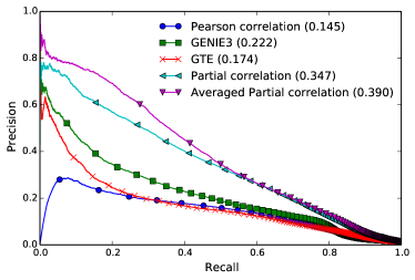
At the bottom of Table 1, we provide as a comparison the performance of three other methods: standard (Pearson) correlation (PC), generalised transfer entropy (GTE), and GENIE3. ROC and PR curves on the normal-2 network are shown for all methods in Figure2. Pearson correlation measures the unconditional linear (in)dependence between variables and it should thus not be able to filter out indirect interactions between neurons. GTE (Stetter et al., 2012) was proposed as a baseline for the challenge. This method builds on Transfer Entropy to measure the association between two neurons. Unlike our approach, it can predict the direction of the edges. GENIE3 (Huynh-Thu et al., 2010) is a gene regulatory network inference method that was the best performer in the DREAM5 challenge (Marbach et al., 2012). When transposed to neural networks, this method uses the importance score of variable in a Random Forest model trying to predict from all variables in as a confidence score for the edge going from neuron to neuron . However, to reduce the computational cost of this method, we had to limit each tree in the Random Forest model to a maximum depth of 3. This constraint has a potentially severe effect on the performance of this method with respect to the use of fully-grown trees. PC and GENIE3 were applied to the time-series filtered using the functions and (which gave the best performance), respectively. For GENIE3, we built 10,000 trees per neuron and we used default settings for all other parameters (except for the maximal tree depth). For GTE, we reproduced the exact same setting (conditioning level and pre-processing) that was used by the organisers of the challenge.
Partial correlation and averaged partial correlation clearly outperform all other methods on all datasets (see Table 1 and Appendix B). The improvement is more important in terms of AUPRC than in terms of AUROC. As expected, Pearson correlation performs very poorly in terms of AUPRC. GTE and GENIE3 work much better, but these two methods are nevertheless clearly below partial correlation. Among these two methods, GTE is slightly better in terms of AUROC, while GENIE3 is significantly better in terms of AUPRC. Given that we had to limit this latter method for computational reasons, these results are very promising and a comparison with the full GENIE3 approach is certainly part of our future works.
The fact that our method is unable to predict edge directions does not seem to be a disadvantage with respect to GTE and GENIE3. Although partial correlation scores each edge, and its opposite, similarly, it can reach precision values higher than 0.5 (see Figure 2(b)), suggesting that it mainly ranks high pairs of neurons that interact in both directions. It is interesting also to note that, on normal-2, a method that perfectly predicts the undirected network (i.e., that gives a score of to each pair such that or , and otherwise) already reaches an AUROC as high as and an AUPRC of .
[ROC curves]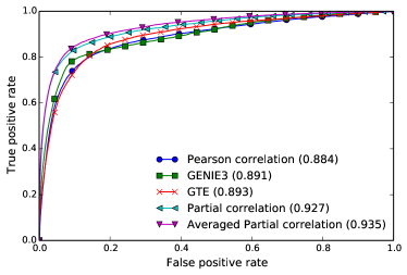 \subfigure[Precision-recall curves]
5 Conclusions
In this paper, we outlined a simple but efficient methodology for the problem of connectome inference from calcium imaging data. Our approach consists of two steps: (i) processing fluorescence data to detect neural peak activities; and (ii) inferring the degree of association between neurons from partial correlation statistics. Its simplified variant outperforms other network inference methods while its optimized version proved to be the best method on the Connectomics Challenge. Given its simplicity and good performance, we therefore believe that the methodology presented in this work would constitute a solid and easily-reproducible baseline for further work in the field of connectome inference.
Acknowledgments
A. Joly and G. Louppe are research fellows of the FNRS, Belgium. A. Sutera is a recipient of an FRIA fellowship of FRS-FNRS, Belgium. This work is supported by PASCAL2 and the IUAP DYSCO, initiated by the Belgian State, Science Policy Office.
References
- Alter et al. (2000) Orly Alter, Patrick O Brown, and David Botstein. Singular value decomposition for genome-wide expression data processing and modeling. Proceedings of the National Academy of Sciences, 97(18):10101–10106, 2000.
- Bishop (2006) Christopher M Bishop. Pattern recognition and machine learning, volume 1. Springer New York, 2006.
- De La Fuente et al. (2004) Alberto De La Fuente, Nan Bing, Ina Hoeschele, and Pedro Mendes. Discovery of meaningful associations in genomic data using partial correlation coefficients. Bioinformatics, 20(18):3565–3574, 2004.
- Huynh-Thu et al. (2010) Vân Anh Huynh-Thu, Alexandre Irrthum, Louis Wehenkel, and Pierre Geurts. Inferring regulatory networks from expression data using tree-based methods. PloS one, 5(9):e12776, 2010.
- Jolliffe (2005) Ian Jolliffe. Principal component analysis. Wiley Online Library, 2005.
- Kaiser and Reed (1977) JF Kaiser and WA Reed. Data smoothing using low-pass digital filters. Review of Scientific Instruments, 48(11):1447–1457, 1977.
- Lichtman and Denk (2011) Jeff W Lichtman and Winfried Denk. The big and the small: challenges of imaging the brain’s circuits. Science, 334(6056):618–623, 2011.
- Marbach et al. (2012) Daniel Marbach, James C. Costello, Robert Küffner, Nicole Vega, Robert J. Prill, Diogo M. Camacho, Kyle R. Allison, The DREAM5 Consortium, Manolis Kellis, James J. Collins, and Gustavo Stolovitzky. Wisdom of crowds for robust network inference. Nature methods, 9(8):794–804, 2012.
- Oppenheim et al. (1983) Alan V Oppenheim, Alan S Willsky, and Syed Hamid Nawab. Signals and systems, volume 2. Prentice-Hall Englewood Cliffs, NJ, 1983.
- Pakkenberg et al. (2003) Bente Pakkenberg, Dorte Pelvig, Lisbeth Marner, Mads J Bundgaard, Hans Jørgen G Gundersen, Jens R Nyengaard, and Lisbeth Regeur. Aging and the human neocortex. Experimental gerontology, 38(1):95–99, 2003.
- Schäfer and Strimmer (2005) Juliane Schäfer and Korbinian Strimmer. A shrinkage approach to large-scale covariance matrix estimation and implications for functional genomics. Statistical applications in genetics and molecular biology, 4(32):1175, 2005.
- Schrynemackers et al. (2013) Marie Schrynemackers, Robert Küffner, and Pierre Geurts. On protocols and measures for the validation of supervised methods for the inference of biological networks. Frontiers in genetics, 4, 2013.
- Stetter et al. (2012) Olav Stetter, Demian Battaglia, Jordi Soriano, and Theo Geisel. Model-free reconstruction of excitatory neuronal connectivity from calcium imaging signals. PLoS computational biology, 8(8):e1002653, 2012.
Appendix A Description of the “Full method”
This section provides a detailed description of the method specifically tuned for the Connectomics Challenge. We restrict our description to the differences with respect to the simplified method presented in the main paper. Most parameters were tuned so as to maximize AUROC on the normal-1 dataset and our design choices were validated by monitoring the AUROC obtained by the 145 entries we submitted during the challenge. Although the tuned method performs better than the simplified one on the challenge dataset, we believe that the tuned method clearly overfits the simulator used to generate the challenge data and that the simplified method should work equally well on new independent datasets. We nevertheless provide the tuned method here for reference purposes. Our implementation of the tuned method is available at https://github.com/asutera/kaggle-connectomics.
This appendix is structured as follows: Section A.1 describes the differences in terms of signal processing. Section A.2 then provides a detailed presentation of the averaging approach. Section A.3 presents an approach to correct the values so as to take into account the edge directionality. Finally, Section A.4 presents some experimental results to validate the different steps of our proposal.
A.1 Signal processing
In Section 2, we introduced four filtering functions (, , , and ) that are composed in sequence (i.e., ) to provide the signals from which to compute partial correlation statistics. Filtering is modified as follows in the tuned method:
- •
-
•
An additional filter is applied to smoothe differences in peak magnitudes that might remain after the application of the hard-threshold filter :
(9) with .
-
•
Filter is replaced by a more complex filter defined as:
(10) where the function is a piecewise linear function optimised separately for each filter , , and (see the implementation for full details). Filter in the simplified method is a special case of with .
The pre-processed time-series are then obtained by the application of the following function: (with , 2, 3, or 4).
A.2 Weighted average of partial correlation statistics
As discussed in Section 3, the performance of the method (in terms of AUROC) is sensitive to the value of the parameter of the hard-threshold filter (see Equation 4), and to the choice of the low-pass filter (among ). As in the simplified method, we have averaged the partial correlation statistics obtained for all the pairs .
Filters and display similar performances and thus were given similar weights (i.e., resp. and ). These weights were chosen equal to the weights selected for the simplified method. In contrast, filters and turn out, individually, to be less competitive and were therefore given less importance in the weighted average (i.e., resp. and ). Yet, as further shown in Section A.4, combining all filters proves to marginally improve performance with respect to using only and .
A.3 Prediction of edge orientation
Partial correlation statistics is a symmetric measure, while the connectome is a directed graph. It could thus be beneficial to try to predict edge orientation. In this section, we present an heuristic that modifies the computed by the approach described before which takes into account directionality.
This approach is based on the following observation. The rise of fluorescence of a neuron indicates its activation. If another neuron is activated after a slight delay, this could be a consequence of the activation of the first neuron and therefore indicates a directed link in the connectome from the first to the second neuron. Given this observation, we have computed the following term for every pair :
| (11) |
that could be interpreted as an image of the number of times that neuron activates neuron . and are parameters whose values have been chosen in our experiments equal to and , respectively. Their role is to define when the difference between and can indeed be assimilated to an event for which neuron activates neuron .
Afterwards, we have computed the difference between and , that we call , and used this difference to modify and so as to take into account directionality. Naturally, if is greater (smaller) than , we may conclude that should there be an edge between and , then this edge would have to be oriented from to ( to ).
This suggests the new association matrix :
| (12) |
where is another parameter. We discovered that this new matrix was not providing good results, probably due to the fact that directivity was not rewarded well enough in the challenge.
This has lead us to investigate other ways for exploiting the information about directionality contained in the matrix . One of those ways that gave good performance was to use as an association matrix:
| (13) |
with chosen close to 1 (). Note that with values for close to 1, matrix only uses the information to a minimum about directivity contained in to modify the partial correlation matrix . We tried smaller values for but those provided poorer results.
A.4 Experiments
On the interest of low-pass filters and .
As reported in Table 2, averaging over all low-pass filters leads to better AUROC scores than averaging over only two low-pass filters, i.e., and . However this slightly reduces AUPRC.
| AUROC | AUPRC | |||||||
|---|---|---|---|---|---|---|---|---|
| Averaging normal- | 1 | 2 | 3 | 4 | 1 | 2 | 3 | 4 |
| with , | 0.937 | 0.935 | 0.935 | 0.931 | 0.391 | 0.390 | 0.385 | 0.375 |
| with , , , | 0.938 | 0.936 | 0.936 | 0.932 | 0.391 | 0.389 | 0.385 | 0.374 |
On the interest of using matrix rather than to take into account directivity.
Table 3 compares AUROC and AUPRC with or without correcting the values according to Equation 13. Both AUROC and AUPRC are (very slightly) improved by using information about directivity.
| AUROC | AUPRC | |||||||
|---|---|---|---|---|---|---|---|---|
| Full method normal- | 1 | 2 | 3 | 4 | 1 | 2 | 3 | 4 |
| Undirected | 0.943 | 0.942 | 0.942 | 0.939 | 0.403 | 0.404 | 0.398 | 0.388 |
| Directed | 0.944 | 0.943 | 0.942 | 0.940 | 0.404 | 0.405 | 0.399 | 0.389 |
Appendix B Supplementary results
In this appendix we report the performance of the different methods compared in the paper on 6 additional datasets provided by the Challenge organisers. These datasets, corresponding each to networks of 1,000 neurons, are similar to the normal datasets except for one feature:
- lowcon:
-
Similar network but on average with a lower number of connections per neuron.
- highcon:
-
Similar network but on average with a higher number of connections per neuron.
- lowcc:
-
Similar network but on average with a lower clustering coefficient.
- highcc:
-
Similar network but on average with a higher clustering coefficient.
- normal-3-highrate:
-
Same topology as normal-3 but with a higher firing frequency, i.e., with highly active neurons.
- normal-4-lownoise:
-
Same topology as normal-4 but with a better signal-to-noise ratio.
The results of several methods applied to these 6 datasets are provided in Table 4. They confirm what we observed on the normal datasets. Average partial correlation and its tuned variant, i.e.,“Full method”, clearly outperform other network inference methods on all datasets. PC is close to GENIE3 and GTE, but still slightly worse. GENIE3 performs better than GTE most of the time. Note that the ”Full method” reported in this table does not use Equation 13 to slightly correct the values of to take into account directivity.
| AUROC | ||||||
| Method normal- | lowcon | highcon | lowcc | highcc | 3-highrate | 4-lownoise |
| Averaging | 0.947 | 0.943 | 0.920 | 0.942 | 0.959 | 0.934 |
| Full method | 0.955 | 0.944 | 0.925 | 0.946 | 0.961 | 0.941 |
| PC | 0.782 | 0.920 | 0.846 | 0.897 | 0.898 | 0.873 |
| GTE | 0.846 | 0.905 | 0.848 | 0.899 | 0.905 | 0.879 |
| GENIE3 | 0.781 | 0.924 | 0.879 | 0.902 | 0.886 | 0.890 |
| AUPRC | ||||||
| Averaging | 0.320 | 0.429 | 0.262 | 0.478 | 0.443 | 0.412 |
| Full method | 0.334 | 0.413 | 0.260 | 0.486 | 0.452 | 0.432 |
| PC | 0.074 | 0.218 | 0.082 | 0.165 | 0.193 | 0.135 |
| GTE | 0.094 | 0.211 | 0.081 | 0.165 | 0.210 | 0.144 |
| GENIE3 | 0.128 | 0.273 | 0.116 | 0.309 | 0.256 | 0.224 |
Appendix C On the selection of the number of principal components
The (true) network, seen as a matrix, can be decomposed through a singular value decomposition (SVD) or principal component analysis (PCA), so as to respectively determine a set of independent linear combinations of the variable (Alter et al., 2000), or a reduced set of linear combinations combine, which then maximize the explained variance of the data (Jolliffe, 2005). Since SVD and PCA are related, they can be defined by the same goal: both aim at finding a reduced set of neurons, known as components, whose activity can explain the rest of the network.
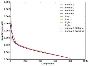
The distribution of compoment eigen values obtained from PCA and SVD decompositions can be studied by sorting them in descending order of magnitude, as illustrated in Figure 3. It can be seen that some component eigen values are zero, implying that the behaviour of the network could be explained by a subset of neurons because of the redundancy and relations between the neurons. For all datasets, the eigen value distribution is exactly the same.
In the context of the challenge, we observe that only components seem to be necessary and we exploit this when computing partial correlation statistics. Therefore, the value of the parameter is immediate and should be clearly set to ().
Note that if the true network is not available, similar decomposition analysis could be carried on the inferred network, or on the data directly.
[PCA]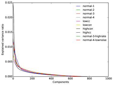 \subfigure[SVD]
Appendix D Summary Table
| Team Name | The AAAGV Team |
|---|---|
| Private leaderboard position | \nth1 |
| Private leaderboard performance | 0.94161 |
| Private leaderboard performance of the winner | idem |