On Minimal Corrections in ASP

Abstract

As a programming paradigm, answer set programming (ASP) brings about the usual issue of the human error. Hence, it is desirable to provide automated techniques that could help the programmer to find the error. This paper addresses the question of computing a subset-minimal correction of a contradictory ASP program. A contradictory ASP program is often undesirable and we wish to provide an automated way of fixing it. We consider a minimal correction set of a contradictory program to be an irreducible set of rules whose removal makes the program consistent. In contrast to propositional logic, corrections of ASP programs behave non-monotonically. Nevertheless, we show that a variety of algorithms for correction set computation in propositional logic can be ported to ASP. An experimental evaluation was carried showing that having a portfolio of such algorithms is indeed of benefit.

1 Introduction

Answer set programming (ASP) is a powerful paradigm for modeling and solving combinatorial and optimization problems in artificial intelligence. An inconsistent program is such a program that does not have a solution. This might be due to a bug in the program and for such cases it is desirable to provide the programmer with tools that would help him to identify the issue.

The primary motivation for this paper is to focus on program’s input. In theory, an input to an ASP program is really just another ASP program that is joined to the original one. In practice, however, the conceptual division between a program and its input plays an important role in the program’s development. Indeed, a program, as a set of rules, expresses the semantics of the problem being solved. The input is a set of facts describing a particular instance of the problem. Such input is typically large.

This paper asks the question, how to resolve situations when there is an error in the given input? In particular, we consider scenarios when the input leads to a contradiction in the program. Consider the following simple program.

$$\leftarrow\operatorname*{\textit{not}\hskip 1.0pt}\operatorname{\textit{move}}(a).$$ % program (1)

$$\operatorname{\textit{move}}(a) \leftarrow\operatorname{\textit{stone}}(b),\operatorname*{\textit{not}\hskip 1.0pt}\operatorname{\textit{stone}}(c).$$ % program (2)

$$\operatorname{\textit{stone}}(c) \leftarrow.$$ % input (3)

By rule (1) the program requires $\operatorname{\textit{move}}(a)$ be true. To achieve that, however, $\operatorname{\textit{stone}}(b)$ must be true and $\operatorname{\textit{stone}}(c)$ must be false (by rule (2)). The input is specified as the fact (3). Altogether, the program is inconsistent since rule (2) is not applicable. If we wish to modify the input so it becomes consistent, the fact $\operatorname{\textit{stone}}(c)$ must be removed and the fact $\operatorname{\textit{stone}}(b)$ must be added. It is the aim of this paper to compute such corrections to inconsistent inputs. Further, we aim at corrections that are irreducible, i.e. that do not perform unnecessary changes. Note that this program could also be made consistent by modifying the rules (1) and (2). Similarly, one could add the fact $\operatorname{\textit{move}}(a)$. This might be undesirable as these represent the rules of the modeled move (in a game, for instance). In the end, however, it is the programmer that must decide what to correct. The objective of the proposed tool-support is to pin-point the source of the inconsistency.

We show that the problem of inconsistency corrections is closely related to a problem of maximal consistency, which we define as identifying a subset-maximal set of atoms that can be added to the program as facts while preserving consistency. Maximal consistency lets us provide a solution to inconsistency correction but it is also an interesting problem to study on its on.

Maximal consistency is closely related to the concept of maximally satisfiable sets (MSS) in propositional logic. For a formula in conjunctive normal form, an MSS is a subset of the formula’s clauses that is satisfiable and adding any clause to it makes it unsatisfiable. There is also a dual, minimal correction subset (MCS), which is a complement of an MSS [18].

There is an important difference between propositional logic and ASP and that is that ASP is not monotone. This means that an algorithm for calculating MSSes cannot be immediately used for ASP. We show, however, that it is possible to port existing MSS algorithms to ASP. This represents a great potential for calculating maximally consistent sets in ASP as a bevy of algorithms for MSS exist [2, 19, 20].

The main contributions of this paper are the following. (1) It devises a technique for adapting algorithms from MSS computation to maximal consistency in ASP. (2) Using the technique a handful of MSS algorithms is adapted to ASP. (3) It is shown how maximal consistency can be used to calculate minimal corrections to ASP inputs. (4) The proposed algorithms were implemented and evaluated on a number of benchmarks.

The paper is organized as follows. Section 3 introduces the concept of maximal consistent subsets and proposes a handful of algorithms for computing them. Section 4 relates maximal consistent subsets to corrections of programs. Section 5 presents experimental evaluation of the presented algorithms. Section 6 briefly overview related work–in ASP but also in propositional logic. Finally, Section 7 concludes and discusses topics of future work.

2 Background

We assume the reader’s familiarity with standard ASP syntax and semantics, e.g. [3]. Here we briefly review the basic notation and concepts. In particular, a (normal) logic program is a finite set of rules of the following form.

$$a\leftarrow b_{1},\dots,b_{m},\operatorname*{\textit{not}\hskip 1.0pt}c_{m+1},\dots,\operatorname*{\textit{not}\hskip 1.0pt}c_{n},$$

where $a,b_{i},c_{j}$ are atoms. A literal is an atom or its default negation $\operatorname*{\textit{not}\hskip 1.0pt}a$. A rule is called a fact if it has an empty body; in such case we don’t write the symbol $\leftarrow$. For a rule $r$, we write $\operatorname{\textit{body}}(r)$ to denote the literals $b_{1},\dots,b_{m},\operatorname*{\textit{not}\hskip 1.0pt}c_{m+1},\dots,\operatorname*{\textit{not}\hskip 1.0pt}c_{n}$ and we write $\operatorname{\textit{head}}(r)$ to denote the literal $a$. We write $B^{+}(r)$ for $b_{1}\dots,_{m}$ and $B^{-}(r)$ for $c_{m+1},\dots,c_{n}$. Further, we allow choice rules of the form

$$n\leq\{a_{1},\dots,a_{k}\}.$$

(this is a special case of weight constraint rules [28, 22, 29]).

A program is called ground if does not contain any variables. A ground instance of a program $P$, denoted as $\operatorname*{\textit{grd}}(P)$, is a ground program obtained by substituting variables of $P$ by all constants from its Herbrand universe.

The semantics of ASP programs can be defined via a reduct [13, 14]. Let $I$ be a set of ground atoms. The set $I$ is a model of a program $P$ if $\operatorname{\textit{head}}(r)\in I$ whenever $B^{+}(r)\subseteq I$ and $B^{-}(r)\cap I=\emptyset$ for every $r\in\operatorname*{\textit{grd}}(P)$. The reduct of a program $P$ w.r.t. the set $I$ is denoted as $P^{I}$ and defined as follows.

$$P^{I}=\left\{{\operatorname{\textit{head}}(r)}\;|\;{r\in\operatorname*{\textit{grd}}(P),I\cap B^{-}(r)=\emptyset}\right\}$$

The set $I$ is an answer set of $P$ if $I$ is a minimal model of $P^{I}$. This definition guarantees that an answer set contains only atoms that have an acyclic justification by the rules of $P$ (cf. [17]). A choice rule $l\leq\{s_{1},\dots,s_{k}\}.$ in a program additionally guarantees that any answer set contains at least $l$ atoms from $s_{1},\dots,s_{k}$, and, the rule provides a justification for any of those atoms. For precise semantics see [22, 29]. A program is consistent if it has at least one answer set, it is inconsistent otherwise.

3 Maximal Consistency in ASP

This section studies the problem of computing a maximal subset of given atoms whose addition to the program, as facts, yields a consistent program.

Definition 1 (maximal consistent subset)

Let $P$ be a consistent ASP program and $\operatorname*{\mathcal{S}}$ be a set of atoms. A set $\operatorname*{\mathcal{L}}\subseteq\operatorname*{\mathcal{S}}$ is a maximal consistent subset of $\operatorname*{\mathcal{S}}$ w.r.t. $P$ if the program $P\operatorname{\cup}\left\{{s.}\;|\;{s\in\operatorname*{\mathcal{L}}}\right\}$ is consistent and for any $\operatorname*{\mathcal{L}}^{\prime}$, such that $\operatorname*{\mathcal{L}}\subsetneq\operatorname*{\mathcal{L}}^{\prime}\subseteq\operatorname*{\mathcal{S}}$, the program $P\operatorname{\cup}\left\{{s.}\;|\;{s\in\operatorname*{\mathcal{L}}^{\prime}}\right\}$ is inconsistent.

The definition of maximal consistent subset is syntactically similar to maximal models or MSSes in propositional logic. Semantically, however, there is an important difference due to nonmonotonicity of ASP. While in propositional logic the satisfiability of $\phi\land x\land y$ guarantees satisfiability of $\phi\land x$, in ASP it is not necessarily the case. Hence, algorithms for MSSes in propositional logic cannot be readily used for our maximal consistent subset. We will show, however, that it is possible to port these algorithms to ASP.

In the following we use some auxiliary functions. The function $\textnormal{{choice}}(\operatorname*{\mathcal{S}})$ produces the choice rule $0\leq\{s_{1},\dots,s_{k}\}$ over the set $\operatorname*{\mathcal{S}}=\{s_{1},\dots,s_{k}\}$. The function $\textnormal{{atleast1}}(\{s_{1},\dots,s_{k}\})$ produces the choice rule $1\leq\{s_{1},\dots,s_{k}\}$. An ASP solver is modeled by the function $\textnormal{{solve}}(P)$, which returns a pair $(\textnormal{{res}},\mu)$ where res is true if and only if $P$ is consistent and $\mu$ is an answer set of $P$ if some exists.

A brute force approach to calculating a maximal consistent subset would be to enumerate all subsets of $\operatorname*{\mathcal{S}}$ and for each test whether it is still consistent. As there are $2^{|\operatorname*{\mathcal{S}}|}$ subsets of $\operatorname*{\mathcal{S}}$, this approach is clearly unfeasible.

A better approach is to maximize the sum $\Sigma_{s\in S}s$ with respect to the program $P$. Such ensures finding a maximal consistent subset with maximum cardinality. This can be done by iteratively calling an ASP solver while imposing increasing cardinality on the set $\operatorname*{\mathcal{S}}$. However, modern ASP solvers directly support minimization constraints through which maximization can be specified by minimizing negation of the atoms in $\operatorname*{\mathcal{S}}$. This approach was taken elsewhere [30, 10].

Finding a maximal correction subset with maximum cardinality might be computationally harder than finding some maximal correction subset. This is the purposed of the rest of the section.

We begin by an important observation that it is possible to check whether a set of atoms $\operatorname*{\mathcal{L}}$ can be extended into a consistent set of atoms by a single call to an ASP solver.

Observation 1

Let $P$ be an ASP program and $\operatorname*{\mathcal{L}}\subseteq\operatorname*{\mathcal{S}}$ be sets of atoms. Let $P^{\prime}$ be defined as follows.

$$P^{\prime}=P\operatorname{\cup}\left\{{s.}\;|\;{s\in\operatorname*{\mathcal{L}}}\right\}\operatorname{\cup}\{\textnormal{{choice}}(\operatorname*{\mathcal{S}}\smallsetminus\operatorname*{\mathcal{L}}).\}$$

There exists a set of atoms $\operatorname*{\mathcal{L}}^{\prime}$ s.t. $\operatorname*{\mathcal{L}}\subseteq\operatorname*{\mathcal{L}}^{\prime}\subseteq\operatorname*{\mathcal{S}}$ iff $P^{\prime}$ has an answer set $\mu$ such that $\operatorname*{\mathcal{L}}^{\prime}=\operatorname*{\mathcal{S}}\cap\mu$.

Observation 1 enables us to check whether a set of atoms can be extended into a consistent set. This is done by letting the solver to chose the additional atoms. Similar reasoning enables us to devise a test for checking that a consistent set $\operatorname*{\mathcal{L}}$ is already maximal. This is done by enforcing that $\operatorname*{\mathcal{L}}$ is extended by at least one element.

Observation 2

Let $P$ be an ASP program and $\operatorname*{\mathcal{S}}$ be a set of atoms. Let $P^{\prime}$ be defined as follows.

$$P^{\prime}=P\operatorname{\cup}\left\{{s.}\;|\;{s\in\operatorname*{\mathcal{L}}}\right\}\operatorname{\cup}\{\textnormal{{atleast1}}(\operatorname*{\mathcal{S}}\smallsetminus\operatorname*{\mathcal{L}})\}$$

A set $\operatorname*{\mathcal{L}}\subseteq\operatorname*{\mathcal{S}}$ is a maximal consistent subset of $\operatorname*{\mathcal{S}}$ iff $P\operatorname{\cup}\left\{{s.}\;|\;{s\in\operatorname*{\mathcal{L}}}\right\}$ is consistent and $P^{\prime}$ is inconsistent.

1 $\operatorname*{\mathcal{L}}\leftarrow\emptyset$

2 while true do

3       $P^{\prime}\leftarrow P\cup\left\{{s.}\;|\;{s\in\operatorname*{\mathcal{L}}}\right\}$

4       $P^{\prime}\leftarrow P^{\prime}\cup\{\textnormal{{atleast1}}(\operatorname*{\mathcal{S}}\smallsetminus\operatorname*{\mathcal{L}}).\}$

5       $(\textnormal{{res}},\mu)\leftarrow\textnormal{{solve}}(P^{\prime})$

6       if $\lnot\textnormal{{res}}$ then return $\operatorname*{\mathcal{L}}$

7       $\operatorname*{\mathcal{L}}\leftarrow\mu\cap\operatorname*{\mathcal{S}}$

8      

Algorithm 1 Atleast-1 algorithm for maximal consistency.

Combining Observation 1 and Observation 2 gives us Algorithm 1. The algorithm maintains a lower bound $\operatorname*{\mathcal{L}}$, which is initialized to the empty set. The set $\operatorname*{\mathcal{L}}$ grows incrementally until a maximal set is found. In each iteration it is tested whether $\operatorname*{\mathcal{L}}$ is already maximal in accord with Observation 2. The invariant of the loop is that the program $P\operatorname{\cup}\left\{{s.}\;|\;{s\in\operatorname*{\mathcal{L}}}\right\}$ is consistent. The set $\operatorname*{\mathcal{L}}$ grows monotonically with the iterations because whenever a new answer set $\mu$ is obtained, it must contain all the atoms from the previous $\operatorname*{\mathcal{L}}$. Hence, the algorithm terminates in at most $|S|$ calls to an ASP solver. Note that the algorithm does not necessarily need all of the $|S|$ iterations since more than one element might be added to $\operatorname*{\mathcal{L}}$ in one iteration. Similar algorithms have been proposed in different contexts, including computing the backbone of a propositional formula [32, 31] and computing an minimal correction set (MCS) of a propositional formula [19].

1 $\operatorname*{\mathcal{L}}\leftarrow\emptyset$

2 while $\operatorname*{\mathcal{S}}\neq\emptyset$ do

3       $s_{f}\leftarrow\text{ pick an arbitrary element from }\operatorname*{\mathcal{S}}$

4       $\operatorname*{\mathcal{S}}\leftarrow\operatorname*{\mathcal{S}}\smallsetminus\{s_{f}\}$

5       $\operatorname*{\mathcal{L}}\leftarrow\operatorname*{\mathcal{L}}\operatorname{\cup}\{s_{f}\}$

6       $P^{\prime}\leftarrow P\operatorname{\cup}\{\textnormal{{choice}}(\operatorname*{\mathcal{S}}).\}$

7       $P^{\prime}\leftarrow P^{\prime}\operatorname{\cup}\left\{{s.}\;|\;{s\in\operatorname*{\mathcal{L}}}\right\}$

8       $(\textnormal{{res}},\mu)\leftarrow\textnormal{{solve}}(P^{\prime})$

9       if $\lnot\textnormal{{res}}$ then $\operatorname*{\mathcal{L}}\leftarrow\operatorname*{\mathcal{L}}\smallsetminus\{s_{f}\}$

10       else $\operatorname*{\mathcal{L}}\leftarrow\mu\cap\operatorname*{\mathcal{S}}$

11      

return $\operatorname*{\mathcal{L}}$

Algorithm 2 Iterative algorithm for maximal consistency.

The second algorithm we propose also maintains a lower bound on a maximal consistent set and tests, one by one, the elements to be added. The pseudo-code can be found in Algorithm 2. In each iteration it tests whether an element $s_{f}$ can be added to the current lower bound $\operatorname*{\mathcal{L}}$. If it is possible, the algorithm continues with a larger $\operatorname*{\mathcal{L}}$. If it not, then $s_{f}$ is removed from $\operatorname*{\mathcal{L}}$ and never inspected again.

In contrast to Algorithm 1, here it is not immediately clear that the returned set is indeed maximal. Indeed, how do we know that if it was impossible to add some element $s_{f}$ to an earlier $\operatorname*{\mathcal{L}}_{1}$, that is it still impossible for the final $\operatorname*{\mathcal{L}}_{f}$? This follows from Observation 1 and from the fact that $\operatorname*{\mathcal{L}}$ grows monotonically throughout the algorithm. More precisely, it holds that $\operatorname*{\mathcal{L}}_{1}\subseteq\operatorname*{\mathcal{L}}_{f}$ and our test checks that $s_{f}$ cannot be added to any superset of $\operatorname*{\mathcal{L}}_{1}$, i.e. if it was not possible to extend $\operatorname*{\mathcal{L}}_{1}$ with $s_{f}$, then it is also impossible to extend $\operatorname*{\mathcal{L}}_{f}$ with it. As Algorithm 1, Algorithm 2 also performs at most $|\operatorname*{\mathcal{S}}|$ calls to an ASP solver. Similar algorithms have been proposed in a number of contexts, including computing an MCS [2, 24].

The third algorithm we consider is inspired by the progression algorithm [20]. The algorithm is shown in Algorithm 3. It tries to add more than a single atom to the lower bound in one iteration—atoms are added in chunks. This is done progressively: in the very first iteration the chunk contains a single atom. The chunk size is doubled each time the current chunk is added with success. If it is not possible to extend the current lower bound $\operatorname*{\mathcal{L}}$ with the current chunk, the size is reset again to $1$. Whenever a chunk of size $1$ cannot be added to $\operatorname*{\mathcal{L}}$ the clause comprising the chunk is no longer inspected. This guarantees termination. Note that the algorithm aims at constructing $\operatorname*{\mathcal{L}}$ as quickly as possible by adding larger chunks of atoms at a time.

$\operatorname*{\mathcal{L}}\leftarrow\emptyset$

  // consistency lower bound

$K\leftarrow 1$

  // chunk size

1 while $\operatorname*{\mathcal{S}}\neq\emptyset$ do

2       $\operatorname*{\mathcal{C}}\leftarrow\text{pick }\textrm{min}(|\operatorname*{\mathcal{S}}|,K)\text{ arbitrary elements from }\operatorname*{\mathcal{S}}$

3       $\operatorname*{\mathcal{S}}\leftarrow\operatorname*{\mathcal{S}}\smallsetminus\operatorname*{\mathcal{C}}$

4       $\operatorname*{\mathcal{L}}\leftarrow\operatorname*{\mathcal{L}}\operatorname{\cup}\operatorname*{\mathcal{C}}$

5       $P^{\prime}\leftarrow P\operatorname{\cup}\{\textnormal{{choice}}(\operatorname*{\mathcal{S}}).\}$

6       $P^{\prime}\leftarrow P^{\prime}\operatorname{\cup}\left\{{s.}\;|\;{s\in\operatorname*{\mathcal{L}}}\right\}$

7       $(\textnormal{{res}},\mu)\leftarrow\textnormal{{solve}}(P^{\prime})$

8       if $\lnot\textnormal{{res}}$ then

            

             // re-analyze chunk more finely

9             $\operatorname*{\mathcal{L}}\leftarrow\operatorname*{\mathcal{L}}\smallsetminus\operatorname*{\mathcal{C}}$

10             if $K>1$ then $\operatorname*{\mathcal{S}}\leftarrow\operatorname*{\mathcal{S}}\operatorname{\cup}\operatorname*{\mathcal{C}}$

             $K=1$

              // reset chunk size

11            

12      else

             $K\leftarrow 2K$

              // double chunk size

             $\operatorname*{\mathcal{L}}\leftarrow\mu\cap\operatorname*{\mathcal{S}}$

              // observe that $\operatorname*{\mathcal{C}}\subseteq(\mu\cap\operatorname*{\mathcal{S}})$

13            

14      

return $\operatorname*{\mathcal{L}}$

Algorithm 3 Progression-based algorithm for maximal consistency.

The use of chunks finds other applications, including redundancy removal [4].

4 From Maximal Consistency to Minimal Corrections

In this section we see how maximal consistency is useful for calculating corrections to an inconsistent program. Hence, the objective is to calculate an irreducible correction to a given inconsistent program so it becomes consistent.

The concept of (minimal) correction sets commonly appears in propositional logic [2]. Correction sets, however, are meant to be removed from the formula in order to make it consistent. In ASP, however, corrections might consist of removal or addition. Indeed, unlike in propositional logic, an ASP program may become consistent after a fact (or rule) is added.

Enabling corrections by addition brings about a substantial difficulty as the universe of rules that can be potentially added to the program can be easily unwieldy or even infinite. Hence, we assume that the user (the programmer) provides us with a set of rules $\operatorname*{\mathcal{R}}$ that can be removed from the program and a set of rules $\operatorname*{\mathcal{A}}$ that can be added to the program.

Definition 2 ($(\operatorname*{\mathcal{A}},\operatorname*{\mathcal{R}})$-correction)

Let $\operatorname*{\mathcal{A}}$ and $\operatorname*{\mathcal{R}}$ be sets of rules and $P$ be an inconsistent logic program. An $(\operatorname*{\mathcal{A}},\operatorname*{\mathcal{R}})$-correction of $P$ is a pair $(M_{r},M_{a})$ such that $M_{r}\subseteq\operatorname*{\mathcal{R}}$ and $M_{a}\subseteq\operatorname*{\mathcal{A}}$ and the program $(P\setminus M_{r})\cup M_{a}$ is consistent.

An $(\operatorname*{\mathcal{A}},\operatorname*{\mathcal{R}})$-correction $(M_{r},M_{a})$ is minimal if for any $(\operatorname*{\mathcal{A}},\operatorname*{\mathcal{R}})$-correction $(M^{\prime}_{r},M^{\prime}_{a})$ such that $M_{r}^{\prime}\subseteq M_{r}$ and $M^{\prime}_{a}\subseteq M_{a}$, it holds that $M_{a}=M^{\prime}_{a}$ and $M_{r}=M^{\prime}_{r}$.

We refer to the problem of calculating a minimal correction as MinCorrect; it accepts as input sets $\operatorname*{\mathcal{A}}$, $\operatorname*{\mathcal{R}}$, and a program $P$ and outputs a pair $(M_{r},M_{a})$ in accord with 2.

We show how to translate MinCorrect to maximal consistent subset calculation. Construct a program $P^{\prime}$ from $P$ as follows.

1. Introduce fresh atoms $s_{r}^{\mathrm{r}}$ for each $r\in\operatorname*{\mathcal{R}}$ and $s_{r}^{\mathrm{a}}$ for each $r\in\operatorname*{\mathcal{A}}$.

2. Replace each rule $r\in\operatorname*{\mathcal{R}}$ with $\operatorname{\textit{head}}(r)\leftarrow s_{r}^{\mathrm{r}},\ \operatorname{\textit{body}}(r)$

3. Replace each rule $r\in\operatorname*{\mathcal{A}}$ with $\operatorname{\textit{head}}(r)\leftarrow\operatorname*{\textit{not}\hskip 1.0pt}s_{r}^{\mathrm{a}},\ \operatorname{\textit{body}}(r)$.

Let $\operatorname*{\mathcal{S}}=\left\{{s_{r}^{\mathrm{r}}}\;|\;{r\in\operatorname*{\mathcal{R}}}\right\}\operatorname{\cup}\left\{{s_{r}^{\mathrm{a}}}\;|\;{r\in\operatorname*{\mathcal{A}}}\right\}$. Then any maximal consistent subset $\operatorname*{\mathcal{L}}$ of $\operatorname*{\mathcal{S}}$ w.r.t. $P^{\prime}$ gives us a solution to MinCorrect by setting $M_{r}=\left\{{r}\;|\;{s_{r}^{\mathrm{r}}\notin\operatorname*{\mathcal{L}}}\right\}$ and $M_{a}=\left\{{r}\;|\;{s_{r}^{\mathrm{a}}\notin\operatorname*{\mathcal{L}}}\right\}$. It is easy to see why that is the case. From the definition of maximal consistent subset, there must be an answer set $\mu$ of the program $P^{\prime}\operatorname{\cup}\left\{{s.}\;|\;{s\in\operatorname*{\mathcal{L}}}\right\}$. If $s_{r}^{\mathrm{r}}\in\mu$ for $r\in\operatorname*{\mathcal{R}}$, then $\mu$ also satisfies the original rule $r$, hence it is not necessary to remove $r$ to achieve consistency. Similarly, if $s_{r}^{\mathrm{a}}\in\mu$, then the body of $\operatorname{\textit{head}}(r)\leftarrow\operatorname*{\textit{not}\hskip 1.0pt}s_{r}^{\mathrm{a}},\ \operatorname{\textit{body}}(r)$ is false, i.e. the rule is ineffective, and therefore it is not necessary to add the rule $r$ to the original program to achieve consistency. Conversely, adding any further $s_{r}^{\mathrm{r}}$ or $s_{r}^{\mathrm{a}}$ to $\mu$ leads to inconsistency due to the definition of maximal consistent subset. Hence, $M_{r}$ and $M_{a}$ defined as above are irreducible.

4.1 Minimal Corrections for Program Inputs

Here we come back to the problem that we used to motivate the paper in introduction, which is to calculate corrections of program’s data so that the program becomes consistent. Hence, we assume that there is a program $P_{e}$— representing the encoding of the problem and a program $P_{d}$—representing data to the encoding, consisting only of facts. Assuming that $P_{e}\operatorname{\cup}P_{d}$ is inconsistent, we wish to identify correction to $P_{d}$ that would make it consistent.

For such, we use the concept of minimal corrections as described above. What is needed is to specify the sets $\operatorname*{\mathcal{R}}$ and $\operatorname*{\mathcal{A}}$. To specify the set $\operatorname*{\mathcal{R}}$, the user just needs to identify facts in the given input that can be removed. This can for instance be done by giving predicate names. Specifying the set $\operatorname*{\mathcal{A}}$ is more challenging because it may comprise facts that do not appear in the program. Hence, we let the user give expressions $E$ of the form $p(A_{1}):t(A_{2})$ where $p$ and $t$ are predicate symbols and $A_{1}$,$A_{2}$ appropriate arguments. The set $\operatorname*{\mathcal{A}}$ is obtained by an additional call to an ASP solver. This call constructs a program $P^{\prime}$ just as above and add the rule $\textnormal{{atleast1}}\left(\left\{{s_{r}^{\mathrm{r}}}\;|\;{r\in\operatorname*{\mathcal{R}}}\right\}\cup\{E_{1},\dots,E_{u}\}\right)$. If this call is successful, the obtained answer set contains facts of the form $p(A_{1})$ that constitute the set $\operatorname*{\mathcal{A}}$.

5 Experimental Evaluation

The proposed algorithms were implemented using the state-of-the-art ASP solver clingo, version 4.2.1. Algorithms 1–3 were implemented as presented, i.e. the ASP solver is invoked repeatedly from a python script. Computing a cardinality-maximal consistent subset was done by a single call to clingo, using the minimization rule syntax ($:\sim$). For readability we refer to the individual approaches by single letters, Algorithm 1–letter a (atleast-1 constraint); Algorithm 2–letter u (unit addition); Algorithm 3–letter p (progression); the maximization approach is denoted by x. The evaluation was carried out on machines with Intel Xeon 5160 3GHz and 4GB of memory. The time limit was set to 1000 seconds and the memory limit to 2GB. The experimental evaluation considers several problems from the 2013 ASP Competition. The following classes were considered.

Solitaire. In the game a single player moves and removes stones from the board according to the rule that a stone can be moved by two squares if that move jumps over another stone; the stone being jumped over is removed (similarly to Checkers). The problem to be solved in the context of this game is to perform $T$ steps given $T$ and an initial configuration. For instance, the problem does not have a solution if the board contains only one stone and at least one move is required to be made.

The size of the board is 7x7 with 2x2-size corners removed, thus comprising 33 squares. The initial configuration of the board is given by the predicates $\operatorname{\textit{empty}}(L)$ and $\operatorname{\textit{full}}(L)$, where $L$ is a square of the board. The set $\operatorname*{\mathcal{R}}$ was specified as containing all the input’s facts using $\operatorname{\textit{empty}}$ and $\operatorname{\textit{full}}$. The set $\operatorname*{\mathcal{A}}$ was specified by the expressions $\operatorname{\textit{empty}}(L)\,:\,\operatorname{\textit{location}}(L)$ and $\operatorname{\textit{full}}(L)\,:\,\operatorname{\textit{location}}(L)$.

To generate unsatisfiable instances of the game, initial board configurations were generated randomly and the parameter $T$ (number of steps) were fixed. We considered $T=12$ and $T=16$; $100$ instances were generated for each $T$ and only inconsistent were considered. This process was repeated for other benchmarks.

Knight tour with holes. The input is a chessboard of size $N\times N$ with $H$ holes. Following the standard chess rules, a knight chess piece must visit all non-hole position of the boards exactly once and return to the initial position (which may be chosen). The objective of correction was to remove as few holes as possible so that the tour is possible. Random hole positions were generated for fixed $N$ and $H$. Instances with $N=8$, $H=4$ and $N=8$, $H=10$ were considered.

Graceful graphs. Given a graph $(V,E)$ the task is to determine whether it is possible to label its vertices with distinct integers in the range $0..|E|$ so that each edge is labeled with the absolute distinct between the labels of its vertices and sot that all edge labels are distinct (such graph is called graceful). The correction, for a given graph that is not graceful, tried to find its subgraph that maintains as many edges as possible (a single-edge graph is graceful). Considered instances were generated with $|V|=10$ and $|E|=50$ and $|V|=30$ and $|E|=20$.

Permutation Pattern Matching. The problem’s input are two permutations $T$ and $P$. The task is to determine whether $T$ contains a subsequence that is order-isomorphic to $P$. For the purpose of correcting we consider $T$ and $P$ so that $P$ is not an order-isomorphic subsequence of $T$ with the objective of adding and removing elements to $P$ so that $P$ satisfies the condition. Considered instances were generated with $|T|=16$ and $|P|=10$ and $|T|=20$ and $|P|=15$.

Family	a	p	u	x	VBS
knight [8,10] (95)	74	75	78	60	80
knight [8,4] (51)	7	13	13	7	14
patterns [16,10] (100)	100	100	100	100	100
patterns [20,15] (100)	100	100	100	100	100
solitaire [12] (18)	18	18	18	17	18
solitaire [14] (16)	12	9	11	4	13
graceful graphs [10,50] (100)	57	75	63	62	83
graceful graphs [30,20] (57)	56	57	57	55	57
total (537)	424	447	440	405	465

Table 1: Number of solved instances for each instance class. The parameters of the class are given in square brackets while total number of the instances in a clause are in parentheses.

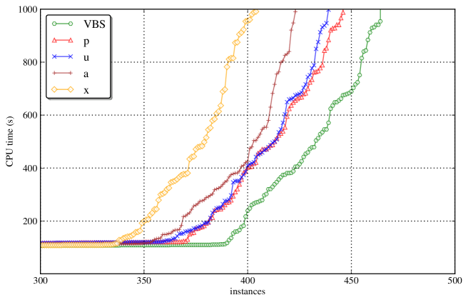
Figure 1: Cactus plot of the overall results where the first 300 easiest instances were cut off. A point in at coordinates $(n,t)$ means that there are $n$ instances such that each is solved in time less than $t$.

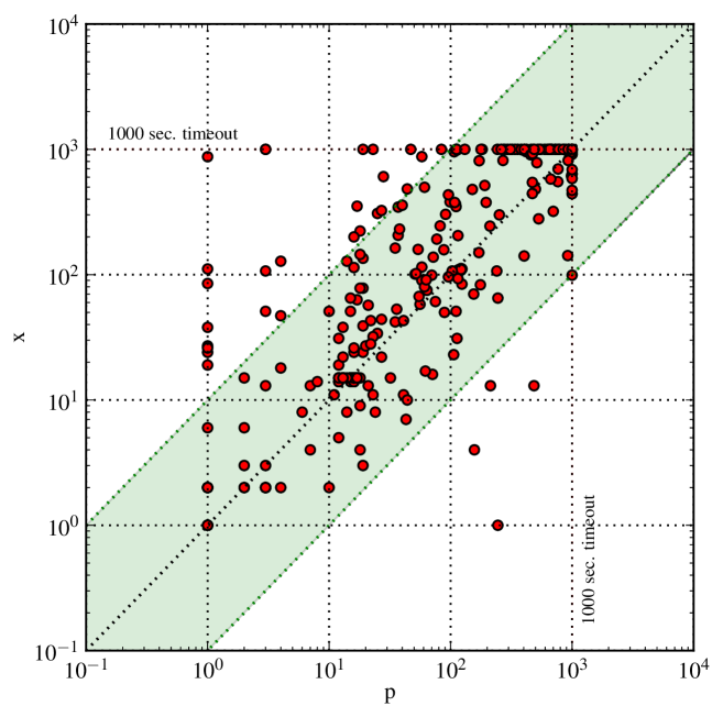
Figure 2: Scatter plot comparing approaches x and p (logarithmic scale).

A more detailed overview of the results can be found on authors’ website. Table 1 shows the number of solved instances by each of the approaches for the different benchmark families. The last column shows the virtual best solver (VBS), which is calculated by picking the best solver for each of the instances. While the progression-based algorithm (p) is clearly in the lead, it is not a winner for all the instances (or even classes of instances). Indeed, the virtual best solver enables us to solve almost 20 more instances compared to the progression-based approach. The strength of progression shows on benchmarks with larger target sets. Such is the case for the class graceful graphs [10,50], where the target set is the set of edges $E$ with $|E|=50$. On the other hand, the approaches a and u do not aim at minimizing the number of calls to the ASP solver but represent calls that are likely to be easier. In u, the solver only must make sure that one fact from the target set is set to true. In a, the solver can in fact chose which fact should be set to true. These algorithms are the two best ones for solitaire [16]. Figure 1 shows a cactus plot across all the considered families (300 easiest instances were cut off for better readability). This plot confirms data in Table 1. Progression provides the most robust solution but at the same time, there is a significant gap between progression and the virtual best solver.

Out of the considered algorithms, cardinality maximization (x) performs the worst. Figure 2 compares progression to cardinality maximization in a scatterplot. There are some instances where maximization performs well but overall progression dominates maximization; by orders of magnitude in a number of cases.

$\mathbf{\Delta}$	a	p	u
0	300	328	332
1	19	16	20
2	38	39	30
3	11	12	14
4	21	16	15
5	8	7	7
6	17	9	8
7	1	1	1
8–20	9	19	13

Table 2: Distribution of how difference between $|M_{a}|+|M_{r}|$ for a–p and for x.

While Algorithms 1–3 give us an advantage over the cardinality maximization approach, the data so far does not show how the minimal corrections differ from the minimum-cardinality corrections in size. This is shown in Table 2. The table shows a distribution of how much the value $|M_{a}|+|M_{r}|$ differs from the value obtained from the approach x. For instance, row 3, column p shows that in 12 cases the value differs by 3 from the minimum one. Naturally, these data only come from instances where x and the given approach finished with success. The distributions have a characteristic “heavy tail”. In the majority of cases , the actual minimum is obtained (over 300 for all the approaches). Outliers exists but they are small in numbers.

6 Related Work

The proposed approach is closely related to the work on debugging on answer set programs [5, 6, 10, 30, 25, 7]. Namely, the approach of Brain et al., which also may produce new facts in a correction [6]. Such facts, however, may only be heads of existing rules. Hence, our approach to data debugging by corrections gives the user a tighter control over the given set of inputs.

Nevertheless, the existing work on ASP debugging (in particular [30, 6, 10]), also needs to deal with removing redundancy. For such, the mentioned works use the cardinality-maximal/minimal sets. Hence, our approach to maximal subset consistency could be applied instead. Our experimental evaluation suggests that this could improve efficiency of those approaches.

Other approaches to maximality in ASP exist. In particular, Gebset et al. [11] use meta-modeling techniques to optimize given criteria and Nieves and Osorio propose calculation of maximal models using ASP [23]. Both approaches, however, hinge on disjunctive logic programming (DLP). Hence, these approaches require solving a problem in the second level of polynomial hierarchy. Intuitively, this means worst-case exponential calls to an NP oracle. In contrast, all our approaches require polynomial calls to an NP oracle.

Some of the algorithms described in the paper are inspired by work on computing MSS/MCSes of propositional formulas in conjunctive normal form, which in term can be traced back to Reiter’s seminal work on model-based diagnosis [27]. The well-known grow procedure is described for example in [2] and more recently in [24]. However, it is used in many other settings, including backbone computation [21] or even prime implicant computation [8]. There has been recent renewed interest in the computation of MCSes [19, 20]. Additional algorithms include the well-known QuickXplain algorithm [16, 9] or dichotomic search [15]. Clearly, and similarly to the case of ASP, MaxSAT can be used for computing and enumerating MCSes [18].

Although the paper considers a restricted sample of algorithms for computing MCS algorithms, adapted from [2, 19, 20], other options would include the additional approaches summarized above.

7 Summary and Future Work

Motivated by debugging of data to ASP programs, the paper studies the problem of minimal (irreducible) corrections of inconsistent programs and the problem of maximal consistency. The two problems are closely related. Indeed, a minimal correction to an inconsistent program can be calculated by computing a maximal consistency with respect to only slightly modified program.

We show that algorithms for calculating maximally satisfiable sets (MSSes) in propositional logic can be adapted to ASP. This is an interesting result as unlike propositional logic, ASP is not monotone. For three MSS algorithms we show how they are ported to ASP (Algorithms 1–3). A similar approach, however, could be used for other MSS algorithms.

The algorithms for maximal consistency let us then calculate minimal corrections. For these corrections we assume a general scheme where rules may be added or removed in order to restore consistency. For evaluation we return to the initial motivation of the paper and that is the calculation of corrections to data that make a program inconsistent. A number of instances from various problem classes were considered. The progression-based algorithm (Algorithm 3) turned out to be the most effective overall. Nevertheless, it was not a winner for each of the considered classes. In contrast, the maximum-cardinality approach clearly performed the worst. Here, however, we should point out that we used the default implementation of minimization in clingo and it is the subject of future work to evaluate other algorithms. (A number of MaxSAT algorithms are being adapted to Max-ASP [26, 1]). Overall, the evaluation suggests that a portfolio comprising the different algorithms would provide the best solution.

The paper opens a number of avenues for future work. Irredundancy is needed in other approaches to debugging, e.g. [30, 6, 10]. It is the subject of future work to evaluate the proposed algorithms also in these contexts. The prototype used for the evaluation uses the ASP solver in a black-box fashion. It is likely that integrating the algorithms directly into an ASP solver would give further performance boost. Similarly, can the proposed algorithms be made more efficient if the algorithms had an access to the workings of the ASP solver?

References

- [1] Andres, B., Kaufmann, B., Matheis, O., Schaub, T.: Unsatisfiability-based optimization in clasp. In: Dovier, A., Costa, V.S. (eds.) ICLP (Technical Communications). LIPIcs, vol. 17, pp. 211–221. Schloss Dagstuhl - Leibniz-Zentrum fuer Informatik (2012)
- [2] Bailey, J., Stuckey, P.J.: Discovery of minimal unsatisfiable subsets of constraints using hitting set dualization. In: PADL (2005)
- [3] Baral, C.: Knowledge representation, reasoning and declarative problem solving. Cambridge University Press (2003)
- [4] Belov, A., Janota, M., Lynce, I., Marques-Silva, J.: On computing minimal equivalent subformulas. In: Milano, M. (ed.) CP. Lecture Notes in Computer Science, vol. 7514, pp. 158–174. Springer (2012)
- [5] Brain, M., De Vos, M.: Debugging logic programs under the answer set semantics. In: ASP Workshop (2005)
- [6] Brain, M.: Declarative problem solving using answer set semantics. In: ICLP. vol. 4079, pp. 459–460 (2006)
- [7] Brummayer, R., Järvisalo, M.: Testing and debugging techniques for answer set solver development. TPLP 10(4-6) (2010)
- [8] Déharbe, D., Fontaine, P., Berre, D.L., Mazure, B.: Computing prime implicants. In: FMCAD. pp. 46–52. IEEE (2013)
- [9] Felfernig, A., Schubert, M., Zehentner, C.: An efficient diagnosis algorithm for inconsistent constraint sets. AI EDAM 26(1), 53–62 (2012)
- [10] Gebser, M., Pührer, J., Schaub, T., Tompits, H.: A meta-programming technique for debugging answer-set programs. In: AAAI (2008)
- [11] Gebser, M., Kaminski, R., Schaub, T.: Complex optimization in answer set programming. TPLP 11(4-5), 821–839 (2011)
- [12] Gelfond, M., Leone, N., Pfeifer, G. (eds.): Logic Programming and Nonmonotonic Reasoning, 5th International Conference, LPNMR’99, El Paso, Texas, USA, December 2-4, 1999, Proceedings, vol. 1730 (1999)
- [13] Gelfond, M., Lifschitz, V.: The stable model semantics for logic programming. In: ICLP/SLP. pp. 1070–1080 (1988)
- [14] Gelfond, M., Lifschitz, V.: Classical negation in logic programs and disjunctive databases. New Generation Comput. 9(3/4), 365–386 (1991)
- [15] Hemery, F., Lecoutre, C., Sais, L., Boussemart, F.: Extracting MUCs from constraint networks. In: Brewka, G., Coradeschi, S., Perini, A., Traverso, P. (eds.) ECAI. Frontiers in Artificial Intelligence and Applications, vol. 141, pp. 113–117. IOS Press (2006)
- [16] Junker, U.: QuickXplain: Preferred explanations and relaxations for over-constrained problems. In: McGuinness, D.L., Ferguson, G. (eds.) AAAI. pp. 167–172. AAAI Press / The MIT Press (2004)
- [17] Lee, J.: A model-theoretic counterpart of loop formulas. In: IJCAI (2005)
- [18] Liffiton, M.H., Sakallah, K.A.: Algorithms for computing minimal unsatisfiable subsets of constraints. J. Autom. Reasoning 40(1), 1–33 (2008)
- [19] Marques-Silva, J., Heras, F., Janota, M., Previti, A., Belov, A.: On computing minimal correction subsets. In: Rossi, F. (ed.) IJCAI. IJCAI/AAAI (2013)
- [20] Marques-Silva, J., Janota, M., Belov, A.: Minimal sets over monotone predicates in Boolean formulae. In: Sharygina, N., Veith, H. (eds.) CAV. pp. 592–607 (2013)
- [21] Marques-Silva, J., Janota, M., Lynce, I.: On computing backbones of propositional theories. In: Coelho, H., Studer, R., Wooldridge, M. (eds.) ECAI. Frontiers in Artificial Intelligence and Applications, vol. 215, pp. 15–20. IOS Press (2010)
- [22] Niemelä, I., Simons, P., Soininen, T.: Stable model semantics of weight constraint rules. In: Gelfond et al. [12], pp. 317–331
- [23] Nieves, J.C., Osorio, M.: Generating maximal models using the stable model semantics. In: Arrazola, J., Parra, P.P., Osorio, M., Zepeda, C. (eds.) LA-NMR. CEUR Workshop Proceedings, vol. 286. CEUR-WS.org (2007)
- [24] Nöhrer, A., Biere, A., Egyed, A.: Managing SAT inconsistencies with HUMUS. In: Eisenecker, U.W., Apel, S., Gnesi, S. (eds.) VaMoS. pp. 83–91. ACM (2012)
- [25] Oetsch, J., Pührer, J., Tompits, H.: Catching the Ouroboros: On debugging non-ground answer-set programs. TPLP 10(4-6) (2010)
- [26] Oikarinen, E., Järvisalo, M.: Max-ASP: Maximum satisfiability of answer set programs. In: Erdem, E., Lin, F., Schaub, T. (eds.) LPNMR. Lecture Notes in Computer Science, vol. 5753, pp. 236–249. Springer (2009)
- [27] Reiter, R.: A theory of diagnosis from first principles. Artif. Intell. 32(1), 57–95 (1987)
- [28] Simons, P.: Extending the stable model semantics with more expressive rules. In: Gelfond et al. [12], pp. 305–316
- [29] Simons, P., Niemelä, I., Soininen, T.: Extending and implementing the stable model semantics. Artif. Intell. 138(1-2), 181–234 (2002)
- [30] Syrjänen, T.: Debugging inconsistent answer set programs. In: Workshop on Nonmonotonic Reasoning (NMR). pp. 77–83 (2006)
- [31] Zhu, C.S., Weissenbacher, G., Malik, S.: Post-silicon fault localisation using maximum satisfiability and backbones. In: Bjesse, P., Slobodová, A. (eds.) FMCAD. pp. 63–66. FMCAD Inc. (2011)
- [32] Zhu, C.S., Weissenbacher, G., Sethi, D., Malik, S.: SAT-based techniques for determining backbones for post-silicon fault localisation. In: Zilic, Z., Shukla, S.K. (eds.) HLDVT. pp. 84–91. IEEE (2011)