UWThPh-2014-16
Mass renormalization in a toy model
with spontaneously broken symmetry

Abstract

We discuss renormalization in a toy model with one fermion field and one real scalar field $\varphi$, featuring a spontaneously broken discrete symmetry which forbids a fermion mass term and a $\varphi^{3}$ term in the Lagrangian. We employ a renormalization scheme which uses the $\overline{\mbox{MS}}$ scheme for the Yukawa and quartic scalar couplings and renormalizes the vacuum expectation value of $\varphi$ by requiring that the one-point function of the shifted field is zero. In this scheme, the tadpole contributions to the fermion and scalar selfenergies are canceled by choice of the renormalization parameter $\delta v$ of the vacuum expectation value. However, $\delta v$ and, therefore, the tadpole contributions reenter the scheme via the mass renormalization of the scalar, in which place they are indispensable for obtaining finiteness. We emphasize that the above renormalization scheme provides a clear formulation of the hierarchy problem and allows a straightforward generalization to an arbitrary number of fermion and scalar fields.

1 Introduction

Our toy model is described by the Lagrangian

$$\mathcal{L}=i\bar{\chi}_{L}\gamma^{\mu}\partial_{\mu}\chi_{L}+\left(\frac{1}{2}\,y\,\chi_{L}^{T}C^{-1}\chi_{L}\varphi+\mbox{H.c.}\right)+\frac{1}{2}\left(\partial_{\mu}\varphi\right)\left(\partial^{\mu}\varphi\right)-V(\varphi)$$ (1)

with the scalar potential

$$V(\varphi)=\frac{1}{2}\mu^{2}\varphi^{2}+\frac{1}{4}\lambda\varphi^{4}.$$ (2)

It contains a real scalar field $\varphi$ and a Majorana fermion field $\chi_{L}$. The symmetry

$$\mathcal{S}:\quad\varphi\to-\varphi,\quad\chi_{L}\to i\chi_{L}$$ (3)

forbids a tree-level mass term of the Majorana fermion and the term $\varphi^{3}$ in the scalar potential. A possible phase in the Yukawa coupling constant $y$ can be absorbed into the field $\chi_{L}$. Therefore, without loss of generality we assume that $y$ is real and positive.

Alternatively, we may consider a Dirac fermion in the toy model. In this case, there are two different chiral fields $\chi_{L}$ and $\chi_{R}$ and the Lagrangian reads

$$\mathcal{L}=i\bar{\chi}_{L}\gamma^{\mu}\partial_{\mu}\chi_{L}+i\bar{\chi}_{R}\gamma^{\mu}\partial_{\mu}\chi_{R}-\left(y\,\bar{\chi}_{L}\chi_{R}\varphi+\mbox{H.c.}\right)+\frac{1}{2}\left(\partial_{\mu}\varphi\right)\left(\partial^{\mu}\varphi\right)-V(\varphi).$$ (4)

The transformation of the fermion field in equation (3) can for instance be modified to $\chi_{L}\to-\chi_{L}$ and $\chi_{R}\to\chi_{R}$, in order to forbid a fermion mass at the tree level.

We will assume $\mu^{2}<0$, which leads to spontaneous symmetry breaking of $\mathcal{S}$ with a tree-level vacuum expectation value (VEV) of $\varphi$ given by

$$v=\sqrt{-\frac{\mu^{2}}{\lambda}}.$$ (5)

The tree-level masses

$$m_{0}=yv\quad\mbox{and}\quad M_{0}^{2}=2\lambda v^{2}$$ (6)

of the fermion and the scalar, respectively, ensue.

We are interested in the mass renormalization of this most simple spontaneously broken toy model because we want to employ a special renormalization scheme which imposes renormalization conditions on the VEV [1] and on the two coupling constants $y$ and $\lambda$, but not on the masses; we want to discuss this scheme in the most simple environment where we do not have to face the complications by gauge theories and propagator mixing. We will explicitly compute the one-loop corrections to equation (6). Our motivation for considering this kind of mass renormalization is the following:

1. Due to the renormalization of the vacuum expectation value and the coupling constants, the fermion and scalar masses must be automatically finite. It is the purpose of these notes to work out how the cancellation of divergences in the masses occurs. In particular, we want to elucidate the role of tadpoles [1, 3] in the context of the scalar mass.

2. At a later time, having in mind renormalizable flavour models for fermion masses and mixing, we intend to extend the model to an arbitrary number of fermion and scalar fields. In this case, there are, in general, more Yukawa couplings than fermion masses and it seems practical to renormalize coupling constants and VEVs instead of masses. A further motivation for such a scheme is given by flavour symmetries which may impose tree-level relations among the VEVs and among the Yukawa couplings and, therefore, also on the masses; such relations will obtain finite corrections at the one-loop level.

The paper is organized as follows. In section 2 we describe the renormalization of the toy model. The one-loop fermion and scalar selfenergies, together with the cancellation of infinities and the corrections to equation (6), are discussed in sections 3 and 4, respectively. Since for simplicity we use the $\overline{\mbox{MS}}$ scheme [4] for the renormalization of both the Yukawa and $\varphi^{4}$-coupling constant, we have a dependence of renormalized quantities on the renormalization scale parameter denoted by $\mathcal{M}$ in our paper, which is worked out in section 5. The conclusions are presented in section 6.

2 Renormalization

Dimensional regularization and renormalization:

In the following, bare quantities carry a subscript $B$. Our starting point is the Lagrangian of equation (1), written in bare fields, the bare coupling constants $y_{B}$, $\lambda_{B}$ and the bare mass parameter $\mu^{2}_{B}$. We confine ourselves to the Majorana case because the treatment of the Dirac case is completely analogous. Renormalization splits the bare Lagrangian into

$$\mathcal{L}_{B}=\mathcal{L}+\delta\mathcal{L},$$ (7)

where $\mathcal{L}$ is the renormalized Lagrangian, written in terms of renormalized quantities, and $\delta\mathcal{L}$ contains the counterterms. The renormalized fields $\chi_{L}$ and $\varphi$ are given by the relations

$$\chi_{LB}=\sqrt{Z_{\chi}}\,\chi_{L},\quad\varphi_{B}=\sqrt{Z_{\varphi}}\,\varphi.$$ (8)

Using dimensional regularization, we are working in $d=4-\varepsilon$ dimensions. As usual, in order to have dimensionless coupling constants $y$ and $\lambda$ in $d$ dimensions, the coupling constants are rescaled by

$$y\to y\,\mathcal{M}^{\varepsilon/2},\quad\lambda\to\lambda\,\mathcal{M}^{\varepsilon}$$ (9)

with an arbitrary mass parameter $\mathcal{M}$. Therefore, the renormalized Lagrangian is identical with that of equation (1), provided that we make the replacement of equation (9). Now it is straightforward to write down the counterterms, subsumed in $\delta\mathcal{L}$:

$$\delta\mathcal{L} = \delta_{\chi}\,i\bar{\chi}_{L}\gamma^{\mu}\partial_{\mu}\chi_{L}+\delta_{\varphi}\frac{1}{2}\left(\partial_{\mu}\varphi\right)\left(\partial^{\mu}\varphi\right)$$ (10)

$$+\left(\frac{1}{2}\,\delta y\mathcal{M}^{\varepsilon/2}\,\chi_{L}^{T}C^{-1}\chi_{L}+\mbox{H.c.}\right)\varphi-\frac{1}{2}\delta\mu^{2}\varphi^{2}-\frac{1}{4}\delta\lambda\mathcal{M}^{\varepsilon}\,\varphi^{4}$$

with

$$\delta_{\chi}=Z_{\chi}-1,\quad\delta_{\varphi}=Z_{\varphi}-1$$ (11)

and

$$\delta\mu^{2} = Z_{\varphi}\,\mu^{2}_{B}-\mu^{2},$$ (12)

$$\delta y\mathcal{M}^{\varepsilon/2} = Z_{\chi}\sqrt{Z_{\varphi}}\,y_{B}-y\mathcal{M}^{\varepsilon/2},$$ (13)

$$\delta\lambda\mathcal{M}^{\varepsilon} = Z_{\varphi}^{2}\,\lambda_{B}-\lambda\mathcal{M}^{\varepsilon}.$$ (14)

Spontaneous symmetry breaking:

After renormalization, we implement spontaneous symmetry breaking by assuming $\mu^{2}<0$ and splitting $\varphi$ into

$$\varphi=v\mathcal{M}^{-\varepsilon/2}+h,$$ (15)

where $v$ is given by equation (5). The factor $\mathcal{M}^{-\varepsilon/2}$ ensures that $v$ has the dimension of a mass. With equation (15), the full Lagrangian reads

$$\mathcal{L}_{B} = i\bar{\chi}_{L}\gamma^{\mu}\partial_{\mu}\chi_{L}+\frac{1}{2}\left(\partial_{\mu}h\right)\left(\partial^{\mu}h\right)$$ (16d)

$$+\left(\frac{1}{2}\,y\mathcal{M}^{\varepsilon/2}\,\chi_{L}^{T}C^{-1}\chi_{L}h+\frac{1}{2}\,m_{0}\,\chi_{L}^{T}C^{-1}\chi_{L}+\mbox{H.c.}\right)$$

$$+\left(\frac{1}{2}\,\delta y\mathcal{M}^{\varepsilon/2}\,\chi_{L}^{T}C^{-1}\chi_{L}h+\frac{1}{2}\,\delta yv\,\chi_{L}^{T}C^{-1}\chi_{L}+\mbox{H.c.}\right)$$

$$+\,\delta_{\chi}i\bar{\chi}_{L}\gamma^{\mu}\partial_{\mu}\chi_{L}+\delta_{\varphi}\frac{1}{2}\left(\partial_{\mu}h\right)\left(\partial^{\mu}h\right)-V-\delta V$$

with

$$V+\delta V = \left(-\frac{1}{4}\lambda v^{4}+\frac{1}{2}\delta\mu^{2}v^{2}+\frac{1}{4}\delta\lambda\,v^{4}\right)\mathcal{M}^{-\varepsilon}$$ (17e)

$$+\left(\delta\mu^{2}v+\delta\lambda\,v^{3}\right)\mathcal{M}^{-\varepsilon/2}h$$

$$+\frac{1}{2}\left(M_{0}^{2}+\delta\mu^{2}+3\,\delta\lambda\,v^{2}\right)h^{2}$$

$$+\left(\lambda v+\delta\lambda\,v\right)\mathcal{M}^{\varepsilon/2}h^{3}$$

$$+\frac{1}{4}\left(\lambda+\delta\lambda\right)\mathcal{M}^{\varepsilon}h^{4}.$$

The terms of the scalar potential, including its counterterms, are listed in equation (17) in ascending powers of $h$. The appearance of a term linear in $h$ is analogous to that of the linear $\sigma$-model [6].

Renormalization conditions:

Here we state the five conditions for fixing the five parameters $\delta y$, $\delta\lambda$, $\delta\mu^{2}$, $\delta_{\chi}$ and $\delta_{\varphi}$ in the counterterms.

1. For simplicity, the $\overline{\mathrm{MS}}$ prescription is used to determine $\delta y$ and $\delta\lambda$, i.e. the term proportional to

   $$c_{\infty}=\frac{2}{\varepsilon}-\gamma+\ln(4\pi)$$ (18)

   is subtracted from the fermion vertex and the scalar four-point function, respectively.

2. The term linear in $h$, equation (17e), induces a scalar VEV, i.e. a contribution to the scalar one-point function. We choose $\delta\mu^{2}$ in such a way that the one-point function of the scalar field $h$ vanishes.

3. The wave-function renormalization constants $\delta_{\chi}$ and $\delta_{\varphi}$ are determined such that the residua of the fermion and scalar propagators, respectively, are both one.

As stressed in the introduction, we want to renormalize the VEV, so we have to switch from $\delta\mu^{2}$ to $\delta v$. Of course, this procedure makes only sense in the broken phase of the model. Notice that in general we can define $\delta v$ via

$$v_{B}=\sqrt{-\frac{\mu^{2}_{B}}{\lambda_{B}}},\quad v=\sqrt{-\frac{\mu^{2}}{\lambda}}\quad\mbox{and}\quad\delta v\mathcal{M}^{-\varepsilon/2}=Z_{\varphi}^{-1/2}v_{B}-v\mathcal{M}^{-\varepsilon/2},$$ (19)

in analogy to $\delta y$ and $\delta\lambda$. Starting from $v_{B}$ above, with $\mu^{2}_{B}$ and $\lambda_{B}$ from equations (12) and (14), respectively, we obtain

$$\delta v=v\sqrt{\frac{1+\delta\mu^{2}/\mu^{2}}{1+\delta\lambda/\lambda}}-v,$$ (20)

which allows us to trade $\delta\mu^{2}$ for $\delta v$.

At lowest order, equation (20) yields

$$\delta v=-\frac{1}{M_{0}^{2}}\left(\delta\mu^{2}v+\delta\lambda\,v^{3}\right).$$ (21)

Using this equation to replace $\delta\mu^{2}$ by $\delta v$, the counterterms linear and quadratic in $h$, i.e. equations (17e) and (17e), respectively, assume the form

$$-M_{0}^{2}\,\delta v\mathcal{M}^{-\varepsilon/2}\,h+\frac{1}{2}\left(-2\lambda v\,\delta v+2\delta\lambda\,v^{2}\right)h^{2}.$$ (22)

At one-loop order, there are two tadpole contributions to the scalar one-point function, namely a fermionic contribution $T_{\chi}$ and a scalar contribution $T_{h}$. Thus the associated renormalization condition is [1, 6, 7]

$$\raisebox{-17.07164pt}{\includegraphics[width=11.9501pt,angle={0}]{delta_v.eps}}\;\;+\raisebox{-17.07164pt}{\includegraphics[width=28.45274pt,angle={0}]{fermionic_tadpole.eps}}+\raisebox{-17.07164pt}{\includegraphics[width=28.45274pt,angle={0}]{scalar_tadpole.eps}}=\delta v\mathcal{M}^{-\varepsilon/2}+T_{\chi}+T_{h}=0,$$ (23)

with the fermion and scalar contributions given by

$$T_{\chi} = -\frac{2y\varsigma}{16\pi^{2}}\mathcal{M}^{-\varepsilon/2}\,\frac{m_{0}^{3}}{M_{0}^{2}}\left(c_{\infty}+1-\ln\frac{m_{0}^{2}}{\mathcal{M}^{2}}\right),$$ (24a)

$$T_{h} = \hphantom{-}\frac{3\lambda}{16\pi^{2}}\mathcal{M}^{-\varepsilon/2}\,v\left(c_{\infty}+1-\ln\frac{M_{0}^{2}}{\mathcal{M}^{2}}\right),$$ (24b)

respectively, where $\varsigma$ is defined as

$$\varsigma=\left\{\begin{array}[]{cl}1&\mbox{for a Majorana fermion loop,}\\ 2&\mbox{for a Dirac fermion loop.}\end{array}\right.$$ (25)

The first contribution to equation (23) stems from the counterterm linear in $h$ in equation (22).

Mass parameters:

It is useful to summarize the mass parameters occurring in the model.

• Mass scale of dimensional regularization: $\mathcal{M}$.

• Mass squared of the scalar: $M^{2}=M_{0}^{2}+M_{1}^{2}$, where $M_{0}^{2}=2\lambda v^{2}$ is the tree-level mass squared and $M_{1}^{2}$ the one-loop correction.

• Mass of the fermion: $m=m_{0}+m_{1}$, with the tree level mass $m_{0}=yv$ and its one-loop correction $m_{1}$.

Notes on Feynman rules for Majorana fermions:

The Yukawa interaction term in equation (16d) can be reformulated as

$$\frac{1}{2}\,\chi_{L}^{T}C^{-1}\chi_{L}(v\mathcal{M}^{-\varepsilon/2}+h)+\mbox{H.c.}=-\frac{1}{2}\,\bar{\chi}\chi(v\mathcal{M}^{-\varepsilon/2}+h)\quad\mbox{with}\quad\chi=\chi_{L}+(\chi_{L})^{c},$$ (26)

with the charge conjugation indicated by the superscript. For simplicity we have left out $y\mathcal{M}^{\varepsilon/2}$. Since in a Wick contraction a field $\chi$ can be contracted with both Majorana fermion fields of the Yukawa interaction vertex, the factor $1/2$ in equation (26) is always canceled when the fermion line is not closed. However, with our convention for the Yukawa interaction, in every closed fermion loop one factor $1/2$ remains [5].

Note that for a Dirac fermion field $\chi$ we have defined the Yukawa coupling without the factor $1/2$. Therefore, with our convention there is no difference between the Majorana and Dirac case for fermion lines which are not closed. However, a closed loop of a Dirac fermion does not have a factor $1/2$ in this convention. Therefore, in order to unify the treatment of Majorana and Dirac fermions, we have introduced a factor $\varsigma$ defined in equation (25).

3 Fermion selfenergy

The terms contributing to the renormalized fermion selfenergy at one-loop order are

$$\Sigma(p)=\Sigma_{\mbox{\scriptsize 1-loop}}(p)-\delta_{\chi}\,\not{p}+\delta_{m}^{(\chi)}+y\left\{\delta v+\mathcal{M}^{\varepsilon/2}\left(T_{\chi}+T_{h}\right)\right\}$$ (27)

with

$$\delta_{m}^{(\chi)}=v\,\delta y.$$ (28)

The one-loop contribution is

$$\Sigma_{\mbox{\scriptsize 1-loop}}(p)=\frac{y^{2}}{16\pi^{2}}\left[-c_{\infty}\left(\frac{1}{2}\not{p}+m_{0}\right)+\int_{0}^{1}\mathrm{d}x\left(x\not{p}+m_{0}\right)\ln\frac{\Delta(p^{2})}{\mathcal{M}^{2}}\right]$$ (29)

with

$$\Delta(p^{2})=xM_{0}^{2}+(1-x)m_{0}^{2}-x(1-x)p^{2}.$$ (30)

Due to the renormalization condition (23), the last term in $\Sigma(p)$ vanishes.

The renormalized fermion selfenergy has the structure

$$\Sigma(p)=A(p^{2})\not{p}+B(p^{2})m.$$ (31)

Both $A$ and $B$ are dimensionless and must be finite. Obviously, $A$ can be made finite by an appropriate choice of $\delta_{\chi}$, but for $B$ we do not have such a freedom because

$$\delta y=\frac{y^{3}}{16\pi^{2}}\,c_{\infty}$$ (32)

is already determined by the renormalization of the fermion vertex. Therefore, consistency requires that $\delta_{m}^{(\chi)}$ of equation (28) with this $\delta y$ makes $B$ finite, which is indeed the case.

As emphasized before, in our renormalization scheme the masses are no free parameters but calculable in terms of the parameters of the model. Therefore, imposing the condition of residue one at the pole of the fermion propagator [8],

$$A(m^{2})+2m^{2}\left[A^{\prime}(m^{2})+B^{\prime}(m^{2})\right]=0,$$ (33a)

automatically leads to a formula for the determination of the pole mass:

$$m=m_{0}+m\left[A(m^{2})+B(m^{2})\right].$$ (33b)

In equation (33a), the prime indicates the derivative with respect to $p^{2}$. Since we are satisfied with a one-loop computation, we can replace $m$ by $m_{0}$ in equation (33a) and on the right-hand side of equation (33b). Equation (33a) determines $\delta_{\chi}$ as

$$\delta_{\chi}=\frac{y^{2}}{16\pi^{2}}\left[-\frac{1}{2}c_{\infty}+\int_{0}^{1}\mathrm{d}x\,x\ln\frac{\Delta(m_{0}^{2})}{\mathcal{M}^{2}}-2m_{0}^{2}\int_{0}^{1}\mathrm{d}x\,\frac{x(1-x^{2})}{\Delta(m_{0}^{2})}\right].$$ (34)

Finally, with this $\delta_{\chi}$ and using equation (33b) we obtain

$$m=m_{0}+m_{1}=m_{0}\left[1+\frac{y^{2}}{16\pi^{2}}\left(2m_{0}^{2}\int_{0}^{1}\mathrm{d}x\,\frac{x(1-x^{2})}{\Delta(m_{0}^{2})}+\int_{0}^{1}\mathrm{d}x\ln\frac{\Delta(m_{0}^{2})}{\mathcal{M}^{2}}\right)\right]$$ (35a)

with

$$\Delta(m_{0}^{2})=xM_{0}^{2}+(1-x)^{2}m_{0}^{2}.$$ (35b)

In equation (35a) $m_{1}$ denotes the one-loop mass.

4 Scalar selfenergy

The scalar selfenergy consists of the terms

$$\Pi(p^{2})=\Pi_{\mbox{\scriptsize 1-loop}}(p^{2})-p^{2}\delta_{\varphi}+\delta_{m}^{(h)}+6\lambda v\left\{\delta v+\mathcal{M}^{\varepsilon/2}\left(T_{\chi}+T_{h}\right)\right\}.$$ (36)

Just as for the fermionic selfenergy, the tadpole contributions are canceled by $\delta v$. According to equation (22), the quantity $\delta_{m}^{(h)}$ is given by

$$\delta_{m}^{(h)}=-2\lambda v\,\delta v+2\delta\lambda\,v^{2}.$$ (37)

The one-loop contribution has three terms,

$$\Pi_{\mbox{\scriptsize 1-loop}}(p^{2})=\Pi_{\mbox{\scriptsize 1-loop}}^{(a)}(p^{2})+\Pi_{\mbox{\scriptsize 1-loop}}^{(b)}(p^{2})+\Pi_{\mbox{\scriptsize 1-loop}}^{(c)}(p^{2}),$$ (38)

referring to loops induced by the interaction terms of equations (16d), (17e) and (17e), respectively. The corresponding Feynman diagrams are shown in figure 1.

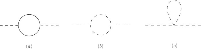
Figure 1: The Feynman diagrams of the three one-loop contributions to the scalar selfenergy.

The results of the one-loop computation are

$$\Pi_{\mbox{\scriptsize 1-loop}}^{(a)}(p^{2}) = \frac{2y^{2}\varsigma}{16\pi^{2}}\int_{0}^{1}\mathrm{d}x\,\Delta_{f}(p^{2})\left(3c_{\infty}+1-3\ln\frac{\Delta_{f}(p^{2})}{\mathcal{M}^{2}}\right),$$ (39a)

$$\Pi_{\mbox{\scriptsize 1-loop}}^{(b)}(p^{2}) = -\frac{9\lambda}{16\pi^{2}}M_{0}^{2}\left(c_{\infty}-\int_{0}^{1}\mathrm{d}x\ln\frac{\Delta_{s}(p^{2})}{\mathcal{M}^{2}}\right),$$ (39b)

$$\Pi_{\mbox{\scriptsize 1-loop}}^{(c)}(p^{2}) = -\frac{3\lambda}{16\pi^{2}}M_{0}^{2}\left(c_{\infty}+1-\ln\frac{M_{0}^{2}}{\mathcal{M}^{2}}\right),$$ (39c)

with

$$\Delta_{f}(p^{2})=m_{0}^{2}-x(1-x)p^{2}\quad\mbox{and}\quad\Delta_{s}(p^{2})=M_{0}^{2}-x(1-x)p^{2}.$$ (40)

In $\delta_{m}^{(h)}$ the counterterm for the quartic scalar coupling is required. It is obtained from the scalar four-point function as

$$\delta\lambda=\frac{1}{16\pi^{2}}c_{\infty}\left(9\lambda^{2}-2\varsigma y^{4}\right).$$ (41)

The renormalized scalar propagator has residue one at the physical mass $M^{2}$ and the physical mass is determined by its pole. This means that the selfenergy has to fulfill

$$\Pi^{\prime}(M^{2})=0\quad\mbox{and}\quad M^{2}=M_{0}^{2}+\Pi(M^{2}),$$ (42)

where the prime indicates the derivative with respect to $p^{2}$. Since we perform a one-loop computation, we can replace $M^{2}$ in both $\Pi^{\prime}(M^{2})$ and $\Pi(M^{2})$ by $M_{0}^{2}$. Thus we find

$$\delta_{\varphi}=\Pi^{\prime}_{\mbox{\scriptsize 1-loop}}(M_{0}^{2})\quad\mbox{and}\quad M^{2}=M_{0}^{2}+M_{1}^{2}\quad\mbox{with}\quad M_{1}^{2}=\Pi(M_{0}^{2}).$$ (43)

Explicitly, $\delta_{\varphi}$ is given by

$$\delta_{\varphi}=\frac{2y^{2}\varsigma}{16\pi^{2}}\int_{0}^{1}\mathrm{d}x\,x(1-x)\left(-3c_{\infty}+2+3\ln\frac{\Delta_{f}(M_{0}^{2})}{\mathcal{M}^{2}}\right)-\frac{9\lambda}{16\pi^{2}}\int_{0}^{1}\mathrm{d}x\,\frac{x(1-x)}{1-x(1-x)}.$$ (44)

On the one hand, the finiteness in the derivative of $\Pi(p^{2})$ has been enforced by the choice of $\delta_{\varphi}$. Actually, only in $\Pi_{\mbox{\scriptsize 1-loop}}^{(a)}(p^{2})$ there is a divergent term proportional to $p^{2}c_{\infty}$ which is eliminated by a corresponding term in $p^{2}\delta_{\varphi}$, the other two contributions ($j=b,c$) to the scalar selfenergy have no such term. On the other hand, for the mass $M_{1}^{2}$ we have no free counterterm anymore and this mass has to be finite via $\delta_{m}^{(h)}$ which we have already determined earlier. Let us denote the $p^{2}$-independent terms proportional to $c_{\infty}$ in $\Pi_{\mbox{\scriptsize 1-loop}}^{(j)}(p^{2})$ by $\Pi^{(j)}_{\infty}$ ($j=a,b,c$). These quantities can be read off from equations (39a), (39b) and (39c), respectively:

$$\Pi^{(a)}_{\infty}=\frac{6y^{2}\varsigma}{16\pi^{2}}m_{0}^{2}c_{\infty},\quad\Pi^{(b)}_{\infty}=-\frac{9\lambda}{16\pi^{2}}M_{0}^{2}c_{\infty},\quad\Pi^{(c)}_{\infty}=-\frac{3\lambda}{16\pi^{2}}M_{0}^{2}c_{\infty}.$$ (45)

The terms proportional to $c_{\infty}$ in $\delta_{m}^{(h)}$ are found by considering equations (24) and (41):

$$(\delta_{m}^{(h)})_{\infty}=\frac{1}{16\pi^{2}}\left[-2\lambda v\left(2y\varsigma\frac{m_{0}^{3}}{M_{0}^{2}}-3\lambda v\right)+2v^{2}\left(9\lambda^{2}-2y^{4}\varsigma\right)\right]c_{\infty}.$$ (46)

It is then easy to check that

$$\sum_{j=a,b,c}\Pi^{(j)}_{\infty}+(\delta_{m}^{(h)})_{\infty}=0.$$ (47)

We stress that, though due to the renormalization condition the tadpole diagrams are canceled by $\delta v$ in the scalar selfenergy, they nevertheless play a crucial role in the cancellation of the infinities in $M_{1}^{2}$ because they occur in the counterterm $\delta_{m}^{(h)}$.

Collecting all terms, we obtain at one-loop order

$$M^{2} = M_{0}^{2}\left\{1-\frac{y^{2}\varsigma}{16\pi^{2}}\left(1+6\frac{m_{0}^{2}}{M_{0}^{2}}\int_{0}^{1}\mathrm{d}x\,\ln\frac{\Delta_{f}(M_{0}^{2})}{\mathcal{M}^{2}}-2\frac{m_{0}^{2}}{M_{0}^{2}}\ln\frac{m_{0}^{2}}{\mathcal{M}^{2}}\right)\right.$$ (48)

$$\left.\hphantom{xxxxx}+\frac{9\lambda}{16\pi^{2}}\left(\ln\frac{M_{0}^{2}}{\mathcal{M}^{2}}-3+\frac{5\pi}{3\sqrt{3}}\right)\right\}.$$

5 $\mathcal{M}$-independence of the particle masses

The one-loop masses $m_{1}$ and $M_{1}^{2}$ depend explicitly on $\mathcal{M}$. However, the fermion and scalar masses, defined as pole masses, are physical observables and have to be independent of $\mathcal{M}$. Since we have performed a one-loop computation, independence means that the $\mathcal{M}$-dependence must cancel at one-loop order which implies that the implicit dependence of $m_{0}$ on $\mathcal{M}$ must be canceled by the explicit dependence of $m_{1}$ on $\mathcal{M}$. The same has to hold for $M_{0}^{2}$ and $M_{1}^{2}$. In the following we will demonstrate this and derive as well some useful other relations concerning the $\mathcal{M}$-dependence. The point of departure is the relationship between bare and renormalized quantities and their counterterms [9]:

$$y_{B} = \mathcal{M}^{\varepsilon/2}\left(y+\delta y\right)Z_{\chi}^{-1}Z_{\varphi}^{-1/2},$$ (49a)

$$\lambda_{B} = \mathcal{M}^{\varepsilon}\left(\lambda+\delta\lambda\right)Z_{\varphi}^{-2},$$ (49b)

$$v_{B} = \mathcal{M}^{-\varepsilon/2}\left(v+\delta v\right)Z_{\varphi}^{1/2}.$$ (49c)

Exploiting the fact that we do not go beyond one-loop order, we obtain from equation (49) formulae for the bare masses:

$$\hphantom{2}y_{B}v_{B}=\left(y+\delta y\right)\left(v+\delta v\right)Z_{\chi}^{-1}=m_{0}\left(1-\delta_{\chi}+\frac{\delta y}{y}+\frac{\delta v}{v}\right),$$ (50)

$$2\lambda_{B}v_{B}^{2}=2\left(\lambda+\delta\lambda\right)\left(v+\delta v\right)^{2}Z_{\varphi}^{-1}=M_{0}^{2}\left(1-\delta_{\varphi}+\frac{\delta\lambda}{\lambda}+2\frac{\delta v}{v}\right).$$ (51)

Takin the derivative of the above equations with respect to $\mathcal{M}$ and taking into account that bare quantities do not depend on $\mathcal{M}$, we arrive at

$$0 = \mathcal{M}\frac{\partial m_{0}}{\partial\mathcal{M}}+m_{0}\,\mathcal{M}\frac{\partial}{\partial\mathcal{M}}\left(-\delta_{\chi}+\frac{\delta y}{y}+\frac{\delta v}{v}\right),$$ (52)

$$0 = \mathcal{M}\frac{\partial M_{0}^{2}}{\partial\mathcal{M}}+M_{0}^{2}\,\mathcal{M}\frac{\partial}{\partial\mathcal{M}}\left(-\delta_{\varphi}+\frac{\delta\lambda}{\lambda}+2\frac{\delta v}{v}\right).$$ (53)

To proceed further we bear in mind that $y^{2}$ and $\lambda$ correspond to the same order in the loop expansion and that from equations (49a) and (49b) we obtain at lowest order $\mathcal{M}\frac{\partial y}{\partial\mathcal{M}}=-\varepsilon y/2+\mathcal{O}(y^{3})$ and $\mathcal{M}\frac{\partial\lambda}{\partial\mathcal{M}}=-\varepsilon\lambda+\mathcal{O}(\lambda^{2})$. Then, with the results of sections 3 and 4, it is straightforward to derive, at order $y^{2}$,

$$\mathcal{M}\frac{\partial}{\partial\mathcal{M}}\delta_{\chi}=\mathcal{M}\frac{\partial}{\partial\mathcal{M}}\delta_{\varphi}=\mathcal{M}\frac{\partial}{\partial\mathcal{M}}\frac{\delta v}{v}=0$$ (54)

and

$$\mathcal{M}\frac{\partial}{\partial\mathcal{M}}\frac{\delta y}{y}=-\frac{2y^{2}}{16\pi^{2}},\quad\mathcal{M}\frac{\partial}{\partial\mathcal{M}}\frac{\delta\lambda}{\lambda}=\frac{1}{16\pi^{2}}\left(-18\lambda+4\varsigma\,\frac{y^{4}}{\lambda}\right).$$ (55)

Plugging these results into equations (52) and (53), we find the implicit dependence of the tree-level masses on $\mathcal{M}$:

$$\mathcal{M}\frac{\partial m_{0}}{\partial\mathcal{M}} = \frac{2y^{2}}{16\pi^{2}}\,m_{0},$$ (56a)

$$\mathcal{M}\frac{\partial M_{0}^{2}}{\partial\mathcal{M}} = \frac{1}{16\pi^{2}}\left(18\lambda M_{0}^{2}-8\varsigma y^{2}m_{0}^{2}\right).$$ (56b)

The latter expression is, of course, proportional to $\delta\lambda$ of equation (41). With equation (56), it is now trivial to see that the derivative of $m_{1}$, equation (35a), and of $M_{1}^{2}$, equation (48), with respect to the explicit dependence on $\mathcal{M}$ leads to expressions with signs opposite to those of equations (56a) and (56b), respectively. Therefore, $m$ and $M^{2}$ are independent of $\mathcal{M}$ at order $y^{2}$ and $\lambda$, which proves our statement in the beginning of this section.

Finally, for completeness we also present the beta functions of $y$, $\lambda$ [10] and $v$ at one-loop order:

$$\mathcal{M}\frac{\partial y}{\partial\mathcal{M}}=-\frac{\varepsilon}{2}\,y+\frac{2y^{3}}{16\pi^{2}},\quad\mathcal{M}\frac{\partial\lambda}{\partial\mathcal{M}}=-\varepsilon\lambda+\frac{1}{16\pi^{2}}\left(18\lambda^{2}-4\varsigma y^{4}\right),\quad\mathcal{M}\frac{\partial v}{\partial\mathcal{M}}=\frac{\varepsilon}{2}\,v.$$ (57)

6 Conclusions

In this paper we have discussed renormalization in a minimalist model with a spontaneously broken discrete symmetry. We have employed a renormalization scheme for the broken phase which renormalizes the VEV such that the one-point function of the shifted field $h$ defined in equation (15) vanishes; for simplicity we have renormalized the Yukawa coupling constant $y$ and the quartic scalar coupling constant $\lambda$ by the $\overline{\mbox{MS}}$ scheme. The renormalization condition for the VEV implies that tadpole contributions to the selfenergies are canceled by the renormalization parameter $\delta v$ of the VEV. In this model, since there is no fermion mass term in the unbroken Lagrangian, it is obvious that the one-loop fermion mass gets renormalized by the renormalization parameter $\delta y$. Concerning the scalar mass, the mass counterterm of the scalar contains explicitly the tadpole contributions in $\delta_{m}^{(h)}$—see equation (37), therefore, both $\delta v$ and $\delta\lambda$ are needed for the finiteness of the scalar mass $M^{2}$. Moreover, $M^{2}$ also receives a finite tadpole contribution.

We have considered this toy model, which does neither have the complications due to gauge interactions [12] nor those due to propagator mixing [13], in view of a future application to renormalizable flavour models. We emphasize that our renormalization scheme has the virtue of facilitating a clear formulation of the hierarchy or fine-tuning problem because it allows the comparison of the tree-level masses with their radiative corrections without obfuscation by a cut-off. In addition, it seems straightforward to extend the model to the case of an arbitrary number of fermion and scalar fields. Finally, we mention that there is an interesting difference between the Majorana and Dirac fermion contribution to the one-loop mass of equation (48) due to occurrence of $\varsigma$—see equation (25) for its definition.

Acknowledgments: This work is supported by the Austrian Science Fund (FWF), Project No. P 24161-N16. W.G. thanks Christoph Bobeth and Martin Gorbahn for discussions on the VEV renormalization during the Workshop “Towards the Construction of the Fundamental Theory of Flavour” at the Institute for Advanced Study TUM in Munich.

References

- [1] J. Fleischer and F. Jegerlehner, Radiative corrections to Higgs decays in the extended Weinberg-Salam Model, Phys. Rev. D 23 (1981) 2001.
-
[2]
N. Cabibbo, L. Maiani, G. Parisi and R. Petronzio,
Bounds on the fermions and Higgs boson masses in grand unified
theories,
Nucl. Phys. B 158 (1979) 295;
E. Ma and S. Pakvasa, Variation of mixing angles and masses with in the standard six quark model, Phys. Rev. D 20 (1979) 2899;
K. Inoue, A. Kakuto and Y. Nakano, Radiative corrections for Yukawa couplings and masses of leptons and quarks in grand unified model, Prog. Theor. Phys. 62 (1979) 307;
W. Grimus, Renormalization group equations of the Salam-Weinberg model and masses of the fermions, Lett. Nuovo Cim. 27 (1980) 169;
B. Pendleton and G. G. Ross, Mass and mixing angle predictions from infrared fixed points, Phys. Lett. B 98 (1981) 291;
M. K. Parida and B. Purkayastha, New formulas and predictions for running masses at higher scales in MSSM, Eur. Phys. J. C 14 (2000) 159 [hep-ph/9902374];
C. R. Das and M. K. Parida, New formulas and predictions for running fermion masses at higher scales in SM, 2 HDM, and MSSM, Eur. Phys. J. C 20 (2001) 121 [hep-ph/0010004]. - [3] S. Weinberg, Perturbative calculations of symmetry breaking, Phys. Rev. D 7 (1973) 2887.
- [4] W. A. Bardeen, A. J. Buras, D. W. Duke and T. Muta, Deep inelastic scattering beyond the leading order in asymptotically free gauge theories, Phys. Rev. D 18 (1978) 3998.
- [5] A. Denner, H. Eck, O. Hahn and J. Küblbeck, Compact Feynman rules for Majorana fermions, Phys. Lett. B 291 (1992) 278.
-
[6]
B. W. Lee,
Renormalization of the -model,
Nucl. Phys. B 9 (1969) 649;
J. L. Gervais and B. W. Lee, Renormalization of the -model (II) Fermion fields and regularization, Nucl. Phys. B 12 (1969) 627. - [7] M. E. Peskin and D. V. Schroeder, An Introduction to Quantum Field theory (Addison-Wesley, Reading 1995).
- [8] K. I. Aoki, Z. Hioki, M. Konuma, R. Kawabe and T. Muta, Electroweak theory. Framework of on-shell renormalization and study of higher order effects, Prog. Theor. Phys. Suppl. 73 (1982) 1.
- [9] J. Collins, Renormalization (Cambridge University Press, 1984).
- [10] T. P. Cheng, E. Eichten and L.-F. Li, Higgs phenomena in asymptotically free gauge theories, Phys. Rev. D 9 (1974) 2259.
- [11] F. Jegerlehner, M. Yu. Kalmykov and B. A. Kniehl, On the difference between the pole and the masses of the top quark at the electroweak scale, Phys. Lett. B 722 (2013) 123 [arXiv:1212.4319 [hep-ph]].
- [12] M. Sperling, D. Stöckinger and A. Voigt, Renormalization of vacuum expectation values in spontaneously broken gauge theories, JHEP 1307 (2013) 132 [arXiv:1305.1548 [hep-ph]].
-
[13]
B. A. Kniehl and A. Pilaftsis,
Mixing renormalization in Majorana neutrino theories,
Nucl. Phys. B 474 (1996) 286
[hep-ph/9601390];
B. A. Kniehl, Propagator mixing renormalization for Majorana fermions, Phys. Rev. D 89 (2014) 116010 [arXiv:1404.5908 [hep-th]].