Conformal Geometry of Sequential Test in Multidimensional Curved Exponential Family

Masayuki Kumon111 Association for Promoting Quality Assurance in Statistics, Tokyo, Japan
Akimichi Takemura 222 Graduate School of Information Science and Technology, University of Tokyo, Tokyo, Japan
Kei Takeuchi 333 Emeritus, Graduate School of Economics, University of Tokyo, Tokyo, Japan
(June 2014)
Abstract

This article presents a differential geometrical method for analyzing sequential test procedures. It is based on the primal result on the conformal geometry of statistical manifold developed in Kumon, Takemura and Takeuchi (2011). By introducing curvature-type random variables, the condition is first clarified for a statistical manifold to be an exponential family under an appropriate sequential test procedure. This result is further elaborated for investigating the efficient sequential test in a multidimensional curved exponential family. The theoretical results are numerically examined by using von Mises-Fisher and hyperboloid models.

Keywords: Curved exponential family; Dual affine connections; Euler-Schouten curvature; Hyperboloid distribution; Information geometry; Riemannian metric; Riemann-Christoffel curvature; Totally umbilic manifold; von Mises-Fisher distribution.

Subject Classifications: 62L12.

1 INTRODUCTION

Sequential inferential procedure continues observations until the observed sample satisfies a certain prescribed criterion. Its properties have been shown to be superior on the average to those of nonsequential inferential procedure in which the number of observations is fixed a priori. Among others Takeuchi and Akahira (1988), Akahira and Takeuchi (1989) formulated the higher-order asymptotic theory of sequential estimation procedures rigorously and analyzed the higher-order efficiency of these procedures in the scalar parameter case. They showed that the exponential curvature term in the second-order variance can be eliminated by the sequential maximum likelihood estimator with the best stopping rule.

Okamoto, Amari and Takeuchi (1991) generalized these works to the multiparameter case by using geometrical notions, and studied characteristics of more general sequential estimation procedures. As indicated there, a sequential estimation procedure with an adequate stopping rule causes a nonuniform expansion of a statistical manifold (Riemannian manifold with a dual couple of affine connections) which is called the conformal transformation. The result of Takeuchi and Akahira can be interpreted such that it is possible to reduce the exponential curvature of a statistical manifold to zero by a suitable conformal transformation. The conformal geometry of statistical manifold thus can be an adequate framework for the analysis of the sequential inferential procedures.

Kumon, Takemura and Takeuchi (2011) conducted this scheme for investigating the sequential estimating procedures from the information geometrical viewpoint. The dual conformal Weyl-Schouten curvature quantity of a statistical manifold was introduced there, and this quantity was proved to play a central role when considering the problem of covariance minimization under the sequential estimating procedures.

This article continues the scheme for investigating the sequential test procedures. We focus on the powers of sequential tests, and pursue the possibility of uniformly efficient (most powerful) sequential test. Different from the previous work, we first introduce the dual Euler-Schouten curvature random variables, and directly study their transformations under the sequential test procedures. These enable us to clarify the condition for a statistical manifold to be an exponential family under an adequate sequential test procedure. We then elaborate the result for analyzing the structure of the uniformly efficient sequential test in a multidimensional curved exponential family. The above approach is motivated by the fact that the exponentiality of a statistical manifold ensures the uniformly efficient inferential procedures in the nonsequential case as well as in the sequential case. Information geometry has been steadily producing mathematical methodologies for a variety of statistical sciences (see e.g., Amari, 1985; Amari et al., 1987; Amari and Nagaoka, 2000; Kumon, 2009, 2010). The present article also is situated in these developments.

The organization of the article is as follows. The established known results are cited as propositions, and the results obtained in this article are stated as theorems. In Section 2, we prepare some statistical notations and preliminary results on the sequential test procedures which will be relevant in this article. In Section 3, we formulate the conformal transformation of statistical manifold, where the dual Euler-Schouten curvature tensor variables are introduced. The related notion of totally exponential umbilic is proved to give the criterion for determining that a statistical manifold can be an exponential family under an suitable sequential test procedure. Its relation to the dual conformal flatness is also explained. In Section 4, we summarize the asymptotics on the nonsequential test in a multidimensional curved exponential family, which are already developed in Kumon and Amari (1983), and Amari (1985, Chapter 6). In Section 5, the general result in Section 3 is used to write down the structure of multidimensional curved exponential family under the sequential test procedures, where the meanings of the dual Euler-Schouten curvatures of statistical submanifold are clarified. In Section 6, we formulate the asymptotics of the sequential test in a multidimensional curved exponential family in line with the nonsequential case, and give the concrete condition and procedure for the uniformly efficient sequential test. In Section 7, the results in Section 6 and also in Section 4 are examined numerically by using two curved exponential families, the von Mises-Fisher model and the hyperboloid model, both of which admit the uniformly efficient sequential test. Section 8 is devoted to some additional discussions and a perspective of future work.

2 PRELIMINARIES

We denote by {X(t)=[X1(t),,Xk(t)]t|tT}conditional-set𝑋𝑡superscriptsubscript𝑋1𝑡subscript𝑋𝑘𝑡t𝑡𝑇\{X(t)=[X_{1}(t),\dots,X_{k}(t)]^{{}^{\mathrm{t}}}\ |\ t\in T\} a k𝑘k-dimensional random sequence defined on the probability space [Ω,,P]Ω𝑃[\Omega,{\cal F},P] with values in [E,]𝐸[E,\cal{E}], where E=k𝐸superscript𝑘E=\mathbb{R}^{k} and \cal{E} is the σ𝜎\sigma-field of all Borel sets in E𝐸E. The time parameter tT𝑡𝑇t\in T runs over all positive integers T={1,2,}𝑇12T=\{1,2,\dots\}. Moreover, let n,nTsubscript𝑛𝑛𝑇{\cal F}_{n},n\in T denote the σ𝜎\sigma-field generated by the n𝑛n-tuple of random vectors Xn=[X(1),,X(n)]superscript𝑋𝑛𝑋1𝑋𝑛X^{n}=[X(1),\dots,X(n)].

In this article, we assume that the probability measure P𝑃P depends on an unknown parameter θ=(θ1,,θm)tΘ𝜃superscriptsuperscript𝜃1superscript𝜃𝑚tΘ\theta=(\theta^{1},\dots,\theta^{m})^{{}^{\mathrm{t}}}\in\Theta, P=Pθ𝑃subscript𝑃𝜃P=P_{\theta}, where ΘΘ\Theta is homeomorphic to msuperscript𝑚{\mathbb{R}}^{m}, and we shall consider the case where the following conditions are fulfilled:

  1. (i)

    The random sequence {X(t)|tT}conditional-set𝑋𝑡𝑡𝑇\{X(t)\ |\ t\in T\} consists of independent and identically distributed k𝑘k-dimensional random variables X(1),X(2),𝑋1𝑋2X(1),X(2),\dots.

  2. (ii)

    The probability distribution of X(1)𝑋1X(1) is dominated by a σ𝜎\sigma-finite measure μ𝜇\mu and has the density f(x,θ)𝑓𝑥𝜃f(x,\theta) with respect to μ𝜇\mu

    dPθdμ(x)=f(x,θ),xE,θΘ,formulae-sequence𝑑subscript𝑃𝜃𝑑𝜇𝑥𝑓𝑥𝜃formulae-sequence𝑥𝐸𝜃Θ\displaystyle\frac{dP_{\theta}}{d\mu}(x)=f(x,\theta),\quad x\in E,\ \theta\in\Theta, (2.1)

    so that the joint density f(xn,n,θ)𝑓superscript𝑥𝑛𝑛𝜃f(x^{n},n,\theta) of Xn=[X(1),,X(n)]superscript𝑋𝑛𝑋1𝑋𝑛X^{n}=[X(1),\dots,X(n)] is written as

    f(xn,n,θ)=t=1nf(x(t),θ),xnEn,θΘ.formulae-sequence𝑓superscript𝑥𝑛𝑛𝜃superscriptsubscriptproduct𝑡1𝑛𝑓𝑥𝑡𝜃formulae-sequencesuperscript𝑥𝑛superscript𝐸𝑛𝜃Θ\displaystyle f(x^{n},n,\theta)=\prod_{t=1}^{n}f(x(t),\theta),\quad x^{n}\in E^{n},\ \theta\in\Theta. (2.2)

We say that {Pθ|θΘ}conditional-setsubscript𝑃𝜃𝜃Θ\{P_{\theta}\ |\ \theta\in\Theta\} is an m𝑚m-dimensional full regular minimally represented exponential family (f.r.m. exponential family) when the density (2.1) can be written as

fe(x,θ)=exp{θixiψ(θ)},subscript𝑓𝑒𝑥𝜃superscript𝜃𝑖subscript𝑥𝑖𝜓𝜃\displaystyle f_{e}(x,\theta)=\exp\{\theta^{i}x_{i}-\psi(\theta)\}, (2.3)

where x=(x1,,xm)tm𝑥superscriptsubscript𝑥1subscript𝑥𝑚tsuperscript𝑚x=(x_{1},\dots,x_{m})^{{}^{\mathrm{t}}}\in{\mathbb{R}}^{m} is the canonical statistic, θ𝜃\theta is the natural parameter, and η=ψ(θ)/θ𝜂𝜓𝜃𝜃\eta=\partial\psi(\theta)/\partial\theta is the expectation parameter with ψ(θ)𝜓𝜃\psi(\theta) a smooth (infinitely differentiable) convex function of θ𝜃\theta. In the right-hand side of (2.3) and hereafter the Einstein summation convention will be assumed, so that summation will be automatically taken over indices repeated twice in the sense, for example, θixi=i=1mθixisuperscript𝜃𝑖subscript𝑥𝑖superscriptsubscript𝑖1𝑚superscript𝜃𝑖subscript𝑥𝑖\theta^{i}x_{i}=\sum_{i=1}^{m}\theta^{i}x_{i}.

Sequential inferential procedures are characterized by a random sample size, where stopping times are used to stop the observations of the process. We denote by τ𝜏\tau an arbitrary stopping time; that is, a random variable τ𝜏\tau defined on ΩΩ\Omega with values in T{}𝑇T\cup\{\infty\} and possessing the property {ωΩ:τ(ω)n}n,nTformulae-sequenceconditional-set𝜔Ω𝜏𝜔𝑛subscript𝑛for-all𝑛𝑇\{\omega\in\Omega:\tau(\omega)\leqslant n\}\in{\cal F}_{n},\ \forall n\in T. This article treats the case to which the Sudakov lemma applies, where the stopped sequence {(Xτ,τ)|τT}conditional-setsuperscript𝑋𝜏𝜏𝜏𝑇\{(X^{\tau},\tau)\ |\ \tau\in T\cup\infty\} has the density f¯(xn,n,θ)¯𝑓superscript𝑥𝑛𝑛𝜃{\bar{f}}(x^{n},n,\theta), and this can be regarded as the same function in (2.2) (cf. e.g., Magiera, 1974).

As a typical statistical problem suppose that we wish to test a simple null hypothesis

H0:θ=θ0ΘvsH1:θθ0.\displaystyle H_{0}:\theta=\theta_{0}\in\Theta\quad\textrm{vs}\quad H_{1}:\theta\neq\theta_{0}.

A sequential test procedure will be based on a test statistic Ynsubscript𝑌𝑛Y_{n} and a stopping time τcn1subscript𝜏𝑐subscript𝑛1\tau_{c}\wedge n_{1}, where

τc=min{nn0:Yn>c},subscript𝜏𝑐:𝑛subscript𝑛0subscript𝑌𝑛𝑐\displaystyle\tau_{c}=\min\{n\geq n_{0}:Y_{n}>c\}, (2.4)

if τcn1subscript𝜏𝑐subscript𝑛1\tau_{c}\leq n_{1}, H0subscript𝐻0H_{0} should be rejected, whereas if τc>n1subscript𝜏𝑐subscript𝑛1\tau_{c}>n_{1}, H0subscript𝐻0H_{0} should not be rejected. Here n0subscript𝑛0n_{0} denotes a given initial sample size and n1subscript𝑛1n_{1} denotes some given maximal sample size. Specifically we take the stopping time τcn1subscript𝜏𝑐subscript𝑛1\tau_{c}\wedge n_{1} with

τc=min{nn0:Yn=ny(X¯n)>ca(n)},X¯n=1nt=1nX(t),formulae-sequencesubscript𝜏𝑐:𝑛subscript𝑛0subscript𝑌𝑛𝑛𝑦subscript¯𝑋𝑛𝑐𝑎𝑛subscript¯𝑋𝑛1𝑛superscriptsubscript𝑡1𝑛𝑋𝑡\displaystyle\tau_{c}=\min\{n\geq n_{0}:Y_{n}=n\cdot y(\bar{X}_{n})>ca(n)\},\quad\bar{X}_{n}=\frac{1}{n}\sum_{t=1}^{n}X(t), (2.5)

where y𝑦y and a𝑎a belong to the following classes of functions 𝒴𝒴\mathcal{Y} and 𝒜𝒜\mathcal{A}, respectively.

Definition 2.1.

The function y(η)𝒴𝑦𝜂𝒴y(\eta)\in{\cal Y} if y(η)𝑦𝜂y(\eta) is positive and smooth in ηk𝜂superscript𝑘\eta\in{\mathbb{R}}^{k}.

Definition 2.2.

The function a(u)𝒜𝑎𝑢𝒜a(u)\in{\cal A} if a(u)𝑎𝑢a(u) is nondecreasing, concave, smooth in uA0𝑢𝐴0u\geq\exists A\geq 0 and regularly varying at infinity with exponent β(0β<1)𝛽0𝛽1\beta\ (0\leq\beta<1) (see Gut, 2009, Appendix B).

Let νc=νc(η)subscript𝜈𝑐subscript𝜈𝑐𝜂\nu_{c}=\nu_{c}(\eta) be the solution of the equation

νcy(η)=ca(νc).subscript𝜈𝑐𝑦𝜂𝑐𝑎subscript𝜈𝑐\displaystyle\nu_{c}y(\eta)=ca(\nu_{c}).

In particular, if a(u)=uβ𝑎𝑢superscript𝑢𝛽a(u)=u^{\beta} for some β(0β<1)𝛽0𝛽1\beta\ (0\leq\beta<1), then νc=(c/y(η))1/(1β)subscript𝜈𝑐superscript𝑐𝑦𝜂11𝛽\nu_{c}=(c/y(\eta))^{1/(1-\beta)}. For β=0𝛽0\beta=0, that is, a(u)1𝑎𝑢1a(u)\equiv 1 and y(η)=|c0+ciηi|𝑦𝜂superscript𝑐0superscript𝑐𝑖subscript𝜂𝑖y(\eta)=|c^{0}+c^{i}\eta_{i}|, the relation reduces to νc=c/|c0+ciηi|subscript𝜈𝑐𝑐superscript𝑐0superscript𝑐𝑖subscript𝜂𝑖\nu_{c}=c/|c^{0}+c^{i}\eta_{i}|.

The above class of stopping times τcsubscript𝜏𝑐\tau_{c} is denoted by 𝒞𝒞{\cal C}. The following is the central limit theorem for a stopping time τc𝒞subscript𝜏𝑐𝒞\tau_{c}\in{\cal C} (see Gut, 2009, Theorem 3.3 in Chapter 6).

Proposition 2.1.

If σij(θ)=Covθ[Xi(1),Xj(1)]<subscript𝜎𝑖𝑗𝜃𝐶𝑜subscript𝑣𝜃subscript𝑋𝑖1subscript𝑋𝑗1\sigma_{ij}(\theta)=Cov_{\theta}[X_{i}(1),X_{j}(1)]<\infty and iy(η)0superscript𝑖𝑦𝜂0\partial^{i}y(\eta)\neq 0 for any i=/ηisuperscript𝑖subscript𝜂𝑖\partial^{i}=\partial/\partial\eta_{i}, then νc(η)ascsubscript𝜈𝑐𝜂as𝑐\nu_{c}(\eta)\ \to\ \infty\ \textrm{as}\ c\ \to\ \infty, and we have

τcνc(η)νc(η)σij(θ)sci(η)scj(η)𝑑N(0,1)asc,formulae-sequence𝑑subscript𝜏𝑐subscript𝜈𝑐𝜂subscript𝜈𝑐𝜂subscript𝜎𝑖𝑗𝜃subscriptsuperscript𝑠𝑖𝑐𝜂subscriptsuperscript𝑠𝑗𝑐𝜂𝑁01as𝑐\displaystyle\frac{\tau_{c}-\nu_{c}(\eta)}{\sqrt{\nu_{c}(\eta)\sigma_{ij}(\theta)s^{i}_{c}(\eta)s^{j}_{c}(\eta)}}\ \xrightarrow{d}\ N(0,1)\ \ \textrm{as}\ \ c\ \to\ \infty, (2.6)

where sci(η)=ilogνc(η)subscriptsuperscript𝑠𝑖𝑐𝜂superscript𝑖subscript𝜈𝑐𝜂s^{i}_{c}(\eta)=\partial^{i}\log\nu_{c}(\eta).

This result will be utilized for examining the exponentiality of statistical manifold under a sequential statistical procedure in the next section.

3 CONFORMAL TRANSFORMATION OF STATISTICAL MANIFOLD

Let M={f(x,θ)|θΘ}𝑀conditional-set𝑓𝑥𝜃𝜃ΘM=\{f(x,\theta)\ |\ \theta\in\Theta\} be an original family of probability densities of X(1)𝑋1X(1), where ΘΘ\Theta is homeomorphic to msuperscript𝑚{\mathbb{R}}^{m}. The family M𝑀M can be regarded as an m𝑚m-dimensional statistical manifold, where the m𝑚m-dimensional vector parameter θ𝜃\theta serves as a coordinate system to specify a point, that is, a density f(x,θ)M𝑓𝑥𝜃𝑀f(x,\theta)\in M. In order to introduce differential geometrical notions in M𝑀M, we associate a linear space Rθsubscript𝑅𝜃R_{\theta} with each point θM𝜃𝑀\theta\in M as follows (cf. Amari and Kumon, 1988).

Rθ={r(x)|r(x)θ=0,r(x)2θ<},r(x)θ=Eθ[r(X)]=xEr(x)f(x,θ)𝑑μ(x).formulae-sequencesubscript𝑅𝜃conditional-set𝑟𝑥formulae-sequencesubscriptdelimited-⟨⟩𝑟𝑥𝜃0subscriptdelimited-⟨⟩𝑟superscript𝑥2𝜃subscriptdelimited-⟨⟩𝑟𝑥𝜃subscript𝐸𝜃delimited-[]𝑟𝑋subscript𝑥𝐸𝑟𝑥𝑓𝑥𝜃differential-d𝜇𝑥\displaystyle R_{\theta}=\{r(x)\ |\ \langle r(x)\rangle_{\theta}=0,\ \langle r(x)^{2}\rangle_{\theta}<\infty\},\quad\langle r(x)\rangle_{\theta}=E_{\theta}[r(X)]=\int_{x\in E}r(x)f(x,\theta)d\mu(x).

The m𝑚m-dimensional linear space

Tθ={r(x)|r(x)=aiil1(x,θ)},l1(x,θ)=logf(x,θ),i=θiformulae-sequencesubscript𝑇𝜃conditional-set𝑟𝑥𝑟𝑥superscript𝑎𝑖subscript𝑖subscript𝑙1𝑥𝜃formulae-sequencesubscript𝑙1𝑥𝜃𝑓𝑥𝜃subscript𝑖superscript𝜃𝑖\displaystyle T_{\theta}=\{r(x)\ |\ r(x)=a^{i}\partial_{i}l_{1}(x,\theta)\},\quad l_{1}(x,\theta)=\log f(x,\theta),\quad\partial_{i}=\frac{\partial}{\partial\theta^{i}}

is a subspace of Rθsubscript𝑅𝜃R_{\theta} spanned by m𝑚m score functions il1(x,θ),i=1,,mformulae-sequencesubscript𝑖subscript𝑙1𝑥𝜃𝑖1𝑚\partial_{i}l_{1}(x,\theta),\ i=1,\dots,m, which is the tangent space at θ𝜃\theta of M𝑀M. We have a natural direct sum

Rθ=TθNθ,Nθ={r(x)|r(x)Rθ,r(x)s(x)θ=0,s(x)Tθ},formulae-sequencesubscript𝑅𝜃direct-sumsubscript𝑇𝜃subscript𝑁𝜃subscript𝑁𝜃conditional-set𝑟𝑥formulae-sequence𝑟𝑥subscript𝑅𝜃formulae-sequencesubscriptdelimited-⟨⟩𝑟𝑥𝑠𝑥𝜃0for-all𝑠𝑥subscript𝑇𝜃\displaystyle R_{\theta}=T_{\theta}\oplus N_{\theta},\quad N_{\theta}=\{r(x)\ |\ r(x)\in R_{\theta},\ \langle r(x)s(x)\rangle_{\theta}=0,\ \forall s(x)\in T_{\theta}\},

where Nθsubscript𝑁𝜃N_{\theta} is the normal space at θ𝜃\theta of M𝑀M. The aggregates of Rθs,Tθs,Nθssuperscriptsubscript𝑅𝜃𝑠superscriptsubscript𝑇𝜃𝑠superscriptsubscript𝑁𝜃𝑠R_{\theta}^{\prime}s,\ T_{\theta}^{\prime}s,\ N_{\theta}^{\prime}s at all θΘ𝜃Θ\theta\in\Theta and the resulting direct sums are denoted by

M=θΘRθ,𝒯M=θΘTθ,𝒩M=θΘNθ,M=𝒯M𝒩M,formulae-sequencesubscript𝑀𝜃Θsubscript𝑅𝜃formulae-sequencesubscript𝒯𝑀𝜃Θsubscript𝑇𝜃formulae-sequencesubscript𝒩𝑀𝜃Θsubscript𝑁𝜃subscript𝑀direct-sumsubscript𝒯𝑀subscript𝒩𝑀\displaystyle{\cal R}_{M}=\underset{\theta\in\Theta}{\cup}R_{\theta},\quad{\cal T}_{M}=\underset{\theta\in\Theta}{\cup}T_{\theta},\quad{\cal N}_{M}=\underset{\theta\in\Theta}{\cup}N_{\theta},\quad{\cal R}_{M}={\cal T}_{M}\oplus{\cal N}_{M},

and these are called the Hilbert bundle, tangent bundle, normal bundle over M𝑀M, respectively.

A function r(x,θ)𝑟𝑥𝜃r(x,\theta) is called a smooth section of the Hilbert bundle Msubscript𝑀{\cal R}_{M} when r(x,θ)𝑟𝑥𝜃r(x,\theta) is smooth in θ𝜃\theta and r(x,θ)Rθ,θΘformulae-sequence𝑟𝑥𝜃subscript𝑅𝜃for-all𝜃Θr(x,\theta)\in R_{\theta},\ \forall\theta\in\Theta. The set of all sections of Msubscript𝑀{\cal R}_{M} is denoted by

S(M)={r(x,θ)|r(x,θ)Rθ},𝑆subscript𝑀conditional-set𝑟𝑥𝜃𝑟𝑥𝜃subscript𝑅𝜃\displaystyle S({\cal R}_{M})=\{r(x,\theta)\ |\ r(x,\theta)\in R_{\theta}\},

which is again a linear space. The S(𝒯M)𝑆subscript𝒯𝑀S({\cal T}_{M}) and S(𝒩M)𝑆subscript𝒩𝑀S({\cal N}_{M}) are similarly defined, which are the subspaces of S(M)𝑆subscript𝑀S({\cal R}_{M}). Corresponding to M=𝒯M𝒩Msubscript𝑀direct-sumsubscript𝒯𝑀subscript𝒩𝑀{\cal R}_{M}={\cal T}_{M}\oplus{\cal N}_{M}, we also have a natural direct sum

S(M)=S(𝒯M)S(𝒩M).𝑆subscript𝑀direct-sum𝑆subscript𝒯𝑀𝑆subscript𝒩𝑀\displaystyle S({\cal R}_{M})=S({\cal T}_{M})\oplus S({\cal N}_{M}).

The m𝑚m score functions il1(x,θ),i=1,,mformulae-sequencesubscript𝑖subscript𝑙1𝑥𝜃𝑖1𝑚\partial_{i}l_{1}(x,\theta),\ i=1,\dots,m belong to S(𝒯M)𝑆subscript𝒯𝑀S({\cal T}_{M}), and their inner products are denoted by

gij(θ)=il1jl1θ,subscript𝑔𝑖𝑗𝜃subscriptdelimited-⟨⟩subscript𝑖subscript𝑙1subscript𝑗subscript𝑙1𝜃\displaystyle g_{ij}(\theta)=\langle\partial_{i}l_{1}\partial_{j}l_{1}\rangle_{\theta}, (3.1)

which constitute the Fisher information metric tensor of M𝑀M.

The one parameter family of α𝛼\alpha-covariant derivative for r(x,θ)S(M)𝑟𝑥𝜃𝑆subscript𝑀r(x,\theta)\in S({\cal R}_{M}) in the direction of θisuperscript𝜃𝑖\theta^{i}-coordinate is defined by

i(α)r=ir1+α2irθ+1α2ril1S(M).superscriptsubscript𝑖𝛼𝑟subscript𝑖𝑟1𝛼2subscriptdelimited-⟨⟩subscript𝑖𝑟𝜃1𝛼2𝑟subscript𝑖subscript𝑙1𝑆subscript𝑀\displaystyle\nabla_{i}^{(\alpha)}r=\partial_{i}r-\frac{1+\alpha}{2}\langle\partial_{i}r\rangle_{\theta}+\frac{1-\alpha}{2}r\partial_{i}l_{1}\in S({\cal R}_{M}). (3.2)

Specifically for jl1(x,θ)S(𝒯M)subscript𝑗subscript𝑙1𝑥𝜃𝑆subscript𝒯𝑀\partial_{j}l_{1}(x,\theta)\in S({\cal T}_{M}), we have the direct sum decomposition

i(α)jl1=ijl1+1+α2gij(θ)+1α2il1jl1=Γij(α)k(θ)kl1(x,θ)+hij(α)(x,θ),superscriptsubscript𝑖𝛼subscript𝑗subscript𝑙1subscript𝑖subscript𝑗subscript𝑙11𝛼2subscript𝑔𝑖𝑗𝜃1𝛼2subscript𝑖subscript𝑙1subscript𝑗subscript𝑙1subscriptsuperscriptΓ𝛼𝑘𝑖𝑗𝜃subscript𝑘subscript𝑙1𝑥𝜃superscriptsubscript𝑖𝑗𝛼𝑥𝜃\displaystyle\nabla_{i}^{(\alpha)}\partial_{j}l_{1}=\partial_{i}\partial_{j}l_{1}+\frac{1+\alpha}{2}g_{ij}(\theta)+\frac{1-\alpha}{2}\partial_{i}l_{1}\partial_{j}l_{1}=\Gamma^{(\alpha)k}_{ij}(\theta)\partial_{k}l_{1}(x,\theta)+h_{ij}^{(\alpha)}(x,\theta), (3.3)
Γij(α)k(θ)kl1(x,θ)S(𝒯M),hij(α)(x,θ)S(𝒩M),formulae-sequencesubscriptsuperscriptΓ𝛼𝑘𝑖𝑗𝜃subscript𝑘subscript𝑙1𝑥𝜃𝑆subscript𝒯𝑀superscriptsubscript𝑖𝑗𝛼𝑥𝜃𝑆subscript𝒩𝑀\displaystyle\Gamma^{(\alpha)k}_{ij}(\theta)\partial_{k}l_{1}(x,\theta)\in S({\cal T}_{M}),\quad h_{ij}^{(\alpha)}(x,\theta)\in S({\cal N}_{M}),

where

Γij(α)k(θ)=Γijl(α)(θ)glk(θ),subscriptsuperscriptΓ𝛼𝑘𝑖𝑗𝜃subscriptsuperscriptΓ𝛼𝑖𝑗𝑙𝜃superscript𝑔𝑙𝑘𝜃\displaystyle\Gamma^{(\alpha)k}_{ij}(\theta)=\Gamma^{(\alpha)}_{ijl}(\theta)g^{lk}(\theta),
Γijk(α)(θ)=i(α)jl1kl1θ=ijl1kl1θ+1α2Tijk(θ),superscriptsubscriptΓ𝑖𝑗𝑘𝛼𝜃subscriptdelimited-⟨⟩superscriptsubscript𝑖𝛼subscript𝑗subscript𝑙1subscript𝑘subscript𝑙1𝜃subscriptdelimited-⟨⟩subscript𝑖subscript𝑗subscript𝑙1subscript𝑘subscript𝑙1𝜃1𝛼2subscript𝑇𝑖𝑗𝑘𝜃\displaystyle\Gamma_{ijk}^{(\alpha)}(\theta)=\langle\nabla_{i}^{(\alpha)}\partial_{j}l_{1}\partial_{k}l_{1}\rangle_{\theta}=\langle\partial_{i}\partial_{j}l_{1}\partial_{k}l_{1}\rangle_{\theta}+\frac{1-\alpha}{2}T_{ijk}(\theta), (3.4)
Tijk(θ)=il1jl1kl1θ,subscript𝑇𝑖𝑗𝑘𝜃subscriptdelimited-⟨⟩subscript𝑖subscript𝑙1subscript𝑗subscript𝑙1subscript𝑘subscript𝑙1𝜃\displaystyle T_{ijk}(\theta)=\langle\partial_{i}l_{1}\partial_{j}l_{1}\partial_{k}l_{1}\rangle_{\theta}, (3.5)

Tijk(θ)subscript𝑇𝑖𝑗𝑘𝜃T_{ijk}(\theta) is called the skewness tensor of M𝑀M, Γijk(α)(θ)superscriptsubscriptΓ𝑖𝑗𝑘𝛼𝜃\Gamma_{ijk}^{(\alpha)}(\theta) is the one parameter family of affine connections called the α𝛼\alpha-connection of M𝑀M, and hij(α)(x,θ)superscriptsubscript𝑖𝑗𝛼𝑥𝜃h_{ij}^{(\alpha)}(x,\theta) is called the α𝛼\alpha-Euler-Schouten curvature tensor variable of M𝑀M in Msubscript𝑀{\cal R}_{M}.

The α𝛼\alpha-curvature of the Hilbert bundle Msubscript𝑀{\cal R}_{M} is measured by the second-order differential operator Kij(α)=i(α)j(α)j(α)i(α)superscriptsubscript𝐾𝑖𝑗𝛼superscriptsubscript𝑖𝛼superscriptsubscript𝑗𝛼superscriptsubscript𝑗𝛼superscriptsubscript𝑖𝛼K_{ij}^{(\alpha)}=\nabla_{i}^{(\alpha)}\nabla_{j}^{(\alpha)}-\nabla_{j}^{(\alpha)}\nabla_{i}^{(\alpha)} in S(M)𝑆subscript𝑀S({\cal R}_{M}), and by direct calculation we have

Kij(α)r=1α24(irθjl1jrθil1).superscriptsubscript𝐾𝑖𝑗𝛼𝑟1superscript𝛼24subscriptdelimited-⟨⟩subscript𝑖𝑟𝜃subscript𝑗subscript𝑙1subscriptdelimited-⟨⟩subscript𝑗𝑟𝜃subscript𝑖subscript𝑙1\displaystyle K_{ij}^{(\alpha)}r=\frac{1-\alpha^{2}}{4}(\langle\partial_{i}r\rangle_{\theta}\partial_{j}l_{1}-\langle\partial_{j}r\rangle_{\theta}\partial_{i}l_{1}).

Specifically for kl1(x,θ)S(𝒯M)subscript𝑘subscript𝑙1𝑥𝜃𝑆subscript𝒯𝑀\partial_{k}l_{1}(x,\theta)\in S({\cal T}_{M}), we define the α𝛼\alpha-enveloping curvature tensor of M𝑀M by

Kijkl(α)(θ)=Kij(α)kl1ll1θ=1α24(gjkgilgikgjl).superscriptsubscript𝐾𝑖𝑗𝑘𝑙𝛼𝜃subscriptdelimited-⟨⟩superscriptsubscript𝐾𝑖𝑗𝛼subscript𝑘subscript𝑙1subscript𝑙subscript𝑙1𝜃1superscript𝛼24subscript𝑔𝑗𝑘subscript𝑔𝑖𝑙subscript𝑔𝑖𝑘subscript𝑔𝑗𝑙\displaystyle K_{ijkl}^{(\alpha)}(\theta)=\langle K_{ij}^{(\alpha)}\partial_{k}l_{1}\partial_{l}l_{1}\rangle_{\theta}=\frac{1-\alpha^{2}}{4}(g_{jk}g_{il}-g_{ik}g_{jl}). (3.6)

On the other hand, the intrinsic curvature of M𝑀M is measured by the the α𝛼\alpha-Riemann-Christoffel curvature tensor

Rijkl(α)(θ)=iΓjkl(α)jΓikl(α)+grs(Γikr(α)Γjsl(α)Γjkr(α)Γisl(α)).superscriptsubscript𝑅𝑖𝑗𝑘𝑙𝛼𝜃subscript𝑖superscriptsubscriptΓ𝑗𝑘𝑙𝛼subscript𝑗superscriptsubscriptΓ𝑖𝑘𝑙𝛼superscript𝑔𝑟𝑠superscriptsubscriptΓ𝑖𝑘𝑟𝛼superscriptsubscriptΓ𝑗𝑠𝑙𝛼superscriptsubscriptΓ𝑗𝑘𝑟𝛼superscriptsubscriptΓ𝑖𝑠𝑙𝛼\displaystyle R_{ijkl}^{(\alpha)}(\theta)=\partial_{i}\Gamma_{jkl}^{(\alpha)}-\partial_{j}\Gamma_{ikl}^{(\alpha)}+g^{rs}(\Gamma_{ikr}^{(\alpha)}\Gamma_{jsl}^{(\alpha)}-\Gamma_{jkr}^{(\alpha)}\Gamma_{isl}^{(\alpha)}). (3.7)

The α𝛼\alpha- and the (α)𝛼(-\alpha)-connections are mutually dual

igjk=Γijk(α)+Γikj(α),subscript𝑖subscript𝑔𝑗𝑘superscriptsubscriptΓ𝑖𝑗𝑘𝛼superscriptsubscriptΓ𝑖𝑘𝑗𝛼\displaystyle\partial_{i}g_{jk}=\Gamma_{ijk}^{(\alpha)}+\Gamma_{ikj}^{(-\alpha)},

and the ±αplus-or-minus𝛼\pm\alpha-RC curvature tensors are in the dual relation

Rijkl(α)=Rijlk(α).superscriptsubscript𝑅𝑖𝑗𝑘𝑙𝛼superscriptsubscript𝑅𝑖𝑗𝑙𝑘𝛼\displaystyle R_{ijkl}^{(\alpha)}=-R_{ijlk}^{(-\alpha)}.

We can regard (3.3) as the partial differential equation for jl1(x,θ)subscript𝑗subscript𝑙1𝑥𝜃\partial_{j}l_{1}(x,\theta), and its integrability condition

kijl1(x,θ)=ikjl1(x,θ)subscript𝑘subscript𝑖subscript𝑗subscript𝑙1𝑥𝜃subscript𝑖subscript𝑘subscript𝑗subscript𝑙1𝑥𝜃\displaystyle\partial_{k}\partial_{i}\partial_{j}l_{1}(x,\theta)=\partial_{i}\partial_{k}\partial_{j}l_{1}(x,\theta)

yields the equation of Gauss (cf. Amari, 1985, p.52; Vos, 1989)

Rijkl(α)(θ)=Kijkl(α)(θ)+hjk(α)hil(α)hik(α)hjl(α)θ,superscriptsubscript𝑅𝑖𝑗𝑘𝑙𝛼𝜃superscriptsubscript𝐾𝑖𝑗𝑘𝑙𝛼𝜃subscriptdelimited-⟨⟩superscriptsubscript𝑗𝑘𝛼superscriptsubscript𝑖𝑙𝛼superscriptsubscript𝑖𝑘𝛼superscriptsubscript𝑗𝑙𝛼𝜃\displaystyle R_{ijkl}^{(\alpha)}(\theta)=K_{ijkl}^{(\alpha)}(\theta)+\langle h_{jk}^{(\alpha)}h_{il}^{(-\alpha)}-h_{ik}^{(\alpha)}h_{jl}^{(-\alpha)}\rangle_{\theta}, (3.8)

which connects three kinds of curvature quantities. Among them, the 1-ES curvature tensor variable hij(1)(x,θ)superscriptsubscript𝑖𝑗1𝑥𝜃h_{ij}^{(1)}(x,\theta) plays an important role in the evaluations of various statistical inferences. In fact we have the following criterion for a statistical manifold M𝑀M to be an f.r.m. exponential family Mesubscript𝑀𝑒M_{e}.

Theorem 3.1.

A statistical manifold M={f(x,θ)|θΘ}𝑀conditional-set𝑓𝑥𝜃𝜃ΘM=\{f(x,\theta)\ |\ \theta\in\Theta\} is an f.r.m. exponential family Me={fe(x,θ)|θΘ}subscript𝑀𝑒conditional-setsubscript𝑓𝑒𝑥𝜃𝜃ΘM_{e}=\{f_{e}(x,\theta)\ |\ \theta\in\Theta\} if and only if

hij(1)(x,θ)=ijl1(x,θ)+gij(θ)Γij(1)k(θ)kl1(x,θ)0.superscriptsubscript𝑖𝑗1𝑥𝜃subscript𝑖subscript𝑗subscript𝑙1𝑥𝜃subscript𝑔𝑖𝑗𝜃superscriptsubscriptΓ𝑖𝑗1𝑘𝜃subscript𝑘subscript𝑙1𝑥𝜃0\displaystyle h_{ij}^{(1)}(x,\theta)=\partial_{i}\partial_{j}l_{1}(x,\theta)+g_{ij}(\theta)-\Gamma_{ij}^{(1)k}(\theta)\partial_{k}l_{1}(x,\theta)\equiv 0. (3.9)
Proof.

Suppose that M𝑀M is an f.r.m. exponential family Mesubscript𝑀𝑒M_{e} with the natural parameter θ𝜃\theta. From (2.3), we have l1(x,θ)=logfe(x,θ)=θixiψ(θ)subscript𝑙1𝑥𝜃subscript𝑓𝑒𝑥𝜃superscript𝜃𝑖subscript𝑥𝑖𝜓𝜃l_{1}(x,\theta)=\log f_{e}(x,\theta)=\theta^{i}x_{i}-\psi(\theta). Then a direct calculation and (3.4) with α=1𝛼1\alpha=1 yield

ijl1(x,θ)=ijψ(θ)=gij(θ),Γijk(1)(θ)0hij(1)(x,θ)0.formulae-sequencesubscript𝑖subscript𝑗subscript𝑙1𝑥𝜃subscript𝑖subscript𝑗𝜓𝜃subscript𝑔𝑖𝑗𝜃superscriptsubscriptΓ𝑖𝑗𝑘1𝜃0superscriptsubscript𝑖𝑗1𝑥𝜃0\displaystyle\partial_{i}\partial_{j}l_{1}(x,\theta)=-\partial_{i}\partial_{j}\psi(\theta)=-g_{ij}(\theta),\quad\Gamma_{ijk}^{(1)}(\theta)\equiv 0\ \Rightarrow\ h_{ij}^{(1)}(x,\theta)\equiv 0.

Conversely suppose that (3.9) holds with a certain parameterization θ𝜃\theta. Then from the equation of Gauss (3.8) with α=1𝛼1\alpha=1, we have Rijkl(1)(θ)0superscriptsubscript𝑅𝑖𝑗𝑘𝑙1𝜃0R_{ijkl}^{(1)}(\theta)\equiv 0, so that there exists a coordinate system (ξα)superscript𝜉𝛼(\xi^{\alpha}) such that Γαβ(1)γ(ξ)0superscriptsubscriptΓ𝛼𝛽1𝛾𝜉0\Gamma_{\alpha\beta}^{(1)\gamma}(\xi)\equiv 0 holds. Since hij(1)(x,θ)superscriptsubscript𝑖𝑗1𝑥𝜃h_{ij}^{(1)}(x,\theta) is the tensor variable, hαβ(1)(x,ξ)0superscriptsubscript𝛼𝛽1𝑥𝜉0h_{\alpha\beta}^{(1)}(x,\xi)\equiv 0 also holds, and hence

hαβ(1)(x,ξ)=αβl1(x,ξ)+gαβ(ξ)0superscriptsubscript𝛼𝛽1𝑥𝜉subscript𝛼subscript𝛽subscript𝑙1𝑥𝜉subscript𝑔𝛼𝛽𝜉0\displaystyle h_{\alpha\beta}^{(1)}(x,\xi)=\partial_{\alpha}\partial_{\beta}l_{1}(x,\xi)+g_{\alpha\beta}(\xi)\equiv 0
γαβl1(x,ξ)=γgαβ(ξ)=αgγβ(ξ)=αγβl1(x,ξ)absentsubscript𝛾subscript𝛼subscript𝛽subscript𝑙1𝑥𝜉subscript𝛾subscript𝑔𝛼𝛽𝜉subscript𝛼subscript𝑔𝛾𝛽𝜉subscript𝛼subscript𝛾subscript𝛽subscript𝑙1𝑥𝜉\displaystyle\Rightarrow\ \partial_{\gamma}\partial_{\alpha}\partial_{\beta}l_{1}(x,\xi)=-\partial_{\gamma}g_{\alpha\beta}(\xi)=-\partial_{\alpha}g_{\gamma\beta}(\xi)=\partial_{\alpha}\partial_{\gamma}\partial_{\beta}l_{1}(x,\xi)
ψ(ξ)smooth and convex in ξ such thatgαβ(ξ)=αβψ(ξ)absent𝜓𝜉smooth and convex in ξ such thatsubscript𝑔𝛼𝛽𝜉subscript𝛼subscript𝛽𝜓𝜉\displaystyle\Rightarrow\ \exists\psi(\xi)\ \textrm{smooth and convex in $\xi$ such that}\ g_{\alpha\beta}(\xi)=\partial_{\alpha}\partial_{\beta}\psi(\xi)
αβl1(x,ξ)+αβψ(ξ)=0absentsubscript𝛼subscript𝛽subscript𝑙1𝑥𝜉subscript𝛼subscript𝛽𝜓𝜉0\displaystyle\Rightarrow\ \partial_{\alpha}\partial_{\beta}l_{1}(x,\xi)+\partial_{\alpha}\partial_{\beta}\psi(\xi)=0
l1(x,ξ)=l0(x)+ξαtα(x)ψ(ξ),absentsubscript𝑙1𝑥𝜉subscript𝑙0𝑥superscript𝜉𝛼subscript𝑡𝛼𝑥𝜓𝜉\displaystyle\Rightarrow\ l_{1}(x,\xi)=l_{0}(x)+\xi^{\alpha}t_{\alpha}(x)-\psi(\xi),

which shows that M𝑀M is an f.r.m. exponential family Mesubscript𝑀𝑒M_{e} with the natural parameter ξ𝜉\xi. ∎

Related to hij(1)(x,θ)superscriptsubscript𝑖𝑗1𝑥𝜃h_{ij}^{(1)}(x,\theta), we define the mean 1-ES curvature variable h(1)(x,θ)superscript1𝑥𝜃h^{(1)}(x,\theta) and the 1-ES umbilic curvature tensor variable kij(1)(x,θ)superscriptsubscript𝑘𝑖𝑗1𝑥𝜃k_{ij}^{(1)}(x,\theta) of M𝑀M in Msubscript𝑀{\cal R}_{M} by

h(1)(x,θ)=1mhij(1)(x,θ)gij(θ)S(𝒩M),superscript1𝑥𝜃1𝑚superscriptsubscript𝑖𝑗1𝑥𝜃superscript𝑔𝑖𝑗𝜃𝑆subscript𝒩𝑀\displaystyle h^{(1)}(x,\theta)=\frac{1}{m}h_{ij}^{(1)}(x,\theta)g^{ij}(\theta)\in S({\cal N}_{M}), (3.10)
kij(1)(x,θ)=hij(1)(x,θ)gij(θ)h(1)(x,θ)S(𝒩M).superscriptsubscript𝑘𝑖𝑗1𝑥𝜃superscriptsubscript𝑖𝑗1𝑥𝜃subscript𝑔𝑖𝑗𝜃superscript1𝑥𝜃𝑆subscript𝒩𝑀\displaystyle k_{ij}^{(1)}(x,\theta)=h_{ij}^{(1)}(x,\theta)-g_{ij}(\theta)h^{(1)}(x,\theta)\in S({\cal N}_{M}). (3.11)

We say that a statistical manifold M𝑀M is totally exponential umbilic (totally e𝑒e-umbilic) in the Hilbert bundle Msubscript𝑀{\cal R}_{M} when

kij(1)(x,θ)=hij(1)(x,θ)gij(θ)h(1)(x,θ)0,superscriptsubscript𝑘𝑖𝑗1𝑥𝜃superscriptsubscript𝑖𝑗1𝑥𝜃subscript𝑔𝑖𝑗𝜃superscript1𝑥𝜃0\displaystyle k_{ij}^{(1)}(x,\theta)=h_{ij}^{(1)}(x,\theta)-g_{ij}(\theta)h^{(1)}(x,\theta)\equiv 0, (3.12)

and thus nonzero kij(1)(x,θ)superscriptsubscript𝑘𝑖𝑗1𝑥𝜃k_{ij}^{(1)}(x,\theta) represents the anisotropy of the 111-ES curvature of M𝑀M in Msubscript𝑀{\cal R}_{M}. By definition and Theorem 3.1, we know that

M is an f.r.m. exponential family MeM is totally e-umbilic in M.M is an f.r.m. exponential family MeM is totally e-umbilic in M\displaystyle\textrm{$M$ is an f.r.m. exponential family $M_{e}$}\ \Rightarrow\ \textrm{$M$ is totally $e$-umbilic in ${\cal R}_{M}$}. (3.13)

The squared scalar quantity of hij(1)(x,θ)superscriptsubscript𝑖𝑗1𝑥𝜃h_{ij}^{(1)}(x,\theta) is denoted by λ2superscript𝜆2\lambda^{2}, which can be decomposed into

λ2=hij(1)(x,θ)hkl(1)(x,θ)θgik(θ)gjl(θ)=κ2+γ2,superscript𝜆2subscriptdelimited-⟨⟩superscriptsubscript𝑖𝑗1𝑥𝜃superscriptsubscript𝑘𝑙1𝑥𝜃𝜃superscript𝑔𝑖𝑘𝜃superscript𝑔𝑗𝑙𝜃superscript𝜅2superscript𝛾2\displaystyle\lambda^{2}=\langle h_{ij}^{(1)}(x,\theta)h_{kl}^{(1)}(x,\theta)\rangle_{\theta}g^{ik}(\theta)g^{jl}(\theta)=\kappa^{2}+\gamma^{2}, (3.14)
κ2=kij(1)(x,θ)kkl(1)(x,θ)θgik(θ)gjl(θ),superscript𝜅2subscriptdelimited-⟨⟩superscriptsubscript𝑘𝑖𝑗1𝑥𝜃superscriptsubscript𝑘𝑘𝑙1𝑥𝜃𝜃superscript𝑔𝑖𝑘𝜃superscript𝑔𝑗𝑙𝜃\displaystyle\kappa^{2}=\langle k_{ij}^{(1)}(x,\theta)k_{kl}^{(1)}(x,\theta)\rangle_{\theta}g^{ik}(\theta)g^{jl}(\theta), (3.15)
γ2=mh(1)(x,θ)2θ.superscript𝛾2𝑚subscriptdelimited-⟨⟩superscript1superscript𝑥𝜃2𝜃\displaystyle\gamma^{2}=m\langle h^{(1)}(x,\theta)^{2}\rangle_{\theta}. (3.16)

In the evaluation of power functions of test procedures, two kinds of nonnegative scalar 111-ES curvatures κ2superscript𝜅2\kappa^{2} and γ2superscript𝛾2\gamma^{2} will be the crucial quantities as is shown in the next section.

We turn to the conformal transformation of the original statistical manifold M𝑀M. Let M¯={f¯(xn,n,θ)|θΘ}¯𝑀conditional-set¯𝑓superscript𝑥𝑛𝑛𝜃𝜃Θ\bar{M}=\{\bar{f}(x^{n},n,\theta)\ |\ \theta\in\Theta\} be a family of densities f¯(xn,n,θ)¯𝑓superscript𝑥𝑛𝑛𝜃\bar{f}(x^{n},n,\theta) under a sequential inferential procedure. This family M¯¯𝑀\bar{M} is also an m𝑚m-dimensional extended statistical manifold with the coordinate system (θi)superscript𝜃𝑖(\theta^{i}) specifying f¯(xn,n,θ)M¯¯𝑓superscript𝑥𝑛𝑛𝜃¯𝑀\bar{f}(x^{n},n,\theta)\in\bar{M}. With each point θM¯𝜃¯𝑀\theta\in\bar{M} we again associate a linear space

R¯θ={r¯(xn,n)|r¯(xn,n)θ=0,r¯(xn,n)2θ<},subscript¯𝑅𝜃conditional-set¯𝑟superscript𝑥𝑛𝑛formulae-sequencesubscriptdelimited-⟨⟩¯𝑟superscript𝑥𝑛𝑛𝜃0subscriptdelimited-⟨⟩¯𝑟superscriptsuperscript𝑥𝑛𝑛2𝜃\displaystyle\bar{R}_{\theta}=\{\bar{r}(x^{n},n)\ |\ \langle\bar{r}(x^{n},n)\rangle_{\theta}=0,\ \langle\bar{r}(x^{n},n)^{2}\rangle_{\theta}<\infty\},
r¯(xn,n)θ=Eθ[r¯(Xτ,τ)]=xnEnr¯(xn,n)f¯(xn,n,θ)𝑑μ(xn,n).subscriptdelimited-⟨⟩¯𝑟superscript𝑥𝑛𝑛𝜃subscript𝐸𝜃delimited-[]¯𝑟superscript𝑋𝜏𝜏subscriptsuperscript𝑥𝑛superscript𝐸𝑛¯𝑟superscript𝑥𝑛𝑛¯𝑓superscript𝑥𝑛𝑛𝜃differential-d𝜇superscript𝑥𝑛𝑛\displaystyle\langle\bar{r}(x^{n},n)\rangle_{\theta}=E_{\theta}[\bar{r}(X^{\tau},\tau)]=\int_{x^{n}\in E^{n}}\bar{r}(x^{n},n)\bar{f}(x^{n},n,\theta)d\mu(x^{n},n).

The m𝑚m-dimensional linear space

T¯θ={r¯(xn,n)|r¯(xn,n)=aiil¯n(xn,θ)},l¯n(xn,θ)=logf¯(xn,n,θ)formulae-sequencesubscript¯𝑇𝜃conditional-set¯𝑟superscript𝑥𝑛𝑛¯𝑟superscript𝑥𝑛𝑛superscript𝑎𝑖subscript𝑖subscript¯𝑙𝑛superscript𝑥𝑛𝜃subscript¯𝑙𝑛superscript𝑥𝑛𝜃¯𝑓superscript𝑥𝑛𝑛𝜃\displaystyle\bar{T}_{\theta}=\{\bar{r}(x^{n},n)\ |\ \bar{r}(x^{n},n)=a^{i}\partial_{i}\bar{l}_{n}(x^{n},\theta)\},\quad\bar{l}_{n}(x^{n},\theta)=\log\bar{f}(x^{n},n,\theta)

is a subspace of R¯θsubscript¯𝑅𝜃\bar{R}_{\theta} spanned by m𝑚m score functions il¯n(xn,θ),i=1,,mformulae-sequencesubscript𝑖subscript¯𝑙𝑛superscript𝑥𝑛𝜃𝑖1𝑚\partial_{i}\bar{l}_{n}(x^{n},\theta),\ i=1,\dots,m, which is the tangent space at θ𝜃\theta of M¯¯𝑀\bar{M}. There is a natural direct sum

R¯θ=T¯θN¯θ,N¯θ={r¯(xn,n)|r¯(xn,n)R¯θ,r¯(xn,n)s¯(xn,n)θ=0,s¯(xn,n)T¯θ},formulae-sequencesubscript¯𝑅𝜃direct-sumsubscript¯𝑇𝜃subscript¯𝑁𝜃subscript¯𝑁𝜃conditional-set¯𝑟superscript𝑥𝑛𝑛formulae-sequence¯𝑟superscript𝑥𝑛𝑛subscript¯𝑅𝜃formulae-sequencesubscriptdelimited-⟨⟩¯𝑟superscript𝑥𝑛𝑛¯𝑠superscript𝑥𝑛𝑛𝜃0for-all¯𝑠superscript𝑥𝑛𝑛subscript¯𝑇𝜃\displaystyle\bar{R}_{\theta}=\bar{T}_{\theta}\oplus\bar{N}_{\theta},\quad\bar{N}_{\theta}=\{\bar{r}(x^{n},n)\ |\ \bar{r}(x^{n},n)\in\bar{R}_{\theta},\ \langle\bar{r}(x^{n},n)\bar{s}(x^{n},n)\rangle_{\theta}=0,\ \forall\bar{s}(x^{n},n)\in\bar{T}_{\theta}\},

where N¯θsubscript¯𝑁𝜃\bar{N}_{\theta} is the normal space at θ𝜃\theta of M¯¯𝑀\bar{M}. The aggregates of R¯θs,T¯θs,N¯θssuperscriptsubscript¯𝑅𝜃𝑠superscriptsubscript¯𝑇𝜃𝑠superscriptsubscript¯𝑁𝜃𝑠\bar{R}_{\theta}^{\prime}s,\ \bar{T}_{\theta}^{\prime}s,\ \bar{N}_{\theta}^{\prime}s at all θΘ𝜃Θ\theta\in\Theta and the resulting direct sums are denoted by

¯M¯=θΘR¯θ,𝒯¯M¯=θΘT¯θ,𝒩¯M¯=θΘN¯θ,¯M¯=𝒯¯M¯𝒩¯M¯,formulae-sequencesubscript¯¯𝑀𝜃Θsubscript¯𝑅𝜃formulae-sequencesubscript¯𝒯¯𝑀𝜃Θsubscript¯𝑇𝜃formulae-sequencesubscript¯𝒩¯𝑀𝜃Θsubscript¯𝑁𝜃subscript¯¯𝑀direct-sumsubscript¯𝒯¯𝑀subscript¯𝒩¯𝑀\displaystyle\bar{{\cal R}}_{\bar{M}}=\underset{\theta\in\Theta}{\cup}\bar{R}_{\theta},\quad\bar{{\cal T}}_{\bar{M}}=\underset{\theta\in\Theta}{\cup}\bar{T}_{\theta},\quad\bar{{\cal N}}_{\bar{M}}=\underset{\theta\in\Theta}{\cup}\bar{N}_{\theta},\quad\bar{{\cal R}}_{\bar{M}}=\bar{{\cal T}}_{\bar{M}}\oplus\bar{{\cal N}}_{\bar{M}},

and these are the Hilbert bundle, tangent bundle, normal bundle over M¯¯𝑀\bar{M}, respectively.

The set of all sections of the Hilbert bundle ¯M¯subscript¯¯𝑀\bar{{\cal R}}_{\bar{M}} is denoted by

S(¯M¯)={r¯(xn,n,θ)|r¯(xn,n,θ)R¯θ},𝑆subscript¯¯𝑀conditional-set¯𝑟superscript𝑥𝑛𝑛𝜃¯𝑟superscript𝑥𝑛𝑛𝜃subscript¯𝑅𝜃\displaystyle S(\bar{{\cal R}}_{\bar{M}})=\{\bar{r}(x^{n},n,\theta)\ |\ \bar{r}(x^{n},n,\theta)\in\bar{R}_{\theta}\},

which is again a linear space. The S(𝒯¯M¯)𝑆subscript¯𝒯¯𝑀S(\bar{{\cal T}}_{\bar{M}}) and S(𝒩¯M¯)𝑆subscript¯𝒩¯𝑀S(\bar{{\cal N}}_{\bar{M}}) are similarly defined, which are the subspaces of S(¯M¯)𝑆subscript¯¯𝑀S(\bar{{\cal R}}_{\bar{M}}). Corresponding to ¯M¯=𝒯¯M¯𝒩¯M¯subscript¯¯𝑀direct-sumsubscript¯𝒯¯𝑀subscript¯𝒩¯𝑀\bar{{\cal R}}_{\bar{M}}=\bar{{\cal T}}_{\bar{M}}\oplus\bar{{\cal N}}_{\bar{M}}, there is also a natural direct sum

S(¯M¯)=S(𝒯¯M¯)S(𝒩¯M¯).𝑆subscript¯¯𝑀direct-sum𝑆subscript¯𝒯¯𝑀𝑆subscript¯𝒩¯𝑀\displaystyle S(\bar{{\cal R}}_{\bar{M}})=S(\bar{{\cal T}}_{\bar{M}})\oplus S(\bar{{\cal N}}_{\bar{M}}).

The m𝑚m score functions il¯n(xn,θ),i=1,,mformulae-sequencesubscript𝑖subscript¯𝑙𝑛superscript𝑥𝑛𝜃𝑖1𝑚\partial_{i}\bar{l}_{n}(x^{n},\theta),\ i=1,\dots,m belong to S(𝒯¯M¯)𝑆subscript¯𝒯¯𝑀S(\bar{{\cal T}}_{\bar{M}}), and their inner products constitute the Fisher information metric tensor g¯ij(θ)subscript¯𝑔𝑖𝑗𝜃\bar{g}_{ij}(\theta) of M¯¯𝑀\bar{M}. From the Wald identity this is expressed as (see Akahira and Takeuchi, 1989)

g¯ij(θ)=il¯njl¯nθ=ν(θ)gij(θ),ν(θ)=nθ=Eθ[τ].formulae-sequencesubscript¯𝑔𝑖𝑗𝜃subscriptdelimited-⟨⟩subscript𝑖subscript¯𝑙𝑛subscript𝑗subscript¯𝑙𝑛𝜃𝜈𝜃subscript𝑔𝑖𝑗𝜃𝜈𝜃subscriptdelimited-⟨⟩𝑛𝜃subscript𝐸𝜃delimited-[]𝜏\displaystyle\bar{g}_{ij}(\theta)=\langle\partial_{i}\bar{l}_{n}\partial_{j}\bar{l}_{n}\rangle_{\theta}=\nu(\theta)g_{ij}(\theta),\quad\nu(\theta)=\langle n\rangle_{\theta}=E_{\theta}[\tau]. (3.17)

The one parameter family of α𝛼\alpha-covariant derivative for r¯(xn,n,θ)S(¯M¯)¯𝑟superscript𝑥𝑛𝑛𝜃𝑆subscript¯¯𝑀\bar{r}(x^{n},n,\theta)\in S(\bar{{\cal R}}_{\bar{M}}) in the direction of θisuperscript𝜃𝑖\theta^{i}-coordinate is defined by

¯i(α)r¯=ir¯1+α2ir¯θ+1α2r¯il¯nS(¯M¯).superscriptsubscript¯𝑖𝛼¯𝑟subscript𝑖¯𝑟1𝛼2subscriptdelimited-⟨⟩subscript𝑖¯𝑟𝜃1𝛼2¯𝑟subscript𝑖subscript¯𝑙𝑛𝑆subscript¯¯𝑀\displaystyle\bar{\nabla}_{i}^{(\alpha)}\bar{r}=\partial_{i}\bar{r}-\frac{1+\alpha}{2}\langle\partial_{i}\bar{r}\rangle_{\theta}+\frac{1-\alpha}{2}\bar{r}\partial_{i}\bar{l}_{n}\in S(\bar{{\cal R}}_{\bar{M}}). (3.18)

Specifically for jl¯n(xn,θ)S(𝒯¯M¯)subscript𝑗subscript¯𝑙𝑛superscript𝑥𝑛𝜃𝑆subscript¯𝒯¯𝑀\partial_{j}\bar{l}_{n}(x^{n},\theta)\in S(\bar{{\cal T}}_{\bar{M}}), we have the direct sum decomposition

¯i(α)jl¯n=ijl¯n+1+α2g¯ij(θ)+1α2il¯njl¯n=Γ¯ij(α)k(θ)kl¯n(xn,θ)+h¯ij(α)(xn,n,θ),superscriptsubscript¯𝑖𝛼subscript𝑗subscript¯𝑙𝑛subscript𝑖subscript𝑗subscript¯𝑙𝑛1𝛼2subscript¯𝑔𝑖𝑗𝜃1𝛼2subscript𝑖subscript¯𝑙𝑛subscript𝑗subscript¯𝑙𝑛subscriptsuperscript¯Γ𝛼𝑘𝑖𝑗𝜃subscript𝑘subscript¯𝑙𝑛superscript𝑥𝑛𝜃superscriptsubscript¯𝑖𝑗𝛼superscript𝑥𝑛𝑛𝜃\displaystyle\bar{\nabla}_{i}^{(\alpha)}\partial_{j}\bar{l}_{n}=\partial_{i}\partial_{j}\bar{l}_{n}+\frac{1+\alpha}{2}\bar{g}_{ij}(\theta)+\frac{1-\alpha}{2}\partial_{i}\bar{l}_{n}\partial_{j}\bar{l}_{n}=\bar{\Gamma}^{(\alpha)k}_{ij}(\theta)\partial_{k}\bar{l}_{n}(x^{n},\theta)+\bar{h}_{ij}^{(\alpha)}(x^{n},n,\theta), (3.19)
Γ¯ij(α)k(θ)kl¯n(xn,θ)S(𝒯¯M¯),h¯ij(α)(xn,n,θ)S(𝒩¯M¯),formulae-sequencesubscriptsuperscript¯Γ𝛼𝑘𝑖𝑗𝜃subscript𝑘subscript¯𝑙𝑛superscript𝑥𝑛𝜃𝑆subscript¯𝒯¯𝑀superscriptsubscript¯𝑖𝑗𝛼superscript𝑥𝑛𝑛𝜃𝑆subscript¯𝒩¯𝑀\displaystyle\bar{\Gamma}^{(\alpha)k}_{ij}(\theta)\partial_{k}\bar{l}_{n}(x^{n},\theta)\in S(\bar{{\cal T}}_{\bar{M}}),\quad\bar{h}_{ij}^{(\alpha)}(x^{n},n,\theta)\in S(\bar{{\cal N}}_{\bar{M}}),

where

Γ¯ij(α)k(θ)=Γ¯ijl(α)(θ)g¯lk(θ),subscriptsuperscript¯Γ𝛼𝑘𝑖𝑗𝜃subscriptsuperscript¯Γ𝛼𝑖𝑗𝑙𝜃superscript¯𝑔𝑙𝑘𝜃\displaystyle\bar{\Gamma}^{(\alpha)k}_{ij}(\theta)=\bar{\Gamma}^{(\alpha)}_{ijl}(\theta)\bar{g}^{lk}(\theta),
Γ¯ijk(α)(θ)=¯i(α)jl¯nkl¯nθ=ijl¯nkl¯nθ+1α2T¯ijk(θ),superscriptsubscript¯Γ𝑖𝑗𝑘𝛼𝜃subscriptdelimited-⟨⟩superscriptsubscript¯𝑖𝛼subscript𝑗subscript¯𝑙𝑛subscript𝑘subscript¯𝑙𝑛𝜃subscriptdelimited-⟨⟩subscript𝑖subscript𝑗subscript¯𝑙𝑛subscript𝑘subscript¯𝑙𝑛𝜃1𝛼2subscript¯𝑇𝑖𝑗𝑘𝜃\displaystyle\bar{\Gamma}_{ijk}^{(\alpha)}(\theta)=\langle\bar{\nabla}_{i}^{(\alpha)}\partial_{j}\bar{l}_{n}\partial_{k}\bar{l}_{n}\rangle_{\theta}=\langle\partial_{i}\partial_{j}\bar{l}_{n}\partial_{k}\bar{l}_{n}\rangle_{\theta}+\frac{1-\alpha}{2}\bar{T}_{ijk}(\theta), (3.20)
T¯ijk(θ)=il¯njl¯nkl¯nθ,subscript¯𝑇𝑖𝑗𝑘𝜃subscriptdelimited-⟨⟩subscript𝑖subscript¯𝑙𝑛subscript𝑗subscript¯𝑙𝑛subscript𝑘subscript¯𝑙𝑛𝜃\displaystyle\bar{T}_{ijk}(\theta)=\langle\partial_{i}\bar{l}_{n}\partial_{j}\bar{l}_{n}\partial_{k}\bar{l}_{n}\rangle_{\theta}, (3.21)

T¯ijk(θ)subscript¯𝑇𝑖𝑗𝑘𝜃\bar{T}_{ijk}(\theta) is the skewness tensor of M¯¯𝑀\bar{M}, Γ¯ijk(α)(θ)superscriptsubscript¯Γ𝑖𝑗𝑘𝛼𝜃\bar{\Gamma}_{ijk}^{(\alpha)}(\theta) is the α𝛼\alpha-connection of M¯¯𝑀\bar{M}, and h¯ij(α)(xn,n,θ)superscriptsubscript¯𝑖𝑗𝛼superscript𝑥𝑛𝑛𝜃\bar{h}_{ij}^{(\alpha)}(x^{n},n,\theta) is the α𝛼\alpha-ES curvature tensor variable of M¯¯𝑀\bar{M} in ¯M¯subscript¯¯𝑀\bar{{\cal R}}_{\bar{M}}. Also from the Wald identity, T¯ijk(θ)subscript¯𝑇𝑖𝑗𝑘𝜃\bar{T}_{ijk}(\theta) and Γ¯ijk(α)(θ)superscriptsubscript¯Γ𝑖𝑗𝑘𝛼𝜃\bar{\Gamma}_{ijk}^{(\alpha)}(\theta) are expressed as

T¯ijk(θ)=ν[Tijk+3g(ijsk)],3g(ijsk)=gijsk+gjksi+gkisj,\displaystyle\bar{T}_{ijk}(\theta)=\nu[T_{ijk}+3g_{(ij}s_{k)}],\quad 3g_{(ij}s_{k)}=g_{ij}s_{k}+g_{jk}s_{i}+g_{ki}s_{j}, (3.22)
Γ¯ijk(α)(θ)=ν[Γijk(α)+1α2(gkisj+gkjsi)1+α2gijsk],sk(θ)=klogν(θ).formulae-sequencesuperscriptsubscript¯Γ𝑖𝑗𝑘𝛼𝜃𝜈delimited-[]superscriptsubscriptΓ𝑖𝑗𝑘𝛼1𝛼2subscript𝑔𝑘𝑖subscript𝑠𝑗subscript𝑔𝑘𝑗subscript𝑠𝑖1𝛼2subscript𝑔𝑖𝑗subscript𝑠𝑘subscript𝑠𝑘𝜃subscript𝑘𝜈𝜃\displaystyle{\bar{\Gamma}}_{ijk}^{(\alpha)}(\theta)=\nu\left[\Gamma_{ijk}^{(\alpha)}+\frac{1-\alpha}{2}(g_{ki}s_{j}+g_{kj}s_{i})-\frac{1+\alpha}{2}g_{ij}s_{k}\right],\quad s_{k}(\theta)=\partial_{k}\log\nu(\theta). (3.23)

The relations (3.17) and (3.22) show that a sequential inferential procedure induces a conformal transformation of statistical manifold MM¯maps-to𝑀¯𝑀M\mapsto\bar{M} by the gauge function ν(θ)>0𝜈𝜃0\nu(\theta)>0.

The α𝛼\alpha-curvature of the Hilbert bundle ¯M¯subscript¯¯𝑀\bar{{\cal R}}_{\bar{M}} is measured by the second-order differential operator K¯ij(α)=¯i(α)¯j(α)¯j(α)¯i(α)superscriptsubscript¯𝐾𝑖𝑗𝛼superscriptsubscript¯𝑖𝛼superscriptsubscript¯𝑗𝛼superscriptsubscript¯𝑗𝛼superscriptsubscript¯𝑖𝛼\bar{K}_{ij}^{(\alpha)}=\bar{\nabla}_{i}^{(\alpha)}\bar{\nabla}_{j}^{(\alpha)}-\bar{\nabla}_{j}^{(\alpha)}\bar{\nabla}_{i}^{(\alpha)} in S(¯M¯)𝑆subscript¯¯𝑀S(\bar{{\cal R}}_{\bar{M}}), and by direct calculation we have

K¯ij(α)r¯=1α24(ir¯θjl¯njr¯θil¯n).superscriptsubscript¯𝐾𝑖𝑗𝛼¯𝑟1superscript𝛼24subscriptdelimited-⟨⟩subscript𝑖¯𝑟𝜃subscript𝑗subscript¯𝑙𝑛subscriptdelimited-⟨⟩subscript𝑗¯𝑟𝜃subscript𝑖subscript¯𝑙𝑛\displaystyle\bar{K}_{ij}^{(\alpha)}\bar{r}=\frac{1-\alpha^{2}}{4}(\langle\partial_{i}\bar{r}\rangle_{\theta}\partial_{j}\bar{l}_{n}-\langle\partial_{j}\bar{r}\rangle_{\theta}\partial_{i}\bar{l}_{n}).

Specifically for kl¯n(xn,θ)S(𝒯¯M¯)subscript𝑘subscript¯𝑙𝑛superscript𝑥𝑛𝜃𝑆subscript¯𝒯¯𝑀\partial_{k}\bar{l}_{n}(x^{n},\theta)\in S(\bar{{\cal T}}_{\bar{M}}), the α𝛼\alpha-enveloping curvature tensor of M¯¯𝑀\bar{M} is given by

K¯ijkl(α)(θ)=K¯ij(α)kl¯nll¯nθ=1α24(g¯jkg¯ilg¯ikg¯jl).superscriptsubscript¯𝐾𝑖𝑗𝑘𝑙𝛼𝜃subscriptdelimited-⟨⟩superscriptsubscript¯𝐾𝑖𝑗𝛼subscript𝑘subscript¯𝑙𝑛subscript𝑙subscript¯𝑙𝑛𝜃1superscript𝛼24subscript¯𝑔𝑗𝑘subscript¯𝑔𝑖𝑙subscript¯𝑔𝑖𝑘subscript¯𝑔𝑗𝑙\displaystyle\bar{K}_{ijkl}^{(\alpha)}(\theta)=\langle\bar{K}_{ij}^{(\alpha)}\partial_{k}\bar{l}_{n}\partial_{l}\bar{l}_{n}\rangle_{\theta}=\frac{1-\alpha^{2}}{4}(\bar{g}_{jk}\bar{g}_{il}-\bar{g}_{ik}\bar{g}_{jl}). (3.24)

The intrinsic curvature of M¯¯𝑀\bar{M} is measured by the the α𝛼\alpha-RC curvature tensor

R¯ijkl(α)(θ)=iΓ¯jkl(α)jΓ¯ikl(α)+g¯rs(Γ¯ikr(α)Γ¯jsl(α)Γ¯jkr(α)Γ¯isl(α)),superscriptsubscript¯𝑅𝑖𝑗𝑘𝑙𝛼𝜃subscript𝑖superscriptsubscript¯Γ𝑗𝑘𝑙𝛼subscript𝑗superscriptsubscript¯Γ𝑖𝑘𝑙𝛼superscript¯𝑔𝑟𝑠superscriptsubscript¯Γ𝑖𝑘𝑟𝛼superscriptsubscript¯Γ𝑗𝑠𝑙𝛼superscriptsubscript¯Γ𝑗𝑘𝑟𝛼superscriptsubscript¯Γ𝑖𝑠𝑙𝛼\displaystyle\bar{R}_{ijkl}^{(\alpha)}(\theta)=\partial_{i}\bar{\Gamma}_{jkl}^{(\alpha)}-\partial_{j}\bar{\Gamma}_{ikl}^{(\alpha)}+\bar{g}^{rs}(\bar{\Gamma}_{ikr}^{(\alpha)}\bar{\Gamma}_{jsl}^{(\alpha)}-\bar{\Gamma}_{jkr}^{(\alpha)}\bar{\Gamma}_{isl}^{(\alpha)}), (3.25)

and from (3.7), (3.23) this is expressed as

R¯ijkl(α)=ν[Rijkl(α)gilsjk(α)+gjlsik(α)gjksil(α)+giksjl(α)],superscriptsubscript¯𝑅𝑖𝑗𝑘𝑙𝛼𝜈delimited-[]superscriptsubscript𝑅𝑖𝑗𝑘𝑙𝛼subscript𝑔𝑖𝑙superscriptsubscript𝑠𝑗𝑘𝛼subscript𝑔𝑗𝑙superscriptsubscript𝑠𝑖𝑘𝛼subscript𝑔𝑗𝑘superscriptsubscript𝑠𝑖𝑙𝛼subscript𝑔𝑖𝑘superscriptsubscript𝑠𝑗𝑙𝛼\displaystyle{\bar{R}}_{ijkl}^{(\alpha)}=\nu[R_{ijkl}^{(\alpha)}-g_{il}s_{jk}^{(\alpha)}+g_{jl}s_{ik}^{(\alpha)}-g_{jk}s_{il}^{(-\alpha)}+g_{ik}s_{jl}^{(-\alpha)}], (3.26)
sij(α)=1α2[i(α)sj1α2sisj+1+α4gijskslgkl],i(α)sj=isjΓij(α)ksk.formulae-sequencesuperscriptsubscript𝑠𝑖𝑗𝛼1𝛼2delimited-[]superscriptsubscript𝑖𝛼subscript𝑠𝑗1𝛼2subscript𝑠𝑖subscript𝑠𝑗1𝛼4subscript𝑔𝑖𝑗subscript𝑠𝑘subscript𝑠𝑙superscript𝑔𝑘𝑙superscriptsubscript𝑖𝛼subscript𝑠𝑗subscript𝑖subscript𝑠𝑗superscriptsubscriptΓ𝑖𝑗𝛼𝑘subscript𝑠𝑘\displaystyle s_{ij}^{(\alpha)}=\frac{1-\alpha}{2}\left[\nabla_{i}^{(\alpha)}s_{j}-\frac{1-\alpha}{2}s_{i}s_{j}+\frac{1+\alpha}{4}g_{ij}s_{k}s_{l}g^{kl}\right],\quad\nabla_{i}^{(\alpha)}s_{j}=\partial_{i}s_{j}-\Gamma_{ij}^{(\alpha)k}s_{k}. (3.27)

We note that under a conformal transformation the mutual duality of ±αplus-or-minus𝛼\pm\alpha-connections is preserved

ig¯jk=Γ¯ijk(α)+Γ¯ikj(α),subscript𝑖subscript¯𝑔𝑗𝑘superscriptsubscript¯Γ𝑖𝑗𝑘𝛼superscriptsubscript¯Γ𝑖𝑘𝑗𝛼\displaystyle\partial_{i}{\bar{g}}_{jk}={\bar{\Gamma}}_{ijk}^{(\alpha)}+{\bar{\Gamma}}_{ikj}^{(-\alpha)},

and also the dual relation of the ±αplus-or-minus𝛼\pm\alpha-RC curvature tensors is preserved

R¯ijkl(α)=R¯ijlk(α).superscriptsubscript¯𝑅𝑖𝑗𝑘𝑙𝛼superscriptsubscript¯𝑅𝑖𝑗𝑙𝑘𝛼\displaystyle{\bar{R}}_{ijkl}^{(\alpha)}=-{\bar{R}}_{ijlk}^{(-\alpha)}.

These can be confirmed by direct calculations with (3.17), (3.23), and (3.26).

From a statistical viewpoint, the flatness in terms of the ±1plus-or-minus1\pm 1-RC curvature tensors is also important (cf. Kumon et al., 2011). Thus we say that a statistical manifold M𝑀M is conformally mixture (exponential) flat when there exists a gauge function ν(θ)>0𝜈𝜃0\nu(\theta)>0 such that R¯ijkl(1)0(R¯ijkl(1)0)superscriptsubscript¯𝑅𝑖𝑗𝑘𝑙10superscriptsubscript¯𝑅𝑖𝑗𝑘𝑙10{\bar{R}}_{ijkl}^{(-1)}\equiv 0\ ({\bar{R}}_{ijkl}^{(1)}\equiv 0) holds. Note that by (3.31) M𝑀M is conformally mixture flat if and only if M𝑀M is conformally exponential flat. For the sake of simplicity we hereafter express this notion as conformally m(e)𝑚𝑒m(e)-flat.

We can regard (3.19) as the partial differential equation for jl¯n(xn,θ)subscript𝑗subscript¯𝑙𝑛superscript𝑥𝑛𝜃\partial_{j}\bar{l}_{n}(x^{n},\theta), and its integrability condition

kijl¯n(xn,θ)=ikjl¯n(xn,θ)subscript𝑘subscript𝑖subscript𝑗subscript¯𝑙𝑛superscript𝑥𝑛𝜃subscript𝑖subscript𝑘subscript𝑗subscript¯𝑙𝑛superscript𝑥𝑛𝜃\displaystyle\partial_{k}\partial_{i}\partial_{j}\bar{l}_{n}(x^{n},\theta)=\partial_{i}\partial_{k}\partial_{j}\bar{l}_{n}(x^{n},\theta)

again yields the equation of Gauss

R¯ijkl(α)(θ)=K¯ijkl(α)(θ)+h¯jk(α)h¯il(α)h¯ik(α)h¯jl(α)θ.superscriptsubscript¯𝑅𝑖𝑗𝑘𝑙𝛼𝜃superscriptsubscript¯𝐾𝑖𝑗𝑘𝑙𝛼𝜃subscriptdelimited-⟨⟩superscriptsubscript¯𝑗𝑘𝛼superscriptsubscript¯𝑖𝑙𝛼superscriptsubscript¯𝑖𝑘𝛼superscriptsubscript¯𝑗𝑙𝛼𝜃\displaystyle\bar{R}_{ijkl}^{(\alpha)}(\theta)=\bar{K}_{ijkl}^{(\alpha)}(\theta)+\langle\bar{h}_{jk}^{(\alpha)}\bar{h}_{il}^{(-\alpha)}-\bar{h}_{ik}^{(\alpha)}\bar{h}_{jl}^{(-\alpha)}\rangle_{\theta}. (3.28)

The exponentiality of a statistical manifold is the key notion also in the sequential inferential procedure (cf. Proposition 2.1 in Kumon et al., 2011). In view of this fact, we call M¯={f¯(xn,n,θ)|θΘ}¯𝑀conditional-set¯𝑓superscript𝑥𝑛𝑛𝜃𝜃Θ\bar{M}=\{\bar{f}(x^{n},n,\theta)\ |\ \theta\in\Theta\} an f.r.m. conformal exponential family denoted by M¯e={f¯e(z,θ¯)|θ¯Θ¯}superscriptsubscript¯𝑀𝑒conditional-setsubscript¯𝑓𝑒𝑧¯𝜃¯𝜃¯Θ\bar{M}_{e}^{*}=\{\bar{f}_{e}(z,\bar{\theta})\ |\ \bar{\theta}\in\bar{\Theta}\} when the density functions f¯(xn,n,θ)¯𝑓superscript𝑥𝑛𝑛𝜃\bar{f}(x^{n},n,\theta) are rewritten as

f¯(xn,n,θ)=f¯e(z,θ¯)=exp{θ¯αzαψ¯(θ¯)},¯𝑓superscript𝑥𝑛𝑛𝜃subscript¯𝑓𝑒𝑧¯𝜃superscript¯𝜃𝛼subscript𝑧𝛼¯𝜓¯𝜃\displaystyle\bar{f}(x^{n},n,\theta)=\bar{f}_{e}(z,\bar{\theta})=\exp\{\bar{\theta}^{\alpha}z_{\alpha}-\bar{\psi}(\bar{\theta})\}, (3.29)

where z=z(xn,n)=(z1,,zm)tm𝑧𝑧superscript𝑥𝑛𝑛superscriptsubscript𝑧1subscript𝑧𝑚tsuperscript𝑚z=z(x^{n},n)=(z_{1},\dots,z_{m})^{{}^{\mathrm{t}}}\in{\mathbb{R}}^{m} serves as the canonical statistic, θ¯=(θ¯1,,θ¯m)Θ¯¯𝜃superscript¯𝜃1superscript¯𝜃𝑚¯Θ\bar{\theta}=(\bar{\theta}^{1},\dots,\bar{\theta}^{m})\in\bar{\Theta} serves as the natural parameter with Θ¯¯Θ\bar{\Theta} homeomorphic to msuperscript𝑚{\mathbb{R}}^{m}, and η¯=ψ¯(θ¯)/θ¯¯𝜂¯𝜓¯𝜃¯𝜃\bar{\eta}=\partial\bar{\psi}(\bar{\theta})/\partial\bar{\theta} serves as the expectation parameter with ψ¯(θ¯)¯𝜓¯𝜃\bar{\psi}(\bar{\theta}) a smooth convex function of θ¯¯𝜃\bar{\theta}. For this notion we have the following criterion as in Theorem 3.1.

Theorem 3.2.

An extended statistical manifold M¯={f¯(xn,n,θ)|θΘ}¯𝑀conditional-set¯𝑓superscript𝑥𝑛𝑛𝜃𝜃Θ\bar{M}=\{\bar{f}(x^{n},n,\theta)\ |\ \theta\in\Theta\} is an f.r.m. conformal exponential family M¯e={f¯e(z,θ¯)|θ¯Θ¯}superscriptsubscript¯𝑀𝑒conditional-setsubscript¯𝑓𝑒𝑧¯𝜃¯𝜃¯Θ\bar{M}_{e}^{*}=\{\bar{f}_{e}(z,\bar{\theta})\ |\ \bar{\theta}\in\bar{\Theta}\} if and only if

h¯ij(1)(xn,n,θ)=ijl¯n(xn,θ)+g¯ij(θ)Γ¯ij(1)k(θ)kl¯n(xn,θ)0.superscriptsubscript¯𝑖𝑗1superscript𝑥𝑛𝑛𝜃subscript𝑖subscript𝑗subscript¯𝑙𝑛superscript𝑥𝑛𝜃subscript¯𝑔𝑖𝑗𝜃superscriptsubscript¯Γ𝑖𝑗1𝑘𝜃subscript𝑘subscript¯𝑙𝑛superscript𝑥𝑛𝜃0\displaystyle\bar{h}_{ij}^{(1)}(x^{n},n,\theta)=\partial_{i}\partial_{j}\bar{l}_{n}(x^{n},\theta)+\bar{g}_{ij}(\theta)-\bar{\Gamma}_{ij}^{(1)k}(\theta)\partial_{k}\bar{l}_{n}(x^{n},\theta)\equiv 0. (3.30)
Proof.

Suppose that M¯¯𝑀\bar{M} is an f.r.m. conformal exponential family M¯esuperscriptsubscript¯𝑀𝑒\bar{M}_{e}^{*} with the natural parameter θ¯¯𝜃\bar{\theta}. From (3.29), we have l¯e(z,θ¯)=logf¯e(z,θ¯)=θ¯αzαψ¯(θ¯)subscript¯𝑙𝑒𝑧¯𝜃subscript¯𝑓𝑒𝑧¯𝜃superscript¯𝜃𝛼subscript𝑧𝛼¯𝜓¯𝜃\bar{l}_{e}(z,\bar{\theta})=\log\bar{f}_{e}(z,\bar{\theta})=\bar{\theta}^{\alpha}z_{\alpha}-\bar{\psi}(\bar{\theta}). Then a direct calculation and (3.20) with α=1𝛼1\alpha=1 yield

¯α¯βl¯e(z,θ¯)=¯α¯βψ¯(θ¯)=g¯αβ(θ¯),¯α=/θ¯α,Γ¯αβγ(θ¯)0h¯αβ(1)(z,θ¯)0,formulae-sequencesubscript¯𝛼subscript¯𝛽subscript¯𝑙𝑒𝑧¯𝜃subscript¯𝛼subscript¯𝛽¯𝜓¯𝜃subscript¯𝑔𝛼𝛽¯𝜃formulae-sequencesubscript¯𝛼superscript¯𝜃𝛼subscript¯Γ𝛼𝛽𝛾¯𝜃0superscriptsubscript¯𝛼𝛽1𝑧¯𝜃0\displaystyle\bar{\partial}_{\alpha}\bar{\partial}_{\beta}\bar{l}_{e}(z,\bar{\theta})=-\bar{\partial}_{\alpha}\bar{\partial}_{\beta}\bar{\psi}(\bar{\theta})=-\bar{g}_{\alpha\beta}(\bar{\theta}),\quad\bar{\partial}_{\alpha}=\partial/\partial\bar{\theta}^{\alpha},\quad\bar{\Gamma}_{\alpha\beta\gamma}(\bar{\theta})\equiv 0\ \Rightarrow\ \bar{h}_{\alpha\beta}^{(1)}(z,\bar{\theta})\equiv 0,

and since h¯αβ(1)(z,θ¯)superscriptsubscript¯𝛼𝛽1𝑧¯𝜃\bar{h}_{\alpha\beta}^{(1)}(z,\bar{\theta}) is the tensor variable, h¯ij(1)(xn,n,θ)0superscriptsubscript¯𝑖𝑗1superscript𝑥𝑛𝑛𝜃0\bar{h}_{ij}^{(1)}(x^{n},n,\theta)\equiv 0 also holds.

Conversely suppose that (3.30) holds with a certain parameterization θ𝜃\theta. Then from the equation of Gauss (3.28) with α=1𝛼1\alpha=1, we have R¯ijkl(1)(θ)0superscriptsubscript¯𝑅𝑖𝑗𝑘𝑙1𝜃0\bar{R}_{ijkl}^{(1)}(\theta)\equiv 0, so that there exists a coordinate system (θ¯α)superscript¯𝜃𝛼(\bar{\theta}^{\alpha}) such that Γ¯αβ(1)γ(θ¯)0superscriptsubscript¯Γ𝛼𝛽1𝛾¯𝜃0\bar{\Gamma}_{\alpha\beta}^{(1)\gamma}(\bar{\theta})\equiv 0. Since h¯αβ(1)(xn,n,θ¯)0superscriptsubscript¯𝛼𝛽1superscript𝑥𝑛𝑛¯𝜃0\bar{h}_{\alpha\beta}^{(1)}(x^{n},n,\bar{\theta})\equiv 0 also holds, we have

h¯αβ(1)(xn,n,θ¯)=¯α¯βl¯n(xn,θ¯)+g¯αβ(θ¯)0superscriptsubscript¯𝛼𝛽1superscript𝑥𝑛𝑛¯𝜃subscript¯𝛼subscript¯𝛽subscript¯𝑙𝑛superscript𝑥𝑛¯𝜃subscript¯𝑔𝛼𝛽¯𝜃0\displaystyle\bar{h}_{\alpha\beta}^{(1)}(x^{n},n,\bar{\theta})=\bar{\partial}_{\alpha}\bar{\partial}_{\beta}\bar{l}_{n}(x^{n},\bar{\theta})+\bar{g}_{\alpha\beta}(\bar{\theta})\equiv 0
¯γ¯α¯βl¯n(xn,θ¯)=¯γg¯αβ(θ¯)=¯αg¯γβ(θ¯)=¯α¯γ¯βl¯n(xn,θ¯)absentsubscript¯𝛾subscript¯𝛼subscript¯𝛽subscript¯𝑙𝑛superscript𝑥𝑛¯𝜃subscript¯𝛾subscript¯𝑔𝛼𝛽¯𝜃subscript¯𝛼subscript¯𝑔𝛾𝛽¯𝜃subscript¯𝛼subscript¯𝛾subscript¯𝛽subscript¯𝑙𝑛superscript𝑥𝑛¯𝜃\displaystyle\Rightarrow\ \bar{\partial}_{\gamma}\bar{\partial}_{\alpha}\bar{\partial}_{\beta}\bar{l}_{n}(x^{n},\bar{\theta})=-\bar{\partial}_{\gamma}\bar{g}_{\alpha\beta}(\bar{\theta})=-\bar{\partial}_{\alpha}\bar{g}_{\gamma\beta}(\bar{\theta})=\bar{\partial}_{\alpha}\bar{\partial}_{\gamma}\bar{\partial}_{\beta}\bar{l}_{n}(x^{n},\bar{\theta})
ψ¯(θ¯)smooth and convex in θ¯ such thatg¯αβ(θ¯)=¯α¯βψ¯(θ¯)absent¯𝜓¯𝜃smooth and convex in θ¯ such thatsubscript¯𝑔𝛼𝛽¯𝜃subscript¯𝛼subscript¯𝛽¯𝜓¯𝜃\displaystyle\Rightarrow\ \exists\bar{\psi}(\bar{\theta})\ \textrm{smooth and convex in $\bar{\theta}$ such that}\ \bar{g}_{\alpha\beta}(\bar{\theta})=\bar{\partial}_{\alpha}\bar{\partial}_{\beta}\bar{\psi}(\bar{\theta})
¯α¯βl¯n(xn,θ¯)+¯α¯βψ¯(θ¯)=0absentsubscript¯𝛼subscript¯𝛽subscript¯𝑙𝑛superscript𝑥𝑛¯𝜃subscript¯𝛼subscript¯𝛽¯𝜓¯𝜃0\displaystyle\Rightarrow\ \bar{\partial}_{\alpha}\bar{\partial}_{\beta}\bar{l}_{n}(x^{n},\bar{\theta})+\bar{\partial}_{\alpha}\bar{\partial}_{\beta}\bar{\psi}(\bar{\theta})=0
l¯n(xn,θ¯)=l¯0(xn,n)+θ¯αzα(xn,n)ψ¯(θ¯),absentsubscript¯𝑙𝑛superscript𝑥𝑛¯𝜃subscript¯𝑙0superscript𝑥𝑛𝑛superscript¯𝜃𝛼subscript𝑧𝛼superscript𝑥𝑛𝑛¯𝜓¯𝜃\displaystyle\Rightarrow\ \bar{l}_{n}(x^{n},\bar{\theta})=\bar{l}_{0}(x^{n},n)+\bar{\theta}^{\alpha}z_{\alpha}(x^{n},n)-\bar{\psi}(\bar{\theta}),

which shows that M¯¯𝑀\bar{M} is an f.r.m. conformal exponential family M¯esuperscriptsubscript¯𝑀𝑒\bar{M}_{e}^{*} with the natural parameter θ¯¯𝜃\bar{\theta}. ∎

The 1-ES curvature tensor variable h¯ij(1)(xn,n,θ)superscriptsubscript¯𝑖𝑗1superscript𝑥𝑛𝑛𝜃{\bar{h}}_{ij}^{(1)}(x^{n},n,\theta) under a conformal transformation is decomposed into

h¯ij(1)(xn,n,θ)=hij(1)(xn,n,θ)gij(θ)n(1)(xn,θ),superscriptsubscript¯𝑖𝑗1superscript𝑥𝑛𝑛𝜃superscriptsubscript𝑖𝑗1superscript𝑥𝑛𝑛𝜃subscript𝑔𝑖𝑗𝜃superscript𝑛1superscript𝑥𝑛𝜃\displaystyle{\bar{h}}_{ij}^{(1)}(x^{n},n,\theta)=h_{ij}^{(1)}(x^{n},n,\theta)-g_{ij}(\theta)n^{(1)}(x^{n},\theta), (3.31)
hij(1)(xn,n,θ)=ijl¯n+ngijΓij(1)kkl¯n=t=1nhij(1)(x(t),θ)S(𝒩¯M¯),superscriptsubscript𝑖𝑗1superscript𝑥𝑛𝑛𝜃subscript𝑖subscript𝑗subscript¯𝑙𝑛𝑛subscript𝑔𝑖𝑗superscriptsubscriptΓ𝑖𝑗1𝑘subscript𝑘subscript¯𝑙𝑛superscriptsubscript𝑡1𝑛superscriptsubscript𝑖𝑗1𝑥𝑡𝜃𝑆subscript¯𝒩¯𝑀\displaystyle h_{ij}^{(1)}(x^{n},n,\theta)=\partial_{i}\partial_{j}{\bar{l}}_{n}+ng_{ij}-\Gamma_{ij}^{(1)k}\partial_{k}{\bar{l}}_{n}=\sum_{t=1}^{n}h_{ij}^{(1)}(x(t),\theta)\in S(\bar{{\cal N}}_{\bar{M}}), (3.32)
n(1)(xn,θ)=nνsiil¯nS(𝒩¯M¯),si=sjgji.formulae-sequencesuperscript𝑛1superscript𝑥𝑛𝜃𝑛𝜈superscript𝑠𝑖subscript𝑖subscript¯𝑙𝑛𝑆subscript¯𝒩¯𝑀subscript𝑠𝑖subscript𝑠𝑗superscript𝑔𝑗𝑖\displaystyle n^{(1)}(x^{n},\theta)=n-\nu-s^{i}\partial_{i}{\bar{l}}_{n}\in S(\bar{{\cal N}}_{\bar{M}}),\quad s_{i}=s_{j}g^{ji}. (3.33)

Under a conformal transformation, the mean 1-ES curvature variable h¯(1)(xn,n,θ)superscript¯1superscript𝑥𝑛𝑛𝜃{\bar{h}}^{(1)}(x^{n},n,\theta) is expressed as

h¯(1)(xn,n,θ)=1mh¯ij(1)(xn,n,θ)g¯ij(θ)=1ν[h(1)(xn,n,θ)n(1)(xn,θ)]S(𝒩¯M¯),superscript¯1superscript𝑥𝑛𝑛𝜃1𝑚superscriptsubscript¯𝑖𝑗1superscript𝑥𝑛𝑛𝜃superscript¯𝑔𝑖𝑗𝜃1𝜈delimited-[]superscript1superscript𝑥𝑛𝑛𝜃superscript𝑛1superscript𝑥𝑛𝜃𝑆subscript¯𝒩¯𝑀\displaystyle{\bar{h}}^{(1)}(x^{n},n,\theta)=\frac{1}{m}{\bar{h}}_{ij}^{(1)}(x^{n},n,\theta){\bar{g}}^{ij}(\theta)=\frac{1}{\nu}[h^{(1)}(x^{n},n,\theta)-n^{(1)}(x^{n},\theta)]\in S(\bar{{\cal N}}_{\bar{M}}), (3.34)
h(1)(xn,n,θ)=1mhij(xn,n,θ)gij(θ)=t=1nh(1)(x(t),θ)S(𝒩¯M¯),superscript1superscript𝑥𝑛𝑛𝜃1𝑚subscript𝑖𝑗superscript𝑥𝑛𝑛𝜃superscript𝑔𝑖𝑗𝜃superscriptsubscript𝑡1𝑛superscript1𝑥𝑡𝜃𝑆subscript¯𝒩¯𝑀\displaystyle h^{(1)}(x^{n},n,\theta)=\frac{1}{m}h_{ij}(x^{n},n,\theta)g^{ij}(\theta)=\sum_{t=1}^{n}h^{(1)}(x(t),\theta)\in S(\bar{{\cal N}}_{\bar{M}}), (3.35)

and the 1-ES umbilic curvature tensor variable k¯ij(1)(xn,n,θ)superscriptsubscript¯𝑘𝑖𝑗1superscript𝑥𝑛𝑛𝜃{\bar{k}}_{ij}^{(1)}(x^{n},n,\theta) is expressed as

k¯ij(1)(xn,n,θ)superscriptsubscript¯𝑘𝑖𝑗1superscript𝑥𝑛𝑛𝜃\displaystyle{\bar{k}}_{ij}^{(1)}(x^{n},n,\theta) =h¯ij(1)(xn,n,θ)g¯ij(θ)h¯(1)(xn,n,θ)absentsuperscriptsubscript¯𝑖𝑗1superscript𝑥𝑛𝑛𝜃subscript¯𝑔𝑖𝑗𝜃superscript¯1superscript𝑥𝑛𝑛𝜃\displaystyle={\bar{h}}_{ij}^{(1)}(x^{n},n,\theta)-{\bar{g}}_{ij}(\theta){\bar{h}}^{(1)}(x^{n},n,\theta)
=hij(1)(xn,n,θ)gij(θ)h(1)(xn,n,θ)absentsuperscriptsubscript𝑖𝑗1superscript𝑥𝑛𝑛𝜃subscript𝑔𝑖𝑗𝜃superscript1superscript𝑥𝑛𝑛𝜃\displaystyle=h_{ij}^{(1)}(x^{n},n,\theta)-g_{ij}(\theta)h^{(1)}(x^{n},n,\theta)
=kij(1)(xn,n,θ)=t=1nkij(1)(x(t),θ)S(𝒩¯M¯).absentsuperscriptsubscript𝑘𝑖𝑗1superscript𝑥𝑛𝑛𝜃superscriptsubscript𝑡1𝑛superscriptsubscript𝑘𝑖𝑗1𝑥𝑡𝜃𝑆subscript¯𝒩¯𝑀\displaystyle=k_{ij}^{(1)}(x^{n},n,\theta)=\sum_{t=1}^{n}k_{ij}^{(1)}(x(t),\theta)\in S(\bar{{\cal N}}_{\bar{M}}). (3.36)

For the nonnegative scalar curvatures, we have

λ¯2=h¯ij(1)(xn,n,θ)h¯kl(1)(xn,n,θ)θg¯ik(θ)g¯jl(θ)=κ¯2+γ¯2,superscript¯𝜆2subscriptdelimited-⟨⟩superscriptsubscript¯𝑖𝑗1superscript𝑥𝑛𝑛𝜃superscriptsubscript¯𝑘𝑙1superscript𝑥𝑛𝑛𝜃𝜃superscript¯𝑔𝑖𝑘𝜃superscript¯𝑔𝑗𝑙𝜃superscript¯𝜅2superscript¯𝛾2\displaystyle\bar{\lambda}^{2}=\langle\bar{h}_{ij}^{(1)}(x^{n},n,\theta)\bar{h}_{kl}^{(1)}(x^{n},n,\theta)\rangle_{\theta}\bar{g}^{ik}(\theta)\bar{g}^{jl}(\theta)=\bar{\kappa}^{2}+\bar{\gamma}^{2}, (3.37)
κ¯2=k¯ij(1)(xn,n,θ)k¯kl(1)(xn,n,θ)θg¯ik(θ)g¯jl(θ)=1νκ2,superscript¯𝜅2subscriptdelimited-⟨⟩superscriptsubscript¯𝑘𝑖𝑗1superscript𝑥𝑛𝑛𝜃superscriptsubscript¯𝑘𝑘𝑙1superscript𝑥𝑛𝑛𝜃𝜃superscript¯𝑔𝑖𝑘𝜃superscript¯𝑔𝑗𝑙𝜃1𝜈superscript𝜅2\displaystyle\bar{\kappa}^{2}=\langle\bar{k}_{ij}^{(1)}(x^{n},n,\theta)\bar{k}_{kl}^{(1)}(x^{n},n,\theta)\rangle_{\theta}\bar{g}^{ik}(\theta)\bar{g}^{jl}(\theta)=\frac{1}{\nu}\kappa^{2}, (3.38)
γ¯2=mh¯(1)(xn,n,θ)2θ=m(h(1)(xn,n,θ)n(1)(xn,θ))2θ.superscript¯𝛾2𝑚subscriptdelimited-⟨⟩superscript¯1superscriptsuperscript𝑥𝑛𝑛𝜃2𝜃𝑚subscriptdelimited-⟨⟩superscriptsuperscript1superscript𝑥𝑛𝑛𝜃superscript𝑛1superscript𝑥𝑛𝜃2𝜃\displaystyle\bar{\gamma}^{2}=m\langle\bar{h}^{(1)}(x^{n},n,\theta)^{2}\rangle_{\theta}=m\langle(h^{(1)}(x^{n},n,\theta)-n^{(1)}(x^{n},\theta))^{2}\rangle_{\theta}. (3.39)

Note that we can always make γ¯2=0superscript¯𝛾20\bar{\gamma}^{2}=0 by setting

h(1)(xn,n,θ)=n(1)(xn,θ),superscript1superscript𝑥𝑛𝑛𝜃superscript𝑛1superscript𝑥𝑛𝜃\displaystyle h^{(1)}(x^{n},n,\theta)=n^{(1)}(x^{n},\theta), (3.40)

which is realized by the stopping rule (cf. Okamoto et al., 1991)

1mijl¯n(xn,θ^mle,n)gij(θ^mle,n)=ν(θ^mle,n),1𝑚subscript𝑖subscript𝑗subscript¯𝑙𝑛superscript𝑥𝑛subscript^𝜃𝑚𝑙𝑒𝑛superscript𝑔𝑖𝑗subscript^𝜃𝑚𝑙𝑒𝑛𝜈subscript^𝜃𝑚𝑙𝑒𝑛\displaystyle-\frac{1}{m}\partial_{i}\partial_{j}\bar{l}_{n}(x^{n},\hat{\theta}_{mle,n})g^{ij}(\hat{\theta}_{mle,n})=\nu(\hat{\theta}_{mle,n}), (3.41)

where θ^mle,nsubscript^𝜃𝑚𝑙𝑒𝑛\hat{\theta}_{mle,n} denotes the maximum likelihood estimator of θ𝜃\theta at the stopping time τ=n𝜏𝑛\tau=n, that is, kl¯n(xn,θ^mle,n)=0subscript𝑘subscript¯𝑙𝑛superscript𝑥𝑛subscript^𝜃𝑚𝑙𝑒𝑛0\partial_{k}\bar{l}_{n}(x^{n},\hat{\theta}_{mle,n})=0.

Then we obtain the following result as to the possibility that M¯¯𝑀\bar{M} would be an f.r.m. conformal exponential family M¯esuperscriptsubscript¯𝑀𝑒\bar{M}_{e}^{*}.

Theorem 3.3.

An extended statistical manifold M¯={f¯(xn,n,θ)|θΘ}¯𝑀conditional-set¯𝑓superscript𝑥𝑛𝑛𝜃𝜃Θ\bar{M}=\{\bar{f}(x^{n},n,\theta)\ |\ \theta\in\Theta\} can be an f.r.m. conformal exponential family M¯e={f¯e(z,θ¯)|θ¯Θ¯}superscriptsubscript¯𝑀𝑒conditional-setsubscript¯𝑓𝑒𝑧¯𝜃¯𝜃¯Θ\bar{M}_{e}^{*}=\{\bar{f}_{e}(z,\bar{\theta})\ |\ \bar{\theta}\in\bar{\Theta}\} if and only if M𝑀M is totally exponential umbilic in Msubscript𝑀{\cal R}_{M}, that is,

kij(1)(x,θ)=hij(1)(x,θ)gij(θ)h(1)(x,θ)0.superscriptsubscript𝑘𝑖𝑗1𝑥𝜃superscriptsubscript𝑖𝑗1𝑥𝜃subscript𝑔𝑖𝑗𝜃superscript1𝑥𝜃0\displaystyle k_{ij}^{(1)}(x,\theta)=h_{ij}^{(1)}(x,\theta)-g_{ij}(\theta)h^{(1)}(x,\theta)\equiv 0. (3.42)
Proof.

From Theorem 3.2, (3.37), (3.38), (3.39), (3.40), we have

h¯ij(1)(xn,n,θ)0λ¯2=κ¯2+γ¯20κ¯2=1νκ20,γ¯20\displaystyle{\bar{h}}_{ij}^{(1)}(x^{n},n,\theta)\equiv 0\ \Leftrightarrow\ \bar{\lambda}^{2}=\bar{\kappa}^{2}+\bar{\gamma}^{2}\equiv 0\ \Leftrightarrow\ \bar{\kappa}^{2}=\frac{1}{\nu}\kappa^{2}\equiv 0,\quad\bar{\gamma}^{2}\equiv 0
κ20kij(1)(x,θ)0.\displaystyle\Leftrightarrow\ \kappa^{2}\equiv 0\ \Leftrightarrow\ k_{ij}^{(1)}(x,\theta)\equiv 0.

This completes the proof of the theorem. ∎

As noted by (3.13), an f.r.m. exponential family Mesubscript𝑀𝑒M_{e} is totally e𝑒e-umbilic in Msubscript𝑀{\cal R}_{M}, so that from Theorem 3.3, the transformed M¯esubscript¯𝑀𝑒\bar{M}_{e} can be an f.r.m. conformal exponential family M¯esuperscriptsubscript¯𝑀𝑒\bar{M}_{e}^{*}. Concretely we obtain the following result.

Corollary 3.1.

An f.r.m. exponential family Mesubscript𝑀𝑒M_{e} is preserved under the conformal transformation satisfying

n(1)(xn,θ)=nνsiil¯n0,that is,nνS(𝒯¯M¯).formulae-sequencesuperscript𝑛1superscript𝑥𝑛𝜃𝑛𝜈superscript𝑠𝑖subscript𝑖subscript¯𝑙𝑛0that is𝑛𝜈𝑆subscript¯𝒯¯𝑀\displaystyle n^{(1)}(x^{n},\theta)=n-\nu-s^{i}\partial_{i}{\bar{l}}_{n}\equiv 0,\ \textrm{that is},\ n-\nu\in S(\bar{{\cal T}}_{\bar{M}}). (3.43)

For a stopping time τc𝒞subscript𝜏𝑐𝒞\tau_{c}\in{\cal C} introduced in Section 2, the above is asymptotically satisfied in the sense

nc(1)(xn,θ)2θ=o(νc(η))asc,formulae-sequencesubscriptdelimited-⟨⟩superscriptsubscript𝑛𝑐1superscriptsuperscript𝑥𝑛𝜃2𝜃𝑜subscript𝜈𝑐𝜂as𝑐\displaystyle\langle n_{c}^{(1)}(x^{n},\theta)^{2}\rangle_{\theta}=o(\nu_{c}(\eta))\ \ \textrm{as}\ \ c\ \to\ \infty, (3.44)
nc(1)(xn,θ)=ncν(c,θ)si(c,η)il¯n(xn,θ),superscriptsubscript𝑛𝑐1superscript𝑥𝑛𝜃subscript𝑛𝑐𝜈𝑐𝜃superscript𝑠𝑖𝑐𝜂subscript𝑖subscript¯𝑙𝑛superscript𝑥𝑛𝜃\displaystyle n_{c}^{(1)}(x^{n},\theta)=n_{c}-\nu(c,\theta)-s^{i}(c,\eta)\partial_{i}{\bar{l}}_{n}(x^{n},\theta),
ν(c,θ)=ncθ,si(c,η)=sj(c,θ)gji(η),sj(c,θ)=jlogν(c,θ).formulae-sequence𝜈𝑐𝜃subscriptdelimited-⟨⟩subscript𝑛𝑐𝜃formulae-sequencesuperscript𝑠𝑖𝑐𝜂subscript𝑠𝑗𝑐𝜃superscript𝑔𝑗𝑖𝜂subscript𝑠𝑗𝑐𝜃subscript𝑗𝜈𝑐𝜃\displaystyle\nu(c,\theta)=\langle n_{c}\rangle_{\theta},\quad s^{i}(c,\eta)=s_{j}(c,\theta)g^{ji}(\eta),\quad s_{j}(c,\theta)=\partial_{j}\log\nu(c,\theta).
Proof.

We first prove the former part. When Mesubscript𝑀𝑒M_{e} is an f.r.m. exponential family, from Theorem 3.1 and (3.32), we have

hij(1)(xn,n,θ)=t=1nhij(1)(x(t),θ)0.subscriptsuperscript1𝑖𝑗superscript𝑥𝑛𝑛𝜃superscriptsubscript𝑡1𝑛subscriptsuperscript1𝑖𝑗𝑥𝑡𝜃0\displaystyle h^{(1)}_{ij}(x^{n},n,\theta)=\sum_{t=1}^{n}h^{(1)}_{ij}(x(t),\theta)\equiv 0.

Hence from Theorem 3.2 and (3.31), it follows for Mesubscript𝑀𝑒M_{e} that

n(1)(xn,θ)=nνsiil¯n0superscript𝑛1superscript𝑥𝑛𝜃𝑛𝜈superscript𝑠𝑖subscript𝑖subscript¯𝑙𝑛0\displaystyle n^{(1)}(x^{n},\theta)=n-\nu-s^{i}\partial_{i}{\bar{l}}_{n}\equiv 0
h¯ij(1)(xn,n,θ)=hij(1)(xn,n,θ)gij(θ)n(1)(xn,θ)0absentsuperscriptsubscript¯𝑖𝑗1superscript𝑥𝑛𝑛𝜃superscriptsubscript𝑖𝑗1superscript𝑥𝑛𝑛𝜃subscript𝑔𝑖𝑗𝜃superscript𝑛1superscript𝑥𝑛𝜃0\displaystyle\Leftrightarrow\ \bar{h}_{ij}^{(1)}(x^{n},n,\theta)=h_{ij}^{(1)}(x^{n},n,\theta)-g_{ij}(\theta)n^{(1)}(x^{n},\theta)\equiv 0
M¯e is an f.r.m. conformal exponential family M¯e,absentM¯e is an f.r.m. conformal exponential family M¯e\displaystyle\Leftrightarrow\ \textrm{$\bar{M}_{e}$ is an f.r.m.\ conformal exponential family $\bar{M}_{e}^{*}$},

which proves the former part.

We next prove the latter part. When Mesubscript𝑀𝑒M_{e} is an f.r.m. exponential family with the natural parameter θ𝜃\theta and the expectation parameter η=ψ(θ)/θ𝜂𝜓𝜃𝜃\eta=\partial\psi(\theta)/\partial\theta, by the direct decomposition in (3.33)

ncν(c,θ)=si(c,η)il¯n(xn,θ)+nc(1)(xn,θ),si(c,η)il¯n(xn,θ)S(𝒯¯M¯),nc(1)(xn,θ)S(𝒩¯M¯),formulae-sequencesubscript𝑛𝑐𝜈𝑐𝜃superscript𝑠𝑖𝑐𝜂subscript𝑖subscript¯𝑙𝑛superscript𝑥𝑛𝜃superscriptsubscript𝑛𝑐1superscript𝑥𝑛𝜃formulae-sequencesuperscript𝑠𝑖𝑐𝜂subscript𝑖subscript¯𝑙𝑛superscript𝑥𝑛𝜃𝑆subscript¯𝒯¯𝑀superscriptsubscript𝑛𝑐1superscript𝑥𝑛𝜃𝑆subscript¯𝒩¯𝑀\displaystyle n_{c}-\nu(c,\theta)=s^{i}(c,\eta)\partial_{i}\bar{l}_{n}(x^{n},\theta)+n_{c}^{(1)}(x^{n},\theta),\quad s^{i}(c,\eta)\partial_{i}\bar{l}_{n}(x^{n},\theta)\in S(\bar{{\cal T}}_{\bar{M}}),\quad n_{c}^{(1)}(x^{n},\theta)\in S(\bar{{\cal N}}_{\bar{M}}),

we have

Varθ(τc)subscriptVar𝜃subscript𝜏𝑐\displaystyle\textrm{Var}_{\theta}(\tau_{c}) =(ncν(c,θ))2θ=si(c,η)sj(c,η)il¯n(xn,θ)jl¯n(xn,θ)θ+nc(n)(xn,θ)2θabsentsubscriptdelimited-⟨⟩superscriptsubscript𝑛𝑐𝜈𝑐𝜃2𝜃subscriptdelimited-⟨⟩superscript𝑠𝑖𝑐𝜂superscript𝑠𝑗𝑐𝜂subscript𝑖subscript¯𝑙𝑛superscript𝑥𝑛𝜃subscript𝑗subscript¯𝑙𝑛superscript𝑥𝑛𝜃𝜃subscriptdelimited-⟨⟩superscriptsubscript𝑛𝑐𝑛superscriptsuperscript𝑥𝑛𝜃2𝜃\displaystyle=\langle\left(n_{c}-\nu(c,\theta)\right)^{2}\rangle_{\theta}=\langle s^{i}(c,\eta)s^{j}(c,\eta)\partial_{i}\bar{l}_{n}(x^{n},\theta)\partial_{j}\bar{l}_{n}(x^{n},\theta)\rangle_{\theta}+\langle n_{c}^{(n)}(x^{n},\theta)^{2}\rangle_{\theta}
=ν(c,θ)gij(θ)si(c,η)sj(c,η)+nc(1)(x,θ)2θ.absent𝜈𝑐𝜃subscript𝑔𝑖𝑗𝜃superscript𝑠𝑖𝑐𝜂superscript𝑠𝑗𝑐𝜂subscriptdelimited-⟨⟩superscriptsubscript𝑛𝑐1superscript𝑥𝜃2𝜃\displaystyle=\nu(c,\theta)g_{ij}(\theta)s^{i}(c,\eta)s^{j}(c,\eta)+\langle n_{c}^{(1)}(x,\theta)^{2}\rangle_{\theta}.

From Proposition 2.1 with σij(θ)=gij(θ)subscript𝜎𝑖𝑗𝜃subscript𝑔𝑖𝑗𝜃\sigma_{ij}(\theta)=g_{ij}(\theta), it follows that

ν(c,θ)νc(η) 1,Varθ(τc)νc(η)gij(θ)sci(η)scj(η) 1,ν(c,θ)gij(θ)si(c,η)sj(c,η)νc(η)gij(θ)sci(η)scj(η) 1ascformulae-sequence𝜈𝑐𝜃subscript𝜈𝑐𝜂1formulae-sequencesubscriptVar𝜃subscript𝜏𝑐subscript𝜈𝑐𝜂subscript𝑔𝑖𝑗𝜃superscriptsubscript𝑠𝑐𝑖𝜂superscriptsubscript𝑠𝑐𝑗𝜂1formulae-sequence𝜈𝑐𝜃subscript𝑔𝑖𝑗𝜃superscript𝑠𝑖𝑐𝜂superscript𝑠𝑗𝑐𝜂subscript𝜈𝑐𝜂subscript𝑔𝑖𝑗𝜃superscriptsubscript𝑠𝑐𝑖𝜂superscriptsubscript𝑠𝑐𝑗𝜂1as𝑐\displaystyle\frac{\nu(c,\theta)}{\nu_{c}(\eta)}\ \to\ 1,\quad\frac{\textrm{Var}_{\theta}(\tau_{c})}{\nu_{c}(\eta)g_{ij}(\theta)s_{c}^{i}(\eta)s_{c}^{j}(\eta)}\ \to\ 1,\quad\frac{\nu(c,\theta)g_{ij}(\theta)s^{i}(c,\eta)s^{j}(c,\eta)}{\nu_{c}(\eta)g_{ij}(\theta)s_{c}^{i}(\eta)s_{c}^{j}(\eta)}\ \to\ 1\ \ \textrm{as}\ \ c\ \to\ \infty
Varθ(τc)ν(c,θ)gij(θ)si(c,η)sj(c,η) 1absentsubscriptVar𝜃subscript𝜏𝑐𝜈𝑐𝜃subscript𝑔𝑖𝑗𝜃superscript𝑠𝑖𝑐𝜂superscript𝑠𝑗𝑐𝜂1\displaystyle\Rightarrow\ \frac{\textrm{Var}_{\theta}(\tau_{c})}{\nu(c,\theta)g_{ij}(\theta)s^{i}(c,\eta)s^{j}(c,\eta)}\ \to\ 1
nc(1)(xn,θ)2θ=o(Varθ(τc))=o(νc(η)),absentsubscriptdelimited-⟨⟩superscriptsubscript𝑛𝑐1superscriptsuperscript𝑥𝑛𝜃2𝜃𝑜subscriptVar𝜃subscript𝜏𝑐𝑜subscript𝜈𝑐𝜂\displaystyle\Rightarrow\ \langle n_{c}^{(1)}(x^{n},\theta)^{2}\rangle_{\theta}=o(\textrm{Var}_{\theta}(\tau_{c}))=o(\nu_{c}(\eta)),

which proves the latter part. ∎

The relation (3.43) implies that the stopping time variable n𝑛n and the m𝑚m score functions il¯n=θit=1nxi(t)niψ(i=1,,m)subscript𝑖subscript¯𝑙𝑛superscript𝜃𝑖superscriptsubscript𝑡1𝑛subscript𝑥𝑖𝑡𝑛subscript𝑖𝜓𝑖1𝑚\partial_{i}\bar{l}_{n}=\theta^{i}\sum_{t=1}^{n}x_{i}(t)-n\partial_{i}\psi\ (i=1,\dots,m) must be affinely dependent, in other words, there exist constants ci(i=0,1,,m),dsuperscript𝑐𝑖𝑖01𝑚𝑑c^{i}\ (i=0,1,\dots,m),\ d such that

c0n+cit=1nxi(t)=d,ci0,i{0,1,,m},d0.formulae-sequencesuperscript𝑐0𝑛superscript𝑐𝑖superscriptsubscript𝑡1𝑛subscript𝑥𝑖𝑡𝑑formulae-sequencesuperscript𝑐𝑖0formulae-sequence𝑖01𝑚𝑑0\displaystyle c^{0}n+c^{i}\sum_{t=1}^{n}x_{i}(t)=d,\quad\exists c^{i}\neq 0,\ i\in\{0,1,\dots,m\},\ d\neq 0. (3.45)

We note that the property (3.45) is the same as that given in Winkler and Franz (1979), which was derived from the statistical considerations of the efficient sequential estimators attaining the Cramér-Rao bound.

By definitions, the equation of Gauss (3.28) with α=1𝛼1\alpha=1, Theorems 3.2 and 3.3, we also know the following implications.

M𝑀M is an f.r.m. exponential family Mesubscript𝑀𝑒M_{e}
M is totally e-umbilic in MabsentM is totally e-umbilic in M\displaystyle\Rightarrow\ \textrm{$M$ is totally $e$-umbilic in ${\cal R}_{M}$}
M¯ can be an f.r.m. conformal exponential family M¯eabsentM¯ can be an f.r.m. conformal exponential family M¯e\displaystyle\Leftrightarrow\ \textrm{$\bar{M}$ can be an f.r.m.\ conformal exponential family $\bar{M}_{e}^{*}$}
M is conformally m(e)-flat.absentM is conformally m(e)-flat\displaystyle\Rightarrow\ \textrm{$M$ is conformally $m(e)$-flat}. (3.46)

4 SUMMARY OF ASYMPTOTICS ON NONSEQUENTIAL TEST

In this section, we summarize preliminary results on the nonsequential test in a multidimensional curved exponential family which will be necessary for analyzing the sequential test.

4.1 Curved exponential family

We first introduce a curved exponential family. A family of probability densities Mc={fc(x,u)|uU}subscript𝑀𝑐conditional-setsubscript𝑓𝑐𝑥𝑢𝑢𝑈M_{c}=\{f_{c}(x,u)\ |\ u\in U\} parameterized by an m𝑚m-dimensional vector parameter u=(u1,,um)t𝑢superscriptsuperscript𝑢1superscript𝑢𝑚tu=(u^{1},\dots,u^{m})^{{}^{\mathrm{t}}} is said to be an (n,m)𝑛𝑚(n,m)-curved exponential family when it is smoothly imbedded in an n𝑛n-dimensional f.r.m. exponential family Me={fe(x,θ)|θΘ}subscript𝑀𝑒conditional-setsubscript𝑓𝑒𝑥𝜃𝜃ΘM_{e}=\{f_{e}(x,\theta)\ |\ \theta\in\Theta\} in the sense

fc(x,u)=fe[x,θ(u)]=exp{θi(u)xiψ[θ(u)]},subscript𝑓𝑐𝑥𝑢subscript𝑓𝑒𝑥𝜃𝑢superscript𝜃𝑖𝑢subscript𝑥𝑖𝜓delimited-[]𝜃𝑢\displaystyle f_{c}(x,u)=f_{e}[x,\theta(u)]=\exp\{\theta^{i}(u)x_{i}-\psi[\theta(u)]\}, (4.1)

where U𝑈U is homeomorphic to m(m<n)superscript𝑚𝑚𝑛{\mathbb{R}}^{m}\ (m<n) and the parametric representations θ(u)=[θ1(u),,θn(u)]t,η(u)=ψ(θ)(u)=[η1(u),,ηn(u)]tformulae-sequence𝜃𝑢superscriptsuperscript𝜃1𝑢superscript𝜃𝑛𝑢t𝜂𝑢𝜓𝜃𝑢superscriptsubscript𝜂1𝑢subscript𝜂𝑛𝑢t\theta(u)=[\theta^{1}(u),\dots,\theta^{n}(u)]^{{}^{\mathrm{t}}},\ \eta(u)=\partial\psi(\theta)(u)=[\eta_{1}(u),\dots,\eta_{n}(u)]^{{}^{\mathrm{t}}} are smooth functions of u𝑢u having full-rank Jacobian matrices. We use indices i,j,k𝑖𝑗𝑘i,j,k and so on to denote quantities in terms of the coordinate system θ𝜃\theta (upper indices) or η𝜂\eta (lower indices) of Mesubscript𝑀𝑒M_{e}, and indices a,b,c𝑎𝑏𝑐a,b,c and so on to denote quantities in terms of the coordinate system u𝑢u of Mcsubscript𝑀𝑐M_{c}.

4.2 Asymptotic powers of tests

In an (n,m)𝑛𝑚(n,m)-curved exponential family Mcsubscript𝑀𝑐M_{c} we consider an unbiased test of the simple null hypothesis

H0:u=u0vsH1:uu0.:subscript𝐻0𝑢subscript𝑢0vssubscript𝐻1:𝑢subscript𝑢0\displaystyle H_{0}:u=u_{0}\quad\textrm{vs}\quad H_{1}:u\neq u_{0}.

Let x1,,xNsubscript𝑥1subscript𝑥𝑁x_{1},\dots,x_{N} be N𝑁N independent observations from a distribution in Mcsubscript𝑀𝑐M_{c}. The hypothesis H0subscript𝐻0H_{0} is tested based on the sufficient statistic x¯=t=1Nx(t)/N¯𝑥superscriptsubscript𝑡1𝑁𝑥𝑡𝑁{\bar{x}}=\sum_{t=1}^{N}x(t)/N. Let R𝑅R be the critical region of a test 𝒯𝒯{\cal T}. Then the power of 𝒯𝒯{\cal T} at u𝑢u is written as

P𝒯(u)=Rf(x¯,u)𝑑μ(x¯),subscript𝑃𝒯𝑢subscript𝑅𝑓¯𝑥𝑢differential-d𝜇¯𝑥\displaystyle P_{{\cal T}}(u)=\int_{R}f({\bar{x}},u)d\mu({\bar{x}}),

where f(x¯,u)𝑓¯𝑥𝑢f({\bar{x}},u) denotes the density function of x¯¯𝑥{\bar{x}} when the true parameter is u𝑢u.

In an asymptotic theory, we are treating a test sequence 𝒯N,N=1,2,formulae-sequencesubscript𝒯𝑁𝑁12{\cal T}_{N},N=1,2,\dots, and to appropriately evaluate the power of {𝒯N}subscript𝒯𝑁\{{\cal T}_{N}\}, we define a set of alternatives UN(s)subscript𝑈𝑁𝑠U_{N}(s) by

UN(s)={us,e=u0+se/NMc,s0,gab(u0)eaeb=1},\displaystyle U_{N}(s)=\{u_{s,e}=u_{0}+se/\sqrt{N}\in M_{c},\ s\geq 0,\ g_{ab}(u_{0})e^{a}e^{b}=1\},

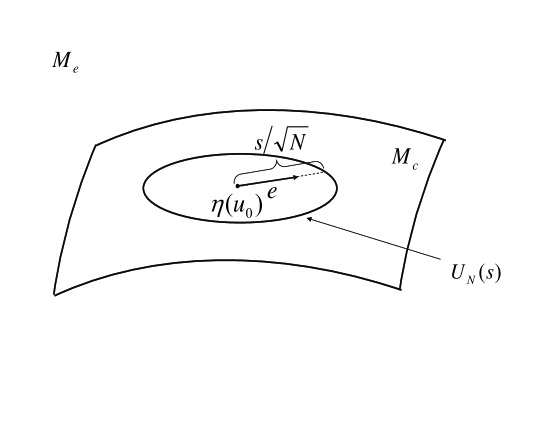
where [gab]delimited-[]subscript𝑔𝑎𝑏[g_{ab}] denotes the Riemannian metric on Mcsubscript𝑀𝑐M_{c} given by the Fisher information matrix, and e=(ea)𝑒superscript𝑒𝑎e=(e^{a}) denotes the m𝑚m-dimensional unit tangent vector of Mcsubscript𝑀𝑐M_{c} at u0subscript𝑢0u_{0}. The set UN(s)subscript𝑈𝑁𝑠U_{N}(s) consists of the points of Mcsubscript𝑀𝑐M_{c} which are separated from u0subscript𝑢0u_{0} by the geodesic distance s/N𝑠𝑁s/\sqrt{N} (Figure 1).

Refer to caption
Figure 1: The set of alternatives UN(s)subscript𝑈𝑁𝑠U_{N}(s) associated with an unbiased test of u=u0𝑢subscript𝑢0u=u_{0}.

We compare tests based on the average power P𝒯(s)subscript𝑃𝒯𝑠P_{\cal T}(s) defined by

P𝒯(s)=P𝒯(u)e=uUN(s)P𝒯(u)𝑑u/SN(s),subscript𝑃𝒯𝑠subscriptdelimited-⟨⟩subscript𝑃𝒯𝑢𝑒subscript𝑢subscript𝑈𝑁𝑠subscript𝑃𝒯𝑢differential-d𝑢subscript𝑆𝑁𝑠\displaystyle P_{{\cal T}}(s)=\langle P_{{\cal T}}(u)\rangle_{e}=\int_{u\in U_{N}(s)}P_{{\cal T}}(u)du/S_{N}(s),

where esubscript𝑒\langle\ \rangle_{e} means the average over all directions of e𝑒e, so that SN(s)subscript𝑆𝑁𝑠S_{N}(s) denotes the area of UN(s)subscript𝑈𝑁𝑠U_{N}(s).

Tests are required to satisfy the level and the unbiasedness conditions. We say a test 𝒯𝒯{\cal T} is of i𝑖i-th order level α𝛼\alpha, when

P𝒯(0)=α+O(Ni/2),subscript𝑃𝒯0𝛼𝑂superscript𝑁𝑖2\displaystyle P_{{\cal T}}(0)=\alpha+O(N^{-i/2}),

and we note that the unbiasedness condition

ddsP𝒯(s)|s=0=0evaluated-at𝑑𝑑𝑠subscript𝑃𝒯𝑠𝑠00\displaystyle\frac{d}{ds}P_{{\cal T}}(s)\Big{|}_{s=0}=0

is automatically satisfied, since the power P𝒯(s)subscript𝑃𝒯𝑠P_{{\cal T}}(s) is obtained by taking the average in all directions.

By expanding P𝒯(s)subscript𝑃𝒯𝑠P_{{\cal T}}(s) in the power series of N1/2superscript𝑁12N^{-1/2}, we have

P𝒯(s)=P𝒯1(s)+P𝒯2(s)N1/2+P𝒯3(s)N1+O(N3/2),subscript𝑃𝒯𝑠subscript𝑃𝒯1𝑠subscript𝑃𝒯2𝑠superscript𝑁12subscript𝑃𝒯3𝑠superscript𝑁1𝑂superscript𝑁32\displaystyle P_{{\cal T}}(s)=P_{{\cal T}1}(s)+P_{{\cal T}2}(s)N^{-1/2}+P_{{\cal T}3}(s)N^{-1}+O(N^{-3/2}),

and call P𝒯i(s)subscript𝑃𝒯𝑖𝑠P_{{\cal T}i}(s) the i𝑖i-th order power of a test 𝒯𝒯{\cal T} at s𝑠s. When discussing the i𝑖i-th order power, the tests are assumed to satisfy the level condition up to the same i𝑖i-th order.

A test 𝒯𝒯{\cal T} is said to be first-order uniformly efficient or said simply to be efficient in short when

P𝒯1(s)P𝒯1(s),s0,𝒯.formulae-sequencesubscript𝑃𝒯1𝑠subscript𝑃superscript𝒯1𝑠for-all𝑠0for-allsuperscript𝒯\displaystyle P_{{\cal T}1}(s)\geq P_{{\cal T}^{\prime}1}(s),\quad\forall s\geq 0,\quad\forall{\cal T}^{\prime}.

It can be shown that an efficient test is automatically second-order uniformly efficient, and that there does not in general exist a third-order uniformly efficient test. Thus we say that an efficient test 𝒯𝒯{\cal T} is third-order s0subscript𝑠0s_{0}-efficient when

P𝒯3(s0)P𝒯3(s0),efficient 𝒯.subscript𝑃𝒯3subscript𝑠0subscript𝑃superscript𝒯3subscript𝑠0for-allefficient 𝒯\displaystyle P_{{\cal T}3}(s_{0})\geq P_{{\cal T}^{\prime}3}(s_{0}),\quad\forall\textrm{efficient ${\cal T}^{\prime}$}.

In order to evaluate the power loss of a test, we next introduce the envelope power function by P(s)=sup𝒯P𝒯(s)superscript𝑃𝑠subscriptsupremum𝒯subscript𝑃𝒯𝑠P^{*}(s)=\sup_{{\cal T}}P_{{\cal T}}(s), where supsupremum\sup is taken at each s𝑠s separately. We expand it as

P(s)=P1(s)+P2(s)N1/2+P3(s)N1+O(N3/2),superscript𝑃𝑠superscriptsubscript𝑃1𝑠superscriptsubscript𝑃2𝑠superscript𝑁12superscriptsubscript𝑃3𝑠superscript𝑁1𝑂superscript𝑁32\displaystyle P^{*}(s)=P_{1}^{*}(s)+P_{2}^{*}(s)N^{-1/2}+P_{3}^{*}(s)N^{-1}+O(N^{-3/2}),

and call Pi(s)superscriptsubscript𝑃𝑖𝑠P_{i}^{*}(s) the i𝑖i-th order envelope power at s𝑠s. Then the (third-order) power-loss function ΔP𝒯(s)Δsubscript𝑃𝒯𝑠\Delta P_{{\cal T}}(s) of an efficient test 𝒯𝒯{\cal T} is defined by

ΔP𝒯(s)=P3(s)P𝒯3(s).Δsubscript𝑃𝒯𝑠superscriptsubscript𝑃3𝑠subscript𝑃𝒯3𝑠\displaystyle\Delta P_{{\cal T}}(s)=P_{3}^{*}(s)-P_{{\cal T}3}(s). (4.2)

4.3 Ancillary family associated with a test

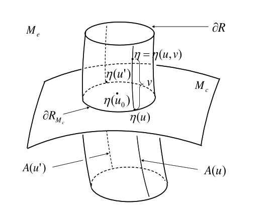
In calculating the power function P𝒯(s)subscript𝑃𝒯𝑠P_{{\cal T}}(s) of a test 𝒯𝒯{\cal T}, it is convenient to associate an ancillary family with a test. We attach to each point uMc𝑢subscript𝑀𝑐u\in M_{c} an (nm)𝑛𝑚(n-m)-dimensional smooth submanifold A(u)𝐴𝑢A(u) of Mesubscript𝑀𝑒M_{e} which transverses Mcsubscript𝑀𝑐M_{c} at θ(u)𝜃𝑢\theta(u) or equivalently at η(u)𝜂𝑢\eta(u). Such an A(u)𝐴𝑢A(u) is called an ancillary submanifold, and the union A={A(u)|uMc}𝐴conditional-set𝐴𝑢𝑢subscript𝑀𝑐A=\{A(u)\ |\ u\in M_{c}\} is called an ancillary family. Let RMc=RMcsubscript𝑅subscript𝑀𝑐𝑅subscript𝑀𝑐R_{M_{c}}=R\cap M_{c} be the intersection of Mcsubscript𝑀𝑐M_{c} and the critical region R𝑅R of a test 𝒯𝒯{\cal T}. An ancillary family A𝐴A is said to be associated with a test 𝒯𝒯{\cal T} when

R=uRMcA(u)={η|ηA(u),uRMc}.𝑅𝑢subscript𝑅subscript𝑀𝑐𝐴𝑢conditional-set𝜂formulae-sequence𝜂𝐴𝑢𝑢subscript𝑅subscript𝑀𝑐\displaystyle R=\underset{u\in R_{M_{c}}}{\cup}A(u)=\{\eta\ |\ \eta\in A(u),\ u\in R_{M_{c}}\}. (4.3)
Refer to caption
Figure 2: Ancillary family A={A(u)}𝐴𝐴𝑢A=\{A(u)\} and w=(u,v)𝑤𝑢𝑣w=(u,v)-coordinates associated with an unbiased test of u=u0𝑢subscript𝑢0u=u_{0}.

By introducing a coordinate system v=(vm+1,,vn)𝑣superscript𝑣𝑚1superscript𝑣𝑛v=(v^{m+1},\dots,v^{n}) to each A(u)𝐴𝑢A(u) such that the origin v=0𝑣0v=0 is at the intersection of A(u)𝐴𝑢A(u) and Mcsubscript𝑀𝑐M_{c}, we have a new local coordinate system of Mesubscript𝑀𝑒M_{e} (Figure 2)

w=(wα)=(ua,vκ),α=1,,n,a=1,,m,κ=m+1,,n,formulae-sequence𝑤superscript𝑤𝛼superscript𝑢𝑎superscript𝑣𝜅formulae-sequence𝛼1𝑛formulae-sequence𝑎1𝑚𝜅𝑚1𝑛\displaystyle w=(w^{\alpha})=(u^{a},v^{\kappa}),\quad\alpha=1,\dots,n,\quad a=1,\dots,m,\quad\kappa=m+1,\dots,n, (4.4)

and we use indices α,β,γ𝛼𝛽𝛾\alpha,\beta,\gamma and so on for quantities related to the coordinate system w𝑤w, and indices κ,λ,μ𝜅𝜆𝜇\kappa,\lambda,\mu and so on for quantities related to the coordinate system v𝑣v.

The critical region R𝑅R is written as

R={w=(u,v)|uRMc,vis arbitrary}𝑅conditional-set𝑤𝑢𝑣𝑢subscript𝑅subscript𝑀𝑐𝑣is arbitrary\displaystyle R=\{w=(u,v)\ |\ u\in R_{M_{c}},\ v\ \textrm{is arbitrary}\}

in the new coordinate system w𝑤w. The sufficient statistic x¯¯𝑥{\bar{x}} is transformed to w^=(u^,v^)^𝑤^𝑢^𝑣{\hat{w}}=({\hat{u}},{\hat{v}}) by x¯=η(w^)¯𝑥𝜂^𝑤{\bar{x}}=\eta({\hat{w}}), and the power P𝒯(u)subscript𝑃𝒯𝑢P_{{\cal T}}(u) is written as

P𝒯(u)=Rf(w^,u)𝑑w^=RMcA(u)f(w^,u)𝑑v^𝑑u^=RMcf(u^,u)𝑑u^,subscript𝑃𝒯𝑢subscript𝑅𝑓^𝑤𝑢differential-d^𝑤subscriptsubscript𝑅subscript𝑀𝑐subscript𝐴𝑢𝑓^𝑤𝑢differential-d^𝑣differential-d^𝑢subscriptsubscript𝑅subscript𝑀𝑐𝑓^𝑢𝑢differential-d^𝑢\displaystyle P_{{\cal T}}(u)=\int_{R}f({\hat{w}},u)d{\hat{w}}=\int_{R_{M_{c}}}\int_{A(u)}f({\hat{w}},u)d{\hat{v}}d{\hat{u}}=\int_{R_{M_{c}}}f({\hat{u}},u)d{\hat{u}},

where f(u^,u)=A(u)f(w^,u)𝑑v^𝑓^𝑢𝑢subscript𝐴𝑢𝑓^𝑤𝑢differential-d^𝑣f({\hat{u}},u)=\int_{A(u)}f({\hat{w}},u)d{\hat{v}} is the density function of u^^𝑢{\hat{u}} when the true parameter is u𝑢u.

4.4 Metric, connections and curvatures

The basic tensors of Mesubscript𝑀𝑒M_{e} are written as

gαβ(w)=BαiBβjgij(θ),Tαβγ(w)=BαiBβjBγkTijk(θ),Bαi=θiwα,formulae-sequencesubscript𝑔𝛼𝛽𝑤superscriptsubscript𝐵𝛼𝑖superscriptsubscript𝐵𝛽𝑗subscript𝑔𝑖𝑗𝜃formulae-sequencesubscript𝑇𝛼𝛽𝛾𝑤superscriptsubscript𝐵𝛼𝑖superscriptsubscript𝐵𝛽𝑗superscriptsubscript𝐵𝛾𝑘subscript𝑇𝑖𝑗𝑘𝜃superscriptsubscript𝐵𝛼𝑖superscript𝜃𝑖superscript𝑤𝛼\displaystyle g_{\alpha\beta}(w)=B_{\alpha}^{i}B_{\beta}^{j}g_{ij}(\theta),\quad T_{\alpha\beta\gamma}(w)=B_{\alpha}^{i}B_{\beta}^{j}B_{\gamma}^{k}T_{ijk}(\theta),\quad B_{\alpha}^{i}=\frac{\partial\theta^{i}}{\partial w^{\alpha}},

and the α𝛼\alpha-connection is given by

Γβγδ(α)(w)superscriptsubscriptΓ𝛽𝛾𝛿𝛼𝑤\displaystyle\Gamma_{\beta\gamma\delta}^{(\alpha)}(w) =BβiBγjBδkΓijk(α)(θ)+BδiβBγjgij(θ)=1α2Tβγδ+(βBγj)Bδjabsentsuperscriptsubscript𝐵𝛽𝑖superscriptsubscript𝐵𝛾𝑗superscriptsubscript𝐵𝛿𝑘superscriptsubscriptΓ𝑖𝑗𝑘𝛼𝜃superscriptsubscript𝐵𝛿𝑖subscript𝛽superscriptsubscript𝐵𝛾𝑗subscript𝑔𝑖𝑗𝜃1𝛼2subscript𝑇𝛽𝛾𝛿subscript𝛽superscriptsubscript𝐵𝛾𝑗subscript𝐵𝛿𝑗\displaystyle=B_{\beta}^{i}B_{\gamma}^{j}B_{\delta}^{k}\Gamma_{ijk}^{(\alpha)}(\theta)+B_{\delta}^{i}\partial_{\beta}B_{\gamma}^{j}g_{ij}(\theta)=\frac{1-\alpha}{2}T_{\beta\gamma\delta}+(\partial_{\beta}B_{\gamma}^{j})B_{\delta j}
=BβiBγjBδkΓ(α)ijk(η)+BδiβBγjgij(η)=1+α2Tβγδ+(βBγj)Bδj,absentsubscript𝐵𝛽𝑖subscript𝐵𝛾𝑗subscript𝐵𝛿𝑘superscriptΓ𝛼𝑖𝑗𝑘𝜂subscript𝐵𝛿𝑖subscript𝛽subscript𝐵𝛾𝑗superscript𝑔𝑖𝑗𝜂1𝛼2subscript𝑇𝛽𝛾𝛿subscript𝛽subscript𝐵𝛾𝑗superscriptsubscript𝐵𝛿𝑗\displaystyle=B_{\beta i}B_{\gamma j}B_{\delta k}\Gamma^{(\alpha)ijk}(\eta)+B_{\delta i}\partial_{\beta}B_{\gamma j}g^{ij}(\eta)=-\frac{1+\alpha}{2}T_{\beta\gamma\delta}+(\partial_{\beta}B_{\gamma j})B_{\delta}^{j},
Bβisubscript𝐵𝛽𝑖\displaystyle B_{\beta i} =ηiwβ=gijBβj,absentsubscript𝜂𝑖superscript𝑤𝛽subscript𝑔𝑖𝑗superscriptsubscript𝐵𝛽𝑗\displaystyle=\frac{\partial\eta_{i}}{\partial w^{\beta}}=g_{ij}B_{\beta}^{j},

in the w𝑤w-coordinate system. When we evaluate a quantity q(u,v)𝑞𝑢𝑣q(u,v) on Mcsubscript𝑀𝑐M_{c}, that is, at v=0𝑣0v=0, we often denote it by q(u)𝑞𝑢q(u) instead of by q(u,0)𝑞𝑢0q(u,0) for brevity’s sake. The metric tensors of Mcsubscript𝑀𝑐M_{c} and A(u)𝐴𝑢A(u) are given by

gab(u)=BaiBbjgij=BaiBbjgij,gκλ(u)=BκiBλjgij=BκiBλjgij,formulae-sequencesubscript𝑔𝑎𝑏𝑢superscriptsubscript𝐵𝑎𝑖superscriptsubscript𝐵𝑏𝑗subscript𝑔𝑖𝑗subscript𝐵𝑎𝑖subscript𝐵𝑏𝑗superscript𝑔𝑖𝑗subscript𝑔𝜅𝜆𝑢superscriptsubscript𝐵𝜅𝑖superscriptsubscript𝐵𝜆𝑗subscript𝑔𝑖𝑗subscript𝐵𝜅𝑖subscript𝐵𝜆𝑗superscript𝑔𝑖𝑗\displaystyle g_{ab}(u)=B_{a}^{i}B_{b}^{j}g_{ij}=B_{ai}B_{bj}g^{ij},\quad g_{\kappa\lambda}(u)=B_{\kappa}^{i}B_{\lambda}^{j}g_{ij}=B_{\kappa i}B_{\lambda j}g^{ij},

and then indices can be lowered or raised by using these metric tensors or their inverses gab(u),gκλ(u)superscript𝑔𝑎𝑏𝑢superscript𝑔𝜅𝜆𝑢g^{ab}(u),g^{\kappa\lambda}(u). The mixed part

gaκ(u)=BaiBκjgij=BaiBκjgijsubscript𝑔𝑎𝜅𝑢superscriptsubscript𝐵𝑎𝑖superscriptsubscript𝐵𝜅𝑗subscript𝑔𝑖𝑗subscript𝐵𝑎𝑖subscript𝐵𝜅𝑗superscript𝑔𝑖𝑗\displaystyle g_{a\kappa}(u)=B_{a}^{i}B_{\kappa}^{j}g_{ij}=B_{ai}B_{\kappa j}g^{ij}

is the inner product of the tangent vectors Basubscript𝐵𝑎B_{a} of Mcsubscript𝑀𝑐M_{c} and the tangent vectors Bκsubscript𝐵𝜅B_{\kappa} of A(u)𝐴𝑢A(u), which represents the angles between Mcsubscript𝑀𝑐M_{c} and A(u)𝐴𝑢A(u). When gaκ(u0)=0subscript𝑔𝑎𝜅subscript𝑢00g_{a\kappa}(u_{0})=0 holds at a point u0subscript𝑢0u_{0}, the ancillary family is said to be locally orthogonal at u0subscript𝑢0u_{0}. When gaκ(u)=0subscript𝑔𝑎𝜅𝑢0g_{a\kappa}(u)=0 holds at every u𝑢u, the ancillary family is said to be an orthogonal family.

For a locally orthogonal ancillary family, the inner product gaκ(us,e)subscript𝑔𝑎𝜅subscript𝑢𝑠𝑒g_{a\kappa}(u_{s,e}) at us,e=u0+se/Nsubscript𝑢𝑠𝑒subscript𝑢0𝑠𝑒𝑁u_{s,e}=u_{0}+se/\sqrt{N} is expanded as

gaκ(us,e)=Qbaκebs/N+O(N1),Qbaκ=bgaκ(u0),formulae-sequencesubscript𝑔𝑎𝜅subscript𝑢𝑠𝑒subscript𝑄𝑏𝑎𝜅superscript𝑒𝑏𝑠𝑁𝑂superscript𝑁1subscript𝑄𝑏𝑎𝜅subscript𝑏subscript𝑔𝑎𝜅subscript𝑢0\displaystyle g_{a\kappa}(u_{s,e})=Q_{ba\kappa}e^{b}s/\sqrt{N}+O(N^{-1}),\quad Q_{ba\kappa}=\partial_{b}g_{a\kappa}(u_{0}), (4.5)

where Qbaκsubscript𝑄𝑏𝑎𝜅Q_{ba\kappa} is the tensor quantity characterizing the angles between us,eUN(s)A(us,e)subscriptsubscript𝑢𝑠𝑒subscript𝑈𝑁𝑠𝐴subscript𝑢𝑠𝑒\cup_{u_{s,e}\in U_{N}(s)}A(u_{s,e}) and Mcsubscript𝑀𝑐M_{c}.

When the ancillary family is locally orthogonal, the mixed parts Γabκ(1)(u0)superscriptsubscriptΓ𝑎𝑏𝜅1subscript𝑢0\Gamma_{ab\kappa}^{(1)}(u_{0}) and Γκλa(1)(u0)superscriptsubscriptΓ𝜅𝜆𝑎1subscript𝑢0\Gamma_{\kappa\lambda a}^{(-1)}(u_{0}) of the ±1plus-or-minus1\pm 1-connections are tensor quantities, which are denoted by

Habκ(1)(u0)=Γabκ(1)(u0)=(aBbi)Bκi,Hκλa(1)(u0)=Γκλa(1)(u0)=(κBλi)Bai.formulae-sequencesuperscriptsubscript𝐻𝑎𝑏𝜅1subscript𝑢0superscriptsubscriptΓ𝑎𝑏𝜅1subscript𝑢0subscript𝑎superscriptsubscript𝐵𝑏𝑖subscript𝐵𝜅𝑖superscriptsubscript𝐻𝜅𝜆𝑎1subscript𝑢0superscriptsubscriptΓ𝜅𝜆𝑎1subscript𝑢0subscript𝜅subscript𝐵𝜆𝑖superscriptsubscript𝐵𝑎𝑖\displaystyle H_{ab\kappa}^{(1)}(u_{0})=\Gamma_{ab\kappa}^{(1)}(u_{0})=(\partial_{a}B_{b}^{i})B_{\kappa i},\quad H_{\kappa\lambda a}^{(-1)}(u_{0})=\Gamma_{\kappa\lambda a}^{(-1)}(u_{0})=(\partial_{\kappa}B_{\lambda i})B_{a}^{i}. (4.6)

These tensor quantities Habκ(1)(u0)superscriptsubscript𝐻𝑎𝑏𝜅1subscript𝑢0H_{ab\kappa}^{(1)}(u_{0}) and Hκλa(1)(u0)superscriptsubscript𝐻𝜅𝜆𝑎1subscript𝑢0H_{\kappa\lambda a}^{(-1)}(u_{0}) are called the ±1plus-or-minus1\pm 1-ES curvature tensors of Mcsubscript𝑀𝑐M_{c} and A(u0)𝐴subscript𝑢0A(u_{0}) in Mesubscript𝑀𝑒M_{e}, respectively. When Hκλa(1)(u0)=0superscriptsubscript𝐻𝜅𝜆𝑎1subscript𝑢00H_{\kappa\lambda a}^{(-1)}(u_{0})=0 holds, the ancillary family A𝐴A is said to be mixture flat (m𝑚m-flat) at u0subscript𝑢0u_{0} in Mesubscript𝑀𝑒M_{e}.

Related to the 111-ES curvature tensor Habκ(1)superscriptsubscript𝐻𝑎𝑏𝜅1H_{ab\kappa}^{(1)} of Mcsubscript𝑀𝑐M_{c} in Mesubscript𝑀𝑒M_{e}, we also define

Hκ(1)=1mHabκ(1)gab,Kabκ(1)=Habκ(1)gabHκ(1).formulae-sequencesuperscriptsubscript𝐻𝜅11𝑚superscriptsubscript𝐻𝑎𝑏𝜅1superscript𝑔𝑎𝑏superscriptsubscript𝐾𝑎𝑏𝜅1superscriptsubscript𝐻𝑎𝑏𝜅1subscript𝑔𝑎𝑏superscriptsubscript𝐻𝜅1\displaystyle H_{\kappa}^{(1)}=\frac{1}{m}H_{ab\kappa}^{(1)}g^{ab},\quad K_{ab\kappa}^{(1)}=H_{ab\kappa}^{(1)}-g_{ab}H_{\kappa}^{(1)}. (4.7)

The first Hκ(1)superscriptsubscript𝐻𝜅1H_{\kappa}^{(1)} is called the mean 111-ES curvature tensor of Mcsubscript𝑀𝑐M_{c} in Mesubscript𝑀𝑒M_{e}, and the second Kabκ(1)superscriptsubscript𝐾𝑎𝑏𝜅1K_{ab\kappa}^{(1)} is called the 111-ES umbilic tensor of Mcsubscript𝑀𝑐M_{c} in Mesubscript𝑀𝑒M_{e}, respectively. When Kabκ(1)0superscriptsubscript𝐾𝑎𝑏𝜅10K_{ab\kappa}^{(1)}\equiv 0 holds, Mcsubscript𝑀𝑐M_{c} is said to be totally exponential umbilic (e𝑒e-umbilic) in Mesubscript𝑀𝑒M_{e}.

We remark that the 1-ES curvature tensor variable hab(1)(x,u)superscriptsubscript𝑎𝑏1𝑥𝑢h_{ab}^{(1)}(x,u) of Mcsubscript𝑀𝑐M_{c} in Mcsubscriptsubscript𝑀𝑐{\cal R}_{M_{c}} can be also introduced and expressed as

hab(1)(x,u)superscriptsubscript𝑎𝑏1𝑥𝑢\displaystyle h_{ab}^{(1)}(x,u) =abl1(x,u)+gab(u)Γab(1)c(u)cl1(x,u)absentsubscript𝑎subscript𝑏subscript𝑙1𝑥𝑢subscript𝑔𝑎𝑏𝑢superscriptsubscriptΓ𝑎𝑏1𝑐𝑢subscript𝑐subscript𝑙1𝑥𝑢\displaystyle=\partial_{a}\partial_{b}l_{1}(x,u)+g_{ab}(u)-\Gamma_{ab}^{(1)c}(u)\partial_{c}l_{1}(x,u)
=Habκ(1)(u)gκλ(u)λl1(x,u),l1(x,u)=logfc(x,u).formulae-sequenceabsentsuperscriptsubscript𝐻𝑎𝑏𝜅1𝑢superscript𝑔𝜅𝜆𝑢subscript𝜆subscript𝑙1𝑥𝑢subscript𝑙1𝑥𝑢subscript𝑓𝑐𝑥𝑢\displaystyle=H_{ab\kappa}^{(1)}(u)g^{\kappa\lambda}(u)\partial_{\lambda}l_{1}(x,u),\quad l_{1}(x,u)=\log f_{c}(x,u). (4.8)

This expression shows that the 1-ES curvature tensor Habκ(1)(u)superscriptsubscript𝐻𝑎𝑏𝜅1𝑢H_{ab\kappa}^{(1)}(u) of Mcsubscript𝑀𝑐M_{c} in Mesubscript𝑀𝑒M_{e} and the 1-ES curvature tensor variable hab(1)(x,u)superscriptsubscript𝑎𝑏1𝑥𝑢h_{ab}^{(1)}(x,u) of Mcsubscript𝑀𝑐M_{c} in Mcsubscriptsubscript𝑀𝑐{\cal R}_{M_{c}} are the equivalent notions. Hence when Kabκ(1)0superscriptsubscript𝐾𝑎𝑏𝜅10K_{ab\kappa}^{(1)}\equiv 0 holds, Mcsubscript𝑀𝑐M_{c} can also said to be totally e𝑒e-umbilic in RMcsubscript𝑅subscript𝑀𝑐R_{M_{c}}.

4.5 First-order power

The first-order analysis is based on the normal distribution on f(w^,u)𝑓^𝑤𝑢f({\hat{w}},u), and we have the following result (cf. Amari, 1985, Theorem 6.17).

Proposition 4.1.

A test 𝒯𝒯{\cal T} is first-order uniformly efficient, if and only if the associated ancillary family is asymptotically orthogonal in the sense

gaκ(u)=O(N1/2),uRMc=RMc,formulae-sequencesubscript𝑔𝑎𝜅𝑢𝑂superscript𝑁12for-all𝑢subscript𝑅subscript𝑀𝑐𝑅subscript𝑀𝑐\displaystyle g_{a\kappa}(u)=O(N^{-1/2}),\quad\forall u\in\partial R_{M_{c}}=\partial R\cap M_{c},

and the optimal intersection RMc=RMcsuperscriptsubscript𝑅subscript𝑀𝑐superscript𝑅subscript𝑀𝑐R_{M_{c}}^{*}=R^{*}\cap M_{c} is given by

RMc={u~0|gab(u0)u~0au~0bc02},u~0=N(u^u0),c02=χm,α2,formulae-sequencesuperscriptsubscript𝑅subscript𝑀𝑐conditional-setsubscript~𝑢0subscript𝑔𝑎𝑏subscript𝑢0superscriptsubscript~𝑢0𝑎superscriptsubscript~𝑢0𝑏superscriptsubscript𝑐02formulae-sequencesubscript~𝑢0𝑁^𝑢subscript𝑢0superscriptsubscript𝑐02superscriptsubscript𝜒𝑚𝛼2\displaystyle R_{M_{c}}^{*}=\{{\tilde{u}}_{0}\ |\ g_{ab}(u_{0}){\tilde{u}}_{0}^{a}{\tilde{u}}_{0}^{b}\geq c_{0}^{2}\},\quad{\tilde{u}}_{0}=\sqrt{N}({\hat{u}}-u_{0}),\quad c_{0}^{2}=\chi_{m,\alpha}^{2},

where χm,α2superscriptsubscript𝜒𝑚𝛼2\chi_{m,\alpha}^{2} denotes the upper 100α%100percent𝛼100\alpha\% point of the χ2superscript𝜒2\chi^{2}-distribution with m𝑚m degrees of freedom. The first-order envelope power function P1(s)superscriptsubscript𝑃1𝑠P_{1}^{*}(s) is expressed as

P1(s)=10c0Zm(0)(s,r)𝑑r,superscriptsubscript𝑃1𝑠1superscriptsubscript0subscript𝑐0superscriptsubscript𝑍𝑚0𝑠𝑟differential-d𝑟\displaystyle P_{1}^{*}(s)=1-\int_{0}^{c_{0}}Z_{m}^{(0)}(s,r)dr,
Zm(0)(s,r)=(2π)m/2rm1Sm2exp{12(s2+r2)}Ak(0)(s,r),superscriptsubscript𝑍𝑚0𝑠𝑟superscript2𝜋𝑚2superscript𝑟𝑚1subscript𝑆𝑚212superscript𝑠2superscript𝑟2superscriptsubscript𝐴𝑘0𝑠𝑟\displaystyle Z_{m}^{(0)}(s,r)=(2\pi)^{-m/2}r^{m-1}S_{m-2}\exp\bigg{\{}-\frac{1}{2}(s^{2}+r^{2})\bigg{\}}A_{k}^{(0)}(s,r),
Ak(0)(s,r)=0πsinm2φexp(srcosφ)dφ,superscriptsubscript𝐴𝑘0𝑠𝑟superscriptsubscript0𝜋superscript𝑚2𝜑𝑠𝑟𝜑𝑑𝜑\displaystyle A_{k}^{(0)}(s,r)=\int_{0}^{\pi}\sin^{m-2}\varphi\exp(sr\cos\varphi)d\varphi,

where Sm2subscript𝑆𝑚2S_{m-2} denotes the area of the (m2)𝑚2(m-2)-dimensional unit sphere with S0=2subscript𝑆02S_{0}=2. Note that Zm(0)(s,r)superscriptsubscript𝑍𝑚0𝑠𝑟Z_{m}^{(0)}(s,r) is the density function of the χ2superscript𝜒2\chi^{2}-distribution with m𝑚m degrees of freedom and non-centrality parameter s2superscript𝑠2s^{2}.

4.6 Second- and third-order powers

These powers can be calculated by taking account of the higher-order terms of f(w^,u)𝑓^𝑤𝑢f({\hat{w}},u), and by assuming the intersection RMcsubscript𝑅subscript𝑀𝑐R_{M_{c}} as

RMc={u~0|gab(u0)u~0au~0b(c0+ϵ)2},u~0a=u~0a+Γβγ(1)agβγ(u^)/(2N),formulae-sequencesubscript𝑅subscript𝑀𝑐conditional-setsubscript~𝑢0subscript𝑔𝑎𝑏subscript𝑢0superscriptsubscript~𝑢0absent𝑎superscriptsubscript~𝑢0absent𝑏superscriptsubscript𝑐0italic-ϵ2superscriptsubscript~𝑢0absent𝑎superscriptsubscript~𝑢0𝑎superscriptsubscriptΓ𝛽𝛾1𝑎superscript𝑔𝛽𝛾^𝑢2𝑁\displaystyle R_{M_{c}}=\{{\tilde{u}}_{0}\ |\ g_{ab}(u_{0}){\tilde{u}}_{0}^{*a}{\tilde{u}}_{0}^{*b}\geq(c_{0}+\epsilon)^{2}\},\quad{\tilde{u}}_{0}^{*a}={\tilde{u}}_{0}^{a}+\Gamma_{\beta\gamma}^{(-1)a}g^{\beta\gamma}({\hat{u}})/(2\sqrt{N}), (4.9)

where u~0superscriptsubscript~𝑢0{\tilde{u}}_{0}^{*} is the bias-corrected version of u~0subscript~𝑢0{\tilde{u}}_{0}, and ϵitalic-ϵ\epsilon is introduced to adjust to the level condition up to O(N1)𝑂superscript𝑁1O(N^{-1}). It is shown that ϵ=O(N1)italic-ϵ𝑂superscript𝑁1\epsilon=O(N^{-1}), which depends on the ancillary family through Hκλa(1)superscriptsubscript𝐻𝜅𝜆𝑎1H_{\kappa\lambda a}^{(-1)} and Qabκsubscript𝑄𝑎𝑏𝜅Q_{ab\kappa}. Hence it follows that the second-order power function P𝒯2(s)subscript𝑃𝒯2𝑠P_{{\cal T}2}(s) is common to all the first-order efficient tests (see Appendices 1, 2).

Here we introduce a class of efficient tests whose ancillary family satisfies

Q(ab)κ=k1Kabκ(1)+k2gabHκ(1),Q(ab)κ=12(Qabκ+Qbaκ),k1,k2,formulae-sequencesubscript𝑄𝑎𝑏𝜅subscript𝑘1superscriptsubscript𝐾𝑎𝑏𝜅1subscript𝑘2subscript𝑔𝑎𝑏superscriptsubscript𝐻𝜅1formulae-sequencesubscript𝑄𝑎𝑏𝜅12subscript𝑄𝑎𝑏𝜅subscript𝑄𝑏𝑎𝜅subscript𝑘1subscript𝑘2\displaystyle Q_{(ab)\kappa}=k_{1}K_{ab\kappa}^{(1)}+k_{2}g_{ab}H_{\kappa}^{(1)},\quad Q_{(ab)\kappa}=\frac{1}{2}(Q_{ab\kappa}+Q_{ba\kappa}),\quad k_{1},k_{2}\in{\mathbb{R}}, (4.10)

and a test 𝒯𝒯{\cal T} with a pair of proportions (k1,k2)subscript𝑘1subscript𝑘2(k_{1},k_{2}) is said to be the k=(k1,k2)𝑘subscript𝑘1subscript𝑘2k=(k_{1},k_{2})-test. Then after cumbersome calculations, we have the following result on the third-order efficiency of a k=(k1,k2)𝑘subscript𝑘1subscript𝑘2k=(k_{1},k_{2})-test, which is the correction of Theorem 6.18 in Amari (1985).

Proposition 4.2.

The third-order power loss function ΔP𝒦(s)Δsubscript𝑃𝒦𝑠\Delta P_{\cal K}(s) of a k=(k1,k2)𝑘subscript𝑘1subscript𝑘2k=(k_{1},k_{2})-test 𝒯𝒯{\cal T} is given by

ΔP𝒦(s)Δsubscript𝑃𝒦𝑠\displaystyle\Delta P_{\cal K}(s) =κ2ΔP1(s)+γ2ΔP2(s)+HA(1)2ξ0m(s),absentsuperscript𝜅2Δsubscript𝑃1𝑠superscript𝛾2Δsubscript𝑃2𝑠superscriptsubscript𝐻𝐴12subscript𝜉0𝑚𝑠\displaystyle=\kappa^{2}\Delta P_{1}(s)+\gamma^{2}\Delta P_{2}(s)+H_{A}^{(-1)2}\xi_{0m}(s), (4.11)

where

ΔP1(s)=ξ1m(s){K1K1m(s)}2,ΔP2(s)=ξ2m(s){K2K2m(s)}2,formulae-sequenceΔsubscript𝑃1𝑠subscript𝜉1𝑚𝑠superscriptsubscript𝐾1subscript𝐾1𝑚𝑠2Δsubscript𝑃2𝑠subscript𝜉2𝑚𝑠superscriptsubscript𝐾2subscript𝐾2𝑚𝑠2\displaystyle\Delta P_{1}(s)=\xi_{1m}(s)\{K_{1}-K_{1m}(s)\}^{2},\quad\Delta P_{2}(s)=\xi_{2m}(s)\{K_{2}-K_{2m}(s)\}^{2}, (4.12)
κ2=Kabκ(1)Kcdλ(1)gacgbdgκλ,γ2=mHκ(1)Hλ(1)gκλ,formulae-sequencesuperscript𝜅2superscriptsubscript𝐾𝑎𝑏𝜅1superscriptsubscript𝐾𝑐𝑑𝜆1superscript𝑔𝑎𝑐superscript𝑔𝑏𝑑superscript𝑔𝜅𝜆superscript𝛾2𝑚superscriptsubscript𝐻𝜅1superscriptsubscript𝐻𝜆1superscript𝑔𝜅𝜆\displaystyle\kappa^{2}=K_{ab\kappa}^{(1)}K_{cd\lambda}^{(1)}g^{ac}g^{bd}g^{\kappa\lambda},\quad\gamma^{2}=mH_{\kappa}^{(1)}H_{\lambda}^{(1)}g^{\kappa\lambda},
HA(1)2=Hκλa(1)Hμνb(1)gκμgλνgab.superscriptsubscript𝐻𝐴12superscriptsubscript𝐻𝜅𝜆𝑎1superscriptsubscript𝐻𝜇𝜈𝑏1superscript𝑔𝜅𝜇superscript𝑔𝜆𝜈superscript𝑔𝑎𝑏\displaystyle H_{A}^{(-1)2}=H_{\kappa\lambda a}^{(-1)}H_{\mu\nu b}^{(-1)}g^{\kappa\mu}g^{\lambda\nu}g^{ab}.

An efficient k=(k1,k2)𝑘subscript𝑘1subscript𝑘2k=(k_{1},k_{2})-test 𝒯𝒯{\cal T} is third-order s0subscript𝑠0s_{0}-efficient if and only if

k1=K1m(s0),k2=K2m(s0),Hκλa(1)(u0)=0.formulae-sequencesubscript𝑘1subscript𝐾1𝑚subscript𝑠0formulae-sequencesubscript𝑘2subscript𝐾2𝑚subscript𝑠0superscriptsubscript𝐻𝜅𝜆𝑎1subscript𝑢00\displaystyle k_{1}=K_{1m}(s_{0}),\quad k_{2}=K_{2m}(s_{0}),\quad H_{\kappa\lambda a}^{(-1)}(u_{0})=0. (4.13)

In the above expressions,

K1m(s0)=J1m(s0),K2m(s0)=J2m(s0)+ξ1m(s0){J1m(s0)J2m(s0)}ξ2m(s0),formulae-sequencesubscript𝐾1𝑚subscript𝑠0subscript𝐽1𝑚subscript𝑠0subscript𝐾2𝑚subscript𝑠0subscript𝐽2𝑚subscript𝑠0subscript𝜉1𝑚subscript𝑠0subscript𝐽1𝑚subscript𝑠0subscript𝐽2𝑚subscript𝑠0subscript𝜉2𝑚subscript𝑠0\displaystyle K_{1m}(s_{0})=J_{1m}(s_{0}),\quad K_{2m}(s_{0})=J_{2m}(s_{0})+\frac{\xi_{1m}(s_{0})\{J_{1m}(s_{0})-J_{2m}(s_{0})\}}{\xi_{2m}(s_{0})}, (4.14)

and

ξ1m(s)=12m(m+2)[2c02sZm(1)(s,c0)2c0s2{Zm(0)(s,c0)Zm(2)(s,c0)}+0c0f1m(s,r)𝑑r],subscript𝜉1𝑚𝑠12𝑚𝑚2delimited-[]2superscriptsubscript𝑐02𝑠superscriptsubscript𝑍𝑚1𝑠subscript𝑐02subscript𝑐0superscript𝑠2superscriptsubscript𝑍𝑚0𝑠subscript𝑐0superscriptsubscript𝑍𝑚2𝑠subscript𝑐0superscriptsubscript0subscript𝑐0subscript𝑓1𝑚𝑠𝑟differential-d𝑟\displaystyle\xi_{1m}(s)=\frac{1}{2m(m+2)}\left[2c_{0}^{2}sZ_{m}^{(1)}(s,c_{0})-2c_{0}s^{2}\{Z_{m}^{(0)}(s,c_{0})-Z_{m}^{(2)}(s,c_{0})\}+\int_{0}^{c_{0}}f_{1m}(s,r)dr\right],
f1m(s,r)=msrZm(1)(s,r)+s2{(m+2)Zm(0)(s,r)2kZk(2)(s,r)}+2s3r{Zk(1)(s,r)Zm(3)(s,r)},subscript𝑓1𝑚𝑠𝑟𝑚𝑠𝑟superscriptsubscript𝑍𝑚1𝑠𝑟superscript𝑠2𝑚2superscriptsubscript𝑍𝑚0𝑠𝑟2𝑘superscriptsubscript𝑍𝑘2𝑠𝑟2superscript𝑠3𝑟superscriptsubscript𝑍𝑘1𝑠𝑟superscriptsubscript𝑍𝑚3𝑠𝑟\displaystyle f_{1m}(s,r)=-msrZ_{m}^{(1)}(s,r)+s^{2}\{(m+2)Z_{m}^{(0)}(s,r)-2kZ_{k}^{(2)}(s,r)\}+2s^{3}r\{Z_{k}^{(1)}(s,r)-Z_{m}^{(3)}(s,r)\},
ξ2m(s)=12m(m+2)[c02sZm(1)(s,c0)+c0s2{Zm(0)(s,c0)Zm(2)(s,c0)}+0c0f2m(s,r)𝑑r],superscriptsubscript𝜉2𝑚𝑠12𝑚𝑚2delimited-[]superscriptsubscript𝑐02𝑠superscriptsubscript𝑍𝑚1𝑠subscript𝑐0subscript𝑐0superscript𝑠2superscriptsubscript𝑍𝑚0𝑠subscript𝑐0superscriptsubscript𝑍𝑚2𝑠subscript𝑐0superscriptsubscript0subscript𝑐0subscript𝑓2𝑚𝑠𝑟differential-d𝑟\displaystyle\xi_{2m}^{\prime}(s)=\frac{1}{2m(m+2)}\left[c_{0}^{2}sZ_{m}^{(1)}(s,c_{0})+c_{0}s^{2}\{Z_{m}^{(0)}(s,c_{0})-Z_{m}^{(2)}(s,c_{0})\}+\int_{0}^{c_{0}}f_{2m}(s,r)dr\right],
f2m(s,r)=srZm(1)(s,r)s2{2Zm(0)(s,r)mZm(2)(s,r)}s3r{Zm(1)(s,r)Zm(3)(s,r)},subscript𝑓2𝑚𝑠𝑟𝑠𝑟superscriptsubscript𝑍𝑚1𝑠𝑟superscript𝑠22superscriptsubscript𝑍𝑚0𝑠𝑟𝑚superscriptsubscript𝑍𝑚2𝑠𝑟superscript𝑠3𝑟superscriptsubscript𝑍𝑚1𝑠𝑟superscriptsubscript𝑍𝑚3𝑠𝑟\displaystyle f_{2m}(s,r)=srZ_{m}^{(1)}(s,r)-s^{2}\{2Z_{m}^{(0)}(s,r)-mZ_{m}^{(2)}(s,r)\}-s^{3}r\{Z_{m}^{(1)}(s,r)-Z_{m}^{(3)}(s,r)\},
J1m(s)=ξ3m(s)2ξ1m(s),J2m(s)=ξ4m(s)2ξ2m(s),ξ2m(s)=ξ1m(s)+mξ2m(s),formulae-sequencesubscript𝐽1𝑚𝑠subscript𝜉3𝑚𝑠2subscript𝜉1𝑚𝑠formulae-sequencesubscript𝐽2𝑚𝑠subscript𝜉4𝑚𝑠2superscriptsubscript𝜉2𝑚𝑠subscript𝜉2𝑚𝑠subscript𝜉1𝑚𝑠𝑚superscriptsubscript𝜉2𝑚𝑠\displaystyle J_{1m}(s)=\frac{\xi_{3m}(s)}{2\xi_{1m}(s)},\quad J_{2m}(s)=\frac{\xi_{4m}(s)}{2\xi_{2m}^{\prime}(s)},\quad\xi_{2m}(s)=\xi_{1m}(s)+m\xi_{2m}^{\prime}(s),
ξ3m(s)=12m(m+2)[4c02sZm(1)(s,c0)2c0s2Zm(0)(s,c0)+0c0f3m(s,r)𝑑r],subscript𝜉3𝑚𝑠12𝑚𝑚2delimited-[]4superscriptsubscript𝑐02𝑠superscriptsubscript𝑍𝑚1𝑠subscript𝑐02subscript𝑐0superscript𝑠2superscriptsubscript𝑍𝑚0𝑠subscript𝑐0superscriptsubscript0subscript𝑐0subscript𝑓3𝑚𝑠𝑟differential-d𝑟\displaystyle\xi_{3m}(s)=\frac{1}{2m(m+2)}\left[4c_{0}^{2}sZ_{m}^{(1)}(s,c_{0})-2c_{0}s^{2}Z_{m}^{(0)}(s,c_{0})+\int_{0}^{c_{0}}f_{3m}(s,r)dr\right],
f3m(s,r)=2msrZm(1)(s,r)+2ms2Zm(0)(s,r),subscript𝑓3𝑚𝑠𝑟2𝑚𝑠𝑟superscriptsubscript𝑍𝑚1𝑠𝑟2𝑚superscript𝑠2superscriptsubscript𝑍𝑚0𝑠𝑟\displaystyle f_{3m}(s,r)=-2msrZ_{m}^{(1)}(s,r)+2ms^{2}Z_{m}^{(0)}(s,r),
ξ4m(s)=12m(m+2)[2c02sZm(1)(s,c0)c0s2Zm(0)(s,c0)+0c0f4m(s,r)𝑑r],subscript𝜉4𝑚𝑠12𝑚𝑚2delimited-[]2superscriptsubscript𝑐02𝑠superscriptsubscript𝑍𝑚1𝑠subscript𝑐0subscript𝑐0superscript𝑠2superscriptsubscript𝑍𝑚0𝑠subscript𝑐0superscriptsubscript0subscript𝑐0subscript𝑓4𝑚𝑠𝑟differential-d𝑟\displaystyle\xi_{4m}(s)=\frac{1}{2m(m+2)}\left[2c_{0}^{2}sZ_{m}^{(1)}(s,c_{0})-c_{0}s^{2}Z_{m}^{(0)}(s,c_{0})+\int_{0}^{c_{0}}f_{4m}(s,r)dr\right],
f4m(s,r)=2srZm(1)(s,r)2s2Zm(0)(s,r),subscript𝑓4𝑚𝑠𝑟2𝑠𝑟superscriptsubscript𝑍𝑚1𝑠𝑟2superscript𝑠2superscriptsubscript𝑍𝑚0𝑠𝑟\displaystyle f_{4m}(s,r)=2srZ_{m}^{(1)}(s,r)-2s^{2}Z_{m}^{(0)}(s,r),
ξ0m(s)=14m0c0f0m(s,r)𝑑r,subscript𝜉0𝑚𝑠14𝑚superscriptsubscript0subscript𝑐0subscript𝑓0𝑚𝑠𝑟differential-d𝑟\displaystyle\xi_{0m}(s)=\frac{1}{4m}\int_{0}^{c_{0}}f_{0m}(s,r)dr,
f0m(s,r)=srZm(1)(s,r)+s2Zm(0)(s,r),subscript𝑓0𝑚𝑠𝑟𝑠𝑟superscriptsubscript𝑍𝑚1𝑠𝑟superscript𝑠2superscriptsubscript𝑍𝑚0𝑠𝑟\displaystyle f_{0m}(s,r)=-srZ_{m}^{(1)}(s,r)+s^{2}Z_{m}^{(0)}(s,r),
Zm(l)(s,r)=(2π)m/2rm1Sm2exp{12(s2+r2)}Am(l)(s,r),superscriptsubscript𝑍𝑚𝑙𝑠𝑟superscript2𝜋𝑚2superscript𝑟𝑚1subscript𝑆𝑚212superscript𝑠2superscript𝑟2superscriptsubscript𝐴𝑚𝑙𝑠𝑟\displaystyle Z_{m}^{(l)}(s,r)=(2\pi)^{-m/2}r^{m-1}S_{m-2}\exp\left\{-\frac{1}{2}(s^{2}+r^{2})\right\}A_{m}^{(l)}(s,r),
Am(l)(s,r)=0πsinm2φcoslφexp(srcosφ)dφ.superscriptsubscript𝐴𝑚𝑙𝑠𝑟superscriptsubscript0𝜋superscript𝑚2𝜑superscript𝑙𝜑𝑠𝑟𝜑𝑑𝜑\displaystyle A_{m}^{(l)}(s,r)=\int_{0}^{\pi}\sin^{m-2}\varphi\cos^{l}\varphi\exp(sr\cos\varphi)d\varphi.
Refer to caption
Figure 3: Power loss coefficient ξ0m(s)subscript𝜉0𝑚𝑠\xi_{0m}(s).
Refer to caption
Figure 4: Power loss coefficient ξ1m(s)subscript𝜉1𝑚𝑠\xi_{1m}(s).
Refer to caption
Figure 5: Power loss coefficient ξ2m(s)subscript𝜉2𝑚𝑠\xi_{2m}(s).
Refer to caption
Figure 6: Optimal proportion K1m(s)subscript𝐾1𝑚𝑠K_{1m}(s).
Refer to caption
Figure 7: Optimal proportion K2m(s)subscript𝐾2𝑚𝑠K_{2m}(s).

The third-order power loss function P𝒦(s)subscript𝑃𝒦𝑠P_{\cal K}(s) of a k𝑘k-test given by (4.11) depends on three kinds of nonnegative scalar curvatures κ2,γ2superscript𝜅2superscript𝛾2\kappa^{2},\gamma^{2} and HA(1)2superscriptsubscript𝐻𝐴12H_{A}^{(-1)2}. Among them, κ2superscript𝜅2\kappa^{2} measures the square of the anisotropy of the 111-ES curvature of Mcsubscript𝑀𝑐M_{c} in Mesubscript𝑀𝑒M_{e}, and γ2superscript𝛾2\gamma^{2} measures the square of the mean 111-ES curvature of Mcsubscript𝑀𝑐M_{c} in Mesubscript𝑀𝑒M_{e}. On the other hand, HA(1)2superscriptsubscript𝐻𝐴12H_{A}^{(-1)2} measures the square of the (1)1(-1)-ES curvature of the ancillary subspace A(u0)𝐴subscript𝑢0A(u_{0}) in Mesubscript𝑀𝑒M_{e} associated with a k𝑘k-test.

Figures 3, 4, 5 show the power loss coefficients ξ0m(s),ξ1m(s),ξ2m(s)subscript𝜉0𝑚𝑠subscript𝜉1𝑚𝑠subscript𝜉2𝑚𝑠\xi_{0m}(s),\ \xi_{1m}(s),\ \xi_{2m}(s) given in (4.11), (4.12) as functions of s𝑠s in the cases of m=2,3,4,5𝑚2345m=2,3,4,5 with α=0.05𝛼0.05\alpha=0.05.

Figures 6, 7 show the optimal proportions K1m(s),K2m(s)subscript𝐾1𝑚𝑠subscript𝐾2𝑚𝑠K_{1m}(s),\ K_{2m}(s) given by (4.14) as functions of s𝑠s in the cases of m=2,3,4,5𝑚2345m=2,3,4,5 with α=0.05𝛼0.05\alpha=0.05.

Widely used typical tests can be regarded as the m𝑚m-flat k𝑘k-tests in the following manner (cf. Amari, 1985, Chapter 6). The m.l.e. test (MLT)𝑀𝐿𝑇(MLT) or the Wald test uses

gab(u^mle)(u^mleau0a)(u^mlebu0b)orgab(u0)(u^mleau0a)(u^mlebu0b)subscript𝑔𝑎𝑏subscript^𝑢𝑚𝑙𝑒superscriptsubscript^𝑢𝑚𝑙𝑒𝑎superscriptsubscript𝑢0𝑎superscriptsubscript^𝑢𝑚𝑙𝑒𝑏superscriptsubscript𝑢0𝑏orsubscript𝑔𝑎𝑏subscript𝑢0superscriptsubscript^𝑢𝑚𝑙𝑒𝑎superscriptsubscript𝑢0𝑎superscriptsubscript^𝑢𝑚𝑙𝑒𝑏superscriptsubscript𝑢0𝑏\displaystyle g_{ab}(\hat{u}_{mle})(\hat{u}_{mle}^{a}-u_{0}^{a})(\hat{u}_{mle}^{b}-u_{0}^{b})\quad\textrm{or}\quad g_{ab}(u_{0})(\hat{u}_{mle}^{a}-u_{0}^{a})(\hat{u}_{mle}^{b}-u_{0}^{b})

as the test statistic, where u^mlesubscript^𝑢𝑚𝑙𝑒\hat{u}_{mle} denotes the maximum likelihood estimator of u𝑢u, and its characteristic is

k1=k2=0,Hκλa(1)(u)0.formulae-sequencesubscript𝑘1subscript𝑘20superscriptsubscript𝐻𝜅𝜆𝑎1𝑢0\displaystyle k_{1}=k_{2}=0,\quad H_{\kappa\lambda a}^{(-1)}(u)\equiv 0. (4.15)

The likelihood ratio test (LRT)𝐿𝑅𝑇(LRT) uses

2log{f(x¯,u0)/f(x¯,u^mle)}2𝑓¯𝑥subscript𝑢0𝑓¯𝑥subscript^𝑢𝑚𝑙𝑒\displaystyle-2\log\ \{f(\bar{x},u_{0})/f(\bar{x},\hat{u}_{mle})\}

as the test statistic, and its characteristic is

k1=k2=0.5,Hκλa(1)(u0)=0.formulae-sequencesubscript𝑘1subscript𝑘20.5superscriptsubscript𝐻𝜅𝜆𝑎1subscript𝑢00\displaystyle k_{1}=k_{2}=0.5,\quad H_{\kappa\lambda a}^{(-1)}(u_{0})=0. (4.16)

The efficient score test (EST)𝐸𝑆𝑇(EST) or the Rao test uses

gab(u0)al(x¯,u0)bl(x¯,u0)superscript𝑔𝑎𝑏subscript𝑢0subscript𝑎𝑙¯𝑥subscript𝑢0subscript𝑏𝑙¯𝑥subscript𝑢0\displaystyle g^{ab}(u_{0})\partial_{a}l(\bar{x},u_{0})\partial_{b}l(\bar{x},u_{0})

as the test statistic, and its characteristic is

k1=k2=1,Hκλa(1)(u)0.formulae-sequencesubscript𝑘1subscript𝑘21superscriptsubscript𝐻𝜅𝜆𝑎1𝑢0\displaystyle k_{1}=k_{2}=1,\quad H_{\kappa\lambda a}^{(-1)}(u)\equiv 0. (4.17)
Refer to caption
Figure 8: Power loss ΔP1(s)Δsubscript𝑃1𝑠\Delta P_{1}(s) of typical tests.
Refer to caption
Figure 9: Power loss ΔP2(s)Δsubscript𝑃2𝑠\Delta P_{2}(s) of typical tests.

Figures 8, 9 show the power loss functions ΔP1(s),ΔP2(s)Δsubscript𝑃1𝑠Δsubscript𝑃2𝑠\Delta P_{1}(s),\ \Delta P_{2}(s) given by (4.12) for MLT,LRT,EST𝑀𝐿𝑇𝐿𝑅𝑇𝐸𝑆𝑇MLT,\ LRT,\ EST in the case of m=2𝑚2m=2 with α=0.05𝛼0.05\alpha=0.05.

Including these typical k𝑘k-tests, we can design an efficient test whose ancillary family is m𝑚m-flat and has a desired value of Q(ab)ksubscript𝑄𝑎𝑏𝑘Q_{(ab)k}. When

Q(ab)k=k1Kabκ(1)+k2gabHκ(1)subscript𝑄𝑎𝑏𝑘subscript𝑘1superscriptsubscript𝐾𝑎𝑏𝜅1subscript𝑘2subscript𝑔𝑎𝑏superscriptsubscript𝐻𝜅1\displaystyle Q_{(ab)k}=k_{1}K_{ab\kappa}^{(1)}+k_{2}g_{ab}H_{\kappa}^{(1)}

is specified, we modify the m.l.e. u^mlesubscript^𝑢𝑚𝑙𝑒\hat{u}_{mle} of u𝑢u to

u^mlea=u^mlea+gab(u^mle)A^bc(u^mlecu0c),superscriptsubscript^𝑢𝑚𝑙𝑒𝑎superscriptsubscript^𝑢𝑚𝑙𝑒𝑎superscript𝑔𝑎𝑏subscript^𝑢𝑚𝑙𝑒subscript^𝐴𝑏𝑐superscriptsubscript^𝑢𝑚𝑙𝑒𝑐superscriptsubscript𝑢0𝑐\displaystyle\hat{u}_{mle}^{\prime a}=\hat{u}_{mle}^{a}+g^{ab}(\hat{u}_{mle})\hat{A}_{bc}(\hat{u}_{mle}^{c}-u_{0}^{c}), (4.18)
A^bc=k1[a^bcgbc(u^mle)a^]+k2gbc(u^mle)a^,subscript^𝐴𝑏𝑐subscript𝑘1delimited-[]subscript^𝑎𝑏𝑐subscript𝑔𝑏𝑐subscript^𝑢𝑚𝑙𝑒^𝑎subscript𝑘2subscript𝑔𝑏𝑐subscript^𝑢𝑚𝑙𝑒^𝑎\displaystyle\hat{A}_{bc}=k_{1}[\hat{a}_{bc}-g_{bc}(\hat{u}_{mle})\hat{a}]+k_{2}g_{bc}(\hat{u}_{mle})\hat{a},
a^bc=gbc(u^mle)+bcl(x¯,u^mle),a^=a^bcgbc(u^mle),formulae-sequencesubscript^𝑎𝑏𝑐subscript𝑔𝑏𝑐subscript^𝑢𝑚𝑙𝑒subscript𝑏subscript𝑐𝑙¯𝑥subscript^𝑢𝑚𝑙𝑒^𝑎subscript^𝑎𝑏𝑐superscript𝑔𝑏𝑐subscript^𝑢𝑚𝑙𝑒\displaystyle\hat{a}_{bc}=g_{bc}(\hat{u}_{mle})+\partial_{b}\partial_{c}l(\bar{x},\hat{u}_{mle}),\quad\hat{a}=\hat{a}_{bc}g^{bc}(\hat{u}_{mle}),

and uses the quadratic form

gab(u0)(u^mleau0a)(u^mlebu0b)subscript𝑔𝑎𝑏subscript𝑢0superscriptsubscript^𝑢𝑚𝑙𝑒𝑎superscriptsubscript𝑢0𝑎superscriptsubscript^𝑢𝑚𝑙𝑒𝑏superscriptsubscript𝑢0𝑏\displaystyle g_{ab}(u_{0})(\hat{u}_{mle}^{\prime a}-u_{0}^{a})(\hat{u}_{mle}^{\prime b}-u_{0}^{b}) (4.19)

as the test statistic. Then it gives the m𝑚m-flat efficient test with the prescribed Q(ab)ksubscript𝑄𝑎𝑏𝑘Q_{(ab)k}. In particular, by specifying

k1=K1m(s0),k2=K2m(s0),formulae-sequencesubscript𝑘1subscript𝐾1𝑚subscript𝑠0subscript𝑘2subscript𝐾2𝑚subscript𝑠0\displaystyle k_{1}=K_{1m}(s_{0}),\quad k_{2}=K_{2m}(s_{0}),

we obtain the third-order s0subscript𝑠0s_{0}-efficient test for each s0subscript𝑠0s_{0}. Note that a^bcsubscript^𝑎𝑏𝑐\hat{a}_{bc} is the well-known asymptotic ancillary statistic, which is the expected Fisher information gbc(u^mle)subscript𝑔𝑏𝑐subscript^𝑢𝑚𝑙𝑒g_{bc}(\hat{u}_{mle}) minus the observed Fisher information bcl(x¯,u^mle)subscript𝑏subscript𝑐𝑙¯𝑥subscript^𝑢𝑚𝑙𝑒-\partial_{b}\partial_{c}l(\bar{x},\hat{u}_{mle}).

The proposed designs will be numerically examined in comparison with the sequential tests in Section 7.

5 CONFORMAL TRANSFORMATION OF CURVED EXPONENTIAL FAMILY

We reconsider the conformal transformation MeM¯emaps-tosubscript𝑀𝑒subscript¯𝑀𝑒M_{e}\mapsto{\bar{M}}_{e} of the f.r.m. exponential family Mesubscript𝑀𝑒M_{e} by the gauge function ν(w)>0𝜈𝑤0\nu(w)>0. As shown by (3.17) and (3.22), the metric tensor and the skewness tensor in terms of the w𝑤w-coordinate system are changed into

g¯αβ=νgαβ,T¯αβγ=ν[Tαβγ+3g(αβsγ)].\displaystyle\bar{g}_{\alpha\beta}=\nu g_{\alpha\beta},\quad\bar{T}_{\alpha\beta\gamma}=\nu[T_{\alpha\beta\gamma}+3g_{(\alpha\beta}s_{\gamma)}].

Dividing by the gauge factor ν𝜈\nu, we define

g~αβ=gαβ,T~αβγ=Tαβγ+3g(αβsγ),\displaystyle\tilde{g}_{\alpha\beta}=g_{\alpha\beta},\quad\tilde{T}_{\alpha\beta\gamma}=T_{\alpha\beta\gamma}+3g_{(\alpha\beta}s_{\gamma)}, (5.1)

and introduce the scaled statistical manifold M~esubscript~𝑀𝑒\tilde{M}_{e} with the basic tensors g~αβ,T~αβγsubscript~𝑔𝛼𝛽subscript~𝑇𝛼𝛽𝛾\tilde{g}_{\alpha\beta},\ \tilde{T}_{\alpha\beta\gamma}. Asymptotic properties of sequential inferences will be expressed by the geometrical quantities induced on M~esubscript~𝑀𝑒\tilde{M}_{e}. In view of (3.23), the α𝛼\alpha-connection of M~esubscript~𝑀𝑒\tilde{M}_{e} in terms of the w𝑤w-coordinate system is given by

Γ~βγδ(α)=Γβγδ(α)+1α2(gδβsγ+gδγsβ)1+α2gβγsδ.superscriptsubscript~Γ𝛽𝛾𝛿𝛼superscriptsubscriptΓ𝛽𝛾𝛿𝛼1𝛼2subscript𝑔𝛿𝛽subscript𝑠𝛾subscript𝑔𝛿𝛾subscript𝑠𝛽1𝛼2subscript𝑔𝛽𝛾subscript𝑠𝛿\displaystyle\tilde{\Gamma}_{\beta\gamma\delta}^{(\alpha)}=\Gamma_{\beta\gamma\delta}^{(\alpha)}+\frac{1-\alpha}{2}(g_{\delta\beta}s_{\gamma}+g_{\delta\gamma}s_{\beta})-\frac{1+\alpha}{2}g_{\beta\gamma}s_{\delta}. (5.2)

Then we can express the change of quantities related to the scaled statistical manifold M~csubscript~𝑀𝑐\tilde{M}_{c}, that is, the (1)1(-1)-connection Γ~abc(1)(u)superscriptsubscript~Γ𝑎𝑏𝑐1𝑢\tilde{\Gamma}_{abc}^{(-1)}(u) of M~csubscript~𝑀𝑐\tilde{M}_{c}, the 111-ES curvature tensor H~abκ(1)(u)superscriptsubscript~𝐻𝑎𝑏𝜅1𝑢\tilde{H}_{ab\kappa}^{(1)}(u) of M~csubscript~𝑀𝑐\tilde{M}_{c} in M~esubscript~𝑀𝑒\tilde{M}_{e}, and the (1)1(-1)-ES curvature tensor H~κλa(1)(u)superscriptsubscript~𝐻𝜅𝜆𝑎1𝑢\tilde{H}_{\kappa\lambda a}^{(-1)}(u) of A~(u)~𝐴𝑢\tilde{A}(u) in M~esubscript~𝑀𝑒\tilde{M}_{e} are given by

Γ~abc(1)=Γabc(1)+gcasb+gcbsa,H~abκ(1)=Habκ(1)gabsκ,H~κλa(1)=Hκλa(1),formulae-sequencesuperscriptsubscript~Γ𝑎𝑏𝑐1superscriptsubscriptΓ𝑎𝑏𝑐1subscript𝑔𝑐𝑎subscript𝑠𝑏subscript𝑔𝑐𝑏subscript𝑠𝑎formulae-sequencesuperscriptsubscript~𝐻𝑎𝑏𝜅1superscriptsubscript𝐻𝑎𝑏𝜅1subscript𝑔𝑎𝑏subscript𝑠𝜅superscriptsubscript~𝐻𝜅𝜆𝑎1superscriptsubscript𝐻𝜅𝜆𝑎1\displaystyle\tilde{\Gamma}_{abc}^{(-1)}=\Gamma_{abc}^{(-1)}+g_{ca}s_{b}+g_{cb}s_{a},\quad\tilde{H}_{ab\kappa}^{(1)}=H_{ab\kappa}^{(1)}-g_{ab}s_{\kappa},\quad\tilde{H}_{\kappa\lambda a}^{(-1)}=H_{\kappa\lambda a}^{(-1)}, (5.3)

so that the mean 1-ES curvature tensor H~κ(1)(u)superscriptsubscript~𝐻𝜅1𝑢\tilde{H}_{\kappa}^{(1)}(u) of M~csubscript~𝑀𝑐\tilde{M}_{c} in M~esubscript~𝑀𝑒\tilde{M}_{e}, and the 1-ES umbilic tensor K~abκ(1)(u)superscriptsubscript~𝐾𝑎𝑏𝜅1𝑢\tilde{K}_{ab\kappa}^{(1)}(u) of M~csubscript~𝑀𝑐\tilde{M}_{c} in M~esubscript~𝑀𝑒\tilde{M}_{e} are

H~κ(1)=Hκ(1)sκ,K~abκ(1)=Kabκ(1).formulae-sequencesuperscriptsubscript~𝐻𝜅1superscriptsubscript𝐻𝜅1subscript𝑠𝜅superscriptsubscript~𝐾𝑎𝑏𝜅1superscriptsubscript𝐾𝑎𝑏𝜅1\displaystyle\tilde{H}_{\kappa}^{(1)}=H_{\kappa}^{(1)}-s_{\kappa},\quad\tilde{K}_{ab\kappa}^{(1)}=K_{ab\kappa}^{(1)}. (5.4)

We remark that the scaled 1-ES curvature tensor variable h~ab(1)(xn,n,u)superscriptsubscript~𝑎𝑏1superscript𝑥𝑛𝑛𝑢\tilde{h}_{ab}^{(1)}(x^{n},n,u) of M~csubscript~𝑀𝑐\tilde{M}_{c} in R~M~csubscript~𝑅subscript~𝑀𝑐\tilde{R}_{\tilde{M}_{c}} can be also introduced and expressed as

h~ab(1)(xn,n,u)=1νh¯ab(1)(xn,n,u)=1ν[abl¯n(xn,u)+g¯ab(u)Γ¯ab(1)c(u)cl¯n(xn,u)]superscriptsubscript~𝑎𝑏1superscript𝑥𝑛𝑛𝑢1𝜈superscriptsubscript¯𝑎𝑏1superscript𝑥𝑛𝑛𝑢1𝜈delimited-[]subscript𝑎subscript𝑏subscript¯𝑙𝑛superscript𝑥𝑛𝑢subscript¯𝑔𝑎𝑏𝑢superscriptsubscript¯Γ𝑎𝑏1𝑐𝑢subscript𝑐subscript¯𝑙𝑛superscript𝑥𝑛𝑢\displaystyle\tilde{h}_{ab}^{(1)}(x^{n},n,u)=\frac{1}{\sqrt{\nu}}\bar{h}_{ab}^{(1)}(x^{n},n,u)=\frac{1}{\sqrt{\nu}}\left[\partial_{a}\partial_{b}\bar{l}_{n}(x^{n},u)+\bar{g}_{ab}(u)-\bar{\Gamma}_{ab}^{(1)c}(u)\partial_{c}\bar{l}_{n}(x^{n},u)\right]
=1ν[H~abκ(1)(u)gκλ(u)λl¯n(xn,u)gab(u)n(1)(xn,w)],absent1𝜈delimited-[]superscriptsubscript~𝐻𝑎𝑏𝜅1𝑢superscript𝑔𝜅𝜆𝑢subscript𝜆subscript¯𝑙𝑛superscript𝑥𝑛𝑢subscript𝑔𝑎𝑏𝑢superscript𝑛1superscript𝑥𝑛𝑤\displaystyle\qquad\qquad\quad\ \ =\frac{1}{\sqrt{\nu}}\left[\tilde{H}_{ab\kappa}^{(1)}(u)g^{\kappa\lambda}(u)\partial_{\lambda}\bar{l}_{n}(x^{n},u)-g_{ab}(u)n^{(1)}(x^{n},w)\right], (5.5)
n(1)(xn,w)=nν(w)sααl¯n(xn,u),sα=sβgβα,l¯n(xn,u)=logf¯c(xn,n,u).formulae-sequencesuperscript𝑛1superscript𝑥𝑛𝑤𝑛𝜈𝑤superscript𝑠𝛼subscript𝛼subscript¯𝑙𝑛superscript𝑥𝑛𝑢formulae-sequencesuperscript𝑠𝛼subscript𝑠𝛽superscript𝑔𝛽𝛼subscript¯𝑙𝑛superscript𝑥𝑛𝑢subscript¯𝑓𝑐superscript𝑥𝑛𝑛𝑢\displaystyle n^{(1)}(x^{n},w)=n-\nu(w)-s^{\alpha}\partial_{\alpha}\bar{l}_{n}(x^{n},u),\quad s^{\alpha}=s_{\beta}g^{\beta\alpha},\quad\bar{l}_{n}(x^{n},u)=\log\bar{f}_{c}(x^{n},n,u). (5.6)

This expression shows that due to the additional term gab(u)n(1)(xn,w)subscript𝑔𝑎𝑏𝑢superscript𝑛1superscript𝑥𝑛𝑤g_{ab}(u)n^{(1)}(x^{n},w), the 111-ES curvature tensor H~abκ(1)(u)superscriptsubscript~𝐻𝑎𝑏𝜅1𝑢\tilde{H}_{ab\kappa}^{(1)}(u) of M~csubscript~𝑀𝑐\tilde{M}_{c} in M~esubscript~𝑀𝑒\tilde{M}_{e} and the scaled 1-ES curvature tensor variable h~ab(1)(xn,n,u)superscriptsubscript~𝑎𝑏1superscript𝑥𝑛𝑛𝑢\tilde{h}_{ab}^{(1)}(x^{n},n,u) of M~csubscript~𝑀𝑐\tilde{M}_{c} in R~M~csubscript~𝑅subscript~𝑀𝑐\tilde{R}_{\tilde{M}_{c}} are not in general the equivalent notions.

From Corollary 3.1 which states the condition for preserving the exponentiality of Mesubscript𝑀𝑒M_{e} under the appropriate conformal transformation, we obtain the following result as to the above two curvature notions.

Theorem 5.1.

For a scaled curved exponential family M~csubscript~𝑀𝑐\tilde{M}_{c}, the squared scalar curvature λ~2superscriptsubscript~𝜆2\tilde{\lambda}_{\infty}^{2} of the scaled 1-ES curvature tensor variable h~ab(1)(xn,n,u)superscriptsubscript~𝑎𝑏1superscript𝑥𝑛𝑛𝑢\tilde{h}_{ab}^{(1)}(x^{n},n,u) of M~csubscript~𝑀𝑐\tilde{M}_{c} in R~M~csubscript~𝑅subscript~𝑀𝑐\tilde{R}_{\tilde{M}_{c}} is not less than the squared scalar curvature λ~e2superscriptsubscript~𝜆𝑒2\tilde{\lambda}_{e}^{2} of the 111-ES curvature tensor H~abκ(1)(u)superscriptsubscript~𝐻𝑎𝑏𝜅1𝑢\tilde{H}_{ab\kappa}^{(1)}(u) of M~csubscript~𝑀𝑐\tilde{M}_{c} in M~esubscript~𝑀𝑒\tilde{M}_{e}

λ~2=h~ab(1)(xn,n,u)h~cd(1)(xn,n,u)ugacgbdλ~e2=H~abκ(1)H~cdκ(1)gacgbdgκλ,superscriptsubscript~𝜆2subscriptdelimited-⟨⟩superscriptsubscript~𝑎𝑏1superscript𝑥𝑛𝑛𝑢superscriptsubscript~𝑐𝑑1superscript𝑥𝑛𝑛𝑢𝑢superscript𝑔𝑎𝑐superscript𝑔𝑏𝑑superscriptsubscript~𝜆𝑒2superscriptsubscript~𝐻𝑎𝑏𝜅1superscriptsubscript~𝐻𝑐𝑑𝜅1superscript𝑔𝑎𝑐superscript𝑔𝑏𝑑superscript𝑔𝜅𝜆\displaystyle\tilde{\lambda}_{\infty}^{2}=\langle\tilde{h}_{ab}^{(1)}(x^{n},n,u)\tilde{h}_{cd}^{(1)}(x^{n},n,u)\rangle_{u}g^{ac}g^{bd}\geq\tilde{\lambda}_{e}^{2}=\tilde{H}_{ab\kappa}^{(1)}\tilde{H}_{cd\kappa}^{(1)}g^{ac}g^{bd}g^{\kappa\lambda}, (5.7)

where the equality holds if and only if the condition (3.43) in Corollary 3.1 is satisfied.

For a stopping time τc𝒞subscript𝜏𝑐𝒞\tau_{c}\in{\cal C} introduced in Section 2, the equality asymptotically holds in the sense

λ~2=λ~e2+o(1)asνc(w).formulae-sequencesuperscriptsubscript~𝜆2superscriptsubscript~𝜆𝑒2𝑜1assubscript𝜈𝑐𝑤\displaystyle\tilde{\lambda}_{\infty}^{2}=\tilde{\lambda}_{e}^{2}+o(1)\quad\textrm{as}\quad\nu_{c}(w)\ \to\ \infty. (5.8)
Proof.

From (5) since λl¯n(xn,u)S(𝒯¯M¯e),n(1)(xn,w)S(𝒩¯M¯e)formulae-sequencesubscript𝜆subscript¯𝑙𝑛superscript𝑥𝑛𝑢𝑆subscript¯𝒯subscript¯𝑀𝑒superscript𝑛1superscript𝑥𝑛𝑤𝑆subscript¯𝒩subscript¯𝑀𝑒\partial_{\lambda}\bar{l}_{n}(x^{n},u)\in S(\bar{{\cal T}}_{\bar{M}_{e}}),\ n^{(1)}(x^{n},w)\in S(\bar{{\cal N}}_{\bar{M}_{e}}), we have

λ~2=λ~e2+mν(w)n(1)(xn,w)2uλ~e2,superscriptsubscript~𝜆2superscriptsubscript~𝜆𝑒2𝑚𝜈𝑤subscriptdelimited-⟨⟩superscript𝑛1superscriptsuperscript𝑥𝑛𝑤2𝑢superscriptsubscript~𝜆𝑒2\displaystyle\tilde{\lambda}_{\infty}^{2}=\tilde{\lambda}_{e}^{2}+\frac{m}{\nu(w)}\langle n^{(1)}(x^{n},w)^{2}\rangle_{u}\geq\tilde{\lambda}_{e}^{2},

and it follows that

λ~2=λ~e2n(1)(xn,w)0.superscriptsubscript~𝜆2superscriptsubscript~𝜆𝑒2superscript𝑛1superscript𝑥𝑛𝑤0\displaystyle\tilde{\lambda}_{\infty}^{2}=\tilde{\lambda}_{e}^{2}\ \Leftrightarrow\ n^{(1)}(x^{n},w)\equiv 0.

For a stopping time τc𝒞subscript𝜏𝑐𝒞\tau_{c}\in{\cal C} introduced in Section 2, since (3.44) holds, we have

λ~2=λ~e2+mνc(w)nc(1)(xn,w)2u=λ~e2+o(1)asνc(w).formulae-sequencesuperscriptsubscript~𝜆2superscriptsubscript~𝜆𝑒2𝑚subscript𝜈𝑐𝑤subscriptdelimited-⟨⟩superscriptsubscript𝑛𝑐1superscriptsuperscript𝑥𝑛𝑤2𝑢superscriptsubscript~𝜆𝑒2𝑜1assubscript𝜈𝑐𝑤\displaystyle\tilde{\lambda}_{\infty}^{2}=\tilde{\lambda}_{e}^{2}+\frac{m}{\nu_{c}(w)}\langle n_{c}^{(1)}(x^{n},w)^{2}\rangle_{u}=\tilde{\lambda}_{e}^{2}+o(1)\quad\textrm{as}\quad\nu_{c}(w)\ \to\ \infty.

This completes the proof of the theorem. ∎

From (5.3), (5.4) we know that under any conformal transformation MeM~emaps-tosubscript𝑀𝑒subscript~𝑀𝑒M_{e}\mapsto\tilde{M}_{e},

κ~2=κ2=Kabκ(1)Kcdκ(1)gacgbdgκλ,H~A(1)2=HA(1)2=Hκλa(1)Hμνb(1)gκμgλνgab,formulae-sequencesuperscript~𝜅2superscript𝜅2superscriptsubscript𝐾𝑎𝑏𝜅1superscriptsubscript𝐾𝑐𝑑𝜅1superscript𝑔𝑎𝑐superscript𝑔𝑏𝑑superscript𝑔𝜅𝜆superscriptsubscript~𝐻𝐴12superscriptsubscript𝐻𝐴12superscriptsubscript𝐻𝜅𝜆𝑎1superscriptsubscript𝐻𝜇𝜈𝑏1superscript𝑔𝜅𝜇superscript𝑔𝜆𝜈superscript𝑔𝑎𝑏\displaystyle\tilde{\kappa}^{2}=\kappa^{2}=K_{ab\kappa}^{(1)}K_{cd\kappa}^{(1)}g^{ac}g^{bd}g^{\kappa\lambda},\quad\tilde{H}_{A}^{(-1)2}=H_{A}^{(-1)2}=H_{\kappa\lambda a}^{(-1)}H_{\mu\nu b}^{(-1)}g^{\kappa\mu}g^{\lambda\nu}g^{ab}, (5.9)

and by setting sκ(u)=Hκ(1)(u)subscript𝑠𝜅𝑢superscriptsubscript𝐻𝜅1𝑢s_{\kappa}(u)=H_{\kappa}^{(1)}(u), we have

γ~2=mH~κ(1)H~λ(1)gκλ=0.superscript~𝛾2𝑚superscriptsubscript~𝐻𝜅1superscriptsubscript~𝐻𝜆1superscript𝑔𝜅𝜆0\displaystyle\tilde{\gamma}^{2}=m\tilde{H}_{\kappa}^{(1)}\tilde{H}_{\lambda}^{(1)}g^{\kappa\lambda}=0. (5.10)

When the ancillary family A𝐴A is m𝑚m-flat and Mcsubscript𝑀𝑐M_{c} is totally e𝑒e-umbilic in Mesubscript𝑀𝑒M_{e}, we further get

κ~2=κ2=0,H~A(1)2=HA(1)2=0.formulae-sequencesuperscript~𝜅2superscript𝜅20superscriptsubscript~𝐻𝐴12superscriptsubscript𝐻𝐴120\displaystyle\tilde{\kappa}^{2}=\kappa^{2}=0,\quad\tilde{H}_{A}^{(-1)2}=H_{A}^{(-1)2}=0. (5.11)

As noted after (4.18) Mcsubscript𝑀𝑐M_{c} is also totally e𝑒e-umbilic in RMcsubscript𝑅subscript𝑀𝑐R_{M_{c}}, and then from (3) Mcsubscript𝑀𝑐M_{c} is conformally m(e)𝑚𝑒m(e)-flat, so that there exists a gauge function ν(u)>0𝜈𝑢0\nu(u)>0 and a (1)1(-1)-affine coordinate system u~ν=(u~νa~),a~=1,,mformulae-sequencesubscript~𝑢𝜈superscriptsubscript~𝑢𝜈~𝑎~𝑎1𝑚\tilde{u}_{\nu}=(\tilde{u}_{\nu}^{\tilde{a}}),\ \tilde{a}=1,\dots,m of M~csubscript~𝑀𝑐\tilde{M}_{c} satisfying

Γ~a~b~c~(1)(u~ν)0.superscriptsubscript~Γ~𝑎~𝑏~𝑐1subscript~𝑢𝜈0\displaystyle\tilde{\Gamma}_{\tilde{a}\tilde{b}\tilde{c}}^{(-1)}(\tilde{u}_{\nu})\equiv 0. (5.12)

These possibilities will be realized in the subsequent sections.

6 SEQUENTIAL TEST IN CURVED EXPONENTIAL FAMILY

We deal with an unbiased sequential test of the simple null hypothesis

H0:u=u0vsH1:uu0,:subscript𝐻0𝑢subscript𝑢0vssubscript𝐻1:𝑢subscript𝑢0\displaystyle H_{0}:u=u_{0}\quad\textrm{vs}\quad H_{1}:u\neq u_{0},

in an (n,m)𝑛𝑚(n,m)-curved exponential family Mcsubscript𝑀𝑐M_{c}. Let K𝐾K be a large number playing the role of the average time of observations, and let ν(η)>0(ν(w)>0)𝜈𝜂0𝜈𝑤0\nu(\eta)>0\ (\nu(w)>0) be a smooth gauge function defined on Mesubscript𝑀𝑒M_{e} in the η𝜂\eta-(w𝑤w-)coordinate system.

The sample mean up to time n𝑛n, x¯n=t=1nx(t)/nsubscript¯𝑥𝑛superscriptsubscript𝑡1𝑛𝑥𝑡𝑛\bar{x}_{n}=\sum_{t=1}^{n}x(t)/n has the same value in the η𝜂\eta-coordinate system, and its value in the w𝑤w-coordinate system is denoted by w^n=(u^n,v^n)=η1(x¯n)subscript^𝑤𝑛subscript^𝑢𝑛subscript^𝑣𝑛superscript𝜂1subscript¯𝑥𝑛{\hat{w}}_{n}=({\hat{u}}_{n},{\hat{v}}_{n})=\eta^{-1}(\bar{x}_{n}). The random stopping time τ𝜏\tau is assumed to satisfy (see Okamoto et al., 1991)

τ=Kν(w^τ)+c(u^τ)+ε,𝜏𝐾𝜈subscript^𝑤𝜏𝑐subscript^𝑢𝜏𝜀\displaystyle\tau=K\nu({\hat{w}}_{\tau})+c({\hat{u}}_{\tau})+\varepsilon, (6.1)
c(u)=12(αsβΓαβ(1)γsγsαsβ)gαβ,sα=αlogν(w),formulae-sequence𝑐𝑢12subscript𝛼subscript𝑠𝛽superscriptsubscriptΓ𝛼𝛽1𝛾subscript𝑠𝛾subscript𝑠𝛼subscript𝑠𝛽superscript𝑔𝛼𝛽subscript𝑠𝛼subscript𝛼𝜈𝑤\displaystyle c(u)=-\frac{1}{2}(\partial_{\alpha}s_{\beta}-\Gamma_{\alpha\beta}^{(-1)\gamma}s_{\gamma}-s_{\alpha}s_{\beta})g^{\alpha\beta},\quad s_{\alpha}=\partial_{\alpha}\log\nu(w),
ε=Op(1),Eu[ε]=o(1),Eu[τ]=Kν(u),Varu[τ]=O(K).formulae-sequence𝜀subscript𝑂𝑝1formulae-sequencesubscript𝐸𝑢delimited-[]𝜀𝑜1formulae-sequencesubscript𝐸𝑢delimited-[]𝜏𝐾𝜈𝑢subscriptVar𝑢delimited-[]𝜏𝑂𝐾\displaystyle\varepsilon=O_{p}(1),\quad E_{u}[\varepsilon]=o(1),\quad E_{u}[\tau]=K\nu(u),\quad\textrm{Var}_{u}[\tau]=O(K).

The term c(u)𝑐𝑢c(u) is due to the bias of w^τsubscript^𝑤𝜏{\hat{w}}_{\tau} from the true w=(u,0)𝑤𝑢0w=(u,0), which is obtained by the requirement Eu[τ]=Kν(u)subscript𝐸𝑢delimited-[]𝜏𝐾𝜈𝑢E_{u}[\tau]=K\nu(u). The term ε𝜀\varepsilon includes a rounding error and the “overshooting” at the stopping time τ𝜏\tau.

We note that a stopping time τc𝒞subscript𝜏𝑐𝒞\tau_{c}\in{\cal C} introduced in Section 2 satisfies the above conditions with K=c1/(1β)𝐾superscript𝑐11𝛽K=c^{1/(1-\beta)}. On the other hand, by expanding (6.1) at the true w=(u,0)𝑤𝑢0w=(u,0) we have

τ𝜏\displaystyle\tau =Kν(w)+Kν(w)sα(w^αwα)+Op(1)absent𝐾𝜈𝑤𝐾𝜈𝑤subscript𝑠𝛼superscript^𝑤𝛼superscript𝑤𝛼subscript𝑂𝑝1\displaystyle=K\nu(w)+K\nu(w)s_{\alpha}(\hat{w}^{\alpha}-w^{\alpha})+O_{p}(1)
=Kν(w)+sββl¯τ(Xτ,w)+Op(1),sβ=sαgαβ,formulae-sequenceabsent𝐾𝜈𝑤superscript𝑠𝛽subscript𝛽subscript¯𝑙𝜏superscript𝑋𝜏𝑤subscript𝑂𝑝1superscript𝑠𝛽subscript𝑠𝛼superscript𝑔𝛼𝛽\displaystyle=K\nu(w)+s^{\beta}\partial_{\beta}\bar{l}_{\tau}(X^{\tau},w)+O_{p}(1),\quad s^{\beta}=s_{\alpha}g^{\alpha\beta},

which implies that the condition (3.43) in Corollary 3.1 is asymptotically satisfied in the sense

n(1)(xn,w)2w=O(1)asK,formulae-sequencesubscriptdelimited-⟨⟩superscript𝑛1superscriptsuperscript𝑥𝑛𝑤2𝑤𝑂1as𝐾\displaystyle\langle n^{(1)}(x^{n},w)^{2}\rangle_{w}=O(1)\quad\textrm{as}\quad K\ \to\ \infty,
n(1)(xn,w)=nKν(w)sββl¯n(xn,w).superscript𝑛1superscript𝑥𝑛𝑤𝑛𝐾𝜈𝑤superscript𝑠𝛽subscript𝛽subscript¯𝑙𝑛superscript𝑥𝑛𝑤\displaystyle n^{(1)}(x^{n},w)=n-K\nu(w)-s^{\beta}\partial_{\beta}\bar{l}_{n}(x^{n},w).

The formulation proceeds almost the same way as in the nonsequential case. Let R~~𝑅\tilde{R} be the critical region of a sequential test 𝒯~~𝒯\tilde{\cal T}, and let UK(s)subscript𝑈𝐾𝑠U_{K}(s) be a set of alternatives given by

UK(s)={us,e=u0+se/Kν0M~c,s0,gab(u0)eaeb=1},ν0=ν(u0).\displaystyle U_{K}(s)=\{u_{s,e}=u_{0}+se/\sqrt{K\nu_{0}}\in\tilde{M}_{c},\ s\geq 0,\ g_{ab}(u_{0})e^{a}e^{b}=1\},\quad\nu_{0}=\nu(u_{0}).

We compare sequential tests based on the average power P~𝒯~(s)subscript~𝑃~𝒯𝑠\tilde{P}_{\tilde{\cal T}}(s) defined by

P~𝒯~(s)=P~𝒯~(u)e=uUK(s)P~𝒯~(u)𝑑u/SK(s),subscript~𝑃~𝒯𝑠subscriptdelimited-⟨⟩subscript~𝑃~𝒯𝑢𝑒subscript𝑢subscript𝑈𝐾𝑠subscript~𝑃~𝒯𝑢differential-d𝑢subscript𝑆𝐾𝑠\displaystyle\tilde{P}_{\tilde{\cal T}}(s)=\langle\tilde{P}_{\tilde{\cal T}}(u)\rangle_{e}=\int_{u\in U_{K}(s)}\tilde{P}_{\tilde{\cal T}}(u)du/S_{K}(s),

where SK(s)subscript𝑆𝐾𝑠S_{K}(s) denotes the area of UK(s)subscript𝑈𝐾𝑠U_{K}(s).

By expanding P~𝒯~(s)subscript~𝑃~𝒯𝑠\tilde{P}_{\tilde{\cal T}}(s) in the power series of (Kν0)1/2superscript𝐾subscript𝜈012(K\nu_{0})^{-1/2}, we have

P~𝒯~(s)=P~𝒯~1(s)+P~𝒯~2(s)(Kν0)1/2+P~𝒯~3(s)(Kν0)1+O(K3/2),subscript~𝑃~𝒯𝑠subscript~𝑃~𝒯1𝑠subscript~𝑃~𝒯2𝑠superscript𝐾subscript𝜈012subscript~𝑃~𝒯3𝑠superscript𝐾subscript𝜈01𝑂superscript𝐾32\displaystyle\tilde{P}_{\tilde{\cal T}}(s)=\tilde{P}_{\tilde{\cal T}1}(s)+\tilde{P}_{\tilde{\cal T}2}(s)(K\nu_{0})^{-1/2}+\tilde{P}_{\tilde{\cal T}3}(s)(K\nu_{0})^{-1}+O(K^{-3/2}),

and call P~𝒯~i(s)subscript~𝑃~𝒯𝑖𝑠\tilde{P}_{\tilde{\cal T}i}(s) the i𝑖i-th order power of a sequential test 𝒯~~𝒯\tilde{\cal T} at s𝑠s. When discussing the i𝑖i-th order power, the tests are assumed to satisfy the level condition

P~𝒯~(0)=α+O(Ki/2),subscript~𝑃~𝒯0𝛼𝑂superscript𝐾𝑖2\displaystyle\tilde{P}_{\tilde{\cal T}}(0)=\alpha+O(K^{-i/2}),

up to the same i𝑖i-th order.

A sequential test 𝒯~~𝒯\tilde{\cal T} is said to be (first-order uniformly) efficient when

P~𝒯~1(s)P~𝒯~1(s),s0,𝒯~.formulae-sequencesubscript~𝑃~𝒯1𝑠subscript~𝑃superscript~𝒯1𝑠for-all𝑠0for-allsuperscript~𝒯\displaystyle\tilde{P}_{\tilde{\cal T}1}(s)\geq\tilde{P}_{\tilde{\cal T}^{\prime}1}(s),\quad\forall s\geq 0,\ \forall\tilde{\cal T}^{\prime}.

It can be shown that an efficient sequential test is automatically second-order uniformly efficient, and that there does not in general exist a third-order uniformly efficient sequential test.

Introducing the envelope power function by P~(s)=sup𝒯~P~𝒯~(s)superscript~𝑃𝑠subscriptsupremum~𝒯subscript~𝑃~𝒯𝑠\tilde{P}^{*}(s)=\sup_{\tilde{\cal T}}\tilde{P}_{\tilde{\cal T}}(s), and expanding it as

P~(s)=P~1(s)+P~2(s)(Kν0)1/2+P~3(s)(Kν0)1+O(K3/2),superscript~𝑃𝑠superscriptsubscript~𝑃1𝑠superscriptsubscript~𝑃2𝑠superscript𝐾subscript𝜈012superscriptsubscript~𝑃3𝑠superscript𝐾subscript𝜈01𝑂superscript𝐾32\displaystyle\tilde{P}^{*}(s)=\tilde{P}_{1}^{*}(s)+\tilde{P}_{2}^{*}(s)(K\nu_{0})^{-1/2}+\tilde{P}_{3}^{*}(s)(K\nu_{0})^{-1}+O(K^{-3/2}),

we call P~i(s)superscriptsubscript~𝑃𝑖𝑠\tilde{P}_{i}^{*}(s) the i𝑖i-th order envelope power at s𝑠s. Then the (third-order) power-loss function ΔP~𝒯~(s)Δsubscript~𝑃~𝒯𝑠\Delta\tilde{P}_{\tilde{\cal T}}(s) of an efficient sequential test 𝒯~~𝒯\tilde{\cal T} is defined by

ΔP~𝒯~(s)=P~3(s)P~𝒯~3(s).Δsubscript~𝑃~𝒯𝑠superscriptsubscript~𝑃3𝑠subscript~𝑃~𝒯3𝑠\displaystyle\Delta\tilde{P}_{\tilde{\cal T}}(s)=\tilde{P}_{3}^{*}(s)-\tilde{P}_{\tilde{\cal T}3}(s). (6.2)

From Propositions 4.1, 4.2, Theorem 5.1 and Appendices 1, 2, 3, we can state the asymptotic results for the possibility of uniformly efficient sequential test.

Theorem 6.1.

For an unbiased sequential test 𝒯~~𝒯\tilde{\cal T} of D={u0}𝐷subscript𝑢0D=\{u_{0}\} in a curved exponential family Mcsubscript𝑀𝑐M_{c}, the following hold.
(i) A sequential test 𝒯~~𝒯\tilde{\cal T} is first-order uniformly efficient, if and only if the associated ancillary family is asymptotically orthogonal in the sense

gaκ(u)=O(K1/2),uR~M~c,formulae-sequencesubscript𝑔𝑎𝜅𝑢𝑂superscript𝐾12for-all𝑢subscript~𝑅subscript~𝑀𝑐\displaystyle g_{a\kappa}(u)=O(K^{-1/2}),\quad\forall u\in\partial\tilde{R}_{\tilde{M}_{c}},

and the optimal intersection R~M~c=R~M~csuperscriptsubscript~𝑅subscript~𝑀𝑐superscript~𝑅subscript~𝑀𝑐\tilde{R}_{\tilde{M}_{c}}^{*}=\tilde{R}^{*}\cap\tilde{M}_{c} is given by

R~M~c={u~n,0|gab(u0)u~n,0au~n,0bc02},u~n,0=Kν0(u^nu0),c02=χm,α2.formulae-sequencesuperscriptsubscript~𝑅subscript~𝑀𝑐conditional-setsubscript~𝑢𝑛0subscript𝑔𝑎𝑏subscript𝑢0superscriptsubscript~𝑢𝑛0𝑎superscriptsubscript~𝑢𝑛0𝑏superscriptsubscript𝑐02formulae-sequencesubscript~𝑢𝑛0𝐾subscript𝜈0subscript^𝑢𝑛subscript𝑢0superscriptsubscript𝑐02superscriptsubscript𝜒𝑚𝛼2\displaystyle\tilde{R}_{\tilde{M}_{c}}^{*}=\{{\tilde{u}}_{n,0}\ |\ g_{ab}(u_{0}){\tilde{u}}_{n,0}^{a}{\tilde{u}}_{n,0}^{b}\geq c_{0}^{2}\},\quad{\tilde{u}}_{n,0}=\sqrt{K\nu_{0}}({\hat{u}}_{n}-u_{0}),\quad c_{0}^{2}=\chi_{m,\alpha}^{2}.

The first-order envelope power function P~1(s)superscriptsubscript~𝑃1𝑠\tilde{P}_{1}^{*}(s) is the same as P1(s)superscriptsubscript𝑃1𝑠P_{1}^{*}(s) given in Proposition 4.1.

(ii) The second- and third-order powers are analyzed by assuming the intersection R~M~csubscript~𝑅subscript~𝑀𝑐\tilde{R}_{\tilde{M}_{c}} as

R~M~c={u~n,0|gab(u0)u~n,0au~n,0b(c0+ϵ~)2},subscript~𝑅subscript~𝑀𝑐conditional-setsubscript~𝑢𝑛0subscript𝑔𝑎𝑏subscript𝑢0superscriptsubscript~𝑢𝑛0absent𝑎superscriptsubscript~𝑢𝑛0absent𝑏superscriptsubscript𝑐0~italic-ϵ2\displaystyle\tilde{R}_{\tilde{M}_{c}}=\{\tilde{u}_{n,0}\ |\ g_{ab}(u_{0})\tilde{u}_{n,0}^{*a}\tilde{u}_{n,0}^{*b}\geq(c_{0}+\tilde{\epsilon})^{2}\}, (6.3)
u~n,0a=u~n,0a+Γ~αβ(1)agαβ(u^n)/(2Kν0),Γ~αβ(1)a=Γαβ(1)a+δαasβ+δβasα.formulae-sequencesuperscriptsubscript~𝑢𝑛0absent𝑎superscriptsubscript~𝑢𝑛0𝑎superscriptsubscript~Γ𝛼𝛽1𝑎superscript𝑔𝛼𝛽subscript^𝑢𝑛2𝐾subscript𝜈0superscriptsubscript~Γ𝛼𝛽1𝑎superscriptsubscriptΓ𝛼𝛽1𝑎superscriptsubscript𝛿𝛼𝑎subscript𝑠𝛽superscriptsubscript𝛿𝛽𝑎subscript𝑠𝛼\displaystyle\tilde{u}_{n,0}^{*a}=\tilde{u}_{n,0}^{a}+\tilde{\Gamma}_{\alpha\beta}^{(-1)a}g^{\alpha\beta}(\hat{u}_{n})/(2\sqrt{K\nu_{0}}),\quad\tilde{\Gamma}_{\alpha\beta}^{(-1)a}=\Gamma_{\alpha\beta}^{(-1)a}+\delta_{\alpha}^{a}s_{\beta}+\delta_{\beta}^{a}s_{\alpha}.

From Appendices 2, 3 we have ϵ~=O(K1)~italic-ϵ𝑂superscript𝐾1\tilde{\epsilon}=O(K^{-1}), which depends on the ancillary family through Q~abκsubscript~𝑄𝑎𝑏𝜅\tilde{Q}_{ab\kappa} and Hκλa(1)superscriptsubscript𝐻𝜅𝜆𝑎1H_{\kappa\lambda a}^{(-1)}. Hence it follows that the second-order power function P~𝒯~2(s)subscript~𝑃~𝒯2𝑠\tilde{P}_{\tilde{{\cal T}}2}(s) is common to all the first-order uniformly efficient sequential tests.

(iii) A class of efficient sequential tests is introduced whose ancillary family satisfies

Q~(ab)κ=k1Kabκ(1)+k2gabH~κ(1),k1,k2,formulae-sequencesubscript~𝑄𝑎𝑏𝜅subscript𝑘1superscriptsubscript𝐾𝑎𝑏𝜅1subscript𝑘2subscript𝑔𝑎𝑏superscriptsubscript~𝐻𝜅1subscript𝑘1subscript𝑘2\displaystyle\tilde{Q}_{(ab)\kappa}=k_{1}K_{ab\kappa}^{(1)}+k_{2}g_{ab}\tilde{H}_{\kappa}^{(1)},\quad k_{1},k_{2}\in{\mathbb{R}}, (6.4)

and a sequential test 𝒯~~𝒯\tilde{{\cal T}} with a pair of proportions (k1,k2)subscript𝑘1subscript𝑘2(k_{1},k_{2}) is said to be the sequential k=(k1,k2)𝑘subscript𝑘1subscript𝑘2k=(k_{1},k_{2})-test. The third-order power loss function ΔP~𝒦(s)Δsubscript~𝑃𝒦𝑠\Delta\tilde{P}_{\cal K}(s) of an efficient sequential k=(k1,k2)𝑘subscript𝑘1subscript𝑘2k=(k_{1},k_{2})-test 𝒯~~𝒯\tilde{\cal T} is given by

ΔP~𝒦(s)=κ2ΔP1(s)+γ~2ΔP2(s)+HA(1)2ξ0m(s),γ~2=mH~κ(1)H~λ(1)gκλ,formulae-sequenceΔsubscript~𝑃𝒦𝑠superscript𝜅2Δsubscript𝑃1𝑠superscript~𝛾2Δsubscript𝑃2𝑠superscriptsubscript𝐻𝐴12subscript𝜉0𝑚𝑠superscript~𝛾2𝑚superscriptsubscript~𝐻𝜅1superscriptsubscript~𝐻𝜆1superscript𝑔𝜅𝜆\displaystyle\Delta\tilde{P}_{\cal K}(s)=\kappa^{2}\Delta P_{1}(s)+\tilde{\gamma}^{2}\Delta P_{2}(s)+H_{A}^{(-1)2}\xi_{0m}(s),\quad\tilde{\gamma}^{2}=m\tilde{H}_{\kappa}^{(1)}\tilde{H}_{\lambda}^{(1)}g^{\kappa\lambda}, (6.5)

where functions ΔP1(s),ΔP2(s),ξ0m(s)Δsubscript𝑃1𝑠Δsubscript𝑃2𝑠subscript𝜉0𝑚𝑠\Delta P_{1}(s),\ \Delta P_{2}(s),\ \xi_{0m}(s) are the same as given in Proposition 4.2.

(iv) Using the stopping rule derived from (3.41) (cf. Okamoto et al., 1991),

τ=inf{n|1mt=1nabl¯1(x(t),u^mle,n)gab(u^mle,n)Kν(u^mle,n)+c(u^mle,n)},𝜏infimumconditional-set𝑛1𝑚superscriptsubscript𝑡1𝑛subscript𝑎subscript𝑏subscript¯𝑙1𝑥𝑡subscript^𝑢𝑚𝑙𝑒𝑛superscript𝑔𝑎𝑏subscript^𝑢𝑚𝑙𝑒𝑛𝐾𝜈subscript^𝑢𝑚𝑙𝑒𝑛𝑐subscript^𝑢𝑚𝑙𝑒𝑛\displaystyle\tau=\inf\left\{n\ \Big{|}\ -\frac{1}{m}\sum_{t=1}^{n}\partial_{a}\partial_{b}{\bar{l}}_{1}(x(t),{\hat{u}}_{mle,n})g^{ab}({\hat{u}}_{mle,n})\geq K\nu({\hat{u}}_{mle,n})+c(\hat{u}_{mle,n})\right\}, (6.6)

we have γ~2=0superscript~𝛾20\tilde{\gamma}^{2}=0, so that the third-order power loss function of a sequential m𝑚m-flat k=(k1,k2)𝑘subscript𝑘1subscript𝑘2k=(k_{1},k_{2})-test with Hκλa(1)(u0)=0superscriptsubscript𝐻𝜅𝜆𝑎1subscript𝑢00H_{\kappa\lambda a}^{(-1)}(u_{0})=0 is given by

ΔP~𝒦(s)=κ2ΔP1(s).Δsubscript~𝑃𝒦𝑠superscript𝜅2Δsubscript𝑃1𝑠\displaystyle\Delta\tilde{P}_{\cal K}(s)=\kappa^{2}\Delta P_{1}(s). (6.7)

When Mcsubscript𝑀𝑐M_{c} is totally e𝑒e-umbilic in Mesubscript𝑀𝑒M_{e} or equivalently in RMcsubscript𝑅subscript𝑀𝑐R_{M_{c}}, we have κ2=0superscript𝜅20\kappa^{2}=0, and thus a sequential m𝑚m-flat k=(k1,k2)𝑘subscript𝑘1subscript𝑘2k=(k_{1},k_{2})-test is third-order uniformly efficient in the sense

ΔP~𝒦(s)=0.Δsubscript~𝑃𝒦𝑠0\displaystyle\Delta\tilde{P}_{\cal K}(s)=0. (6.8)

7 EXAMPLES

7.1 von Mises-Fisher model

This is an (m+1,m)𝑚1𝑚(m+1,m)-curved exponential family, of which density function with respect to the invariant measure on the m𝑚m-dimensional unit sphere under rotational transformations is given by (cf. Barndorff-Nielsen et al., 1989, p.76)

fc(x,u)=exp{θ(u)xψ[θ(u)]},θx=θ1x1+θ2x2++θm+1xm+1,formulae-sequencesubscript𝑓𝑐𝑥𝑢𝜃𝑢𝑥𝜓delimited-[]𝜃𝑢𝜃𝑥superscript𝜃1subscript𝑥1superscript𝜃2subscript𝑥2superscript𝜃𝑚1subscript𝑥𝑚1\displaystyle f_{c}(x,u)=\exp\{\theta(u)\cdot x-\psi[\theta(u)]\},\quad\theta\cdot x=\theta^{1}x_{1}+\theta^{2}x_{2}+\cdots+\theta^{m+1}x_{m+1},
θ=rξ=(rξi),ξSm={ξm+1|ξξ=1},x=(xi)Sm,formulae-sequence𝜃𝑟𝜉𝑟superscript𝜉𝑖𝜉superscript𝑆𝑚conditional-set𝜉superscript𝑚1𝜉𝜉1𝑥subscript𝑥𝑖superscript𝑆𝑚\displaystyle\ \theta=r\xi=(r\xi^{i}),\quad\xi\in S^{m}=\{\xi\in{\mathbb{R}}^{m+1}\ |\ \xi\cdot\xi=1\},\quad x=(x_{i})\in S^{m},
ψ(θ)=logam(r),1/am(r)=(2π)(m+1)/2r(1m)/2I(m1)/2(r),r>0,formulae-sequence𝜓𝜃subscript𝑎𝑚𝑟formulae-sequence1subscript𝑎𝑚𝑟superscript2𝜋𝑚12superscript𝑟1𝑚2subscript𝐼𝑚12𝑟𝑟0\displaystyle\ \psi(\theta)=-\log a_{m}(r),\quad 1/a_{m}(r)=(2\pi)^{(m+1)/2}r^{(1-m)/2}I_{(m-1)/2}(r),\quad r>0,

where I(m1)/2(r)subscript𝐼𝑚12𝑟I_{(m-1)/2}(r) is the modified Bessel function of the first kind and of order (m1)/2𝑚12(m-1)/2. The concentration parameter r𝑟r is assumed to be a given positive constant. The parametric representations θ=θ(u)𝜃𝜃𝑢\theta=\theta(u) and η=η(u)𝜂𝜂𝑢\eta=\eta(u) are given by

θ1(u)=rcosu1superscript𝜃1𝑢𝑟superscript𝑢1\theta^{1}(u)=r\cos u^{1} η1(u)=rcosu1subscript𝜂1𝑢superscript𝑟superscript𝑢1\eta_{1}(u)=r^{\dagger}\cos u^{1}
θ2(u)=rsinu1cosu2superscript𝜃2𝑢𝑟superscript𝑢1superscript𝑢2\theta^{2}(u)=r\sin u^{1}\cos u^{2} η2(u)=rsinu1cosu2subscript𝜂2𝑢superscript𝑟superscript𝑢1superscript𝑢2\eta_{2}(u)=r^{\dagger}\sin u^{1}\cos u^{2}
θ3(u)=rsinu1sinu2cosu3superscript𝜃3𝑢𝑟superscript𝑢1superscript𝑢2superscript𝑢3\theta^{3}(u)=r\sin u^{1}\sin u^{2}\cos u^{3} η3(u)=rsinu1sinu2cosu3subscript𝜂3𝑢superscript𝑟superscript𝑢1superscript𝑢2superscript𝑢3\eta_{3}(u)=r^{\dagger}\sin u^{1}\sin u^{2}\cos u^{3}
\qquad\qquad\cdots \qquad\qquad\cdots
θm+1(u)=rsinu1sinu2sinum1sinumsuperscript𝜃𝑚1𝑢𝑟superscript𝑢1superscript𝑢2superscript𝑢𝑚1superscript𝑢𝑚\theta^{m+1}(u)=r\sin u^{1}\sin u^{2}\cdots\sin u^{m-1}\sin u^{m} ηm+1(u)=rsinu1sinu2sinum1sinumsubscript𝜂𝑚1𝑢superscript𝑟superscript𝑢1superscript𝑢2superscript𝑢𝑚1superscript𝑢𝑚\eta_{m+1}(u)=r^{\dagger}\sin u^{1}\sin u^{2}\cdots\sin u^{m-1}\sin u^{m}

where 0u1,,um1π, 0um<2πformulae-sequence0superscript𝑢1formulae-sequencesuperscript𝑢𝑚1𝜋 0superscript𝑢𝑚2𝜋0\leq u^{1},\dots,u^{m-1}\leq\pi,\ 0\leq u^{m}<2\pi and r=dlogam(r)/dr=I(m+1)/2(r)/I(m1)/2(r)superscript𝑟𝑑subscript𝑎𝑚𝑟𝑑𝑟subscript𝐼𝑚12𝑟subscript𝐼𝑚12𝑟r^{\dagger}=-d\log a_{m}(r)/dr=I_{(m+1)/2}(r)/I_{(m-1)/2}(r). Note that E[x]=rξ𝐸delimited-[]𝑥superscript𝑟𝜉E[x]=r^{\dagger}\xi, and rsuperscript𝑟r^{\dagger} is a strictly increasing function of r𝑟r that maps (0,)0(0,\infty) onto (0,1)01(0,1).

From these representations the tangent vectors Bai(u)superscriptsubscript𝐵𝑎𝑖𝑢B_{a}^{i}(u) and Bai(u)subscript𝐵𝑎𝑖𝑢B_{ai}(u) can be calculated, and then the unit normal vectors Bκi(u)superscriptsubscript𝐵𝜅𝑖𝑢B_{\kappa}^{i}(u) and Bκi(u)(κ=m+1)subscript𝐵𝜅𝑖𝑢𝜅𝑚1B_{\kappa i}(u)\ (\kappa=m+1) are derived from the relations Bκi(u)Bai(u)=0superscriptsubscript𝐵𝜅𝑖𝑢subscript𝐵𝑎𝑖𝑢0B_{\kappa}^{i}(u)B_{ai}(u)=0 and Bκi(u)Bai(u)=0subscript𝐵𝜅𝑖𝑢superscriptsubscript𝐵𝑎𝑖𝑢0B_{\kappa i}(u)B_{a}^{i}(u)=0 as follows.

Bκ1(u)=cosu1superscriptsubscript𝐵𝜅1𝑢superscript𝑢1B_{\kappa}^{1}(u)=\cos u^{1} Bκ1(u)=cosu1subscript𝐵𝜅1𝑢superscript𝑢1B_{\kappa 1}(u)=\cos u^{1}
Bκ2(u)=sinu1cosu2superscriptsubscript𝐵𝜅2𝑢superscript𝑢1superscript𝑢2B_{\kappa}^{2}(u)=\sin u^{1}\cos u^{2} Bκ2(u)=sinu1cosu2subscript𝐵𝜅2𝑢superscript𝑢1superscript𝑢2B_{\kappa 2}(u)=\sin u^{1}\cos u^{2}
Bκ3(u)=sinu1sinu2cosu3superscriptsubscript𝐵𝜅3𝑢superscript𝑢1superscript𝑢2superscript𝑢3B_{\kappa}^{3}(u)=\sin u^{1}\sin u^{2}\cos u^{3} Bκ3(u)=sinu1sinu2cosu3subscript𝐵𝜅3𝑢superscript𝑢1superscript𝑢2superscript𝑢3B_{\kappa 3}(u)=\sin u^{1}\sin u^{2}\cos u^{3}
\qquad\qquad\cdots \qquad\qquad\cdots
Bκm+1(u)=sinu1sinu2sinum1sinumsuperscriptsubscript𝐵𝜅𝑚1𝑢superscript𝑢1superscript𝑢2superscript𝑢𝑚1superscript𝑢𝑚B_{\kappa}^{m+1}(u)=\sin u^{1}\sin u^{2}\cdots\sin u^{m-1}\sin u^{m} Bκm+1(u)=sinu1sinu2sinum1sinumsubscript𝐵𝜅𝑚1𝑢superscript𝑢1superscript𝑢2superscript𝑢𝑚1superscript𝑢𝑚B_{\kappa\ {m+1}}(u)=\sin u^{1}\sin u^{2}\cdots\sin u^{m-1}\sin u^{m}

The related geometrical quantities are given below.

gab(u)=δabrrc=1asin2uc1,sin2u0=1,formulae-sequencesubscript𝑔𝑎𝑏𝑢subscript𝛿𝑎𝑏𝑟superscript𝑟superscriptsubscriptproduct𝑐1𝑎superscript2superscript𝑢𝑐1superscript2superscript𝑢01\displaystyle g_{ab}(u)=\delta_{ab}rr^{\dagger}\prod_{c=1}^{a}\sin^{2}u^{c-1},\quad\sin^{2}u^{0}=1,
Habκ(1)(u)=1rgab(u),Hκ(1)(u)=1r,Kabκ(1)(u)0.formulae-sequencesuperscriptsubscript𝐻𝑎𝑏𝜅1𝑢1superscript𝑟subscript𝑔𝑎𝑏𝑢formulae-sequencesuperscriptsubscript𝐻𝜅1𝑢1superscript𝑟superscriptsubscript𝐾𝑎𝑏𝜅1𝑢0\displaystyle H_{ab\kappa}^{(1)}(u)=-\frac{1}{r^{\dagger}}g_{ab}(u),\quad H_{\kappa}^{(1)}(u)=-\frac{1}{r^{\dagger}},\quad K_{ab\kappa}^{(1)}(u)\equiv 0.

This model is totally e𝑒e-umbilic in Mesubscript𝑀𝑒M_{e} or equivalently in RMcsubscript𝑅subscript𝑀𝑐R_{M_{c}} with κ2=0,γ2=m/(r)2formulae-sequencesuperscript𝜅20superscript𝛾2𝑚superscriptsuperscript𝑟2\kappa^{2}=0,\ \gamma^{2}=m/(r^{\dagger})^{2}, and since this Mcsubscript𝑀𝑐M_{c} is conformally m𝑚m(e𝑒e)-flat, there exist a gauge function ν(u)>0𝜈𝑢0\nu(u)>0 and a (1)1(-1)-affine coordinate system u~ν=(u~νa~)subscript~𝑢𝜈superscriptsubscript~𝑢𝜈~𝑎\tilde{u}_{\nu}=(\tilde{u}_{\nu}^{\tilde{a}}) of M~csubscript~𝑀𝑐\tilde{M}_{c} satisfying Γ~a~b~c~(1)(u~ν)0superscriptsubscript~Γ~𝑎~𝑏~𝑐1subscript~𝑢𝜈0\tilde{\Gamma}_{\tilde{a}\tilde{b}\tilde{c}}^{(-1)}(\tilde{u}_{\nu})\equiv 0. The concrete forms are (see Kumon et al., 2011)

u~νa~=ν(u)Da~iηi(u),ν(u)=1a=1m|sinua|,formulae-sequencesuperscriptsubscript~𝑢𝜈~𝑎𝜈𝑢superscript𝐷~𝑎𝑖subscript𝜂𝑖𝑢𝜈𝑢1superscriptsubscriptproduct𝑎1𝑚superscript𝑢𝑎\displaystyle\tilde{u}_{\nu}^{\tilde{a}}=\nu(u)D^{\tilde{a}i}\eta_{i}(u),\quad\nu(u)=\frac{1}{\prod_{a=1}^{m}|\sin u^{a}|}, (7.1)

where Da~i(a~=1,,m,i=1,,m+1)superscript𝐷~𝑎𝑖formulae-sequence~𝑎1𝑚𝑖1𝑚1D^{\tilde{a}i}\ (\tilde{a}=1,\dots,m,\ i=1,\dots,m+1) are constants with rankDa~i=mranksuperscript𝐷~𝑎𝑖𝑚\textrm{rank}\ D^{\tilde{a}i}=m.

7.2 Hyperboloid model

This is an (m+1,m)𝑚1𝑚(m+1,m)-curved exponential family, of which density function with respect to the invariant measure on the m𝑚m-dimensional unit hyperboloid under hyperbolic transformations is given by (cf. Barndorff-Nielsen et al., 1989, p.104)

fc(x,u)=exp{θ(u)xψ[θ(u)]},θ1=rξ1,θi=rξi,i=2,,m+1,formulae-sequencesubscript𝑓𝑐𝑥𝑢𝜃𝑢𝑥𝜓delimited-[]𝜃𝑢formulae-sequencesuperscript𝜃1𝑟superscript𝜉1formulae-sequencesuperscript𝜃𝑖𝑟superscript𝜉𝑖𝑖2𝑚1\displaystyle f_{c}(x,u)=\exp\{\theta(u)\cdot x-\psi[\theta(u)]\},\quad\theta^{1}=-r\xi^{1},\quad\theta^{i}=r\xi^{i},\quad i=2,\dots,m+1,
ξ=(ξi)Hm={ξm+1|ξξ=1,ξ1>0},x=(xi)Hm,formulae-sequence𝜉superscript𝜉𝑖superscript𝐻𝑚conditional-set𝜉superscript𝑚1formulae-sequence𝜉𝜉1superscript𝜉10𝑥subscript𝑥𝑖superscript𝐻𝑚\displaystyle\ \xi=(\xi^{i})\in H^{m}=\{\xi\in{\mathbb{R}}^{m+1}\ |\ \xi*\xi=1,\ \xi^{1}>0\},\quad x=(x_{i})\in H^{m},
ξξ=(ξ1)2(ξ2)2(ξm+1)2,𝜉𝜉superscriptsuperscript𝜉12superscriptsuperscript𝜉22superscriptsuperscript𝜉𝑚12\displaystyle\ \xi*\xi=(\xi^{1})^{2}-(\xi^{2})^{2}-\cdots-(\xi^{m+1})^{2},
ψ(θ)=logam(r),1/am(r)=2(2π)(m1)/2r(1m)/2K(m1)/2(r),r>0,formulae-sequence𝜓𝜃subscript𝑎𝑚𝑟formulae-sequence1subscript𝑎𝑚𝑟2superscript2𝜋𝑚12superscript𝑟1𝑚2subscript𝐾𝑚12𝑟𝑟0\displaystyle\ \psi(\theta)=-\log a_{m}(r),\quad 1/a_{m}(r)=2(2\pi)^{(m-1)/2}r^{(1-m)/2}K_{(m-1)/2}(r),\quad r>0,

where K(m1)/2(r)subscript𝐾𝑚12𝑟K_{(m-1)/2}(r) is the modified Bessel function of the third kind and of order (m1)/2𝑚12(m-1)/2. The concentration parameter r𝑟r is assumed to be a given positive constant. The parametric representations θ=θ(u)𝜃𝜃𝑢\theta=\theta(u) and η=η(u)𝜂𝜂𝑢\eta=\eta(u) are given by

θ1(u)=rcoshu1superscript𝜃1𝑢𝑟superscript𝑢1\theta^{1}(u)=-r\cosh u^{1} η1(u)=rcoshu1subscript𝜂1𝑢superscript𝑟superscript𝑢1\eta_{1}(u)=r^{\dagger}\cosh u^{1}
θ2(u)=rsinhu1cosu2superscript𝜃2𝑢𝑟superscript𝑢1superscript𝑢2\theta^{2}(u)=r\sinh u^{1}\cos u^{2} η2(u)=rsinhu1cosu2subscript𝜂2𝑢superscript𝑟superscript𝑢1superscript𝑢2\eta_{2}(u)=r^{\dagger}\sinh u^{1}\cos u^{2}
θ3(u)=rsinhu1sinu2cosu3superscript𝜃3𝑢𝑟superscript𝑢1superscript𝑢2superscript𝑢3\theta^{3}(u)=r\sinh u^{1}\sin u^{2}\cos u^{3} η3(u)=rsinhu1sinu2cosu3subscript𝜂3𝑢superscript𝑟superscript𝑢1superscript𝑢2superscript𝑢3\eta_{3}(u)=r^{\dagger}\sinh u^{1}\sin u^{2}\cos u^{3}
\qquad\qquad\cdots \qquad\qquad\cdots
θm+1(u)=rsinhu1sinu2sinum1sinumsuperscript𝜃𝑚1𝑢𝑟superscript𝑢1superscript𝑢2superscript𝑢𝑚1superscript𝑢𝑚\theta^{m+1}(u)=r\sinh u^{1}\sin u^{2}\cdots\sin u^{m-1}\sin u^{m} ηm+1(u)=rsinhu1sinu2sinum1sinumsubscript𝜂𝑚1𝑢superscript𝑟superscript𝑢1superscript𝑢2superscript𝑢𝑚1superscript𝑢𝑚\eta_{m+1}(u)=r^{\dagger}\sinh u^{1}\sin u^{2}\cdots\sin u^{m-1}\sin u^{m}

where u1, 0u2,,um1π, 0um<2πformulae-sequencesuperscript𝑢1formulae-sequence 0superscript𝑢2formulae-sequencesuperscript𝑢𝑚1𝜋 0superscript𝑢𝑚2𝜋u^{1}\in{\mathbb{R}},\ 0\leq u^{2},\dots,u^{m-1}\leq\pi,\ 0\leq u^{m}<2\pi and r=dlogam(r)/dr=K(m+1)/2(r)/K(m1)/2(r)superscript𝑟𝑑subscript𝑎𝑚𝑟𝑑𝑟subscript𝐾𝑚12𝑟subscript𝐾𝑚12𝑟r^{\dagger}=d\log a_{m}(r)/dr=K_{(m+1)/2}(r)/K_{(m-1)/2}(r). Note that E[x]=rξ𝐸delimited-[]𝑥superscript𝑟𝜉E[x]=r^{\dagger}\xi, and rsuperscript𝑟r^{\dagger} is a strictly decreasing function of r𝑟r that maps (0,)0(0,\infty) onto (1,)1(1,\infty).

From these representations the tangent vectors Bai(u)superscriptsubscript𝐵𝑎𝑖𝑢B_{a}^{i}(u) and Bai(u)subscript𝐵𝑎𝑖𝑢B_{ai}(u) can be calculated, and then the unit normal vectors Bκi(u)superscriptsubscript𝐵𝜅𝑖𝑢B_{\kappa}^{i}(u) and Bκi(u)(κ=m+1)subscript𝐵𝜅𝑖𝑢𝜅𝑚1B_{\kappa i}(u)\ (\kappa=m+1) are derived from the relations Bκi(u)Bai(u)=0superscriptsubscript𝐵𝜅𝑖𝑢subscript𝐵𝑎𝑖𝑢0B_{\kappa}^{i}(u)B_{ai}(u)=0 and Bκi(u)Bai(u)=0subscript𝐵𝜅𝑖𝑢superscriptsubscript𝐵𝑎𝑖𝑢0B_{\kappa i}(u)B_{a}^{i}(u)=0 as follows.

Bκ1(u)=coshu1superscriptsubscript𝐵𝜅1𝑢superscript𝑢1B_{\kappa}^{1}(u)=\cosh u^{1} Bκ1(u)=coshu1subscript𝐵𝜅1𝑢superscript𝑢1B_{\kappa 1}(u)=\cosh u^{1}
Bκ2(u)=sinhu1cosu2superscriptsubscript𝐵𝜅2𝑢superscript𝑢1superscript𝑢2B_{\kappa}^{2}(u)=-\sinh u^{1}\cos u^{2} Bκ2(u)=sinhu1cosu2subscript𝐵𝜅2𝑢superscript𝑢1superscript𝑢2B_{\kappa 2}(u)=\sinh u^{1}\cos u^{2}
Bκ3(u)=sinhu1sinu2cosu3superscriptsubscript𝐵𝜅3𝑢superscript𝑢1superscript𝑢2superscript𝑢3B_{\kappa}^{3}(u)=-\sinh u^{1}\sin u^{2}\cos u^{3} Bκ3(u)=sinhu1sinu2cosu3subscript𝐵𝜅3𝑢superscript𝑢1superscript𝑢2superscript𝑢3B_{\kappa 3}(u)=\sinh u^{1}\sin u^{2}\cos u^{3}
\qquad\qquad\cdots \qquad\qquad\cdots
Bκm+1(u)=sinhu1sinu2sinum1sinumsuperscriptsubscript𝐵𝜅𝑚1𝑢superscript𝑢1superscript𝑢2superscript𝑢𝑚1superscript𝑢𝑚B_{\kappa}^{m+1}(u)=-\sinh u^{1}\sin u^{2}\cdots\sin u^{m-1}\sin u^{m} Bκm+1(u)=sinhu1sinu2sinum1sinumsubscript𝐵𝜅𝑚1𝑢superscript𝑢1superscript𝑢2superscript𝑢𝑚1superscript𝑢𝑚B_{\kappa\ {m+1}}(u)=\sinh u^{1}\sin u^{2}\cdots\sin u^{m-1}\sin u^{m}

The related geometrical quantities are given below.

g11(u)=rr,gab(u)=δabrrsinh2u1c=2asin2uc1,sin2u1=1,a=2,,m,formulae-sequencesubscript𝑔11𝑢𝑟superscript𝑟formulae-sequencesubscript𝑔𝑎𝑏𝑢subscript𝛿𝑎𝑏𝑟superscript𝑟superscript2superscript𝑢1superscriptsubscriptproduct𝑐2𝑎superscript2superscript𝑢𝑐1formulae-sequencesuperscript2superscript𝑢11𝑎2𝑚\displaystyle g_{11}(u)=rr^{\dagger},\quad g_{ab}(u)=\delta_{ab}rr^{\dagger}\sinh^{2}u^{1}\prod_{c=2}^{a}\sin^{2}u^{c-1},\ \ \sin^{2}u^{1}=1,\ \ a=2,\dots,m,
Habκ(1)(u)=1rgab(u),Hκ(1)(u)=1r,Kabκ(1)(u)0.formulae-sequencesuperscriptsubscript𝐻𝑎𝑏𝜅1𝑢1superscript𝑟subscript𝑔𝑎𝑏𝑢formulae-sequencesuperscriptsubscript𝐻𝜅1𝑢1superscript𝑟superscriptsubscript𝐾𝑎𝑏𝜅1𝑢0\displaystyle H_{ab\kappa}^{(1)}(u)=-\frac{1}{r^{\dagger}}g_{ab}(u),\quad H_{\kappa}^{(1)}(u)=-\frac{1}{r^{\dagger}},\quad K_{ab\kappa}^{(1)}(u)\equiv 0.

This model is totally e𝑒e-umbilic in Mesubscript𝑀𝑒M_{e} or equivalently in RMcsubscript𝑅subscript𝑀𝑐R_{M_{c}} with κ2=0,γ2=m/(r)2formulae-sequencesuperscript𝜅20superscript𝛾2𝑚superscriptsuperscript𝑟2\kappa^{2}=0,\ \gamma^{2}=m/(r^{\dagger})^{2}, and since this Mcsubscript𝑀𝑐M_{c} is conformally m𝑚m(e𝑒e)-flat, there exist a gauge function ν(u)>0𝜈𝑢0\nu(u)>0 and a (1)1(-1)-affine coordinate system u~ν=(u~νa~)subscript~𝑢𝜈superscriptsubscript~𝑢𝜈~𝑎\tilde{u}_{\nu}=(\tilde{u}_{\nu}^{\tilde{a}}) of M~csubscript~𝑀𝑐\tilde{M}_{c} satisfying Γ~a~b~c~(1)(u~ν)0superscriptsubscript~Γ~𝑎~𝑏~𝑐1subscript~𝑢𝜈0\tilde{\Gamma}_{\tilde{a}\tilde{b}\tilde{c}}^{(-1)}(\tilde{u}_{\nu})\equiv 0. The concrete forms are (see Kumon et al., 2011)

u~νa~=ν(u)Da~iηi(u),ν(u)=1|sinhu1|a=2m|sinua|,formulae-sequencesuperscriptsubscript~𝑢𝜈~𝑎𝜈𝑢superscript𝐷~𝑎𝑖subscript𝜂𝑖𝑢𝜈𝑢1superscript𝑢1superscriptsubscriptproduct𝑎2𝑚superscript𝑢𝑎\displaystyle\tilde{u}_{\nu}^{\tilde{a}}=\nu(u)D^{\tilde{a}i}\eta_{i}(u),\quad\nu(u)=\frac{1}{|\sinh u^{1}|\prod_{a=2}^{m}|\sin u^{a}|}, (7.2)

where Da~i(a~=1,,m,i=1,,m+1)superscript𝐷~𝑎𝑖formulae-sequence~𝑎1𝑚𝑖1𝑚1D^{\tilde{a}i}\ (\tilde{a}=1,\dots,m,\ i=1,\dots,m+1) are constants with rankDa~i=mranksuperscript𝐷~𝑎𝑖𝑚\textrm{rank}\ D^{\tilde{a}i}=m.

7.3 Numerical results

We examine our theoretical results numerically by using the von Mises-Fisher and the hyperboloid models. It will be shown that the sequential m𝑚m-flat test is uniformly superior to the nonsequential m𝑚m-flat tests. At first the third-order power loss functions in the nonsequential tests are evaluated in the two dimensional case m=2𝑚2m=2. We take 20 values of the distance s𝑠s from 0 to 5, and for each value of s𝑠s, we select the number of H1subscript𝐻1H_{1} equally spaced alternatives. At each point of alternatives, the number of N𝑁N random simulated data are generated. The empirical average power P𝒦e(s)subscript𝑃𝒦𝑒𝑠P_{{\cal K}e}(s) of an m𝑚m-flat k𝑘k-test is calculated as the number of rejections relative to the number of H1subscript𝐻1H_{1}. Tests are compared by the empirical third-order power loss function

ΔP𝒦e(s)=N[P𝒦e(s)P𝒦e(s)]/γ2,Δsubscript𝑃𝒦𝑒𝑠𝑁delimited-[]subscript𝑃superscript𝒦𝑒𝑠subscript𝑃𝒦𝑒𝑠superscript𝛾2\displaystyle\Delta P_{{\cal K}e}(s)=N[P_{{\cal K}^{*}e}(s)-P_{{\cal K}e}(s)]/\gamma^{2},

where P𝒦e(s)subscript𝑃superscript𝒦𝑒𝑠P_{{\cal K}^{*}e}(s) denotes the empirical average power of the third-order s𝑠s-efficient test for each value of s𝑠s.

As for the von Mises-Fisher model, numerical results are based on the following set of values

m=2,α=0.05,r=0.1,H0:(u01,u02)=(π/2,π/2),N=2000,H1=1000,:formulae-sequence𝑚2formulae-sequence𝛼0.05𝑟0.1subscript𝐻0formulae-sequencesuperscriptsubscript𝑢01superscriptsubscript𝑢02𝜋2𝜋2formulae-sequence𝑁2000subscript𝐻11000\displaystyle m=2,\quad\alpha=0.05,\quad r=0.1,\quad H_{0}\ :\ (u_{0}^{1},u_{0}^{2})=(\pi/2,\pi/2),\quad N=2000,\quad H_{1}=1000,

and for the hyperboloid model, numerical results are based on the following set of values

m=2,α=0.05,r=2,H0:(u01,u02)=(1,π/2),N=50,H1=5000.:formulae-sequence𝑚2formulae-sequence𝛼0.05𝑟2subscript𝐻0formulae-sequencesuperscriptsubscript𝑢01superscriptsubscript𝑢021𝜋2formulae-sequence𝑁50subscript𝐻15000\displaystyle m=2,\quad\alpha=0.05,\quad r=2,\quad H_{0}\ :\ (u_{0}^{1},u_{0}^{2})=(1,\pi/2),\quad N=50,\quad H_{1}=5000.

Figure 10 shows the von Mises-Fisher model, and Figure 11 shows the hyperboloid model. In each figure, ΔP𝒦e(s)Δsubscript𝑃𝒦𝑒𝑠\Delta P_{{\cal K}e}(s) are depicted for MLT,LRT,EST𝑀𝐿𝑇𝐿𝑅𝑇𝐸𝑆𝑇MLT,\ LRT,\ EST. The notations in the figures indicate the following tests.

DMLT:k=(0,0),DLRT:k=(0.5,0.5),DEST:k=(1,1).:𝐷𝑀𝐿𝑇𝑘00𝐷𝐿𝑅𝑇:𝑘0.50.5𝐷𝐸𝑆𝑇:𝑘11\displaystyle DMLT\ :\ k=(0,0),\quad DLRT\ :\ k=(0.5,0.5),\quad DEST\ :\ k=(1,1).

We remark that these tests are designed by (4.19), which are the approximate versions of the exact m𝑚m-flat k=(k1,k2)𝑘subscript𝑘1subscript𝑘2k=(k_{1},k_{2})-tests. Thus the theoretical third-order power loss functions ΔP2(s)=ΔP𝒦(s)/γ2Δsubscript𝑃2𝑠Δsubscript𝑃𝒦𝑠superscript𝛾2\Delta P_{2}(s)=\Delta P_{{\cal K}}(s)/\gamma^{2} shown by Figure 9 are not precisely reflected in these figures.
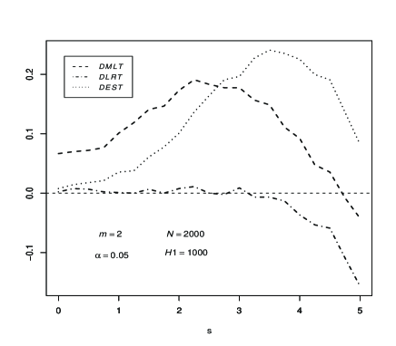
Refer to caption
Figure 10: ΔP𝒦e(s)Δsubscript𝑃𝒦𝑒𝑠\Delta P_{{\cal K}e}(s)  von Mises-Fisher
Refer to caption
Figure 11: ΔP𝒦e(s)Δsubscript𝑃𝒦𝑒𝑠\Delta P_{{\cal K}e}(s)  hyperboloid

Next the power function of the sequential m𝑚m-flat k𝑘k-test is evaluated in the two dimensional case m=2𝑚2m=2. Again we take 20 values of the distance s𝑠s from 0 to 5, and for each value of s𝑠s, we select the number of H1subscript𝐻1H_{1} equally spaced alternatives. The empirical average power P~𝒦e(s)subscript~𝑃superscript𝒦𝑒𝑠\tilde{P}_{{\cal K}^{*}e}(s) of the sequential m𝑚m-flat k=(0,0)superscript𝑘00k^{*}=(0,0)-test is calculated as the number of rejections relative to the number of H1subscript𝐻1H_{1}. This empirical average power P~𝒦e(s)subscript~𝑃superscript𝒦𝑒𝑠\tilde{P}_{{\cal K}^{*}e}(s) is compared with the nonsequential empirical average powers P𝒦e(s)subscript𝑃𝒦𝑒𝑠P_{{\cal K}e}(s) of MLT,LRT,EST𝑀𝐿𝑇𝐿𝑅𝑇𝐸𝑆𝑇MLT,\ LRT,\ EST. The stopping time τ𝜏\tau for the sequential test is determined by (6.6)

τ=inf{n|1mt=1nabl1(x(t),u^mle,n)gab(u^mle,n)Kν(u^mle,n)+c(u^mle,n)},𝜏infimumconditional-set𝑛1𝑚superscriptsubscript𝑡1𝑛subscript𝑎subscript𝑏subscript𝑙1𝑥𝑡subscript^𝑢𝑚𝑙𝑒𝑛superscript𝑔𝑎𝑏subscript^𝑢𝑚𝑙𝑒𝑛𝐾𝜈subscript^𝑢𝑚𝑙𝑒𝑛𝑐subscript^𝑢𝑚𝑙𝑒𝑛\displaystyle\tau=\inf\left\{n\ \Big{|}\ -\frac{1}{m}\sum_{t=1}^{n}\partial_{a}\partial_{b}l_{1}(x(t),{\hat{u}}_{mle,n})g^{ab}({\hat{u}}_{mle,n})\geq K\nu({\hat{u}}_{mle,n})+c({\hat{u}}_{mle,n})\right\},
c(u)=12(mrr1r2):von Mises-Fisherc(u)=12(mrr1r2):hyperboloid.:𝑐𝑢12𝑚𝑟superscript𝑟1superscript𝑟absent2von Mises-Fisher𝑐𝑢12𝑚𝑟superscript𝑟1superscript𝑟absent2:hyperboloid\displaystyle c(u)=-\frac{1}{2}\Big{(}\frac{m}{rr^{\dagger}}-\frac{1}{r^{\dagger 2}}\Big{)}\ :\ \textrm{von Mises-Fisher}\quad c(u)=-\frac{1}{2}\Big{(}-\frac{m}{rr^{\dagger}}-\frac{1}{r^{\dagger 2}}\Big{)}\ :\ \textrm{hyperboloid}.

Then the rejection region of the sequential m𝑚m-flat k=(0,0)superscript𝑘00k^{*}=(0,0)-test is given by (6.3)

R~M~c={u~ν|ga~b~(u0)u~ν0a~u~ν0b~(c0+ϵ~)2},u~ν0a~=Kν0[u~ν,mle,τa~u~νa~(u0)].formulae-sequencesubscript~𝑅subscript~𝑀𝑐conditional-setsubscript~𝑢𝜈subscript𝑔~𝑎~𝑏subscript𝑢0superscriptsubscript~𝑢𝜈0~𝑎superscriptsubscript~𝑢𝜈0~𝑏superscriptsubscript𝑐0~italic-ϵ2superscriptsubscript~𝑢𝜈0~𝑎𝐾subscript𝜈0delimited-[]subscriptsuperscript~𝑢~𝑎𝜈𝑚𝑙𝑒𝜏superscriptsubscript~𝑢𝜈~𝑎subscript𝑢0\displaystyle\tilde{R}_{\tilde{M}_{c}}=\left\{\tilde{u}_{\nu}\ \big{|}\ g_{\tilde{a}\tilde{b}}(u_{0})\tilde{u}_{\nu 0}^{\tilde{a}}\tilde{u}_{\nu 0}^{\tilde{b}}\geq(c_{0}+\tilde{\epsilon})^{2}\right\},\quad\tilde{u}_{\nu 0}^{\tilde{a}}=\sqrt{K\nu_{0}}\left[\tilde{u}^{\tilde{a}}_{\nu,mle,\tau}-\tilde{u}_{\nu}^{\tilde{a}}(u_{0})\right].

As for the von Mises-Fisher model, numerical results are based on the following set of values (cf. (7.1))

m=2,α=0.05,r=0.2,H0:(u01,u02)=(π/2,π/2),N=1000,H1=500,:formulae-sequence𝑚2formulae-sequence𝛼0.05𝑟0.2subscript𝐻0formulae-sequencesuperscriptsubscript𝑢01superscriptsubscript𝑢02𝜋2𝜋2formulae-sequence𝑁1000subscript𝐻1500\displaystyle m=2,\quad\alpha=0.05,\quad r=0.2,\quad H_{0}\ :\ (u_{0}^{1},u_{0}^{2})=(\pi/2,\pi/2),\quad N=1000,\quad H_{1}=500,
u~ν1=ν(u)η1(u),u~ν2=ν(u)η2(u),ν(u)=1/|sinu1||sinu2|,K=1000,formulae-sequencesuperscriptsubscript~𝑢𝜈1𝜈𝑢subscript𝜂1𝑢formulae-sequencesuperscriptsubscript~𝑢𝜈2𝜈𝑢subscript𝜂2𝑢formulae-sequence𝜈𝑢1superscript𝑢1superscript𝑢2𝐾1000\displaystyle\tilde{u}_{\nu}^{1}=\nu(u)\eta_{1}(u),\quad\tilde{u}_{\nu}^{2}=\nu(u)\eta_{2}(u),\quad\nu(u)=1/|\sin u^{1}||\sin u^{2}|,\qquad K=1000,

and for the hyperboloid model, numerical results are based on the following set of values (cf. (7.2))

m=2,α=0.05,r=2,H0:(u01,u02)=(1,π/2),N=50,H1=500,:formulae-sequence𝑚2formulae-sequence𝛼0.05𝑟2subscript𝐻0formulae-sequencesuperscriptsubscript𝑢01superscriptsubscript𝑢021𝜋2formulae-sequence𝑁50subscript𝐻1500\displaystyle m=2,\quad\alpha=0.05,\quad r=2,\quad H_{0}\ :\ (u_{0}^{1},u_{0}^{2})=(1,\pi/2),\quad N=50,\quad H_{1}=500,
u~ν1=ν(u)η1(u),u~ν2=ν(u)η2(u),ν(u)=1/|sinhu1||sinu2|,K=60formulae-sequencesuperscriptsubscript~𝑢𝜈1𝜈𝑢subscript𝜂1𝑢formulae-sequencesuperscriptsubscript~𝑢𝜈2𝜈𝑢subscript𝜂2𝑢formulae-sequence𝜈𝑢1superscript𝑢1superscript𝑢2𝐾60\displaystyle\tilde{u}_{\nu}^{1}=\nu(u)\eta_{1}(u),\quad\tilde{u}_{\nu}^{2}=\nu(u)\eta_{2}(u),\quad\nu(u)=1/|\sinh u^{1}||\sin u^{2}|,\quad K=60

Figures 12, 13 show the von Mises-Fisher model, and Figures 14, 15 show the hyperboloid model. Figures 12, 14 depict P~𝒦e(s),P𝒦e(s)subscript~𝑃superscript𝒦𝑒𝑠subscript𝑃𝒦𝑒𝑠\tilde{P}_{{\cal K}^{*}e}(s),\ P_{{\cal K}e}(s), and the notations in the figures indicate the following tests.

CMLT(sequential):k=(0,0),OMLT(nonsequential):k=(0,0),:𝐶𝑀𝐿𝑇𝑠𝑒𝑞𝑢𝑒𝑛𝑡𝑖𝑎𝑙superscript𝑘00𝑂𝑀𝐿𝑇𝑛𝑜𝑛𝑠𝑒𝑞𝑢𝑒𝑛𝑡𝑖𝑎𝑙:𝑘00\displaystyle CMLT(sequential)\ :\ k^{*}=(0,0),\quad OMLT(nonsequential)\ :\ k=(0,0),
OLRT(nonsequential):k=(0.5,0.5),OEST(nonsequential):k=(1,1).:𝑂𝐿𝑅𝑇𝑛𝑜𝑛𝑠𝑒𝑞𝑢𝑒𝑛𝑡𝑖𝑎𝑙𝑘0.50.5𝑂𝐸𝑆𝑇𝑛𝑜𝑛𝑠𝑒𝑞𝑢𝑒𝑛𝑡𝑖𝑎𝑙:𝑘11\displaystyle OLRT(nonsequential)\ :\ k=(0.5,0.5),\quad OEST(nonsequential)\ :\ k=(1,1).

Figures 13, 15 depict the differences DP𝒦e(s)=P~𝒦e(s)P𝒦e(s)𝐷subscript𝑃𝒦𝑒𝑠subscript~𝑃superscript𝒦𝑒𝑠subscript𝑃𝒦𝑒𝑠DP_{{\cal K}e}(s)=\tilde{P}_{{\cal K}^{*}e}(s)-P_{{\cal K}e}(s), and the notations in the figures indicate the following tests.

DMLT:k=(0,0),DLRT:k=(0.5,0.5),DEST:k=(1,1).:𝐷𝑀𝐿𝑇𝑘00𝐷𝐿𝑅𝑇:𝑘0.50.5𝐷𝐸𝑆𝑇:𝑘11\displaystyle DMLT\ :\ k=(0,0),\quad DLRT\ :\ k=(0.5,0.5),\quad DEST\ :\ k=(1,1).

We see that in each model, the empirical average power P~𝒦e(s)subscript~𝑃superscript𝒦𝑒𝑠\tilde{P}_{{\cal K}^{*}e}(s) of the sequential m𝑚m-flat k=(0,0)superscript𝑘00k^{*}=(0,0)-test (CMLT)𝐶𝑀𝐿𝑇(CMLT) surpasses the empirical average powers P𝒦e(s)subscript𝑃𝒦𝑒𝑠P_{{\cal K}e}(s) of typical nonsequential m𝑚m-flat k𝑘k-tests (OMLT,OLRT,OEST)𝑂𝑀𝐿𝑇𝑂𝐿𝑅𝑇𝑂𝐸𝑆𝑇(OMLT,\ OLRT,\ OEST) almost uniformly in the distance s>0𝑠0s>0.

Refer to caption
Figure 12: P~𝒦e(s),P𝒦e(s)subscript~𝑃superscript𝒦𝑒𝑠subscript𝑃𝒦𝑒𝑠\tilde{P}_{{\cal K}^{*}e}(s),P_{{\cal K}e}(s)  von Mises-Fisher
Refer to caption
Figure 13: DP𝒦e(s)𝐷subscript𝑃𝒦𝑒𝑠DP_{{\cal K}e}(s)  von Mises-Fisher
Refer to caption
Figure 14: P~𝒦e(s),P𝒦e(s)subscript~𝑃superscript𝒦𝑒𝑠subscript𝑃𝒦𝑒𝑠\tilde{P}_{{\cal K}^{*}e}(s),P_{{\cal K}e}(s)  hyperboloid
Refer to caption
Figure 15: DP𝒦e(s)𝐷subscript𝑃𝒦𝑒𝑠DP_{{\cal K}e}(s)  hyperboloid

8 DISCUSSION

Conformal geometry of statistical manifold has produced the concrete third-order efficient sequential test procedure in a multidimensional curved exponential family Mcsubscript𝑀𝑐M_{c}. The method is divided into two stages: the first is to choose the stopping rule which reduces the mean 1-ES curvature of the conformally transformed M~csubscript~𝑀𝑐\tilde{M}_{c} to zero, and the second is to determine the significance of the null hypothesis based on the mixture-flat k𝑘k-test statistic at the stopping time.

This method was also designed to verify that the totally exponential umbilic statistical manifold (TEU for short) guarantees the third-order uniformly efficient sequential test procedure. TEU implies the conformal mixture (exponential) flatness, and this flatness leads to a gauge function ν(u)>0𝜈𝑢0\nu(u)>0 and a dual affine coordinate system of M~csubscript~𝑀𝑐\tilde{M}_{c} which reduces the (1)1(-1)-connection of M~csubscript~𝑀𝑐\tilde{M}_{c} to zero. This coordinate system is not pertinent to the power function itself but is effective for the simplification of the sequential mixture-flat k𝑘k-test statistic without the bias-correction. Therefore TEU can be regarded as an f.r.m. exponential family in the appropriate sequential inferential procedure. The von-Mises Fisher model and the hyperboloid model are the examples of the dual quadric hypersurface which was coined in the previous work (Kumon et al., 2011). This type of hypersurface belongs to the class of TEU, and the complete characterization of TEU remains a future subject.

The present and the previous works exhibit one feature of active information geometry which encompasses geometries not only as interpretations but as strategic actions. It has been recognized that the sequential inferential procedures are rather restrictive in the sense that they cannot reduce the anisotoropy of statistical manifold. Another feature of the proposed spirit can be found in the field of dynamical systems, where dynamical actions such as feedback and feedforward may produce more flexible geometrical actions on system manifolds. This is a promising theme which is to be studied in a future work.

APPENDICES

1  Edgeworth expansion of f(w^,u)𝑓^𝑤𝑢f(\hat{w},u)

The observed sufficient statistic x¯¯𝑥\bar{x} is decomposed into (u^,v^)^𝑢^𝑣(\hat{u},\hat{v}) by x¯=η(u^,v^)¯𝑥𝜂^𝑢^𝑣\bar{x}=\eta(\hat{u},\hat{v}), implying that x¯¯𝑥\bar{x} is in the ancillary subspace A(u^)𝐴^𝑢A(\hat{u}) and its coordinates are v^^𝑣\hat{v} in A(u^)𝐴^𝑢A(\hat{u}). Then we define the normalized and bias-corrected statistics u~s,esuperscriptsubscript~𝑢𝑠𝑒\tilde{u}_{s,e}^{*} and v~~𝑣\tilde{v} by

u~s,e=N(u^us,e),u~s,ea=u~s,ea+12NΓβγ(1)agβγ(u^),v~=Nv^,formulae-sequencesubscript~𝑢𝑠𝑒𝑁^𝑢subscript𝑢𝑠𝑒formulae-sequencesuperscriptsubscript~𝑢𝑠𝑒absent𝑎superscriptsubscript~𝑢𝑠𝑒𝑎12𝑁superscriptsubscriptΓ𝛽𝛾1𝑎superscript𝑔𝛽𝛾^𝑢~𝑣𝑁^𝑣\displaystyle\tilde{u}_{s,e}=\sqrt{N}(\hat{u}-u_{s,e}),\quad\tilde{u}_{s,e}^{*a}=\tilde{u}_{s,e}^{a}+\frac{1}{2\sqrt{N}}\Gamma_{\beta\gamma}^{(-1)a}g^{\beta\gamma}(\hat{u}),\quad\tilde{v}=\sqrt{N}\hat{v},

and denote them by w~s,e=(u~s,e,v~)superscriptsubscript~𝑤𝑠𝑒superscriptsubscript~𝑢𝑠𝑒~𝑣\tilde{w}_{s,e}^{*}=(\tilde{u}_{s,e}^{*},\tilde{v}). The density functions of the statistics w~s,esuperscriptsubscript~𝑤𝑠𝑒\tilde{w}_{s,e}^{*} and u~s,esuperscriptsubscript~𝑢𝑠𝑒\tilde{u}_{s,e}^{*} are given in Amari and Kumon (1983), and we only enumerate the results.

When the true parameter is us,esubscript𝑢𝑠𝑒u_{s,e}, the density function f(w~s,e;us,e)𝑓superscriptsubscript~𝑤𝑠𝑒subscript𝑢𝑠𝑒f(\tilde{w}_{s,e}^{*};u_{s,e}) is expanded as

f(w~s,e;us,e)=|gαβ(us,e)|1/2(2π)n/2exp{12gαβ(us,e)w~s,eαw~s,eβ}+O(N1/2).𝑓superscriptsubscript~𝑤𝑠𝑒subscript𝑢𝑠𝑒superscriptsubscript𝑔𝛼𝛽subscript𝑢𝑠𝑒12superscript2𝜋𝑛212subscript𝑔𝛼𝛽subscript𝑢𝑠𝑒superscriptsubscript~𝑤𝑠𝑒absent𝛼superscriptsubscript~𝑤𝑠𝑒absent𝛽𝑂superscript𝑁12\displaystyle f(\tilde{w}_{s,e}^{*};u_{s,e})=\frac{|g_{\alpha\beta}(u_{s,e})|^{1/2}}{(2\pi)^{n/2}}\exp\left\{-\frac{1}{2}g_{\alpha\beta}(u_{s,e})\tilde{w}_{s,e}^{*\alpha}\tilde{w}_{s,e}^{*\beta}\right\}+O(N^{-1/2}). (8.1)

The distribution of u~s,esuperscriptsubscript~𝑢𝑠𝑒\tilde{u}_{s,e}^{*} is obtained by integrating (8.1) with respect to v~~𝑣\tilde{v},

f(u~s,e;us,e)=|g¯ab(us,e)|1/2(2π)m/2exp{12g¯ab(us,e)u~s,eau~s,eb}+O(N1/2),𝑓superscriptsubscript~𝑢𝑠𝑒subscript𝑢𝑠𝑒superscriptsubscript¯𝑔𝑎𝑏subscript𝑢𝑠𝑒12superscript2𝜋𝑚212subscript¯𝑔𝑎𝑏subscript𝑢𝑠𝑒superscriptsubscript~𝑢𝑠𝑒absent𝑎superscriptsubscript~𝑢𝑠𝑒absent𝑏𝑂superscript𝑁12\displaystyle f(\tilde{u}_{s,e}^{*};u_{s,e})=\frac{|\bar{g}_{ab}(u_{s,e})|^{1/2}}{(2\pi)^{m/2}}\exp\left\{-\frac{1}{2}\bar{g}_{ab}(u_{s,e})\tilde{u}_{s,e}^{*a}\tilde{u}_{s,e}^{*b}\right\}+O(N^{-1/2}), (8.2)

where

g¯ab(us,e)=gab(us,e)gaκgbλgκλ.subscript¯𝑔𝑎𝑏subscript𝑢𝑠𝑒subscript𝑔𝑎𝑏subscript𝑢𝑠𝑒subscript𝑔𝑎𝜅subscript𝑔𝑏𝜆superscript𝑔𝜅𝜆\displaystyle\bar{g}_{ab}(u_{s,e})=g_{ab}(u_{s,e})-g_{a\kappa}g_{b\lambda}g^{\kappa\lambda}. (8.3)

The matrix gabg¯absubscript𝑔𝑎𝑏subscript¯𝑔𝑎𝑏g_{ab}-\bar{g}_{ab} is positive semi-definite, and g¯ab(us,e)=gab(us,e)subscript¯𝑔𝑎𝑏subscript𝑢𝑠𝑒subscript𝑔𝑎𝑏subscript𝑢𝑠𝑒\bar{g}_{ab}(u_{s,e})=g_{ab}(u_{s,e}) holds if and only if gaκ(us,e)=0subscript𝑔𝑎𝜅subscript𝑢𝑠𝑒0g_{a\kappa}(u_{s,e})=0, that is, A𝐴A is orthogonal at us,esubscript𝑢𝑠𝑒u_{s,e}.

When A𝐴A is locally orthogonal at u0subscript𝑢0u_{0}, the density function of u~s,esuperscriptsubscript~𝑢𝑠𝑒\tilde{u}_{s,e}^{*} is further expanded as

f(u~s,e;us,e)=φ(u~s,e;us,e)[1+AN(u~s,e;us,e)+BN(u~s,e;us,e)]+O(N3/2),𝑓superscriptsubscript~𝑢𝑠𝑒subscript𝑢𝑠𝑒𝜑superscriptsubscript~𝑢𝑠𝑒subscript𝑢𝑠𝑒delimited-[]1subscript𝐴𝑁superscriptsubscript~𝑢𝑠𝑒subscript𝑢𝑠𝑒subscript𝐵𝑁superscriptsubscript~𝑢𝑠𝑒subscript𝑢𝑠𝑒𝑂superscript𝑁32\displaystyle f(\tilde{u}_{s,e}^{*};u_{s,e})=\varphi(\tilde{u}_{s,e}^{*};u_{s,e})\left[1+A_{N}(\tilde{u}_{s,e}^{*};u_{s,e})+B_{N}(\tilde{u}_{s,e}^{*};u_{s,e})\right]+O(N^{-3/2}), (8.4)

where

φ(u~s,e;us,e)=|gab(us,e)|1/2(2π)m/2exp{12gab(us,e)u~s,eau~s,eb},𝜑superscriptsubscript~𝑢𝑠𝑒subscript𝑢𝑠𝑒superscriptsubscript𝑔𝑎𝑏subscript𝑢𝑠𝑒12superscript2𝜋𝑚212subscript𝑔𝑎𝑏subscript𝑢𝑠𝑒superscriptsubscript~𝑢𝑠𝑒absent𝑎superscriptsubscript~𝑢𝑠𝑒absent𝑏\displaystyle\varphi(\tilde{u}_{s,e}^{*};u_{s,e})=\frac{|g_{ab}(u_{s,e})|^{1/2}}{(2\pi)^{m/2}}\exp\left\{-\frac{1}{2}g_{ab}(u_{s,e})\tilde{u}_{s,e}^{*a}\tilde{u}_{s,e}^{*b}\right\}, (8.5)
AN(u~s,e;us,e)=16NKabchabcsubscript𝐴𝑁superscriptsubscript~𝑢𝑠𝑒subscript𝑢𝑠𝑒16𝑁subscript𝐾𝑎𝑏𝑐superscript𝑎𝑏𝑐\displaystyle A_{N}(\tilde{u}_{s,e}^{*};u_{s,e})=\frac{1}{6\sqrt{N}}K_{abc}h^{abc}
+14NKabhab+124NKabcdhabcd+172NKabcKdefhabcdef,14𝑁subscript𝐾𝑎𝑏superscript𝑎𝑏124𝑁subscript𝐾𝑎𝑏𝑐𝑑superscript𝑎𝑏𝑐𝑑172𝑁subscript𝐾𝑎𝑏𝑐subscript𝐾𝑑𝑒𝑓superscript𝑎𝑏𝑐𝑑𝑒𝑓\displaystyle\qquad\qquad\qquad\ \ +\frac{1}{4N}K_{ab}h^{ab}+\frac{1}{24N}K_{abcd}h^{abcd}+\frac{1}{72N}K_{abc}K_{def}h^{abcdef}, (8.6)
Kabc=Tabc3Cabc,subscript𝐾𝑎𝑏𝑐subscript𝑇𝑎𝑏𝑐3subscript𝐶𝑎𝑏𝑐\displaystyle K_{abc}=T_{abc}-3C_{abc},
Kab=CcdaCefdgcegdf+2Hacκ(1)Hbdλ(1)gcdgκλ,subscript𝐾𝑎𝑏subscript𝐶𝑐𝑑𝑎subscript𝐶𝑒𝑓𝑑superscript𝑔𝑐𝑒superscript𝑔𝑑𝑓2superscriptsubscript𝐻𝑎𝑐𝜅1superscriptsubscript𝐻𝑏𝑑𝜆1superscript𝑔𝑐𝑑superscript𝑔𝜅𝜆\displaystyle K_{ab}=C_{cda}C_{efd}g^{ce}g^{df}+2H_{ac\kappa}^{(1)}H_{bd\lambda}^{(1)}g^{cd}g^{\kappa\lambda},
Kabcd=Sabcd4Dabcd+12(Ceab+CabeTabe)Cfcdgef,subscript𝐾𝑎𝑏𝑐𝑑subscript𝑆𝑎𝑏𝑐𝑑4subscript𝐷𝑎𝑏𝑐𝑑12subscript𝐶𝑒𝑎𝑏subscript𝐶𝑎𝑏𝑒subscript𝑇𝑎𝑏𝑒subscript𝐶𝑓𝑐𝑑superscript𝑔𝑒𝑓\displaystyle K_{abcd}=S_{abcd}-4D_{abcd}+12(C_{eab}+C_{abe}-T_{abe})C_{fcd}g^{ef},
Tabc=TijkBaiBbjBck,Cabc=bBaiBci=Γabc(1),formulae-sequencesubscript𝑇𝑎𝑏𝑐subscript𝑇𝑖𝑗𝑘superscriptsubscript𝐵𝑎𝑖superscriptsubscript𝐵𝑏𝑗superscriptsubscript𝐵𝑐𝑘subscript𝐶𝑎𝑏𝑐subscript𝑏subscript𝐵𝑎𝑖superscriptsubscript𝐵𝑐𝑖superscriptsubscriptΓ𝑎𝑏𝑐1\displaystyle T_{abc}=T_{ijk}B_{a}^{i}B_{b}^{j}B_{c}^{k},\quad C_{abc}=\partial_{b}B_{ai}B_{c}^{i}=\Gamma_{abc}^{(-1)},
Sabcd=ijklψBaiBbjBckBdl,Dabcd=cbBaiBdi,formulae-sequencesubscript𝑆𝑎𝑏𝑐𝑑subscript𝑖subscript𝑗subscript𝑘subscript𝑙𝜓superscriptsubscript𝐵𝑎𝑖superscriptsubscript𝐵𝑏𝑗superscriptsubscript𝐵𝑐𝑘superscriptsubscript𝐵𝑑𝑙subscript𝐷𝑎𝑏𝑐𝑑subscript𝑐subscript𝑏subscript𝐵𝑎𝑖superscriptsubscript𝐵𝑑𝑖\displaystyle S_{abcd}=\partial_{i}\partial_{j}\partial_{k}\partial_{l}\psi B_{a}^{i}B_{b}^{j}B_{c}^{k}B_{d}^{l},\quad D_{abcd}=\partial_{c}\partial_{b}B_{ai}B_{d}^{i},
2NBN(u~s,e;us,e)=[Qacκ{(gac+s2eaec)Qbdλ2gacHbdλ(1)}gκλ+12Hab(1)2]hab2𝑁subscript𝐵𝑁superscriptsubscript~𝑢𝑠𝑒subscript𝑢𝑠𝑒delimited-[]subscript𝑄𝑎𝑐𝜅superscript𝑔𝑎𝑐superscript𝑠2superscript𝑒𝑎superscript𝑒𝑐subscript𝑄𝑏𝑑𝜆2superscript𝑔𝑎𝑐superscriptsubscript𝐻𝑏𝑑𝜆1superscript𝑔𝜅𝜆12superscriptsubscript𝐻𝑎𝑏12superscript𝑎𝑏\displaystyle 2NB_{N}(\tilde{u}_{s,e}^{*};u_{s,e})=\left[Q_{ac\kappa}\left\{\left(g^{ac}+s^{2}e^{a}e^{c}\right)Q_{bd\lambda}-2g^{ac}H_{bd\lambda}^{(1)}\right\}g^{\kappa\lambda}+\frac{1}{2}H_{ab}^{(-1)2}\right]h^{ab}
+sQcdλ(2QabκHabκ(1))gκλedhabc+Qabκ(QcdλHcdλ(1))gκλhabcd,𝑠subscript𝑄𝑐𝑑𝜆2subscript𝑄𝑎𝑏𝜅superscriptsubscript𝐻𝑎𝑏𝜅1superscript𝑔𝜅𝜆superscript𝑒𝑑superscript𝑎𝑏𝑐subscript𝑄𝑎𝑏𝜅subscript𝑄𝑐𝑑𝜆superscriptsubscript𝐻𝑐𝑑𝜆1superscript𝑔𝜅𝜆superscript𝑎𝑏𝑐𝑑\displaystyle\qquad\qquad\qquad\qquad\ +sQ_{cd\lambda}\left(2Q_{ab\kappa}-H_{ab\kappa}^{(1)}\right)g^{\kappa\lambda}e^{d}h^{abc}+Q_{ab\kappa}\left(Q_{cd\lambda}-H_{cd\lambda}^{(1)}\right)g^{\kappa\lambda}h^{abcd}, (8.7)
Hab(1)2=Hκλa(1)Hμνb(1)gκμgλν,superscriptsubscript𝐻𝑎𝑏12superscriptsubscript𝐻𝜅𝜆𝑎1superscriptsubscript𝐻𝜇𝜈𝑏1superscript𝑔𝜅𝜇superscript𝑔𝜆𝜈\displaystyle H_{ab}^{(-1)2}=H_{\kappa\lambda a}^{(-1)}H_{\mu\nu b}^{(-1)}g^{\kappa\mu}g^{\lambda\nu},

and habsuperscript𝑎𝑏h^{ab} etc. are the tensorial Hermite polynomials in u~s,esubscript~𝑢𝑠𝑒\tilde{u}_{s,e} as follows.

hab(u)=uaubgab,habc(u)=uaubuc3g(abuc),\displaystyle h^{ab}(u)=u^{a}u^{b}-g^{ab},\quad h^{abc}(u)=u^{a}u^{b}u^{c}-3g^{(ab}u^{c)},
habcd(u)=uaubucud6g(abucud)+3g(abgcd),\displaystyle h^{abcd}(u)=u^{a}u^{b}u^{c}u^{d}-6g^{(ab}u^{c}u^{d)}+3g^{(ab}g^{cd)},
habcdef(u)=uaubucudueuf15g(abucudueuf)+45g(abgcdueuf)15g(abgcdgef).\displaystyle h^{abcdef}(u)=u^{a}u^{b}u^{c}u^{d}u^{e}u^{f}-15g^{(ab}u^{c}u^{d}u^{e}u^{f)}+45g^{(ab}g^{cd}u^{e}u^{f)}-15g^{(ab}g^{cd}g^{ef)}.

The term AN(u~s,e;us,e)subscript𝐴𝑁superscriptsubscript~𝑢𝑠𝑒subscript𝑢𝑠𝑒A_{N}(\tilde{u}_{s,e}^{*};u_{s,e}) does not depend on the ancillary family A𝐴A, so that it is common to all the efficient tests. The term BN(u~s,e;us,e)subscript𝐵𝑁superscriptsubscript~𝑢𝑠𝑒subscript𝑢𝑠𝑒B_{N}(\tilde{u}_{s,e}^{*};u_{s,e}) shows that the density function f(u~s,e;us,e)𝑓superscriptsubscript~𝑢𝑠𝑒subscript𝑢𝑠𝑒f(\tilde{u}_{s,e}^{*};u_{s,e}) depends on A𝐴A through the two geometrical quantities Qabκsubscript𝑄𝑎𝑏𝜅Q_{ab\kappa} and Hκλa(1)superscriptsubscript𝐻𝜅𝜆𝑎1H_{\kappa\lambda a}^{(-1)}. Thus when A𝐴A is associated with a test, the third-order characteristics of an efficient test are determined by the angles Qabκsubscript𝑄𝑎𝑏𝜅Q_{ab\kappa} between the boundary R𝑅\partial R of the critical region R𝑅R and Mcsubscript𝑀𝑐M_{c}, and the (1)1(-1)-ES curvature Hκλa(1)superscriptsubscript𝐻𝜅𝜆𝑎1H_{\kappa\lambda a}^{(-1)} of R𝑅\partial R.

2  Outline on the second- and third-order powers

From the third-order level condition P𝒯(0)=α+O(N3/2)subscript𝑃𝒯0𝛼𝑂superscript𝑁32P_{{\cal T}}(0)=\alpha+O(N^{-3/2}), we have

R¯Mcf(u~0;u0)𝑑u~0+ϵf(u~0;u0)R¯Mc=1α,R¯Mc={u0~|gab(u0)u~0au~0bc02},formulae-sequencesubscriptsuperscriptsubscript¯𝑅subscript𝑀𝑐𝑓subscript~𝑢0subscript𝑢0differential-dsubscript~𝑢0italic-ϵsubscriptdelimited-⟨⟩𝑓subscript~𝑢0subscript𝑢0superscriptsubscript¯𝑅subscript𝑀𝑐1𝛼superscriptsubscript¯𝑅subscript𝑀𝑐conditional-set~subscript𝑢0subscript𝑔𝑎𝑏subscript𝑢0superscriptsubscript~𝑢0𝑎superscriptsubscript~𝑢0𝑏superscriptsubscript𝑐02\displaystyle\int_{\bar{R}_{M_{c}}^{*}}f(\tilde{u}_{0};u_{0})\ d\tilde{u}_{0}+\epsilon\langle f(\tilde{u}_{0};u_{0})\rangle_{\partial\bar{R}_{M_{c}}^{*}}=1-\alpha,\quad\bar{R}_{M_{c}}^{*}=\{\tilde{u_{0}}\ |\ g_{ab}(u_{0})\tilde{u}_{0}^{a}\tilde{u}_{0}^{b}\leq c_{0}^{2}\},
f(u~0;u0)R¯Mc=R¯Mcf(u~0;u0)𝑑u~0/SN(R¯Mc),R¯Mc={u0~|gab(u0)u~0au~0b=c02},formulae-sequencesubscriptdelimited-⟨⟩𝑓subscript~𝑢0subscript𝑢0superscriptsubscript¯𝑅subscript𝑀𝑐subscriptsuperscriptsubscript¯𝑅subscript𝑀𝑐𝑓subscript~𝑢0subscript𝑢0differential-dsubscript~𝑢0subscript𝑆𝑁superscriptsubscript¯𝑅subscript𝑀𝑐superscriptsubscript¯𝑅subscript𝑀𝑐conditional-set~subscript𝑢0subscript𝑔𝑎𝑏subscript𝑢0superscriptsubscript~𝑢0𝑎superscriptsubscript~𝑢0𝑏superscriptsubscript𝑐02\displaystyle\langle f(\tilde{u}_{0};u_{0})\rangle_{\partial\bar{R}_{M_{c}}^{*}}=\int_{\partial\bar{R}_{M_{c}}^{*}}f(\tilde{u}_{0};u_{0})\ d\tilde{u}_{0}/S_{N}(\partial\bar{R}_{M_{c}}^{*}),\quad\partial\bar{R}_{M_{c}}^{*}=\{\tilde{u_{0}}\ |\ g_{ab}(u_{0})\tilde{u}_{0}^{a}\tilde{u}_{0}^{b}=c_{0}^{2}\},

where SN(R¯Mc)subscript𝑆𝑁superscriptsubscript¯𝑅subscript𝑀𝑐S_{N}(\partial\bar{R}_{M_{c}}^{*}) denotes the area of the (m1)𝑚1(m-1)-dimensional sphere R¯Mcsuperscriptsubscript¯𝑅subscript𝑀𝑐\partial\bar{R}_{M_{c}}^{*} with the radius c0subscript𝑐0c_{0}.

We denote by ϵ0subscriptitalic-ϵ0\epsilon_{0} for the m.l.e. test, and for a general efficient test, we put ϵ=ϵ0+ϵ1italic-ϵsubscriptitalic-ϵ0subscriptitalic-ϵ1\epsilon=\epsilon_{0}+\epsilon_{1}. Then from the expression of AN(u~0;u0)subscript𝐴𝑁superscriptsubscript~𝑢0subscript𝑢0A_{N}(\tilde{u}_{0}^{*};u_{0}) given by (8) we have for ϵ0subscriptitalic-ϵ0\epsilon_{0}

Nϵ0=14mKabgabh1(c0)+124m(m+2)Kabcd3g(abgcd)h3(c0)\displaystyle N\epsilon_{0}=\frac{1}{4m}K_{ab}g^{ab}h_{1}(c_{0})+\frac{1}{24m(m+2)}K_{abcd}3g^{(ab}g^{cd)}h_{3}(c_{0})
+172m(m+2)(m+4)KabcKdef15g(abgcdgef)h5(c0),\displaystyle\qquad\quad+\frac{1}{72m(m+2)(m+4)}K_{abc}K_{def}15g^{(ab}g^{cd}g^{ef)}h_{5}(c_{0}),
h1(c0)=c0,h3(c0)=c03(m+2)c0,h5(c0)=c052(m+4)c03+(m+2)(m+4)c0.formulae-sequencesubscript1subscript𝑐0subscript𝑐0formulae-sequencesubscript3subscript𝑐0superscriptsubscript𝑐03𝑚2subscript𝑐0subscript5subscript𝑐0superscriptsubscript𝑐052𝑚4superscriptsubscript𝑐03𝑚2𝑚4subscript𝑐0\displaystyle h_{1}(c_{0})=c_{0},\quad h_{3}(c_{0})=c_{0}^{3}-(m+2)c_{0},\quad h_{5}(c_{0})=c_{0}^{5}-2(m+4)c_{0}^{3}+(m+2)(m+4)c_{0}.

On the other hand, from the expression of BN(u~0;u0)subscript𝐵𝑁superscriptsubscript~𝑢0subscript𝑢0B_{N}(\tilde{u}_{0}^{*};u_{0}) given by (8) we have for ϵ1subscriptitalic-ϵ1\epsilon_{1}

Nϵ1=[14mHA(1)2+12mQabκ(Qcdλ2Hcdλ(1))gacgbdgκλ]h1(c0)𝑁subscriptitalic-ϵ1delimited-[]14𝑚superscriptsubscript𝐻𝐴1212𝑚subscript𝑄𝑎𝑏𝜅subscript𝑄𝑐𝑑𝜆2superscriptsubscript𝐻𝑐𝑑𝜆1superscript𝑔𝑎𝑐superscript𝑔𝑏𝑑superscript𝑔𝜅𝜆subscript1subscript𝑐0\displaystyle N\epsilon_{1}=\left[\frac{1}{4m}H_{A}^{(-1)2}+\frac{1}{2m}Q_{ab\kappa}\left(Q_{cd\lambda}-2H_{cd\lambda}^{(1)}\right)g^{ac}g^{bd}g^{\kappa\lambda}\right]h_{1}(c_{0})
+[12m(m+2)Qabκ(QcdλHcdλ(1))g(abgcd)gκλ]h3(c0).\displaystyle\qquad\quad+\left[\frac{1}{2m(m+2)}Q_{ab\kappa}\left(Q_{cd\lambda}-H_{cd\lambda}^{(1)}\right)g^{(ab}g^{cd)}g^{\kappa\lambda}\right]h_{3}(c_{0}).

Since it needs long and complicated calculations to derive Proposition 3.2, we only enumerate key formulae on the integrations of the tensorial Hermite polynomials which were also used to get ϵ0,ϵ1subscriptitalic-ϵ0subscriptitalic-ϵ1\epsilon_{0},\epsilon_{1}.

R¯Mchabφ(u~s,e;us,e)du~s,ee=1mgabh1(c0),subscriptsuperscriptsubscript¯𝑅subscript𝑀𝑐subscriptdelimited-⟨⟩superscript𝑎𝑏𝜑superscriptsubscript~𝑢𝑠𝑒subscript𝑢𝑠𝑒𝑑superscriptsubscript~𝑢𝑠𝑒𝑒1𝑚superscript𝑔𝑎𝑏subscript1subscript𝑐0\displaystyle\int_{\bar{R}_{M_{c}}^{*}}\langle h^{ab}\varphi(\tilde{u}_{s,e}^{*};u_{s,e})\ d\tilde{u}_{s,e}^{*}\rangle_{e}=-\frac{1}{m}g^{ab}h_{1}(c_{0}),
R¯Mchabcdφ(u~s,e;us,e)du~s,ee=1m(m+2)3g(abgcd)h3(c0),\displaystyle\int_{\bar{R}_{M_{c}}^{*}}\langle h^{abcd}\varphi(\tilde{u}_{s,e}^{*};u_{s,e})\ d\tilde{u}_{s,e}^{*}\rangle_{e}=-\frac{1}{m(m+2)}3g^{(ab}g^{cd)}h_{3}(c_{0}),
R¯Mchabcdefφ(u~s,e;us,e)du~s,ee=1m(m+2)(m+4)15g(abgcdgef)h5(c0).\displaystyle\int_{\bar{R}_{M_{c}}^{*}}\langle h^{abcdef}\varphi(\tilde{u}_{s,e}^{*};u_{s,e})\ d\tilde{u}_{s,e}^{*}\rangle_{e}=-\frac{1}{m(m+2)(m+4)}15g^{(ab}g^{cd}g^{ef)}h_{5}(c_{0}).

3  Edgeworth expansion of f~(w^,u)~𝑓^𝑤𝑢\tilde{f}(\hat{w},u)

We define the normalized and bias-corrected statistics u~n,s,esuperscriptsubscript~𝑢𝑛𝑠𝑒\tilde{u}_{n,s,e}^{*} and v~nsubscript~𝑣𝑛\tilde{v}_{n} by

u~n,s,e=Kν0(u^nus,e),u~n,s,ea=u~n,s,ea+12Kν0Γ~βγ(1)agβγ(u^n),v~n=Kν0v^,formulae-sequencesubscript~𝑢𝑛𝑠𝑒𝐾subscript𝜈0subscript^𝑢𝑛subscript𝑢𝑠𝑒formulae-sequencesuperscriptsubscript~𝑢𝑛𝑠𝑒absent𝑎superscriptsubscript~𝑢𝑛𝑠𝑒𝑎12𝐾subscript𝜈0superscriptsubscript~Γ𝛽𝛾1𝑎superscript𝑔𝛽𝛾subscript^𝑢𝑛subscript~𝑣𝑛𝐾subscript𝜈0^𝑣\displaystyle\tilde{u}_{n,s,e}=\sqrt{K\nu_{0}}(\hat{u}_{n}-u_{s,e}),\quad\tilde{u}_{n,s,e}^{*a}=\tilde{u}_{n,s,e}^{a}+\frac{1}{2\sqrt{K\nu_{0}}}\tilde{\Gamma}_{\beta\gamma}^{(-1)a}g^{\beta\gamma}(\hat{u}_{n}),\quad\tilde{v}_{n}=\sqrt{K\nu_{0}}\hat{v},

and denote them by w~n,s,e=(u~n,s,e,v~n)superscriptsubscript~𝑤𝑛𝑠𝑒superscriptsubscript~𝑢𝑛𝑠𝑒subscript~𝑣𝑛\tilde{w}_{n,s,e}^{*}=(\tilde{u}_{n,s,e}^{*},\tilde{v}_{n}).

When the true parameter is us,esubscript𝑢𝑠𝑒u_{s,e}, the density function f~(w~n,s,e;us,e)~𝑓superscriptsubscript~𝑤𝑛𝑠𝑒subscript𝑢𝑠𝑒\tilde{f}(\tilde{w}_{n,s,e}^{*};u_{s,e}) of w~n,s,esuperscriptsubscript~𝑤𝑛𝑠𝑒\tilde{w}_{n,s,e}^{*} is expanded as

f~(w~n,s,e;us,e)=|gαβ(us,e)|1/2(2π)n/2exp{12gαβ(us,e)w~n,s,eαw~n,s,eβ}+O(K1/2).~𝑓superscriptsubscript~𝑤𝑛𝑠𝑒subscript𝑢𝑠𝑒superscriptsubscript𝑔𝛼𝛽subscript𝑢𝑠𝑒12superscript2𝜋𝑛212subscript𝑔𝛼𝛽subscript𝑢𝑠𝑒superscriptsubscript~𝑤𝑛𝑠𝑒absent𝛼superscriptsubscript~𝑤𝑛𝑠𝑒absent𝛽𝑂superscript𝐾12\displaystyle\tilde{f}(\tilde{w}_{n,s,e}^{*};u_{s,e})=\frac{|g_{\alpha\beta}(u_{s,e})|^{1/2}}{(2\pi)^{n/2}}\exp\left\{-\frac{1}{2}g_{\alpha\beta}(u_{s,e})\tilde{w}_{n,s,e}^{*\alpha}\tilde{w}_{n,s,e}^{*\beta}\right\}+O(K^{-1/2}). (8.8)

The distribution of u~n,s,esuperscriptsubscript~𝑢𝑛𝑠𝑒\tilde{u}_{n,s,e}^{*} is obtained by integrating (8.8) with respect to v~nsubscript~𝑣𝑛\tilde{v}_{n},

f~(u~n,s,e;us,e)=|g¯ab(us,e)|1/2(2π)m/2exp{12g¯ab(us,e)u~n,s,eau~n,s,eb}+O(K1/2),~𝑓superscriptsubscript~𝑢𝑛𝑠𝑒subscript𝑢𝑠𝑒superscriptsubscript¯𝑔𝑎𝑏subscript𝑢𝑠𝑒12superscript2𝜋𝑚212subscript¯𝑔𝑎𝑏subscript𝑢𝑠𝑒superscriptsubscript~𝑢𝑛𝑠𝑒absent𝑎superscriptsubscript~𝑢𝑛𝑠𝑒absent𝑏𝑂superscript𝐾12\displaystyle\tilde{f}(\tilde{u}_{n,s,e}^{*};u_{s,e})=\frac{|\bar{g}_{ab}(u_{s,e})|^{1/2}}{(2\pi)^{m/2}}\exp\left\{-\frac{1}{2}\bar{g}_{ab}(u_{s,e})\tilde{u}_{n,s,e}^{*a}\tilde{u}_{n,s,e}^{*b}\right\}+O(K^{-1/2}), (8.9)

where g¯ab(us,e)subscript¯𝑔𝑎𝑏subscript𝑢𝑠𝑒\bar{g}_{ab}(u_{s,e}) is the same as (8.3).

When A𝐴A is locally orthogonal at u0subscript𝑢0u_{0}, the density function of u~n,s,esuperscriptsubscript~𝑢𝑛𝑠𝑒\tilde{u}_{n,s,e}^{*} is further expanded as

f~(u~n,s,e;us,e)=φ(u~n,s,e;us,e)[1+A~K(u~n,s,e;us,e)+B~K(u~n,s,e;us,e)]+O(K3/2),~𝑓superscriptsubscript~𝑢𝑛𝑠𝑒subscript𝑢𝑠𝑒𝜑superscriptsubscript~𝑢𝑛𝑠𝑒subscript𝑢𝑠𝑒delimited-[]1subscript~𝐴𝐾superscriptsubscript~𝑢𝑛𝑠𝑒subscript𝑢𝑠𝑒subscript~𝐵𝐾superscriptsubscript~𝑢𝑛𝑠𝑒subscript𝑢𝑠𝑒𝑂superscript𝐾32\displaystyle\tilde{f}(\tilde{u}_{n,s,e}^{*};u_{s,e})=\varphi(\tilde{u}_{n,s,e}^{*};u_{s,e})\left[1+\tilde{A}_{K}(\tilde{u}_{n,s,e}^{*};u_{s,e})+\tilde{B}_{K}(\tilde{u}_{n,s,e}^{*};u_{s,e})\right]+O(K^{-3/2}), (8.10)

where

φ(u~n,s,e;us,e)=|gab(us,e)|1/2(2π)m/2exp{12gab(us,e)u~n,s,eau~n,s,eb},𝜑superscriptsubscript~𝑢𝑛𝑠𝑒subscript𝑢𝑠𝑒superscriptsubscript𝑔𝑎𝑏subscript𝑢𝑠𝑒12superscript2𝜋𝑚212subscript𝑔𝑎𝑏subscript𝑢𝑠𝑒superscriptsubscript~𝑢𝑛𝑠𝑒absent𝑎superscriptsubscript~𝑢𝑛𝑠𝑒absent𝑏\displaystyle\varphi(\tilde{u}_{n,s,e}^{*};u_{s,e})=\frac{|g_{ab}(u_{s,e})|^{1/2}}{(2\pi)^{m/2}}\exp\left\{-\frac{1}{2}g_{ab}(u_{s,e})\tilde{u}_{n,s,e}^{*a}\tilde{u}_{n,s,e}^{*b}\right\}, (8.11)
A~K(u~n,s,e;us,e)=16Kν0K~abchabcsubscript~𝐴𝐾superscriptsubscript~𝑢𝑛𝑠𝑒subscript𝑢𝑠𝑒16𝐾subscript𝜈0subscript~𝐾𝑎𝑏𝑐superscript𝑎𝑏𝑐\displaystyle\tilde{A}_{K}(\tilde{u}_{n,s,e}^{*};u_{s,e})=\frac{1}{6\sqrt{K\nu_{0}}}\tilde{K}_{abc}h^{abc}
+14Kν0K~abhab+124Kν0K~abcdhabcd+172Kν0K~abcK~defhabcdef,14𝐾subscript𝜈0subscript~𝐾𝑎𝑏superscript𝑎𝑏124𝐾subscript𝜈0subscript~𝐾𝑎𝑏𝑐𝑑superscript𝑎𝑏𝑐𝑑172𝐾subscript𝜈0subscript~𝐾𝑎𝑏𝑐subscript~𝐾𝑑𝑒𝑓superscript𝑎𝑏𝑐𝑑𝑒𝑓\displaystyle\qquad\qquad\qquad\ \ \ +\frac{1}{4K\nu_{0}}\tilde{K}_{ab}h^{ab}+\frac{1}{24K\nu_{0}}\tilde{K}_{abcd}h^{abcd}+\frac{1}{72K\nu_{0}}\tilde{K}_{abc}\tilde{K}_{def}h^{abcdef}, (8.12)
K~abc=T~abc3C~abc,subscript~𝐾𝑎𝑏𝑐subscript~𝑇𝑎𝑏𝑐3subscript~𝐶𝑎𝑏𝑐\displaystyle\tilde{K}_{abc}=\tilde{T}_{abc}-3\tilde{C}_{abc},
K~ab=C~cdaC~efdgcegdf+2H~acκ(1)H~bdλ(1)gcdgκλ,subscript~𝐾𝑎𝑏subscript~𝐶𝑐𝑑𝑎subscript~𝐶𝑒𝑓𝑑superscript𝑔𝑐𝑒superscript𝑔𝑑𝑓2superscriptsubscript~𝐻𝑎𝑐𝜅1superscriptsubscript~𝐻𝑏𝑑𝜆1superscript𝑔𝑐𝑑superscript𝑔𝜅𝜆\displaystyle\tilde{K}_{ab}=\tilde{C}_{cda}\tilde{C}_{efd}g^{ce}g^{df}+2\tilde{H}_{ac\kappa}^{(1)}\tilde{H}_{bd\lambda}^{(1)}g^{cd}g^{\kappa\lambda},
K~abcd=S~abcd4D~abcd+12(C~eab+C~abeT~abe)C~fcdgef,subscript~𝐾𝑎𝑏𝑐𝑑subscript~𝑆𝑎𝑏𝑐𝑑4subscript~𝐷𝑎𝑏𝑐𝑑12subscript~𝐶𝑒𝑎𝑏subscript~𝐶𝑎𝑏𝑒subscript~𝑇𝑎𝑏𝑒subscript~𝐶𝑓𝑐𝑑superscript𝑔𝑒𝑓\displaystyle\tilde{K}_{abcd}=\tilde{S}_{abcd}-4\tilde{D}_{abcd}+12(\tilde{C}_{eab}+\tilde{C}_{abe}-\tilde{T}_{abe})\tilde{C}_{fcd}g^{ef},
C~abc=Γ~abc(1),D~abcd=cC~abdC~abe(C~cdfT~cdf)gef,formulae-sequencesubscript~𝐶𝑎𝑏𝑐superscriptsubscript~Γ𝑎𝑏𝑐1subscript~𝐷𝑎𝑏𝑐𝑑subscript𝑐subscript~𝐶𝑎𝑏𝑑subscript~𝐶𝑎𝑏𝑒subscript~𝐶𝑐𝑑𝑓subscript~𝑇𝑐𝑑𝑓superscript𝑔𝑒𝑓\displaystyle\tilde{C}_{abc}=\tilde{\Gamma}_{abc}^{(-1)},\quad\tilde{D}_{abcd}=\partial_{c}\tilde{C}_{abd}-\tilde{C}_{abe}(\tilde{C}_{cdf}-\tilde{T}_{cdf})g^{ef},
S~abcd=Sabcd+6s(abgcd)+4s(aTbcd)+(1sαsβgαβ)3g(abgcd),sab=asb+sasbΓ~ab(1)csc,\displaystyle\tilde{S}_{abcd}=S_{abcd}+6s_{(ab}g_{cd)}+4s_{(a}T_{bcd)}+(1-s_{\alpha}s_{\beta}g^{\alpha\beta})3g_{(ab}g_{cd)},\quad s_{ab}=\partial_{a}s_{b}+s_{a}s_{b}-\tilde{\Gamma}_{ab}^{(1)c}s_{c},
2Kν0B~K(u~n,s,e;us,e)=[Q~acκ{(gac+s2eaec)Q~bdλ2gacH~bdλ(1)}gκλ+12Hab(1)2]hab2𝐾subscript𝜈0subscript~𝐵𝐾superscriptsubscript~𝑢𝑛𝑠𝑒subscript𝑢𝑠𝑒delimited-[]subscript~𝑄𝑎𝑐𝜅superscript𝑔𝑎𝑐superscript𝑠2superscript𝑒𝑎superscript𝑒𝑐subscript~𝑄𝑏𝑑𝜆2superscript𝑔𝑎𝑐superscriptsubscript~𝐻𝑏𝑑𝜆1superscript𝑔𝜅𝜆12superscriptsubscript𝐻𝑎𝑏12superscript𝑎𝑏\displaystyle 2K\nu_{0}\tilde{B}_{K}(\tilde{u}_{n,s,e}^{*};u_{s,e})=\left[\tilde{Q}_{ac\kappa}\left\{\left(g^{ac}+s^{2}e^{a}e^{c}\right)\tilde{Q}_{bd\lambda}-2g^{ac}\tilde{H}_{bd\lambda}^{(1)}\right\}g^{\kappa\lambda}+\frac{1}{2}H_{ab}^{(-1)2}\right]h^{ab}
+sQ~cdλ(2Q~abκH~abκ(1))gκλedhabc+Q~abκ(Q~cdλH~cdλ(1))gκλhabcd.𝑠subscript~𝑄𝑐𝑑𝜆2subscript~𝑄𝑎𝑏𝜅superscriptsubscript~𝐻𝑎𝑏𝜅1superscript𝑔𝜅𝜆superscript𝑒𝑑superscript𝑎𝑏𝑐subscript~𝑄𝑎𝑏𝜅subscript~𝑄𝑐𝑑𝜆superscriptsubscript~𝐻𝑐𝑑𝜆1superscript𝑔𝜅𝜆superscript𝑎𝑏𝑐𝑑\displaystyle\qquad\qquad\qquad\qquad\ +s\tilde{Q}_{cd\lambda}\left(2\tilde{Q}_{ab\kappa}-\tilde{H}_{ab\kappa}^{(1)}\right)g^{\kappa\lambda}e^{d}h^{abc}+\tilde{Q}_{ab\kappa}\left(\tilde{Q}_{cd\lambda}-\tilde{H}_{cd\lambda}^{(1)}\right)g^{\kappa\lambda}h^{abcd}. (8.13)

The term A~K(u~n,s,e;us,e)subscript~𝐴𝐾superscriptsubscript~𝑢𝑛𝑠𝑒subscript𝑢𝑠𝑒\tilde{A}_{K}(\tilde{u}_{n,s,e}^{*};u_{s,e}) does not depend on the ancillary family A~~𝐴\tilde{A}, so that it is common to all the efficient sequential tests. The term B~K(u~n,s,e;us,e)subscript~𝐵𝐾superscriptsubscript~𝑢𝑛𝑠𝑒subscript𝑢𝑠𝑒\tilde{B}_{K}(\tilde{u}_{n,s,e}^{*};u_{s,e}) shows that the density function f~(u~n,s,e;us,e)~𝑓superscriptsubscript~𝑢𝑛𝑠𝑒subscript𝑢𝑠𝑒\tilde{f}(\tilde{u}_{n,s,e}^{*};u_{s,e}) depends on A~~𝐴\tilde{A} through the two geometrical quantities Q~abκsubscript~𝑄𝑎𝑏𝜅\tilde{Q}_{ab\kappa} and Hκλa(1)superscriptsubscript𝐻𝜅𝜆𝑎1H_{\kappa\lambda a}^{(-1)}. Thus when A~~𝐴\tilde{A} is associated with a sequential test, the third-order characteristics of an efficient sequential test are determined by the angles Q~abκsubscript~𝑄𝑎𝑏𝜅\tilde{Q}_{ab\kappa} between the boundary R~~𝑅\partial\tilde{R} of the critical region R~~𝑅\tilde{R} and M~csubscript~𝑀𝑐\tilde{M}_{c}, and the (1)1(-1)-ES curvature Hκλa(1)superscriptsubscript𝐻𝜅𝜆𝑎1H_{\kappa\lambda a}^{(-1)} of R~~𝑅\partial\tilde{R}.

References

  • [1] Akahira, M. and Takeuchi, K. (1989). Third Order Asymptotic Efficiency of the Sequential Maximum Likelihood Estimation Procedure, Sequential Analysis 8: 333-359.
  • [2] Amari, S. (1985). Differential Geometrical Methods in Statistics, Lecture Notes in Statistics 28, 2nd print, New York: Springer.
  • [3] Amari, S., Barndorff-Nielsen, O. E., Kass, R. E., Lauritzen, S. L. and Rao, C. R. (1987). Differential Geometry in Statistical Inference, Hayward, Calif.: Institute of Mathematical Statistics.
  • [4] Amari, S. and Kumon, M. (1983). Differential Geometry of Edgeworth Expansions in Curved Exponential Family, Annals of the Institute of Statistical Mathematics 35: 1-24.
  • [5] Amari, S. and Kumon, M. (1988). Estimation in the Presence of Infinitely Many Nuisance Parameters-Geometry of Estimating Functions, Annals of Statistics 16: 1044-1068.
  • [6] Amari, S. and Nagaoka, H. (2000). Methods of Information Geometry, Providence: American Mathematical Society and Oxford University Press.
  • [7] Barndorff-Nielsen, O. E., Blæsild, P. and Eriksen, P. S. (1989). Decomposition and Invariance of Measures, and Statistical Transformation Models, Lecture Notes in Statistics 58, New York: Springer.
  • [8] Gut, A. (2009). Stopped Random Walks, Limit Theorems and Applications, 2nd edition, New York: Springer.
  • [9] Kumon, M. (2009). On the Conditions for the Existence of Ancillary Statistics in a Curved Exponential Family, Statistical Methodology 6: 320-335.
  • [10] Kumon, M. (2010). Studies of Information Quantities and Information Geometry of Higher Order Cumulant Spaces, Statistical Methodology 7: 152-172.
  • [11] Kumon, M. and Amari, S. (1983). Geometrical Theory of Higher-Order Asymptotics of Test, Interval Estimator and Conditional Inference, Proceedings of Royal Society of London A 387: 429-458.
  • [12] Kumon, M., Takemura, A and Takeuchi, K. (2011). Conformal Geometry of Statistical Manifold with Application to Sequential Estimation, Sequential Analysis, 30: 308-337.
  • [13] Magiera, R. (1974). On the Inequality of Cramér-Rao Type in Sequential Estimation Theory, Zastosowania Matematyki (Applicationes Mathematicae) 14: 227-235.
  • [14] Okamoto, I., Amari, S. and Takeuchi, K. (1991). Asymptotic Theory of Sequential Estimation: Differential Geometrical Approach, Annals of Statistics 19: 961-981.
  • [15] Takeuchi, K. and Akahira, M.(1988). Second Order Asymptotic Efficiency in Terms of Asymptotic Variances of the Sequential Maximum Likelihood Estimation Procedures, In Statistical Theory and Data Analysis II: Proceedings of the Second Pacific Area Statistical Conference, Matusita, K. ed., 191-196, Amsterdam: North-Holland.
  • [16] Vos, P. W. (1989). Fundamental Equations for Statistical Submanifolds with Applications to the Bartlett Correction, Annals of the Institute of Statistical Mathematics 41: 429-450.
  • [17] Winkler, W. and Franz, J. (1979). Sequential Estimation Problems for the Exponential Class of Processes with Independent Increments, Scandinavian Journal of Statistics 6: 129-139.