Bistable reaction-diffusion on a network

Abstract

We study analytically and numerically a bistable reaction-diffusion equation on an arbitrary finite network. We prove that stable fixed points (multi-fronts) exist for any configuration as long as the diffusion is small. We also study fold bifurcations leading to depinning and give a simple depinning criterion. These results are confirmed by using continuation techniques from bifurcation theory and by solving the time dependent problem near the treshold. A qualitative comparison principle is proved and verified for time dependent solutions, and for some related models.

1 Introduction

Discrete reaction-diffusion equations arise in many different fields. For example they can describe the propagation of a nerve impulse in a neuron [1] or the motion of a dislocation [2]. The solutions of these equations are typically fronts connecting two regions of constant value, say 0 and 1. Front pinning and propagation has been studied by many authors for a one dimensional network for a bistable cubic reaction term. An important result obtained by Keener[13] is that when the Laplacian is weak, any arbitrary configuration of 0’s and 1’s leads to a stable static solution. The study was extended by Erneux and Nicolis[7] who explicitely calculated these fronts and gave a pinning criterion. For material science applications and in the presence of an external forcing, Carpio and Bonilla [4] gave pinning conditions and estimated the front speed. For a two dimensional regular lattice, front propagation was studied by Hoffman and Mallet-Paret[8].

The present article considers arbitrary but finite networks, where to our knowledge there are no works. We address specifically this problem and study analytically and numerically static fronts and how they destabilize in an arbitrary finite network (graph). The reaction term we use is the bistable cubic nonlinearity and the diffusion term is the standard graph Laplacian of the network (see e.g. [9]). Throughout the article, we refer to this equation as the Zeldovich model. We introduce and motivate the bistable reaction-diffusion system by considering how an epidemic propagates on a network. To describe how the epidemic front moves on the network, we extend the standard Kermack-McKendrick model (see e.g. [5] for a recent application) to a network and show how it reduces to a discrete Fisher equation. In contrast to the ODE model, the network Kermack-McKendrick model is not commonly used to describe the spread of an epidemic. The Fisher model only describes the propagation phase. The related Zeldovich model we propose is also new but its cubic bistable nonlinearity has a local excitation threshold, which may be a desirable feature for both geographic networks, where the epidemic spreads from one location to another, and agent-based networks, where the disease spreads from one individual to another.

A first result is the existence of static stable fronts for small diffusivity. The argument combines the implicit function theorem (as in the anticontinuous limit used for other lattice problems, see [15]) with small diffusivity asymptotics for the front amplitudes. The proof also uses a suitable definition for the interface between the active and quiescent sites. The statement is analogous to Keener’s result for the integer lattice [13]. We also show that for large diffusivity the only static solutions are spatially homogeneous.

The existence of these fronts depends on the diffusivity, the nonlinearity, and the local excitation threshold parameters of the model. We focus on the dependence of the static fronts on the diffusivity using numerical continuation techniques. The continuation exhibits the fold structure seen in one dimensional studies [7]. For general networks the depinning diffusivity threshold depends on the front configuration, and a static configuration that becomes unstable can be pinned elsewhere. We compute numerically the depinning thresholds for different static solutions and show that they can be predicted accurately by a simple heuristic expression derived for small diffusivity. By solving the time dependant problem, we verify these findings and see how the connectivity of the network affects the propagation of the fronts above the threshold.

We also obtain qualitative comparison results between different solutions of the Zeldovich equation, showing in particular that ”large” fronts involving large regions of 1’s dominate ”small” fronts. Our study also contains comparison results showing that the Fisher equation describes faster front propagations than both the Zeldovich and Kermack-McKendrick equations. These results are also verified numerically. We see also that the Fisher and Kermack-McKendrick fronts propagate at comparable speeds and are much faster that the Zeldovich fronts. Finally we present numerical results for larger local escitation threshold parameters, showing that the static fronts become wider and travel much faster accross the network when they destabilize.
The article is organized as follows. In section 2 we introduce the Zeldovich equation and discuss the other models. Section 3 studies the fixed points of the Zeldovich equation, presenting theretical and numerical continuation results, as well as a depinning criterion. Section 4 describes comparison results between the solutions of the Zeldovich equation, and between solutions of the Zeldovich, Fisher, and Kermack-McKendrick equations Section 5 presents numerical results of the evolution problem; there we validate the pinning thershold for different fronts and compare the dynamics of large and small fronts. We also show that fronts become wider as the nonlinearity treshold increases and we compute the pinning treshold. Conclusions are given in section 6.

2 The Zeldovich model and epidemic propagation

One of the main models to describe the time evolution of the outbreak of an epidemic is the Kermack-McKendrick model[10]

$$S_{t}=-\alpha SI,$$ (1)

$$I_{t}=\alpha SI-\beta I,$$ (2)

$$R_{t}=\beta I,$$ (3)

where $S,I,R$ are respectively the number of people susceptible to be infected, the number of infected and the number of recovered in a total constant population $N$. We have of course

$$S+I+R=N.$$

The dynamics of the model is that $I_{t}>0$ (resp. $I_{t}<0$) if $S>\beta/\alpha$ (resp. $S<\beta/\alpha$) . We also can compute the ”final” state of $S$ after the outbreak

$$S(t)=s(0)\exp\left(-\alpha\int_{0}^{t}I(t^{\prime})dt^{\prime}\right)~{}~{}.$$

Roughly speaking, assuming that $I(0)$ is near zero, and $S(0)>\beta/\alpha$, the infected population $I(t)$ increases, reaches a maximum value and decreases to zero. The main questions are that maximum value of $I$, the time to reach its, the integral of $I$, etc.

We rescale the variables by $N$

$$s=S/N,~{}i=I/N,~{}r=R/N~{}.$$

This yields the system

$$s_{t}=-\alpha Nsi,$$ (4)

$$i_{t}=\alpha Nsi-\beta i,$$ (5)

$$r_{t}=\beta i~{}~{}.$$ (6)

We introduce now the possibility of dispersion from city to city with a Laplacian term. The system (4) becomes

$$s_{t}=\epsilon\Delta s-\gamma si,$$

$$i_{t}=\epsilon\Delta i+\gamma si-\beta i,$$ (7)

where $\gamma=\alpha N$ and the third equation is omitted because of the conservation

$$s+r+i=1.$$ (8)

This model will describe the outbreak of the epidemic, its spreading, and eventual demise as $i$ peaks and starts decreasing at each site.

To simplify even more the model and get analytical results we only consider the maximum outbreak by eliminating the $\beta$ term and only considering the equation for $i$. If $\beta=0$ then $s+i$ verifies

$$(s+i)_{t}=\epsilon\Delta(s+i)$$

so that $s+i$ goes to a constant which we can assume to be 1. Then from (2) for $x=i$, we get the Fisher equation

$$x_{t}=\epsilon\Delta x+\gamma(1-x)x,~{}$$ (9)

This equation has two homogeneous solutions $x^{*}=0,1$ and the former is unstable. The model does not have a treshold as opposed to the Kermack-McKendrick. To re-introduce this important feature, we modify the nonlinearity into the cubic (Zeldovich) so that we get

$$x_{t}=\epsilon\Delta x+\gamma(1-x)x(x-a).~{}$$ (10)

For this, there are only two stable homogeneous solutions $x^{*}=0,1$. As discussed in the introduction, this equation has many physical applications; it is then an important physical model.

If we had a spatially uniform domain the term $\Delta$ would be the usual Laplacian. Here we consider an arbitrary graph, for example the network of six major cities in Mexico shown in Fig. 1. Here the nodes correspond to the cities and the links correspond to the main roads connecting these cities.

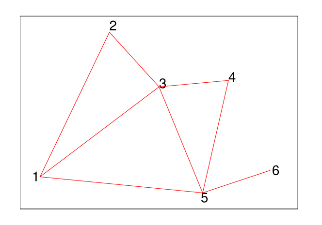
Figure 1: Graph of the six main cities in Mexico numbered from 1 to 6: Guadalajara, Zacatecas, Queretaro, Pachuca, Mexico City, Puebla. The links represent the main roads connecting these cities.

For this particular example, the term $\Delta$ is

$$\epsilon\Delta\equiv\epsilon\left(\begin{array}[]{cccccc}-3&1&1&0&1&0\\ 1&-2&1&0&0&0\\ 1&1&-4&1&1&0\\ 0&0&1&-2&1&0\\ 1&0&1&1&-4&1\\ 0&0&0&0&1&-1\end{array}\right).$$ (11)

Note that the graph Laplacian $\Delta$ is a non-negative symmetric matrix [9]. We use this property below. In physical units the parameter $\epsilon$ is

$$\epsilon=\frac{D}{h^{2}},$$ (12)

where $D$ is a diffusion coefficient and $h$ is a typical distance between cities. The typical time for the diffusion is then

$$t=\frac{1}{\epsilon}=\frac{h^{2}}{D}.$$ (13)

At this time we assumed the same diffusion coefficient (weight) for all the links of the network. If a node is more or less remote from its neighbors than the other nodes, then one could modify the weight accordingly. With this generalization, we would still have a positive symmetric graph Laplacian.

Let $\tau$ be the triangle $\{(s,i)\in[0,1]^{2},~{}~{}s+i\leq 1\}$. We have the following result.

Lemma 2.1

The unit cube $[0,1]^{N}$ is invariant under the evolution of the Zeldovich (10) and Fisher equations in ${\bf R}^{N}$. The product of the triangles $\tau^{N}$ is invariant under the Kermack-McKendrick (2) system with in ${\bf R}^{2N}$.

The lemma follows from Propositions 4.1, 4.4 in section 4 below (these do not use any of the results of section 3). It is also easy to show that the corresponding vector fields at the point inwards at the boundaries.

3 Fixed points of the Zeldovich model

We want to describe a situation where only some nodes are excited; in the epidemic context, it means that some nodes are infected and the rest are susceptible. Only the Zeldovich model (10) has such stable fixed points; these are generalized static “fronts” where some nodes are close to one and the rest close to zero. Therefore, in this section, we concentrate on the fixed points of the Zeldovich model (10). We will clarify the situation for the Fisher model (9) below and show why it is less interesting. For definiteness, throughout this section, we consider the 6 node graph from Fig. 1; it is clear that the results can be extended to an arbitrary finite graph.

The fixed point equation we solve is

$$F(x,\epsilon)=0,\quad x=[x_{1},\ldots,x_{n}]^{T},$$ (14)

where

$$F_{k}(x,\epsilon)=\epsilon(\Delta x)_{k}+f_{k}(x),\quad\hbox{with}$$ (15)

$$f_{k}(x)=\gamma(1-x_{k})x_{k}(x_{k}-a),\quad k=1,\ldots,n,$$ (16)

$\Delta$ is the graph Laplacian of (11), and $0<a<1$, $\gamma=1$. We will examine how the fixed points depend on the coupling parameter $\epsilon\geq 0$.

For $\epsilon=0$, and every partition of the set of nodes into three subsets $S_{0}$, $S_{a}$, $S_{1}$ we have a solution of $F(x,0)=0$ of the form $x_{j}=0$, if $j\in S_{0}$, $x_{j}=a$, if $j\in S_{a}$, $x_{j}=1$, if $j\in S_{1}$. Clearly, these are the only solutions of $F(x,0)=0$. An inspection of the Jacobian reveals that when $S_{a}$ is empty, these solutions are stable. On the other hand if $S_{a}$ is nonempty these solutions are unstable. The number of unstable direction is the number of sites in $S_{a}$. The solutions where $S_{a}$ is empty are generalizations of the fronts that exist for the one dimensional case, they are the main subject of interest of the article.

3.1 Homogeneous fixed points

Let us now consider the case $\epsilon>0$. The homogeneous fixed points can be analyzed for arbitrary $\epsilon$. For that consider the system linearized around the fixed point $x^{*}$

$${v}_{t}=[\epsilon\Delta+Df(x^{*})]v,~{}$$ (17)

where the Jacobian matrix has elements

$$Df(x^{*})=\delta_{k,m}\gamma(2(1+a)x^{*}_{k}-3{x^{*}_{k}}^{2}-a).$$ (18)

When the fixed points are homogeneous, $DN$ has a very simple form, it can be written

$$Df=-\gamma aI,~{}Df=\gamma(a-1)I,~{}Df=\gamma a(1-a)I$$

respectively for $x^{*}=[0,\ldots,0]^{T}~{}x^{*}=[1,\ldots,1]^{T},i^{*}=[a,\ldots,a]^{T}$, where $I$ is the $N\times N$ identity. The matrix $Df$ is then $cI$ for some real constant $c$, and $\sigma(\epsilon\Delta+Df(x^{*}))$ is $\sigma(\epsilon\Delta)+c$. To study the stability it is then convenient to use the basis of orthogonal eigenvectors of the symmetric matrix $\Delta$ [9]

$$\Delta V^{k}=-\omega_{k}^{2}V^{k},$$

where the eigenfrequencies $\omega_{k}$ verify

$$\omega_{1}=0\leq\omega_{2}\leq\dots\leq\omega_{n}.$$

We write

$$i=\alpha_{1}V^{1}+\alpha_{2}V^{2}\dots+\alpha_{n}V^{n}.$$ (19)

Plugging the above expression into (18) we get the evolution of the amplitude

$${\dot{\alpha}_{k}}=-[\epsilon\omega_{k}^{2}+a]{\alpha_{k}}$$ (20)

for the fixed point $x^{*}=[0,\ldots,0]^{T}$. Clearly it is stable for any $\epsilon$. In a similar way we can show that $x^{*}=[1,\ldots,1]^{T}$ is always stable. The fixed point $x^{*}=[a,\ldots,a]^{T}$ is always unstable since we have an eigenvalue $-\epsilon\omega_{1}^{2}+\gamma a(1-a)>0$.

3.2 Non homogeneous fixed points

For the non homogeneous fixed points the analysis is not so simple. Let us first consider the case $\epsilon>0$ but small. The implicit value theorem implies that each solution $x_{0}$ of $F(x,0)=0$ can be continued uniquely, that is, it belongs to a unique smooth one-parameter family of $x(\epsilon)$ satisfying $F(x(\epsilon),\epsilon)=0$, $x(0)=x_{0}$, provided that $|\epsilon|$ is sufficiently small, see e.g. [17]. The solution $x(\epsilon)$ of the local branch passing from $x(0)$ has the same stability as $x(0)$, for $|\epsilon|$ sufficiently small. This follows from the fact that all the solutions $x(0)$ are hyperbolic.

The numerical solutions below were obtained using the minpack implementation of Powell’s hybrid Newton method [16]. We start from $\epsilon=0$, solving (14) using Newton’s method and step in $\epsilon$. After some $\epsilon$, we continue stepping but use the pseudo-arc as a parameter[14] because we anticipate a fold. The linear stability of a solution $x(\epsilon_{0})$ is computed readily by examining the eigenvalues of $D_{1}F(x,\epsilon)$ at $x(\epsilon_{0})$, $\epsilon_{0}$, i.e.

$$(D_{1}F(x,\epsilon))_{n,m}=\epsilon\Delta_{n,m}+\delta_{n,m}\gamma(2(1+a)x_{n}-3x_{n}^{2}-a).$$ (21)

We see numerically that all solutions of $F(x,\epsilon)=0$ with $\epsilon>0$ satisfy $x_{j}\in(0,1)$, forall $j\in\{1,\ldots,6\}$. This is also shown in Corollary 3.3 below. As we increase the value of $\epsilon$ along a branch of solutions continued from an $\epsilon=0$ solution $x_{0}$, the linear stability remains unchanged, until some $\epsilon_{0}$, depending on the branch, where we see a fold. The branch is then continued by decreasing $\epsilon$, until we reach a different solution ${\tilde{x}}(0)$ of the $\epsilon=0$ problem. After the fold the number of stable and stable eigenvalues changes. We observe that when $x(0)$ is stable, the branch changes stability at the fold, and ${\tilde{x}}(0)$ is unstable. For example, setting $a=0.1$, we see that the unstable $\epsilon=0$ solution $[1,1,1,0,0.1,0]^{T}$ is connected to the stable $\epsilon=0$ solution $[1,1,1,0,0,0]^{T}$ by a branch that has a fold at $\epsilon=0.00131035764$. In Fig. 2 we show the value of the component $x_{5}$ at different values of $\epsilon$ of the fixed point. The other components start, and finish at the same values.

A similar behavior was observed for all the examples examined, except the spatially homogeneous solutions $c[1,\ldots,1]^{T}$ with $c=1$, $a$, or $0$. From relation (16) one can see that these exist for all $\epsilon$. Based on our numerical observations we conjecture that all $3^{6}-3$ inhomogeneous fixed points of the $\epsilon=0$ problem (we exclude the spatially homogeneous solutions) belong to branches undergoing a fold bifurcation at some positive value of $\epsilon$, i.e. we have $(3^{6}-3)/2$ branches with folds, connecting pairs of $\epsilon=0$ solutions. This conjecture can be checked numerically by continuing all $\epsilon=0$ fixed points. From the theoretical point of view we can also show that non-spatially homogeneous fixed points cannot exist for arbitrarily large $\epsilon$. We have

Proposition 3.1

There is an $\epsilon_{c}>0$, such that all $(x,\epsilon)$, $x\in I^{N}$, $\epsilon>\epsilon_{c}$ that satisfy $F(x,\epsilon)=0$ are of the form $x=c[1,\ldots,1]^{T}$, with $c=0$, $a$, or $1$.

The proof is given at the end of this section. The dynamical importance of $\epsilon_{c}$ will be discussed further in the next section. The general idea is that for $\epsilon>\epsilon_{c}$ all initial conditions ($\neq a[1,\ldots,1]^{T}$) should go to one of the two fixed points $c[1,\ldots,1]^{T}$, $c=1$, $0$, as $t\rightarrow\infty$.

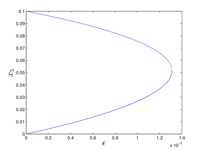
Figure 2: Component $x_{5}$ v.s. $\epsilon$ for a branch connecting the $\epsilon=0$ fixed points $(1,1,1,0,0.1,0)$ and $(1,1,1,0,0,0)$.

An interesting problem is the computation of $\epsilon_{c}$. One idea is to continue all branches starting at $\epsilon=0$ solutions and find the largest value $\epsilon_{0}$ of a fold. This computation would give a lower estimate of $\epsilon_{c}$, since we can not at present rule out the possibility of fixed points not belonging to these branches. Also it is of interest to see whether we can have a family of fixed points $x(\epsilon)$ that are stable for $\epsilon$ arbitrarily close to $\epsilon_{c}$, e.g. a continuous branch having a fold with change of stability at $\epsilon_{c}$. To obtain a first estimation of $\epsilon_{c}$ we have examined numerically all branches starting from stable $\epsilon=0$ solutions for a fixed value of $a$. There are $2^{6}-2$ such branches (we exclude $c[1,\ldots,1]^{T}$, with $c=1$, $0$). These are solutions $x(0)$ with $S_{a}=\emptyset$. In all (non-spatially homogeneous) cases these solutions are connected to an unstable solution ${\tilde{x}}(0)$ of the $\epsilon=0$ problem, with $S_{a}\neq\emptyset$. For $a=0.1$, the largest value of the fold coupling $\epsilon_{0}$ is ${\overline{\epsilon}}_{0}=0.00299835224$, and is observed for the branch connecting the $\epsilon=0$ solutions $[0,0,0,0,0,1]^{T}$ and $[0,0,0,0,0.1,1]^{T}$.

Note that the $\epsilon=0$ solution $[0,0,0,0,0,1]^{T}$ has only one neighbor. This is read from the Laplacian (11). It is reasonable to expect that the solutions that are the last to exist have the least neighbors. We see from (11) that all other $\epsilon=0$ solutions with $|S_{1}|=0$ have more that two neighbors, and it is observed that the corresponding branches undergo folds at smaller values of $\epsilon$. For example the branch starting from $[0,0,0,1,0,0]^{T}$, with two neighbors by (11), undergoes a fold at $\epsilon_{0}=0.00281313677$, while the branch starting from $[0,0,0,0,1,0]^{T}$, with four neighbors, undergoes a fold at $\epsilon_{0}=0.00252927787$. The notion of neighbors can be extended to ($|S_{a}|=0$) $\epsilon=0$ solutions with $|S_{1}|>1$. In such cases we can look for the number of external connections to the set $S_{1}$, i.e. the number of points having distance one from $S_{1}$. We see that more sites in $S_{1}$ generally imply lower $\epsilon_{0}$ in the corresponding branch. For example the branch starting from $[1,1,1,1,1,0]^{T}$, where $S_{1}$ has one external connection, undergoes a fold at $\epsilon_{0}=0.00250694432$. This is lower that the value of the fold value $\epsilon_{0}$ of the branch starting from $[0,0,0,1,0,0]^{T}$ above, with two neighbors but fewer peaks. Comparing the values of $\epsilon_{0}$ for the branches corresponding to $[0,0,0,0,0,1]^{T}$ and $[1,1,1,1,1,0]^{T}$, we also see that complementary $\epsilon=0$ solutions $x(0)$, $x^{\prime}(0)$ (with $|S_{a}|=0$), i.e. ones with $S_{1}(x(0))$, $S_{1}(x^{\prime}(0))$ that are disjoint and whose union is the set of all nodes, generally have corresponding branches with different fold values.

The $\epsilon=0$ solutions not considered in the above enumeration are expected to correspond to branches of solutions that are linearly unstable. Thus, even if we find a static solution such that $\epsilon_{0}>{\overline{\epsilon}}_{0}=0.00299835224$, we expect that for $\epsilon>{\overline{\epsilon}}_{0}$, almost all initial conditions of the time dependant system (10) go to either $c[1,\ldots,1]^{T}$, $c=1$, $0$, as $t\rightarrow\infty$.

To better understand how $\epsilon_{0}$ depends on the type of front and node connectivity, we develop a simple argument that assumes $\epsilon_{0}$ is small, and that all sites except one that we call $n_{c}$ have values $1+O(\epsilon)$, or $O(\epsilon)$, see subsection 3.3 below. This is consistent with what we see numerically, namely that the node that is destabilized first has value approximatelly $a/2$, see e.g. Fig. 2. Other sites have values that are much lower. The argument is as follows. Call $x$ the value of the node $n_{c}$ that will first destabilize. Then the equation at $n_{c}$ for $x$ is

$$\epsilon(N-Kx+O(\epsilon))+x(1-x)(x-a)=0~{},$$

where $N$ is the number of neighbors of $n_{c}$ that are at 1 and $K$ is the connectivity of $n_{c}$. This yields

$$\epsilon={x(1-x)(x-a)\over Kx-N}.$$ (22)

From the continuation study of the static solutions we have seen that for

$$\epsilon=\epsilon_{0},~{}~{}x\approx a/2~{}.$$

Combining this observation with (22) yields the estimate for

$$\epsilon_{0}={a^{2}\over 4}{2-a\over 2N-Ka}.$$ (23)

This estimate is reported in Table 1 below, together with the $\epsilon_{o}$ found numerically. For $a$ relatively small, e.g. for $a=0.1$ used here, we see excellent agreement.

3.3 Asymptotics of the fixed points

In what follows we show some general results on the profile of the fixed points of (10) for $\epsilon>0$, and small. We estimate the decay of the fixed point profiles away from the sites where the solution is near unity; we also see that we can obtain small $\epsilon$ asymptotics for $x(\epsilon)$ at all sites. For instance, we show that the amplitude $x_{n}(\epsilon)$ of the equilibrium at the site $n$ is

$$x_{n}(0)+O(\epsilon^{d_{n}}),$$

where $d_{n}$ is the distance of site $n$ from the analogue of the “interface” of the $\epsilon=0$ configuration, see Lemma 3.6. Roughly speaking, the interface or “front” of an $\epsilon=0$ configuration, defined more precisely below, consists of the sites where the solution jumps from zero to unity. The small $\epsilon$ asymptotic gives us information on the decay of the $x_{n}(\epsilon)$ as we move away form the sites that are near unity. For sites with value near unity it also tells us that are further away from the interface have values that are much closer to unity.

Proposition 3.2 can be also used to compare small $\epsilon$ solutions continued from different $x(0)$, see Corollary 3.5 below.

The proof of Proposition 3.2 is based on small$-\epsilon$ expansions

$$x_{n}(\epsilon)=\sum^{\infty}_{m=0}a_{n,m}\epsilon^{m},$$

valid for all sites $n$. The idea is to insert these expression into (16) and examine the coefficients of the series. We first obtain a less precise, intermediate statement, Lemma 3.6, using induction on the distance from the “interface” between ones and zeros of the $\epsilon=0$ solutions. Proposition 3.2 uses the same strategy, and Lemma 3.6.

The precise statements use the following definitions and notation.

Let $\hbox{nbd}(n)$ denote the sites adjacent to the site $n$. Let $c_{n}=|\hbox{nbd}(n)|$. Let $\hbox{dist}(R,n)$ denote the distance between the set of sites $R$, and a node $n$.

Given a nontrivial solution $x(0)$ of the $\epsilon=0$ equation $F=0$, denote by $S_{1}$, $S_{a}$, $S_{0}$ the sets of indices $n$ where $x_{n}=1$, $a$, $0$ respectively. Also let $S_{A}=S_{1}\cup S_{a}$. Let $I$ be the set of nodes $n\in S_{1}$ having at least one neighbor $j\in S_{a}\cup S_{0}$. The set $I$ plays the role of the “interface” of the configuration.
Then we have:

Proposition 3.2

Let $x(0)$ be a nontrivial solution of equation (14), (16) with $\epsilon=0$, and let $x(\epsilon)$, $\epsilon\in[0,\epsilon_{0}]$ denote the unique branch of solutions of $F=0$, $\epsilon>0$, that continue $x(0)$ for $\epsilon\geq 0$. Consider the sets $S_{1}$, $S_{a}$, $S_{0}$, and $I$ corresponding to $x(0)$ as defined above, with $S_{i}$, $I$ nonempty. Then for $\epsilon>0$ sufficiently small we have that (i) $n\in S_{0}$, $\hbox{dist}(S_{A},n)=m\geq 1$ imply

$$x_{n}(\epsilon)=a_{n,m}\epsilon^{m}+O(\epsilon^{m+1}),\quad\hbox{with}\quad a_{n,m}>0,$$ (24)

and (ii) $n\in S_{1}$, $\hbox{dist}(I,n)=m\geq 0$ imply

$$x_{n}(\epsilon)=1+a_{n,m+1}\epsilon^{m+1}+O(\epsilon^{m+2}),\quad\hbox{with}\quad a_{n,m+1}<0,$$ (25)

An immediate consequence is:

Corollary 3.3

Let $x(0)$ be a nontrivial solution equation (16) with $\epsilon=0$, and let $x(\epsilon)$, $\epsilon\in[0,\epsilon_{0}]$ denote the unique branch of solutions of (16), $\epsilon>0$, that continue $x(0)$ for $\epsilon\geq 0$. Then for $\epsilon>0$ and sufficiently small we have $x_{n}(\epsilon)\in(0,1)$, for all sites $n$.

Proof. For sites $n\in S_{a}$ we have $x_{n}(\epsilon)=a+O(\epsilon)\in(0,1)$ for $\epsilon$ sufficiently small. For other sites the statement follows form Proposition 3.2. $\Box$

Remark 3.4

The above asymptotic is appears to be related to the estimate of $\epsilon_{0}$ in 23, and the assumption that the all sites $n\neq n_{c}$ have values $1+O(\epsilon)$, and $O(\epsilon)$. Indeed most sites $n\neq n_{c}$ are seen to be $O(\epsilon)$ from their $\epsilon=0$ values at $\epsilon_{0}$. Note however that the site $n_{c}$ also has the value $0$ (or $\alpha$) at $\epsilon=0$, and comes near $a/2$ as $\epsilon$ approaches $\epsilon_{0}$. The use of the small$-\epsilon$ asymptotic in justifying 23 is not clear.

Another consequence of Proposition 3.2 is that for $\epsilon>0$ sufficiently small there exist pairs of static solutions $x$, $y$ of the Zeldovich equation satisfying $x_{n}<y_{n}$, $\forall n\in\{1,\ldots,N\}$. The construction is as follows:

Corollary 3.5

Let $x(\epsilon)$, $y(\epsilon)$, $\epsilon$ sufficiently small, be continuations of the $\epsilon=0$ fixed points $x=x(0)$, $y=y(0)$ of the Zeldovich equation satisfying

$$(i)\quad S_{\alpha}(x)=S_{\alpha}(y)=\emptyset,\quad(ii)\quad S_{1}(x)\subset S_{1}(y),$$ (26)

$$(iii)\quad\hbox{dist}(I(x),n)<\hbox{dist}(I(y),n),\quad\forall n\in S_{1}(x)\cup S_{1}(y),$$ (27)

$$(iv)\quad\hbox{dist}(S_{1}(x),n)>\hbox{dist}(S_{1}(y),n),\quad\forall n\in S_{0}(x)\cup S_{0}(y).$$ (28)

Then for all $\epsilon>0$ sufficiently small we have $x_{n}(\epsilon)<y_{n}(\epsilon)$, $\forall n\in\{1,\ldots,N\}$.

Proof. We consider the three cases $n\in S_{0}(x)\cup S_{1}(y)$, $S_{1}(x)\cup S_{1}(y)$, and $S_{0}(x)\cup S_{0}(y)$. By (ii) $S_{1}(x)\cup S_{0}(y)=\emptyset$. For $n\in S_{0}(x)\cup S_{1}(y)$ we have

$$y_{n}(\epsilon)=1-O(\epsilon)>x_{n}(\epsilon)=O(\epsilon),$$

for $\epsilon>0$ small.

For $n\in S_{1}(x)\cup S_{1}(y)$, Proposition 3.2 yields

$$x_{n}(\epsilon)=1-|a_{n,m+1}|\epsilon^{m+1}+O(\epsilon^{m+2}),$$

$$y_{n}(\epsilon)=1-|a_{n,{\tilde{m}}+1}|\epsilon^{{\tilde{m}}+2}+O(\epsilon^{{\tilde{m}}+2}),$$

with $a_{n,m}$, $a_{n,{\tilde{m}}+1}\neq 0$, and

$$m=\hbox{dist}(I(x),n),\quad{\tilde{m}}=\hbox{dist}(I(y),n),\quad{\tilde{m}}>m.$$

Therefore $y_{n}(\epsilon)>x_{n}(\epsilon)$ for $\epsilon>0$ small enough.

For $n\in S_{0}(x)\cup S_{0}(y)$, Proposition 3.2 yields

$$x_{n}(\epsilon)=|a_{n,\mu}|\epsilon^{\mu}+O(\epsilon^{\mu+1}),$$

$$y_{n}(\epsilon)=|a_{n,{\tilde{\mu}}}|\epsilon^{{\tilde{\mu}}}+O(\epsilon^{{\tilde{\mu}}+1}),$$

with $a_{n,\mu}$, $a_{n,{\tilde{\mu}}+1}\neq 0$, and

$$\mu=\hbox{dist}(I(x),n),\quad{\tilde{\mu}}=\hbox{dist}(I(y),n),\quad\mu>{\tilde{\mu}}.$$

Again $y_{n}(\epsilon)>x_{n}(\epsilon)$ for $\epsilon>0$ small enough. $\Box$

The proof of Proposition 3.2 uses the following intermediate result.

Lemma 3.6

Let $x(0)$ be a nontrivial solution equation $F=0$ with $\epsilon=0$, and let $x(\epsilon)$, $\epsilon\in[0,\epsilon_{0}]$ denote the unique branch of solutions of $F=0$, $\epsilon>0$, that continue $x(0)$ for $\epsilon\geq 0$. Consider the sets $S_{1}$, $S_{a}$, $S_{0}$, and $I$ corresponding to $x(0)$ as defined above, with $S_{1}$, $I$ nonempty. Then for $\epsilon>0$ sufficiently small we have that (i) $n\in S_{0}$, $\hbox{dist}(S_{A},n)\geq m\geq 1$ imply

$$x_{n}(\epsilon)=O(\epsilon^{m}),$$ (29)

and (ii) $n\in S_{1}$, $\hbox{dist}(I,n)\geq m\geq 0$ imply

$$x_{n}(\epsilon)=1+O(\epsilon^{m+1}).$$ (30)

Proof. We use the analytic version of the implicit value theorem, which allows us to write $x_{n}(\epsilon)$ as a convergent power series in $\epsilon$, for $\epsilon$ sufficiently near the origin. Thus we write $x_{n}(\epsilon)=\sum^{\infty}_{m=0}a_{n,m}\epsilon^{m}$, for all sites $n$, see e.g. [17]. (Since the network is finite it is sufficient to use the $C^{r}$ version for $r$ sufficiently large.)

We then already have $x_{n}(\epsilon)=O(\epsilon)$, $\forall n\in S_{0}$, and $x_{n}(\epsilon)=1+O(\epsilon)$, $\forall n\in S_{1}$.

To show (i) let $n$ satisfy $\hbox{dist}(S_{A},n)\geq 2$. We have

$$\epsilon(\Delta x)_{n} = \epsilon[-c_{n}(a_{n,1}\epsilon+O(\epsilon^{2}))+\sum_{j\in\hbox{nbd}(n)}x_{j}]$$ (31)

$$= O(\epsilon^{2}),$$

since $j\in\hbox{nbd}(n)$ implies $j\in S_{0}$, hence $x_{j}=O(\epsilon)$.

Also

$$x_{n}(1-x_{n})(a-x_{n})=-aa_{n,1}\epsilon+O(\epsilon^{2}).$$ (32)

By (31), (32), and $F=0$ we must then have $a_{n,1}=0$.

We use induction: suppose that if $\hbox{dist}(S_{A},n)\geq m\geq 2$, then $x_{n}=O(\epsilon^{m})$.

Then for $n$ satisfying $\hbox{dist}(S_{A},n)\geq m+1$ we have

$$\epsilon(\Delta x)_{n} = \epsilon[-c_{n}(a_{n,m}\epsilon^{m}+O(\epsilon^{m+1}))+\sum_{j\in\hbox{nbd}(n)}x_{j}]$$ (33)

$$= O(\epsilon^{m+1}),$$

since $j\in\hbox{nbd(n)}$ implies $\hbox{dist}(S_{A},n)\geq m$, hence $x_{j}=O(\epsilon^{m})$ by the inductive hypothesis. On the other hand

$$x_{n}(1-x_{n})(a-x_{n})=-aa_{n,m}\epsilon^{m}+O(\epsilon^{m+1}).$$ (34)

By (33), (34), and $F=0$ we must then have $a_{n,m}=0$, and therefore $x_{n}=O(\epsilon^{m+1})$, as required.

To see (ii) let $n\in S_{1}$ satisfy $\hbox{dist}(I,n)=1$, so that all $j\in\hbox{nbd}(n)$ satisfy $x_{j}(0)=1$. Also $x_{n}=1+O(\epsilon)$. Then

$$\epsilon(\Delta x)_{n} = \epsilon[-c_{n}(1+a_{n,1}\epsilon+O(\epsilon^{2}))+\sum_{j\in\hbox{nbd}(n)}x_{j}]$$ (35)

$$= \epsilon[-c_{n}-c_{n}a_{n,1}\epsilon+c_{n}+\sum_{j\in\hbox{nbd}(n)}a_{j,1}\epsilon+O(\epsilon^{2})]$$

$$= O(\epsilon^{2}).$$

On the other hand

$$x_{n}(1-x_{n})(a-x_{n})=-(a-1)a_{n,1}\epsilon+O(\epsilon^{2}).$$ (36)

By (35), (36), and $F=0$ we must have $a_{n,1}=0$, and therefore $x_{n}=O(\epsilon^{2})$.

For the inductive step, assume that if $n\in S_{1}$ satisfies $\hbox{dist}(I,n)\geq m$, then $x_{n}=1+O(\epsilon^{m+1})$. Consider then a site $n$ satisfying $\hbox{dist}(I,n)\geq m+1$, then

$$\epsilon(\Delta x)_{n} = \epsilon[-c_{n}(1+a_{n,m+1}\epsilon^{m+1}+O(\epsilon^{m+2}))+\sum_{j\in\hbox{nbd}(n)}x_{j}]$$ (37)

$$= \epsilon[-c_{n}-c_{n}a_{n,m+1}\epsilon^{m+1}+c_{n}+\sum_{j\in\hbox{nbd}(n)}a_{j,m}\epsilon^{m+1}+O(\epsilon^{m+2})]$$

$$= O(\epsilon^{m+2}),$$

using the fact that $j\in\hbox{nbd}(n)$ implies $\hbox{dist}(I,j)\geq m$, hence $x_{j}=1+O(\epsilon^{m+1})$ by the inductive hypothesis. On the other hand

$$x_{n}(1-x_{n})(a-x_{n})=-(a-1)a_{n,m+1}\epsilon^{m+1}+O(\epsilon^{m+2}).$$ (38)

By (37), (38), $F=0$ implies $a_{n,m+1}=0$, and therefore $x_{n}=1+O(\epsilon^{m+2})$, as required. $\Box$

We now prove Proposition 3.2.

Proof. The starting point is again the expression $x_{n}(\epsilon)=\sum^{\infty}_{m=0}a_{n,m}\epsilon^{m}$. To see (i) first consider sites $n$ satisfying $\hbox{dist}(S_{A},n)=1$. Letting $J_{1}$ be the set of sites $j\in\hbox{nbd}(n)\cap S_{A}$, and $J_{2}=\hbox{nbd}(n)\setminus J_{1}$, we have

$$|J_{1}|=|\hbox{nbd}(n)\cap S_{1}|+|\hbox{nbd}(n)\cap S_{a}|>0.$$

Then

$$\epsilon(\Delta x(\epsilon))_{n} = \epsilon[-c_{n}O(\epsilon)+\sum_{j\in J_{1}}x_{j}+\sum_{j\in J_{2}}x_{j}]$$ (39)

$$= (|\hbox{nbd}(n)\cap S_{1}|+|\hbox{nbd}(n)\cap S_{a}|a)\epsilon+O(\epsilon^{2})$$

$$> 0$$

for $\epsilon>0$ sufficiently small. On the other hand

$$x_{n}(1-x_{n})(x_{n}-a)=-a\epsilon a_{n,1}+O(\epsilon^{2}).$$ (40)

By (39), (40), $F=0$, we need $a_{n,1}>0$.

We proceed inductively, assuming that if $n\in S_{0}$ satisfies $\hbox{dist}(S_{A},n)=m\geq 1$, then $x_{n}(\epsilon)=a_{n,m}\epsilon^{m}+O(\epsilon^{m+1})$, with $a_{n,m}>0$. Consider then a site $n$ satisfying $\hbox{dist}(S_{A},n)=m+1$. Let $J_{m}$ be the set of sites $j\in\hbox{nbd}(n)$ satisfying $\hbox{dist}(S_{A},n)=m$. Clearly $|J_{m}|>0$. Also let $J_{m+1}=\hbox{nbd}(n)\setminus J_{m}$. By Lemma 3.6, $x_{n}(\epsilon)=O(\epsilon^{m+1})$. Then

$$\epsilon(\Delta x(\epsilon))_{n} = \epsilon[-c_{n}(a_{n,m+1}\epsilon^{m+1}+O(\epsilon^{m+2}))+\sum_{j\in J_{m}}x_{j}+\sum_{j\in J_{m+1}}x_{j}]$$ (41)

$$= \sum_{j\in J_{m}}a_{j,m}\epsilon^{m+1}+O(\epsilon^{m+2})$$

$$> 0$$

for $\epsilon>0$ small, since $a_{j,m}>0$, $\forall j\in J_{m}$, by the inductive hypothesis. On the other hand

$$x_{n}(1-x_{n})(x_{n}-a)=-aa_{n,m+1}\epsilon^{m+1}+O(\epsilon^{m+2}).$$ (42)

By (41), (42), and $F=0$, we therefore need $a_{n,m+1}>0$.

To see (ii) consider a site $n\in S_{1}\cap I$, so that $\hbox{dist}(I,n)=0$. Then $x_{n}(\epsilon)=1+a_{n,1}\epsilon+O(\epsilon^{2})$, and

$$\epsilon(\Delta x(\epsilon))_{n} = \epsilon[-c_{n}(1+O(\epsilon))+\sum_{j\in\hbox{nbd}(n)\cap S_{1}}x_{j}+\sum_{j\in\hbox{nbd}(n)\cap S_{a}}x_{j}]$$ (43)

$$= \epsilon(-c_{n}+|\hbox{nbd}(n)\cap S_{1}|+|\hbox{nbd}(n)\cap S_{\alpha}|a)+O(\epsilon^{2})].$$

Suppose $\mu=|\hbox{nbd}(n)\cap S_{\alpha}|\geq 1$, then $|\hbox{nbd}(n)\cap S_{1}|\leq c_{n}-\mu$, and (43) yield

$$\epsilon(\Delta x(\epsilon))_{n} \leq \epsilon(-c_{n}+(c_{n}-\mu)+a\mu)+O(\epsilon^{2})$$ (44)

$$= (-1+a)\mu\epsilon+O(\epsilon^{2})$$

$$< 0,$$

for $\epsilon>0$ sufficiently small. If $\mu=0$, $n\in I$ implies $|\hbox{nbd}(n)\cap S_{1}|<c_{n}$, so that (43) implies

$$\epsilon(\Delta x(\epsilon))_{n} \leq \epsilon(-c_{n}+(c_{n}-1)+O(\epsilon^{2})$$ (45)

$$= -\epsilon+O(\epsilon^{2})$$

$$< 0,$$

for $\epsilon>0$ sufficiently small. Combining (44), (45) with

$$x_{n}(1-x_{n})(x_{n}-a)=-a_{n,1}(1-\alpha)\epsilon+O(\epsilon^{2}),$$ (46)

we see that to satisfy $F=0$ with $\epsilon>0$, sufficiently small we must have $-a_{n,1}>0$.

For the inductive step, assume that $n\in S_{1}$, $\hbox{dist}(I,n)=m$ imply $x_{n}(\epsilon)=1+a_{n,m+1}\epsilon^{m+1}+O(\epsilon^{m+2})$ with $a_{n,m+1}<0$. Then let $n\in S_{1}$, $\hbox{dist}(I,n)=m+1$. Let $J_{m}$ be the set of sites $j\in\hbox{nbd}(n)$ satisfying $\hbox{dist}(I,n)=m$, let $J_{m+1}$ be the set of sites $j\in\hbox{nbd}(n)$ satisfying $\hbox{dist}(I,n)\geq m+1$.

By Lemma 3.6 we have $x_{n}(\epsilon)=1+O(\epsilon^{m+2})$. Then

$$\epsilon(\Delta x(\epsilon))_{n} = \epsilon[-c_{n}(1+O(\epsilon^{m+2}))+\sum_{j\in J_{m}}x_{j}+\sum_{j\in J_{m+1}}x_{j}]$$ (47)

$$= \epsilon[-c_{n}+|J_{m}|+\sum_{j\in J_{m}}a_{j,m+1}\epsilon^{m+1}+(c_{n}-|J_{m}|)+O(\epsilon^{m+2})]$$

$$= \sum_{j\in J_{m}}a_{j,m+1}\epsilon^{m+2}+O(\epsilon^{m+3})]$$

$$< 0$$

for $\epsilon>0$ sufficiently small, since $a_{j,m+1}<0$, $\forall j\in J_{m}$ by the inductive hypothesis. On the other hand,

$$x_{n}(1-x_{n})(x_{n}-a)=-(1-a)a_{n,m+2}\epsilon^{m+2}+O(\epsilon^{m+3}).$$ (48)

By (47), (48) to satisfy $F=0$ we must have $-a_{n,m+2}>0$, as required. $\Box$

We now prove Proposition 3.1

Proof. To study large $\epsilon$ solutions of $F(x,\epsilon)=0$ we will equivalently examine $\mu\rightarrow 0^{+}$ solutions ${\tilde{F}}(x,\mu)=0$, where

$${\tilde{F}}_{n}(x,\mu)=(\Delta x)_{n}+\mu f_{n}(x),$$ (49)

$n=1,\ldots,N$.

Then $F(x,\epsilon)=0$, $\epsilon>0$, is equivalent to ${\tilde{F}}(x,\mu)=0$, with $\mu=\epsilon^{-1}$.

Consider a a sequence $\{(x_{n},\epsilon_{n})\}_{n\in{\bf Z}^{+}}\in I^{N}\times{\bf R}^{+}$, satisfying $\epsilon_{n}\rightarrow\infty$, and $F(x_{n},\epsilon_{n})=0$, $\forall n\in{\bf Z}^{+}$. Such sequences clearly exist. Moreover $(x_{n},\mu_{n})$, with $\mu_{n}=(\epsilon_{n})^{-1}$, satisfy ${\tilde{F}}(x_{n},\mu_{n})=0$, $\forall n\in{\bf Z}^{N}$. The sequence of solutions $\{(x_{n},\mu_{n})\}_{n>n_{0}}$ of ${\tilde{F}}=0$ belongs to $I^{N+1}=I^{N}\times[0,1]$ for some $n_{0}>0$, and by the compactness of $I^{N+1}$ has a convergent subsequence in $I^{N+1}$, denoted again as $\{(x_{n},\mu_{n})\}_{n\in{\bf Z}^{+}}$. Let $(x_{*},\mu_{*})$ be the limit of this subsequence. By the assumption $\epsilon_{n}\rightarrow\infty$, we have that $\mu_{*}=0$. Also, ${\tilde{F}}:{\bf R}^{N+1}\rightarrow{\bf R}^{N+1}$ is continuous and therefore ${\tilde{F}}(x_{n},\mu_{n})\rightarrow{\tilde{F}}(x_{*},0)$ as $(x_{n},\mu_{n})\rightarrow(x_{*},0)$. Therefore ${\tilde{F}}(x_{*},0)=0$. Since ${\tilde{F}}(x,0)=\Delta x$ we have $x_{*}\in V\cap I^{N}$, where $V=\{c[1,\ldots,1]^{T}\in{\bf R}^{N}:c\in{\bf R}\}$, i.e. the kernel of $\Delta$.

We show that $x_{*}$ can only be one of the $c[1,\ldots,1]^{T}$, with $c=0$, $a$, or $1$. Let $P$ the orthogonal projection of ${\bf R}^{N}$ onto $V$. Also let $W=I-P$, where $I$ the identity in ${\bf R}^{N}$. We apply $P$ and $I-P$ to ${\tilde{F}}=0$, and write $x=v+w$, with $v\in V$, $w\in W$. This decomposition is unique. Using the facts that $\Delta$ and $P$ commute, and that $\Delta v=0$, ${\tilde{F}}=0$ becomes

$$Pf(v+w)=0,$$ (50)

$$\Delta w+\mu(I-P)f(v+w)=0.$$ (51)

Fix any $v\in V\cap I^{N}$. We use the implicit function theorem to continue the solution $(w,\mu)=(0,0)$ of (51) to a solution with $\mu\neq 0$. Then for $|\mu|$ sufficiently small there exists a one-parameter family of solutions $(w,\mu)=(h(\mu;v),\mu)$ of (51), where $h(\cdot;v)$ is continuous in $\mu$, with $h(\mu;v)=O(\mu)$ as $\mu\rightarrow 0$ (uniformly in $v$). The implicit function theorem also implies that these solutions are the only solutions of (51) in a sufficiently small neighborhood of $(w,\mu)=(0,0)$ in $W\times{\bf R}$. Similar considerations show that the function $h$ is continuous in $v$, $\forall v\in v\in V\cap I^{N}$.

Thus all solutions of ${\tilde{F}}(x,\mu)$, with $x=v+w$, $v\in V$, $w\in W$, and $w\rightarrow 0$, $\mu\rightarrow 0$, must be of the form $x=v+h(\mu,v)$, with $v$ a solution of

$$g(v,\mu)=Pf(v+h(\mu;v))=0,$$ (52)

by (50).

Suppose that we have a sequence of solutions $\{(v_{n},\mu_{n})\}_{n\in{\bf Z}^{+}}$ of $g(v,\mu)=0$ with $v\in V\cap I^{N}$, and $\mu_{n}\rightarrow 0$. By compactness this sequence has a convergent subsequence. Denote its limit by $(v_{*},0)$. By the continuity of $h$, and therefore of $g$, $v_{*}$ must satisfy $g(v_{*},0)=Pf(v_{*})=0$, hence $v_{*}=v_{r}=c_{r}[1,\ldots,1]^{T}$, $r=1,2,3$ with $c_{1}=0$, $c_{2}=a$, $c_{3}=1$. Applying the implicit function theorem again we check that each of the solutions $v_{r}$, $r=1,2,3$, of $g(v,0)=0$ is continued to a unique branch of solutions of $g(v,\mu)=0$, with $(v,\mu)$. Each of these three branches contains all possible solutions of $g=0$ sufficiently near the respective $(v_{r},0)$, $r=1,2,3$. By uniqueness these three local branches are subsets of the three trivial branches $(v_{r},\mu)$, $r=1,2,3$, $\mu>0$, of solutions of ${\tilde{F}}=0$. $\Box$

4 Comparison results for front propagation models

We now consider the time dependant solutions of the Zeldovich equation (10), and establish qualitative comparison (or monotonicity) results for different solutions of the Zeldovich model, see Proposition 4.1. An application is Corolary 4.2, a stability statement for some of the static solutions discussed in Corolary 3.5 of the previous section. Another goal is to compare the Zeldovich model with the original Kermack-McKendrick system, and the intermediate Fisher system. We show that the Fisher model describes a faster propagation of the epidemic than both the Zeldovich and Kermack-McKendrick models, see Propositions 4.3, 4.4 respectively. In the next section we show some numerical examples.

The comparison statements below use a notion of “partial order” between configurations. In particular $u<n$ (respectively $u\leq v$), with $u$, $v\in[0,1]^{N}$, will mean $u_{n}<v_{n}$ (respectively $u_{n}\leq v_{n}$), $\forall n\in\{1,\ldots,N\}$. We also let ${\bf 0}=[0,\ldots,0]^{T}$, ${\bf 1}=[1,\ldots,1]^{T}\in[0,1]^{N}$. A “larger” configuration thus describes a state where the epidemic is more advanced at all sites.

Proposition 4.1

Let $T>0$, $x$, $y:[0,T]\rightarrow[0,1]^{N}$ be two solutions of (either) the Zeldovich (10) (or the Fisher (9)) equation, with initial conditions satisfying ${\bf 0}<x(0)<y(0)\leq{\bf 1}$. Then $x(t)<y(t)$, $\forall t\in[0,T]$.

Since both vectors ${\bf 0}$, ${\bf 1}$ are static solutions of the Zeldovich and Fisher equations, Lemma 2.1 is a special case of Proposition 4.1.

Corollary 4.2

Let $T>0$. Let $x$, $y\in[0,1]^{N}$ be two static solutions of the Zeldovich equation satisfying $x<y$, and let $u:[0,T]\rightarrow[0,1]^{N}$ be a solution of the Zeldovich equation with initial condition $u(0)$ satisfying $x<u(0)<y$. Then $x<u(t)<y$, $\forall t\in[0,T]$.

The existence of pairs of static solutions of the Zeldovich equation satisfying $x<y$, is shown in the previous section, in Corollary 3.5.

We now compare solutions of the Fisher and Zeldovich equations.

Proposition 4.3

Let $T>0$. Let $x_{F}$, $x_{Z}:[0,T]\rightarrow[0,T]^{N}$ be solutions of the Fisher (9), and Zeldovich (10) equations respectively, with corresponding initial conditions satisfying ${\bf 0}<x_{Z}(0)\leq x_{F}(0)\leq{\bf 1}$. Then $x_{Z}(t)\leq x_{F}(t)$, $\forall t\in(0,T]$.

Proposition 4.4

Let $T>0$. Let $x_{F}:[0,T]\rightarrow[0,1]^{N}$ be a solution of the Fisher equation (9), and let $(s,i):[0,T]\rightarrow\tau^{N}$ satisfy the Kendrick-McKormack system (2). Suppose also that the corresponding initial conditions satisfy $i(0)<x_{F}(0)$. Then $i(t)\leq x_{F}(t)$, $\forall t\in[0,T]$.

The above comparison statements follow from analogous statements for discrete time approximations of the solutions of the three equations. The approximations we use are obtained by the first-order explicit Euler method.

Consider a general ODE ${\dot{z}}=F(z)$ in ${\bf R}^{K}$ with initial condition $z(0)$, and the corresponding solution $z$ in the interval $[0,T]$. Fix a positive integer $M>1$, and let $\Delta t=T/M$. Let $z^{M}$ be an array of $M+1$ vectors $z^{M}(m\Delta t)\in{\bf R}^{K}$, $m\in\{0,\ldots,M\}$, defined iteratively by $z^{M}(0)=z(0)$,

$$z^{M}((m+1)\Delta t)=z^{M}(m\Delta t)+F(z^{M}(m\Delta t))\Delta t,\quad m\in{0,\ldots,M}.$$ (53)

(The dependence of $\Delta t$ on $M$ is not explicit in this notation.) Thus $z^{M}$ is the numerical trajectory obtained by the first order, explicit Euler method with constant time-step ${\Delta t}={T/M}$ over an interval $[0,T]$. We recall a standard convergence result for the Euler method (see e.g. [12]):

Lemma 4.5

Consider the ODE ${\dot{z}}=F(z)$ in ${\bf R}^{K}$ with initial condition $z(0)$, and assume that the solution $z(t)$, $t\in[0,T]$, exists and is unique. Assume also that $F$ is $C^{1}$ in ${\bf R}^{K}$. For every integer $M>1$ let $z^{M}$ be as in (53) with fixed time-step ${\Delta t}={T/M}$ over the interval $[0,T]$. Then

$$\lim_{M\rightarrow\infty}\max_{m\in\{0,\ldots,M\}}||z(m{\Delta t})-z^{M}(m{\Delta t})||=0,$$ (54)

where $||\cdot||$ denotes the norm in ${\bf R}^{K}$.

In the following lemma we compare two Euler approximates of either the Zeldovich or the Fisher equations. We see that they preserve the order of the initial conditions.

Lemma 4.6

Let $T>0$, and let $M>1$ be an integer. Let $x^{M}$, $y^{M}$ be the Euler approximations with time-step ${\Delta t}=T/M$ over the interval $[0,T]$ of two trajectories of either the Zeldovich (10) or the Fisher (9) equations. Assume that $x^{M}(0)<y^{M}(0)$, with $x^{M}(0)$, $y^{M}(0)$ in $[0,1]^{N}$. Then $x^{M}(m{\Delta t})<y^{M}(m{\Delta t})$, $\forall m\in\{1,\ldots,M\}$, provided $M$ is sufficiently large.

The lemma also implies that the Euler approximations of the Zeldovich and Fisher equations with initial conditions in $[0,1]^{N}$ stay in $[0,1]^{N}$, provided the time-step is small enough.

The proof below shows that this step size does not depend on the initial conditions, it only depends on $\Delta$, i.e. the graph, and the functions

$$f_{F}(x)=(1-x)x,\quad f_{Z}(x)=(1-x)x(x-\alpha)$$ (55)

in the equations. The same comment applies to Lemma 4.8.

Proof. Consider the first step of the iteration for the Zeldovich equation, starting with two initial conditions $x^{M}(0)<y^{M}(0)$ in $[0,1]^{N}$.

We have

$$y^{M}(\Delta t)-x^{M}(\Delta t) = y^{M}(0)-x^{M}(0)+$$

$$\Delta t[\epsilon\Delta(y^{M}(0)-x^{M}(0))+f_{Z}(y^{M}(0))-f_{Z}(x^{M}(0))].$$

Examining the components of the $y^{M}(\Delta t)$, $x^{M}(\Delta t)$ we have that for every $k\in\{1,\ldots,N\}$,

$$y_{k}^{M}(\Delta t)-x_{k}^{M}(\Delta t)\geq[1+\Delta t(-\epsilon n_{k}+f_{Z}^{\prime}({\tilde{x}}_{k}))](y_{k}^{M}(0)-x_{k}^{M}(0)),$$ (56)

where ${\tilde{x}}_{k}\in[0,1]$, and $-n_{k}=\Delta_{k,k}$.

To maintain the $y_{k}^{M}(\Delta t)-x_{k}^{M}(\Delta t)$ positive it suffices that

$$1+\Delta t(-\epsilon n_{max}+\min_{x\in[0,1]}f_{Z}^{\prime}(x)>0,$$ (57)

with $n_{max}=\max_{k\in\{1,\ldots,N\}}n_{k}$. This can be achieved for $M$ sufficiently large, and independent of $y^{M}(0)$, $x^{M}(0)$.

Applying this argument to the case where either $x^{M}(0)={\bf 0}$, or $y^{M}(0)={\bf 1}$, both static solutions of the Zeldovich equation, we then have ${\bf 0}\leq x^{M}(\Delta t)<y^{M}(\Delta t)<{\bf 1}$, which also implies $x^{M}(0)$, $y^{M}(0)\in[0,1]^{N}$. We can iterate the argument for all remaining steps, with the same step size $T/M$. The Fisher case is treated similarly. $\Box$

Similarly we compare Euler approximates of the Zeldovich and Fisher equations. We see that the Fisher approximations propagate faster. The proof also shows that $(s(t),i(t))$ remains in $\tau^{N}$ for all times.

Lemma 4.7

Let $T>0$, and let $M>1$ be an integer. Let $x_{Z}^{M}$, $x_{F}^{M}$ be the Euler approximations with time-step ${\Delta t}=T/M$ over the interval $[0,T]$ of the Zeldovich (10) and Fisher (9) equations respectively. Assume that $x_{Z}^{M}(0)\leq x_{F}^{M}(0)$, with $x_{Z}^{M}(0)$, $x_{F}^{M}(0)$ in $[0,1]^{N}$. Then $x_{Z}^{M}(m{\Delta t})<x^{F}(m{\Delta t})$, $\forall m\in\{1,\ldots,M\}$, provided $M$ is sufficiently large.

Proof. The argument is similar to the one used for Lemma 4.6 above and some details are omitted. Consider the first step of the iteration for the Zeldovich and Fisher equations, starting with respective initial conditions $x_{Z}^{M}(0)<x_{F}^{M}(0)$ in $[0,1]^{N}$, and let $f_{Z}$, $f_{F}$ denote the Zeldovich and Fisher nonlinearities respectively. We have

$$x_{F}^{M}(\Delta t)-x_{Z}^{M}(\Delta t) = x_{F}^{M}(0)-x_{Z}^{M}(0)+$$

$$\Delta t[\epsilon\Delta(x_{F}^{M}(0)-x_{Z}^{M}(0))+f_{F}(x_{F}^{M}(0))-f_{Z}(x_{Z}^{M}(0))].$$

From

$$f_{F}(x_{F}^{M}(0))-f_{Z}(x_{Z}^{M}(0)) = [f_{F}(x_{F}^{M}(0))-f_{F}(x_{Z}^{M}(0)]+$$ (58)

$$[f_{F}(x_{Z}^{M}(0))-f_{Z}(x_{Z}^{M}(0))],$$

and

$$(1-x)x\geq(1-x)x(x-\alpha),\quad\alpha\in(0,1),\forall x\in[0,1],$$

the second expression in (58) is a positive vector. Collecting the analogues of the (56) for the components of $x_{F}^{M}(\Delta t)-x_{Z}^{M}(\Delta t)$ we then have

$$x_{F}^{M}(\Delta t)-x_{Z}^{M}(\Delta t)\geq[1+\Delta t(-\epsilon n_{max}+\min_{{x}\in[0,1]}f_{F}^{\prime}(x))](x_{F}^{M}(0)-x_{Z}^{M}(0)).$$

We can then take $M$ sufficiently large and independent of the inital conditions so that ${\bf 0}\leq x_{F}^{M}(\Delta t)<x_{Z}^{M}(\Delta t)\leq{\bf 1}$, and repeat the argument for all steps. $\Box$

Lemma 4.8

Let $T>0$, and let $M>1$ be an integer. Let $x^{M}$, and $(s^{M},i^{M})$ be the Euler approximations with time-step ${\Delta t}=T/M$ over the interval $[0,T]$ of the Fisher (9) and Kendrick-McKormack (2) equations respectively. Assume that $i^{M}(0)\leq x^{M}(0)$, with $x^{M}(0)$ in $[0,1]^{N}$, $(s^{M}(0),i^{M}(0))\in\tau^{N}$. Then $i^{M}(m{\Delta t})<x^{M}(m{\Delta t})$, $\forall m\in\{1,\ldots,M\}$, provided $M$ is sufficiently large. For such $M$ we also have $(s^{M}(m{\Delta t}),i^{M}(m{\Delta t}))\in\tau^{N}$, $\forall m\in\{1,\ldots,M\}$.

Proof. The argument is similar to the one used for Lemmas 4.6, and some details are omitted. Consider the first step of the iteration for the Kendrick-McKormack and Fisher equations, starting with respective initial conditions $x_{F}^{M}(0)$ in $[0,1]^{N}$, $(s^{M}(0),i^{M}(0))\in\tau^{N}$. We have at each site $k$

$$x_{k}^{M}(\Delta t)-i_{k}^{M}(\Delta t) = x_{k}^{M}(0)-i_{k}^{M}(0)+$$ (59)

$$\Delta t[\epsilon(\Delta(x^{M}(0)-i^{M}(0)))_{k}+$$

$$x_{k}^{M}(0)(1-x_{k}^{M}(0))-i_{k}(0)s_{k}(0)+\gamma i_{k}^{M}(0)].\$$

By $s^{M}_{n}(0)+i^{M}_{n}(0)\leq 1$, we therefore have

$$x_{k}^{M}(0)(1-x_{k}^{M}(0))-i_{k}(0)s_{k}(0) \geq x_{k}^{M}(0)(1-x_{k}^{M}(0))-i_{k}(0)(1-i_{k}^{M}(0))+$$ (60)

$$f_{F}^{\prime}({\tilde{x}}_{k})(x_{k}^{M}(0)-i_{k}^{M}(0))$$

for ${\tilde{x}}_{k}$ in $[i_{k}^{M}(0),x_{k}^{M}(0)]\subset[0,1]$. Then we have

$$i^{M}(\Delta t)-x^{M}(\Delta t)\geq[1+\Delta t(-\epsilon n_{max}+\min_{{x}\in[0,1]}f_{F}^{\prime}(x))](x^{M}(0)-i^{M}(0)),$$ (61)

and therefore $i^{M}({\Delta t})<x^{M}({\Delta t})$ for $M$ sufficiently large and independent of the initial conditions.

A similar argument is used to show that $s^{M}(\Delta t)$, $i^{M}(\Delta t)>0$ for $M$ sufficiently large and independent of the initial conditions, and we omit the details.

By Lemma 4.6 similarly have $x^{M}(\Delta t)\in[0,1]^{N}$ for $M$ sufficiently large and independent of the initial conditions. Finally adding the Euler formulas for $s^{M}({\Delta t})$, $i^{M}({\Delta t})$, and using $\Delta{\bf 1}=0$, we have

$${\bf 1}-(s^{M}({\Delta t})+i^{M}({\Delta t})) = {\bf 1}-(s^{M}(0)+i^{M}(0)+$$ (62)

$${\Delta t}[\epsilon({\bf 1}-(s^{M}(0)+i^{M}(0))+\gamma i^{M}(0)]$$

$$\geq (1-{\Delta t}\epsilon d_{max})[{\bf 1}-(s^{M}(0)+i^{M}(0)],$$

which is positive for $M$ sufficiently large and independent of the initial conditions. We can then iterate the argument for the remaining steps. $\Box$

The fact that the convergence of the approximate solutions $x^{M}$ of the Euler method to the trajectory $x$ in Lemma 54 preserves the partial order follows from the following.

Let $\{g^{M}\}=\{g_{M}\}^{\infty}_{M=1}$, denote a sequence of arrays (of increasing size $M+1$) $g^{M}=(g^{M}_{0},\ldots,g^{M}_{M})$ of vectors $g_{m}^{M}\in{\bf R}^{K}$, $m=1,\ldots,M$. Let $\{g^{M}\}\rightarrow g$ denote that

$$\lim_{M\rightarrow\infty}\max_{m\in\{0,\ldots,M\}}||g^{M}_{m}-g(m({T/M}))||=0,$$ (63)

where $g:[0,T]\rightarrow{\bf R}^{K}$, and $||\cdot||$ is the norm in ${\bf R}^{K}$.

Lemma 4.9

Consider sequences $\{g^{M}\}$, $\{h^{M}\}$ as above satisfying that for all $M$ sufficiently large we have that $g^{M}_{m}<h^{M}_{m}$, $\forall m\in\{0,\ldots,M\}$. Suppose also that there exist continuous functions $g$, $h:[0,T]\rightarrow{\bf R}^{K}$ for which $\{g^{M}\}\rightarrow g$, and $\{h^{M}\}\rightarrow h$ respectively. Then $g(t)\leq h(t)$, $\forall t\in[0,T]$.

Proof. The statement follows from continuity of $h-g$ in $[0,T]$, since it is easy to see that $h(t_{0})-g(t_{0})>0$ for some $t_{0}\in(0,T]$ and the convergence leads to a contradiction. $\Box$

We now prove Proposition 4.1.

Proof. Combining the comparison of approximate solutions produced by the Euler method Lemma 4.6, with the approximation Lemmas 4.5, 4.9 we have that $x(0)<y(0)$ implies $x(t)\leq y(t)$, $\forall t\in[0,T]$. To show the strict inequality we use the fact that the evolution can be also defined uniquely also backwards in time. Thus $x(t)\leq y(t)$, for some $t\in(0,T]$ leads to a contradiction. $\Box$

Propositions 4.3, 4.4 follow in the same way, but we can not apply the backwards evolution argument, and do not have strict inequality.

5 Numerical results on front propagation

In the first part of this section we solve numerically the Zeldovich system (10) for initial conditions that are near the computed static solutions. We confirm the results of Section 3 on thresholds, and examine the evolution of the front-like initial conditions for couplings that are above the threshold. In the second part we verify some of the predictions of the comparison results of Section 4. One main observation is that the propagation of the Fisher, and Kermack-McKendrick models is much faster than the ones seen in the Zeldovich models. A third part examines the propagation of Zeldovich fronts for larger values of the local excitation threshold $a$. We can then observe very rapid front propagation. In all simulations below we use the variable step 5-6 dopri5 solver of Hairer and Norsett [11] in double precision with a relative tolerance of $10^{-10}$.

5.1 Time evolution of the Zeldovich fronts

Branches of static solutions $x(\epsilon)$ are labeled by the corresponding $\epsilon\rightarrow 0$ limit $x(0)$, obtained by decreasing $\epsilon$. The value of $\epsilon$ at the fold is $\epsilon_{0}(x(0))$ (or simply $\epsilon_{0}$ when the branch in question is clear). In addition to the numerical and theoretical $\epsilon_{0}$ values from Section 3, we here obtain a third estimate of $\epsilon_{0}$ by integrating (10) starting with $\epsilon<\epsilon_{0}$ and increasing $\epsilon$ slowly on each run. The typical behavior is the following. For small $\epsilon$ we always find a static solution. As $\epsilon$ is increased past a threshold $\epsilon_{0}$, the solution destabilizes and gives rise to the homogeneous flat state $[1,\dots,1]$. This estimated $\epsilon_{0}$ is between the largest $\epsilon$ leading to convergence to a similar static front, and the smallest $\epsilon_{0}$ leading to a trajectory that diverges from the front. The three estimates of $\epsilon_{0}$ are given in Table 1 for some examples, and confirm the results expected from Section 3.

We now present some examples of the evolution slightly above the $\epsilon_{0}$ for different configurations. We examine how the connectivity of a node influences the destabilization of a front centered at that node.

In the first example we consider the evolution from an initial condition near a static front localized at node 6 which (with connectivity 1). The front belongs to the branch of $[0,0,0,0,0,1]^{T}$, which is expected to be last to be destabilized. We use $\epsilon=3.0~{}10^{-3}$, slightly above the computed threshold $\epsilon_{0}=2.998~{}10^{-3}$, and the initial condition

$$[1.536~{}10^{-3},8.680~{}10^{-5},1.537~{}10^{-3},1.578~{}10^{-3},5.350~{}10^{-2},0.997]^{T}.$$ (64)

Notice how it decays very rapidly from the node 5 to the nodes 1 and 4 then node 3. The evolution is shown in Fig. 3, we see that the wave goes successively from 5 ,4 , 3 ,1 and 2.

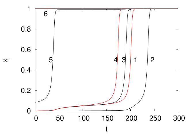
Figure 3: Time evolution of the different nodes for an initial front solution centered on node 6, of connectivity 1, with $\epsilon=3.0~{}10^{-3}$ and the initial condition 64.

In the second example we consider an initial condition near the static solutions of the branch $[0,1,0,0,0,0]^{T}$. We use $\epsilon=2.6875~{}10^{-3}$, which is slightly above computed $\epsilon_{0}=2.547~{}10^{-3}$ for the branch, and the initial condition

$$[5.088~{}10^{-2},0.994,4.298~{}10^{-2},1.165~{}10^{-3},2.35~{}10^{-3},6.132~{}10^{-5}].$$ (65)

The value $x_{1}=5.088~{}10^{-2}$ is very close to $a/2$ which is the value observed by the continuation method for $\epsilon=\epsilon_{c}$. The evolution is shown in Fig. 4. The solution destabilizes following the fixed point so $x_{1}$ and $x_{3}$ remain close to $a/2$ for a long time before going to 1. We see that the wave follows the connectivity as it propagates from node 1 (3) to node 3 (4). Then node 5 (4) destabilizes and finally node 4. Node 6 is just destabilizing for $t=900$. There are then different time scales in the dynamics depending on the connectivity.

We also note that $\epsilon$ is greater than the threshold $\epsilon_{0}=2.5~{}10^{-3}$ for the branch $[1,1,1,1,1,0]^{T}$ (see Section 3), this means that the front will not stop at node 5, it will also destabilize node 6.

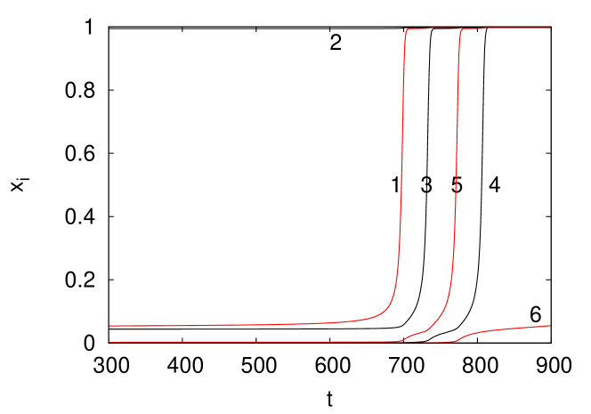
Figure 4: Time evolution of the different nodes for an initial front solution centered on node 2, of connectivity 2, $\epsilon=2.6875~{}10^{-3}$, initial condition in 65.

We now consider an initial condition centered on node 3, near static solutions of the branch $[0,0,1,0,0,0]^{T}$. We use $\epsilon=2.54~{}10^{-3}$, which is slightly above the computed threshold $\epsilon_{0}=2.528~{}10^{-3}$ for the branch, and the initial condition

$$[4.946~{}10^{-2},5.404~{}10^{-2},0.989,4.785~{}10^{-2},4.206~{}10^{-2},1.05410^{-3}].$$ (66)

The evolution given in Fig. 5 shows that the front centered on node 3 of connectivity 4 destabilizes in the same way as the one centered on node 2 except that now nodes 2,1,5 and 4 have values around $a/2$ for a long time. Node 6 will destabilize after a long time. As in the previous example $\epsilon$ is greater than the threshold $\epsilon_{0}=2.5~{}10^{-3}$ for the branch $[1,1,1,1,1,0]^{T}$.

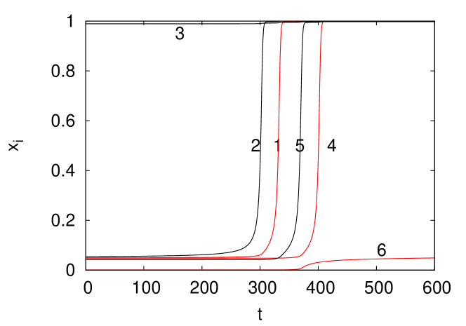
Figure 5: Time evolution of the different nodes for an initial front solution centered on node 3, of connectivity 4, $\epsilon=2.54~{}10^{-3}$, initial condition in 66.

We now consider initial conditions near static solutions of the branch $[1,1,1,0,0,0]^{T}$, see Fig. 6. We use $\epsilon=1.32~{}10^{-3}$, slighly above the critical $\epsilon_{0}=1.3103~{}10^{-3}$ (see Section 4), and the intial condition

$$[0.999,0.99999,0.997,1.610~{}10^{-2},4.980~{}10^{-2},6.485~{}10^{-4}]^{T}$$ (67)

The evolution is shown in Fig. 6. Node 5 is the first to destabilize, followed by node 4. We also see that node 6 remains at its level because $\epsilon$ is smaller than the threshold $\epsilon_{0}$ for the static front of the type $[1,1,1,1,1,0]^{T}$.

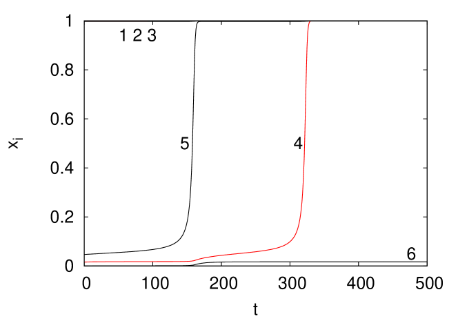
Figure 6: Time evolution of the different nodes for an initial front solution of the type $[1,1,1,0,0,0]^{T}$, with $\epsilon=1.32~{}10^{-3}$ and the initial condition 67.

One can estimate the time for $x_{5}$ to grow, using the normal form displayed in Fig. 2 as a function of $\delta=\epsilon-\epsilon_{c}$. It gives

$${\dot{x}_{5}}=x_{5}^{2}+\delta,$$

so that

$$x_{5}(t)=\sqrt{\delta}\tan(\sqrt{\delta}t),$$ (68)

which grows as $1/\sqrt{\delta}$ We have

$$\epsilon_{c}=1.310^{-3},~{}\epsilon=1.410^{-3},\delta=10^{-4},~{}1/\sqrt{\delta}=100.$$

From Fig. 6 one sees that the typical time of destabilization of $x_{5}$ is about 100 so the estimate is correct.

These results confirm that generalized static fronts exist for small $\epsilon$ and disappear for $\epsilon>\epsilon_{c}$; they are summarized in Table 1.

connectivity	node	branch	$\epsilon_{0}$	$\epsilon_{0}$	expression (23)
			from time evolution	continuation
1	6	$(000001)$	$3.0~{}10^{-3}$	$2.998~{}10^{-3}$	$2.97~{}10^{-3}$
2	2	$(010000)$	$2.7~{}10^{-3}$	X	$2.7910^{-3}$
4	3	$(001000)$	$2.54~{}10^{-3}$	X	$2.6310^{-3}$
2	1 2 3	$(111000)$	$1.31~{}10^{-3}$	$1.310~{}10^{-3}$	$1.32~{}10^{-3}$

Table 1: Critical $\epsilon$ for the ”generalized front” to destabilize for different initial conditions.

The above examples also suggest a qualitative picture of the propagation of fronts, where one can use the analytical expresion (23) for $\epsilon_{0}$ to guess the order in which the differerent nodes are excited. It appears that given a configuration of excited sites, the next site is the one in the neighborhood of the configuration that has the largest number of connections with the configuration connections. In the case where we have more than one such sites, the one that has the fewest connections, see e.g. the example of Fig. 3. This rule is consistent with the calculation of the smallest $\epsilon_{0}$ values from (23) among the possible $n_{c}$ in the vicinity of a configuration. This rule does not include all posibilities, but it points to a possible connection between the $\epsilon_{0}$ for the various branches, and the propagation of the front. An estimation of $\delta=\epsilon-\epsilon_{0}$ leads to an approximate time for the site $n_{c}$ to be excited, using (68).

5.2 Comparison between different solutions and front propagation models

To illustrate the comparison of two initial conditions under the Zeldovich evolutions, we show solutions from initial conditions $[1,1,1,0,0,0]^{T}$ and $[1,1,0,0,0,0]^{T}$ respectively. We use $\epsilon=1.4~{}10^{-3}$. The time evolution is indicated Fig. 7 where the nodes 4 and 5 are shown. The trajectories increase faster for the first initial condition than for the second.

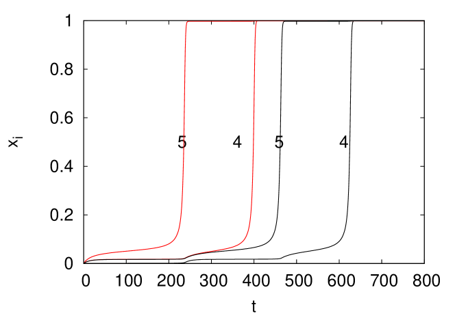
Figure 7: Time evolution of nodes 4 and 5 for the initial fronts $[1,1,1,0,0,0]^{T}$ in continuous line (red online) and $[1,1,0,0,0,0]^{T}$ in dashed line.

To illustrate the comparison between trajectories of the Fisher and Zeldovich equations we use the initial condition $[1,1,0,0,0,0]^{T}$, with $\epsilon=1.4~{}10^{-3}$. It is presented in Fig. 8. Note that the scale in time is much shorter than in Fig. 7 , here for $t=20$ the front has invaded the graph. Therefore the Fisher solution will always be larger than the Zeldovich one. Also the profile is different since there are no fixed points other than the flat 1 homogeneous state.

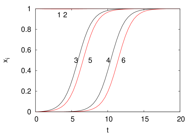
Figure 8: Time evolution of the initial front $[1,1,0,0,0,0]^{T}$.

We also consider the evolution of the Kermack-McKendrick model (2). When the decay term $\beta$ for the infected component $i$ is zero, the evolution of $i$ is identical to the one of the Fisher model (9). This is because (2) conserves $s+i$. For example taking as initial condition

$$s=[0,0,1,1,1,1]^{T},\quad i=[1,1,0,0,0,0]^{T}$$

yields exactly the same dynamics for $i$ as the one of Fig. 8. On the other hand, if we choose $s+i<1$ and still the same initial $i$, then the trajectories of (2) are below the ones of (9). Nevertheless the characteristic time for the orbits of (2) to reach saturation is the same as for (9). When $\beta>0$ is small, the infected component reaches a maximum in this characteristic time and then decays over a time scale $1/\beta$ Fig. 9 shows the evolution of the infected component for $\beta=0.01$ and $\epsilon=1.35~{}10^{-3}$ To see propagation on the network, $\beta$ should be smaller than the diffusion time $1/\epsilon$.

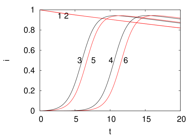
Figure 9: Time evolution of the infected component $i$ for the initial front $s=[0,0,1,1,1,1]^{T},~{}i=[1,1,0,0,0,0]^{T}$ for the Kermack-Mackendrick model (2) with $\beta=0.01$.

The comparisons between the Zeldovich models on the one hand, and the Fisher, and the Kermack-McKendrick models show that the later two lead to a much faster propagation. This makes the comparison between the Fisher, and Kermack-McKendrick models a more interesting result.

The examples above suggest also that the order in which the different nodes become excited in the three models is the same. This order seems to depend only on the geometry of the graph. It may be possible to use different (possibly branch or site dependent) parameters $\epsilon$, $\gamma$, and $a$ for the Zeldovich and Fisher systems to make the propagation speeds comparable.

5.3 Influence of the parameter $a$

To conclude this numerical section, we consider how the fixed points of the Zeldovich equation and its dynamical solutions depend on the parameter $a$. To illustrate how $a$ changes the fixed point and it’s subsequent destabilization, we consider the front centered on node 6 of the type $[000001]^{T}$. For $a=0.3$ and $\epsilon=1.25~{}10^{-3}$ we obtain the static front

$$[0.104,5.477~{}10^{-2},0.107,0.124,0.295,0.852]^{T}.$$ (69)

Compared to the one for $a=0.1$ (64), this front is much broader. Here we see that $x_{5}\approx aĥ$ and $x_{3},x_{4}$ and $x_{1}$ are close to $a/2$.

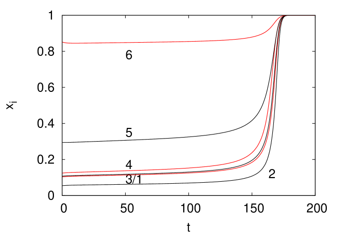
Figure 10: Time evolution for the initial condition $(0.1036,5.477~{}10^{-2},0.107,0.124,0.294,0.851)$ for $\epsilon=1.3~{}10^{-1}$ close to the critical value $\epsilon_{0}=1.25~{}10^{-1}$ for the Zeldovich equation. The parameter $a=0.3$.

The time evolution of the initial condition (69) is presented in Fig. 10. Note the large velocity with which the front ”invades” the network. For $a=0.1$, in Fig. 3 we had a well separated dynamics of node 5 which destabilized first. Here we cannot distinguish the evolution of node 5 from the one of the other nodes. Since the front is much wider, it averages out the network and propagates much faster.

Because the front becomes very wide, the formula (23) will underestimate the critical $\epsilon$. Table 2 shows $\epsilon_{0}$ for $a=0.1,~{}0.2$ and $0.3$ obtained for the static solution centered on node 6.

$a$	$\epsilon_{0}$	expression (23)
0.1	$3.~{}10^{-3}$	$2.8~{}10^{-3}$
0.2	$1.6~{}10^{-2}$	$1.28~{}10^{-2}$
0.3	$1.25~{}10^{-1}$	$3.48~{}10^{-2}$

Table 2: Critical $\epsilon$ for the ”generalized front” centered on node 6 to destabilize for different values of $a$.

As expected (23) underestimates $\epsilon_{0}$ as $a$ increases. It gives the right order of magnitude for $a=0.2$ but is clearly wrong for $a=0.3$.

6 Conclusion

We studied analytically and numerically a bistable reaction diffusion on an arbitrary finite network. We show that stable static fronts exist everywhere on the network for small diffusivity. We give the asymptotics of these fixed points and derive from them a simple depinning criterion which is validated both by continuation techniques and by solving the time dependent problem. The justification of the depinning criterion is an open problem, and may be related to the small value of the local excitation parameter $a$. The numerical simulations suggest that the moving front ”feels” the different static configurations, as it travels accross the network.

We also compare different solutions of the Zeldovich model and show how ”large” fronts dominate ”small” fronts in the dynamics. The time dependent solutions of the Fisher and Kermack-Mckendrick original models are compared to the ones of the Zeldovich; they have a much shorter time scale and no treshold. This effect might be expected from the instability of the origin in the Fisher and Kermack-Mckendrick models. This seems to reduce their interest as opposed to the Zeldovich model. On the other hand all three models describe qualitatively similar front expansion scenarios above the Zeldovich threshold. Another posibility is that The behavior of the Zeldovich model below the highest branch threshold may reflect some pinning phenomena related to epidemics.

Finally we investigate numerically larger local excitation thresholds and show that fronts become wider and travel much faster across the network.

Acknowledgements
J.G. C. thanks the Universidad Nacional Autónoma de México for its hospitality during two visits. The work of J.G. C. is supported partially by a grant from the Grand Reseau de Recherche, Transport Logistique et Information of the Haute-Normandie region. The authors acknowledge the Centre de Ressources Informatiques de Haute Normandie for the computations together with Ana Perez and Ramiro Chavez from IIMAS UNAM for technical support.

References

- [1] A. C. Scott “Nonlinear science, emergence and dynamics of coherent structures”, Oxford University Press (2003).
- [2] F. R. N. Nabarro, ”Dislocations in a simple cubic lattice”, Proc. Roy. Soc. London, 59, 256-272, (1947).
-
[3]
J.-G. Caputo, A. Knippel and E. Simo, ”Oscillations of simple networks”,
J. Phys. A: Math. Theor. 46, 035100 (2013)
http://arxiv.org/abs/1109.3071 - [4] A. Carpio and L. Bonilla , ”Depinning transitions in discrete reaction-diffusion equations”, SIAM J. Appl. Math. 63, 1056-1082, (2003).
- [5] G. Cruz-Pacheco, L. Duran, L. Esteva, A.A. Minzoni, M.Lopez-Cervantes, P. Panayotaros, A. Ahued-Ortega, I. Villaseñor Ruiz, Modelling of the influenza A(H1N1) outbreak in Mexico City, April-May 2009, with control measures, Eurosurveillance 14, 26 (2009)
- [6] M. Gondran and M. Minoux, ”Graphs and Algorithms”, John Wiley and Sons, (1984).
- [7] T. Erneux, G. Nicolis, Propagating fronts in discrete bistable reaction-diffusion system, Physica D 67, 237-244 (1993)
- [8] A. Hoffman and J. Mallet-Paret, ”Universality of Crystallographic Pinning”, J. Dyn. Diff. Equat. 22, 79-119, (2010).
- [9] D. Cvetkovic, P. Rowlinson and S. Simic, ”An Introduction to the Theory of Graph Spectra”, London Mathematical Society Student Texts (No. 75), (2001).
- [10] W. O. Kermack and A. G. McKendrick, “A Contribution to the Mathematical Theory of Epidemics”, Proc. Roy. Soc. Lond. A 115, 700-721 (1927).
- [11] E. Hairer, S. P. Norsett and G. Wanner. Solving ordinary differential equations I, Springer-Verlag, (1987).
- [12] A. Iserles, First Course in the Numerical Analysis of Differential Equations, 2nd Edition, Cambridge University Press Cambridge (2008)
- [13] J.P. Keener, Propagation and its failure in coupled systems of discrete excitable cells, SIAM J. of Appl. Math. 47, 556-572 (1987)
- [14] H.B. Keller, Numerical solution of bifurcation and nonlinear eigenvalue problems, in P. H. Rabinowitz, editor, Applications of Bifurcation Theory, Academic Press (1977)
- [15] R.S. MacKay, S. Aubry: Proof of existence of breathers for time-reversible or Hamiltonian networks of weakly coupled oscillators, Nonlinearity 7, 1623-1643 (1994)
- [16] M.J.D. Powell, A hybrid method for nonlinear equations, in Numerical methods for nonlinear algebraic equations, P. Rabinowitz, ed., Gordon and Breach, New York (1970)
- [17] E. Zeidler, Nonlinear Funcional Analysis and its Applications I, Springer, New York (1986)
-
[18]
The Mathworks
http://www.mathworks.com